A lattice computation of the leading-order hadronic contribution to the muon anomalous magnetic moment can potentially help reduce the error on the Standard Model prediction for this quantity, if sufficient control of all systematic errors affecting such a computation can be achieved. One of these systematic errors is that associated with the extrapolation to the physical pion mass from values on the lattice larger than the physical pion mass. We investigate this extrapolation assuming lattice pion masses in the range of 200 to 400 MeV with the help of two-loop chiral perturbation theory, and find that such an extrapolation is unlikely to lead to control of this systematic error at the 1% level. This remains true even if various tricks to improve the reliability of the chiral extrapolation employed in the literature are taken into account. In addition, while chiral perturbation theory also predicts the dependence on the pion mass of the leading-order hadronic contribution to the muon anomalous magnetic moment as the chiral limit is approached, this prediction turns out to be of no practical use, because the physical pion mass is larger than the muon mass that sets the scale for the onset of this behavior.

I Introduction

Recently, there has been an increasing interest in a high-precision lattice computation of the leading-order hadronic vacuum polarization (HVP) contribution to the muon anomalous magnetic moment, $a_{\mu}^{\rm HLO}$. We refer to Ref. Wittiglat16 for a recent review, and to Refs. AB2007 ; Fengetal ; UKQCD ; DJJW2012 ; FHHJPR ; HPQCDstrange ; BE ; HPQCDdisconn ; RBCdisconn ; HPQCD ; RBCstrange ; BMW16 for efforts in this direction. The aim is to use the methods of lattice QCD to arrive at a value for $a_{\mu}^{\rm HLO}$ with a total error of one-half to one percent or less. Such a result would help solidify, and eventually reduce, the total error on the Standard-Model value of the total muon anomalous magnetic moment $a_{\mu}$, which is currently dominated by the error on the HVP contribution. This desired accuracy requires both a high-statistics computation of the HVP, in particular at low momenta (or, equivalently, at large distance), as well as a theoretically clean understanding of the behavior of the HVP as a function of the Euclidean squared-momentum $Q^{2}$ Pade ; taumodel ; strategy , in order to help in reducing systematic errors. In addition, it is important to gain a thorough understanding of various other systematic errors afflicting the computation, such as those caused by a finite volume BM ; Mainz ; ABGPFV ; Lehnerlat16 , scale setting uncertainties, and the use of lattice ensembles with light quark masses larger than their physical values. Isospin breaking, electromagnetic effects, the presence of dynamical charm and the contribution of quark-disconnected diagrams also all enter at the percent level, and thus also have to be understood quantitatively with sufficient precision.

In this article, we consider the extrapolation of $a_{\mu}^{\rm HLO}$ from heavier than physical pion masses to the physical point, with the help of chiral perturbation theory (ChPT). While lattice computations are now being carried out on ensembles with light quark masses chosen such that the pion mass is approximately physical, a number of computations obtain the physical result via extrapolation from heavier pion masses, while others incorporate results from heavier pion masses in the fits used to convert near-physical-point to actual-physical-point results. The use of such heavier-mass ensembles has a potential advantage since increasing pion mass typically corresponds to decreasing statistical errors on the corresponding lattice data. It is thus important to investigate the reliability of extrapolations of $a_{\mu}^{\rm HLO}$ from such heavier masses, say, $m_{\pi}\approx 200$ MeV or above, to the physical pion mass.

The leading hadronic contribution is given in terms of the hadronic vacuum polarization, and can be written as ER ; TB2003

$$a_{\mu}^{\rm HLO} = -4\alpha^{2}\int_{0}^{\infty}\frac{dQ^{2}}{Q^{2}}\,w(Q^{2})\,\Pi_{\rm sub}(Q^{2})\ ,$$ (1a)

$$w(Q^{2}) = \frac{m_{\mu}^{2}Q^{4}Z^{3}(Q^{2})(1-Q^{2}Z(Q^{2}))}{1+m_{\mu}^{2}Q^{2}Z^{2}(Q^{2})}\ ,$$ (1b)

$$Z(Q^{2}) = \frac{\sqrt{Q^{4}+4m_{\mu}^{2}Q^{2}}-Q^{2}}{2m_{\mu}^{2}Q^{2}}\ ,$$ (1c)

$$\Pi_{\rm sub}(Q^{2}) = \Pi(Q^{2})-\Pi(0)\ ,$$ (1d)

where $\Pi(Q^{2})$, defined by

$$\Pi_{\mu\nu}(Q)=(Q^{2}\delta_{\mu\nu}-Q_{\mu}Q_{\nu})\Pi(Q^{2})\ ,$$ (2)

is the vacuum polarization of the electromagnetic (EM) current, $\alpha$ is the fine-structure constant, and $m_{\mu}$ is the muon mass.

If we wish to use ChPT, we are restricted to considering only the low-$Q^{2}$ part of this integral, because the ChPT representation of $\Pi_{\rm sub}(Q^{2})$ is only valid at sufficiently low values of $Q^{2}$ (as will be discussed in more detail in Sec. III.2). In view of this fact, we will define a truncated $a_{\mu}^{\rm HLO}(Q^{2}_{max})$:

$$a_{\mu}^{\rm HLO}(Q^{2}_{max})=-4\alpha^{2}\int_{0}^{Q^{2}_{max}}\frac{dQ^{2}}{Q^{2}}\,w(Q^{2})\,\Pi_{\rm sub}(Q^{2})\ ,$$ (3)

and work with $Q^{2}_{max}$ small enough to allow for the use of ChPT.

In order to check over which $Q^{2}$ range we can use ChPT, we need data to compare with. Here, we will compare to the subtracted vacuum polarization obtained using the non-strange $I=1$ hadronic vector spectral function measured in $\tau$ decays by the ALEPH collaboration ALEPH13 . Of course, in addition to the $I=1$ part $\Pi^{33}(Q^{2})$, the vacuum polarization also contains an $I=0$ component $\Pi^{88}(Q^{2})$ (and, away from the isospin limit, a mixed isovector-isoscalar component as well). In the isospin limit,

$$\Pi_{\rm EM}(Q^{2})={1\over 2}\,\Pi^{{33}}(Q^{2})+\frac{1}{6}\,\Pi^{{88}}(Q^{2})\ ,$$ (4)

where $\Pi^{33}$ and $\Pi^{88}$ are defined from the octet vector currents

$$V_{\mu}^{3} = \frac{1}{\sqrt{2}}\left(V_{\mu}^{uu}-V_{\mu}^{dd}\right)\ ,$$ (5)

$$V_{\mu}^{8} = \frac{1}{\sqrt{6}}\left(V_{\mu}^{uu}+V_{\mu}^{dd}-2V_{\mu}^{ss}\right)\ ,$$

with the EM current given by

$$V^{\rm EM}_{\mu}=\frac{1}{\sqrt{2}}\left(V^{3}_{\mu}+\frac{1}{\sqrt{3}}\,V^{8}_{\mu}\right)\ .$$ (6)

Here $V_{\mu}^{uu}=\overline{u}\gamma_{\mu}u$, $V_{\mu}^{dd}=\overline{d}\gamma_{\mu}d$ and $V_{\mu}^{ss}=\overline{s}\gamma_{\mu}s$. The quantity we will thus primarily consider in this article is

$$\tilde{a}_{\mu}(Q^{2}_{max})=-4\alpha^{2}\int_{0}^{Q^{2}_{max}}\frac{dQ^{2}}{Q^{2}}\,w(Q^{2})\,\Pi^{{33}}_{\rm sub}(Q^{2})\ ,$$ (7)

where we will choose $Q^{2}_{max}=0.1$ GeV² (cf. Sec. III.2 below). In Sec. IV.3 we will consider also the inclusion of the $I=0$ contribution.

It is worth elaborating on why we believe the quantity $\tilde{a}_{\mu}(Q^{2}_{max}=0.1~{}\mbox{GeV}^{2})$ will be useful for studying the extrapolation to the physical pion mass, in spite of the fact that it constitutes only part of $a_{\mu}^{\rm HLO}$. First, the $I=1$ threshold is $s=4m_{\pi}^{2}$, while that for $I=0$ is $s=9m_{\pi}^{2}$. This suggests that the $I=1$ part of $a_{\mu}^{\rm HLO}$ should dominate the chiral behavior. Second, from the dispersive representation, it is clear that the relative contributions to $\Pi_{\rm sub}(Q^{2})$ from the region near the two-pion threshold are larger at low $Q^{2}$ than they are at high $Q^{2}$. Contributions to $a_{\mu}^{\rm HLO}$ from the low-$Q^{2}$ part of the integral in Eq. (1a) are thus expected to be relatively more sensitive to variations in the pion mass than are those from the rest of the integral. The part of the integral below $Q^{2}_{max}=0.1$ GeV², moreover, yields about 80% of $a_{\mu}^{\rm HLO}$. We thus expect a study of the chiral behavior of $\tilde{a}_{\mu}(Q^{2}_{max}=0.1~{}\mbox{GeV}^{2})$ to provide important insights into the extrapolation to the physical pion mass. This leaves out the contribution from the integral above $0.1$ GeV², which can be accurately computed directly from the lattice data using a simple trapezoidal rule evaluation taumodel ; strategy . Its pion mass dependence is thus not only expected to be milder, for the reasons given above, but also to be amenable to a direct study using lattice data. In light of these comments, it seems to us highly unlikely that adding the significantly smaller ($\sim 20\%$) $Q^{2}>0.1$ GeV² contributions, with their weaker pion mass dependence, could produce a complete integral with a significantly reduced sensitivity to the pion mass.

This paper is organized as follows. In Sec. II we collect the needed expressions for the HVP to next-to-next-to-leading order (NNLO) in ChPT, and derive a formula for the dependence of $a_{\mu}^{\rm HLO}$ on the pion mass in the limit $m_{\pi}\to 0$. In Sec. III we compare the $I=1$ ChPT expression with the physical $\Pi^{{33}}_{\rm sub}(Q^{2})$, constructed from the ALEPH data, and argue that $\tilde{a}_{\mu}(Q^{2}_{max}=0.1~{}\mbox{GeV}^{2})$ can be reproduced to an accuracy of about 1% in ChPT. Section IV contains the study of the extrapolation of $\tilde{a}_{\mu}(Q^{2}_{max}=0.1~{}\mbox{GeV}^{2})$ computed at pion masses typical for the lattice, also considering various tricks that have been considered in the literature to modify $a_{\mu}^{\rm HLO}$ at larger pion mass in such a way as to weaken the pion-mass-dependence of the result and thus improve the reliability of the thus-modified chiral extrapolation. We end this section with a discussion of the inclusion of the $I=0$ part. We present our conclusions in Sec. V, and relegate some technical details to an appendix.

II The vacuum polarization in chiral perturbation theory

In this section we collect the NNLO expressions for $\Pi^{{33}}(Q^{2})$ and $\Pi^{{88}}(Q^{2})$ as a function of Euclidean $Q^{2}$, summarizing the results of Refs. GK95 ; ABT . Using the conventions of Ref. ABT , one has

$$\Pi^{{33}}_{\rm sub}(Q^{2}) = -8\hat{B}(Q^{2},m_{\pi}^{2})-4\hat{B}(Q^{2},m_{K}^{2})$$

$$+\frac{16}{f_{\pi}^{2}}\,L_{9}^{r}\,Q^{2}\left(2B(Q^{2},m_{\pi}^{2})+B(Q^{2},m_{K}^{2})\right)$$

$$-\frac{4}{f_{\pi}^{2}}\,Q^{2}\left(2B(Q^{2},m_{\pi}^{2})+B(Q^{2},m_{K}^{2})\right)^{2}$$

$$+8C_{93}^{r}Q^{2}+C^{r}(Q^{2})^{2}\ ,$$

and

$$\Pi^{{88}}_{\rm sub}(Q^{2}) = -12\hat{B}(Q^{2},m_{K}^{2})$$

$$+\frac{48}{f_{\pi}^{2}}\,L_{9}^{r}\,Q^{2}B(Q^{2},m_{K}^{2})-\frac{36}{f_{\pi}^{2}}\,Q^{2}\left(B(Q^{2},m_{K}^{2})\right)^{2}$$

$$+8C_{93}^{r}Q^{2}+C^{r}(Q^{2})^{2}\ ,$$

where $B(Q^{2},m^{2})=B(0,m^{2})+\hat{B}(Q^{2},m^{2})$ is the subtracted standard equal-mass, two-propagator, one-loop integral, with

$$B(0,m^{2}) = \frac{1}{192\pi^{2}}\left(1+\log{\frac{m^{2}}{\mu^{2}}}\right)\ ,$$ (10)

$$\hat{B}(Q^{2},m^{2}) = \frac{1}{96\pi^{2}}\left(\left(\frac{4m^{2}}{Q^{2}}+1\right)^{3/2}\mbox{coth}^{-1}\sqrt{1+\frac{4m^{2}}{Q^{2}}}-\frac{4m^{2}}{Q^{2}}-{\frac{4}{3}}\right)\ ,$$

and the low-energy constants (LECs) $L_{9}^{r}$ and $C_{93}^{r}$ are renormalized at the scale $\mu$, in the “$\overline{MS}+1$” scheme employed in Ref. ABT . Note that these are the only two LECs appearing in the subtracted versions of the $I=1$ and $I=0$ non-strange vacuum polarizations to NNLO.

As in Ref. strategy , we have added an analytic NNNLO term, $C^{r}(Q^{2})^{2}$, to $\Pi^{33}_{\rm sub}(Q^{2})$ and $\Pi^{88}_{\rm sub}(Q^{2})$ in order to improve, in the $I=1$ case, the agreement with $\Pi^{{33}}_{\rm sub}(Q^{2})$ constructed from the ALEPH data, as we will see in Sec. III below. Such a contribution, which would first appear at NNNLO in the chiral expansion, and be produced by six-derivative terms in the NNNLO Lagrangian, will necessarily appear with the same coefficient in both the $I=0$ and $I=1$ polarizations at NNNLO. Following Ref. strategy , we will refer to the expressions with $C^{r}=0$ as “NNLO,” and with the $C^{r}$ term included as “NN^′LO.”

From these expressions, it is clear that the chiral behavior of $a_{\mu}^{\rm HLO}$, which we expect to be primarily governed by the pion, rather than kaon, contributions, will be dominated by the $I=1$ component. In fact, in the limit that $m_{\pi}\to 0$ with $m_{\mu}$ fixed, we find

$$a_{\mu}^{I=1} \equiv \tilde{a}_{\mu}(Q^{2}_{max}=\infty)=$$

$$\frac{\alpha^{2}}{12\pi^{2}}\left(-\log{\frac{m_{\pi}^{2}}{m_{\mu}^{2}}}-\frac{31}{6}+3\pi^{2}\sqrt{\frac{m_{\pi}^{2}}{m_{\mu}^{2}}}+O\left(\frac{m_{\pi}^{2}}{m_{\mu}^{2}}\log^{2}{\frac{m_{\pi}^{2}}{m_{\mu}^{2}}}\right)\right)\ .$$

A derivation of this result is given in App. A. We note that the scale for the chiral extrapolation is set by the muon mass, and thus Eq. (II) applies to the region $m_{\pi}\ll m_{\mu}$. Therefore, this result is unlikely to be of much practical value. Indeed, our tests in Sec. IV below will confirm this expectation.

III Comparison with ALEPH data for hadronic $\tau$ decays

In this section, we will construct $\Pi^{{33}}_{\rm sub}(Q^{2})$ from the non-strange, vector spectral function $\rho^{{33}}_{V}$ measured by ALEPH in hadronic $\tau$ decays ALEPH13 , using the once-subtracted dispersion relation

$$\Pi^{{33}}_{\rm sub}(Q^{2})=-Q^{2}\int_{4m_{\pi}^{2}}^{\infty}ds\,\frac{\rho^{{33}}_{V}(s)}{s(s+Q^{2})}\ .$$ (12)

Since the spectral function is only measured for $s\leq m_{\tau}^{2}$, this is not entirely trivial, and we will describe our construction in more detail in Sec. III.1. We then compare the data with ChPT in Sec. III.2.

III.1 $\Pi^{{33}}_{\rm sub}(Q^{2})$ from ALEPH data

In order to construct $\rho^{{33}}_{V}(s)$ for $s>m_{\tau}^{2}$, we follow the same procedure as in the $V-A$ case considered in Refs. L10 ; VmAALEPH . For a given $s_{min}\leq m_{\tau}^{2}$, we switch from the data representation of $\rho^{{33}}_{V}(s)$ to a theoretical representation given by the sum of the QCD perturbation theory (PT) expression $\rho^{{33}}_{V,{\rm PT}}(s)$ and a “duality-violating” (DV) part $\rho^{{33}}_{V,{\rm DV}}(s)$ that represents the oscillations around perturbation theory from resonances, and which we model as

$$\rho^{{33}}_{V,{\rm DV}}(s)=e^{-\delta_{V}-\gamma_{V}s}\sin{(\alpha_{V}+\beta_{V}s)}\ .$$ (13)

The perturbative expression is known to order $\alpha_{s}^{4}$ PT , where $\alpha_{s}=\alpha_{s}(m_{\tau}^{2})$ is the strong coupling. Fits to the ALEPH data determining the parameters $\alpha_{s}$, $\alpha_{V}$, $\beta_{V}$, $\gamma_{V}$ and $\delta_{V}$ have been extensively studied in Ref. alphas14 , with the goal of a high-precision determination of $\alpha_{s}$ from hadronic $\tau$ decays. Here we will use the values obtained from the FOPT $s_{min}=1.55$ GeV² fit of Table 1 of Ref. alphas14 ,

$$\alpha_{s}(m_{\tau}^{2}) = 0.295(10)\ ,$$ (14)

$$\alpha_{V} = -2.43(94)\ ,$$

$$\beta_{V} = 4.32(48)\ \mbox{GeV}^{-2}\ ,$$

$$\gamma_{V} = 0.62(29)\ \mbox{GeV}^{-2}\ ,$$

$$\delta_{V} = 3.50(50)\ .$$

The match between the data and theory representations of the spectral function in the window $s_{min}\leq s\leq m_{\tau}^{2}$ is excellent, and there is no discernible effect on $\Pi^{{33}}_{\rm sub}(Q^{2})$ for the values of $Q^{2}$ smaller than $0.2$ GeV² of interest in the comparison to ChPT below if we use a different switch point from data to theory inside this interval, switch to a CIPT instead an FOPT fit, or if we use the parameter values of one of the other optimal fits in Ref. alphas14 . Results for $\Pi^{{33}}_{\rm sub}(Q^{2})$ in the region below $Q^{2}=0.2$ GeV², at intervals of $0.01$ GeV², are shown in Fig. 1. The errors shown are fully correlated, taking into account, in particular, correlations between the parameters of Eq. (14) and the data.

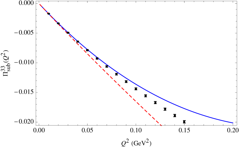
Figure 1: $\Pi^{{33}}_{\rm sub}(Q^{2})$ as a function of $Q^{2}$. Black points: data, constructed as explained in Sec. III.1; red (lower) curve: NNLO ChPT representation with $C^{r}=0$; blue (upper) curve: NN^′LO ChPT representation with $C^{r}$ as determined from the data. For the ChPT representations, see Sec. III.2.

III.2 Comparison with ChPT

In order to compare the data for $\Pi^{{33}}_{\rm sub}(Q^{2})$ with ChPT, we need values for $L_{9}^{r}$, $C^{r}_{93}$ and $C^{r}$. Although, in principle, they can all be obtained from a fit to the ALEPH data, in practice $L_{9}^{r}$ and $C^{r}_{93}$ turn out to be strongly anti-correlated, making it difficult to determine these two LECs separately from these data. We thus, instead, use an external value for $L_{9}^{r}$ taken from the NNLO analysis of Ref. BTL9 :

$$L^{r}_{9}(\mu=0.77~{}\mbox{GeV})=0.00593(43)\ .$$ (15)

With this value, a fit to the slope and curvature at $Q^{2}=0$ of $\Pi^{{33}}_{\rm sub}(Q^{2})$ is straightforward, and we find

$$C^{r}_{93}(\mu=0.77~{}\mbox{GeV}) = -0.0154(4)\ \mbox{GeV}^{-2}\ ,$$ (16)

$$C^{r}(\mu=0.77~{}\mbox{GeV}) = 0.29(3)\ \mbox{GeV}^{-4}\ .$$

The determination of $C^{r}_{93}$ is new, and will be discussed in more detail in a forthcoming publication C93 . Here, we will use the central values in a comparison between the data and ChPT, in order to see with what accuracy $\tilde{a}_{\mu}(Q^{2}_{max})$ can be represented in ChPT, as a function of $Q^{2}_{max}$.

The two curves in Fig. 1 show ChPT representations of $\Pi^{{33}}_{\rm sub}(Q^{2})$. The blue solid curve corresponds to NN^′LO ChPT, employing the values (15) and (16), the red dashed curve to NNLO ChPT, obtained by dropping the $C^{r}(Q^{2})^{2}$ contribution from the fitted NN^′LO result. It is clear that allowing for the analytic NNNLO term in ChPT helps improve the agreement with the data, even though this falls short of a full NNNLO comparison.

We may now compare values of $\tilde{a}_{\mu}(Q^{2}_{max})$ computed from the data and from ChPT, as a function of $Q^{2}_{max}$. For $Q^{2}_{max}=0.1$ GeV² we find

$$\tilde{a}_{\mu}(0.1\ \mbox{GeV}^{2})=\left\{\begin{array}[]{ll}9.81\times 10^{-8}&\qquad\mbox{data\ ,}\\ 9.73\times 10^{-8}&\qquad\mbox{NN${}^{\prime}$LO ChPT}\ ,\\ 10.23\times 10^{-8}&\qquad\mbox{NNLO ChPT}\ .\end{array}\right.$$ (17)

We do not show errors, because we are only interested in the ChPT values for $\tilde{a}_{\mu}(Q^{2}_{max})$ as a model to study the pion mass dependence. However, Eq. (17) shows that NN^′LO ChPT reproduces the data value for $\tilde{a}_{\mu}(0.1\ \mbox{GeV}^{2})$ to about 1%, and that the addition of the $C^{r}$ term to Eq. (II) improves this agreement from about 4%. With the value of $\tilde{a}_{\mu}=\tilde{a}_{\mu}(\infty)=11.95\times 10^{-8}$ computed from the data we also see that the $Q^{2}_{\max}=0.1$ GeV² value amounts to 82% of the full integral. For $Q^{2}_{max}=0.2$ GeV² we find, similarly,

$$\tilde{a}_{\mu}(0.2\ \mbox{GeV}^{2})=\left\{\begin{array}[]{ll}10.96\times 10^{-8}&\qquad\mbox{data\ ,}\\ 10.77\times 10^{-8}&\qquad\mbox{NN${}^{\prime}$LO ChPT}\ ,\\ 11.61\times 10^{-8}&\qquad\mbox{NNLO ChPT}\ .\end{array}\right.$$ (18)

For $Q^{2}_{\max}=0.2$ GeV² the presence of $C^{r}$ improves the agreement between the ChPT and data values from about 6% to about 2%, and the truncated integral provides 92% of the full result.

It is remarkable that ChPT does such a good job for $\tilde{a}_{\mu}(Q^{2}_{max})$ for these values of $Q^{2}_{max}$, and that such low values of $Q^{2}_{max}$ already represent such a large fraction of the integral (7) for $Q^{2}_{max}=\infty$. The reason is that the integrand of Eq. (7) is strongly peaked at $Q^{2}\approx m_{\mu}^{2}/4=0.0028$ GeV². Below, we will use values of $\tilde{a}_{\mu}(Q^{2}_{max})$ computed with $Q^{2}_{\max}=0.1$ GeV² for our study of the pion mass dependence.

IV Chiral extrapolation of $\tilde{a}_{\mu}(Q^{2}_{max})$

The pion mass dependence of $\tilde{a}_{\mu}(Q^{2}_{max})$, as it would be computed on the lattice, has a number of different sources. Restricting ourselves to $Q^{2}_{max}=0.1$ GeV², we can use ChPT to trace these sources. In addition to the explicit dependence on $m_{\pi}$ in Eq. (II), $m_{K}$ and $f_{\pi}$ also depend on the pion mass. Although $C_{93}^{r}$ and $C^{r}$ represent LECs of the effective chiral Lagrangian and hence are mass-independent, the data includes contributions of all chiral orders. Thus, when we perform fits using the truncated NNLO and NN^′LO forms, the resulting LEC values, in general, will become effective ones, in principle incorporating mass-dependent contributions from terms higher order in ChPT than those shown in Eq. (II). These will, in general, differ from the true mass-independent LECs $C_{93}^{r}$ and $C^{r}$ due to residual higher-order mass-dependent effects. These same effects would also cause the values obtained from analogous fits to lattice data for ensembles with unphysical pion mass to differ from the true, mass-independent values. We will denote the general mass-dependent effective results by $C_{93,{\rm eff}}^{r}$ and $C^{r}_{\rm eff}$, and model their mass dependence by assuming the fitted values in Eq. (16) are dominated by the contributions of the $\rho$ resonance strategy ; ABT . With this assumption,

$$C_{93,{\rm eff}}(\mu=0.77~{}\mbox{GeV}) = -\frac{f_{\rho}^{2}}{4m_{\rho}^{2}}\ ,$$ (19)

$$C^{r}_{\rm eff}(\mu=0.77~{}\mbox{GeV}) = \frac{2f_{\rho}^{2}}{m_{\rho}^{4}}\ ,$$

with $m_{\rho}$ and $f_{\rho}$ in general dependent on the pion mass. We will suppress the explicit $m_{\pi}$ dependence of $C_{93,{\rm eff}}^{r}$ and $C^{r}_{\rm eff}$ except where a danger of confusion exists. For physical light quark mass, with $f_{\rho}\approx 0.2$ and $m_{\rho}=0.775$ GeV, we find $C_{93,{\rm eff}}(m_{\pi}^{2})\approx-0.017$ GeV^-2, and $C^{r}_{\rm eff}(m_{\pi}^{2})\approx 0.22$ GeV^-4. These values are in quite reasonable agreement with Eq. (16).

On the lattice, one finds that $m_{\rho}$ is considerably more sensitive to the pion mass than is $f_{\rho}$ Fengetal . We thus model the pion mass dependence of $C^{r}_{93,{\rm eff}}$ and $C^{r}_{\rm eff}$ by assuming the effective $\mu=0.77$ GeV values are given by

$$C^{r}_{93,{\rm eff}}(m_{\pi,latt}^{2}) = C^{r}_{93,{\rm eff}}(m_{\pi}^{2})\,\frac{m_{\rho}^{2}}{m_{\rho,{\rm latt}}^{2}}\ ,$$ (20)

$$C^{r}_{\rm eff}(m_{\pi,latt}^{2}) = C^{r}_{{\rm eff}}(m_{\pi}^{2})\,\frac{m_{\rho}^{4}}{m_{\rho,{\rm latt}}^{4}}\ .$$

where $m_{\rho,{\rm latt}}$ is the $\rho$ mass computed on the lattice.

This strategy allows us to generate a number of fake lattice data for $\tilde{a}_{\mu}(Q^{2}_{max})$ using ChPT. For each $m_{\pi}$ in the range of interest, the corresponding $m_{\rho}$ is needed to compute $C_{93,{\rm eff}}^{r}$ and $C_{\rm eff}^{r}$ via Eqs. (20). This information is available, over the range of $m_{\pi}$ we wish to study, for the HISQ ensembles of the MILC collaboration MILC , and we thus use the following set of values for $m_{\pi}$, $f_{\pi}$, $m_{K}$ and $m_{\rho}$, corresponding to those ensembles:

$$\begin{array}[]{|c|c|c|c|}\hline\cr m_{\pi}\ (\mbox{MeV})&f_{\pi}\ (\mbox{MeV})&m_{K}\ (\mbox{MeV})&m_{\rho}\ (\mbox{MeV})\\ \hline\cr 223&98&514&826\\ 262&101&523&836\\ 313&104&537&859^{*}\\ 382&109&558&894\\ 440&114&581&929\\ \hline\cr\end{array}\vspace{2ex}$$ (21)

The statistical errors on these numbers are always smaller than 1%, except for the $\rho$ mass marked with an asterisk. In fact, the (unpublished) MILC value for this $\rho$ mass is $834(30)$ MeV. Since we are interested in constructing a model, we corrected this value by linear interpolation in $m_{\pi}^{2}$ between the two neighboring values, obtaining the value $859$ MeV, which is consistent within errors with the MILC value. With this correction, $f_{\pi}$, $m_{K}$ and $m_{\rho}$ are all approximately linear in $m_{\pi}^{2}$.

IV.1 The ETMC trick

Before starting the numerical study of our ChPT-based model, we outline a trick aimed at modifying $a_{\mu}^{\rm HLO}$ results at heavier pion masses in such a way as to weaken the resulting pion mass dependence, and thus improve the reliability of the extrapolation to the physical pion mass. The trick, first introduced in Ref. Fengetal , is best explained using an example. Consider the following very simple vector-meson dominance (VMD) model for $\Pi^{{33}}(Q^{2})$ MHA :

$$\Pi^{{33}}_{\rm VMD,sub}(Q^{2})=-\frac{2f_{\rho}^{2}Q^{2}}{Q^{2}+m_{\rho}^{2}}-\frac{1}{4\pi^{2}}\log{\left(1+\frac{Q^{2}}{8\pi^{2}f_{\rho}^{2}m_{\rho}^{2}}\right)}\ .$$ (22)

The logarithm is chosen such that it reproduces the parton-model logarithm while at the same time generating no $1/Q^{2}$ term for large $Q^{2}$. The (simplest version of the) ETMC trick consists of inserting a correction factor $m_{\rho,{\rm latt}}^{2}/m_{\rho}^{2}$ in front of $Q^{2}$ in the subtracted HVP before carrying out the integral over $Q^{2}$ in Eq. (1). If we assume that $f_{\rho}$ does not depend on $m_{\pi}$ but $m_{\rho}$ does, it is easily seen that the resulting ETMC-modified version of $\Pi^{{33}}_{\rm VMD,sub}(Q^{2})$, $\Pi^{{33}}_{\rm VMD,sub}\left({\frac{m_{\rho,{\rm latt}}^{2}}{m_{\rho}^{2}}}Q^{2}\right)$, is completely independent of $m_{\pi}$. With the VMD form known to provide a reasonable first approximation to $\Pi^{{33}}_{\rm sub}(Q^{2})$, the application of the ETMC trick to actual lattice results is thus expected to produce a modified version of $a_{\mu}^{\rm HLO}$ displaying considerably reduced $m_{\pi}$ dependence. In Ref. Fengetal a further change of variable was performed to shift the modification factor out of the argument of the HVP and into that of the weight function, the result being a replacement of the argument $Q^{2}$ in $w(Q^{2})$ by $\left(m_{\rho}^{2}/m_{\rho,{\rm latt}}^{2}\right)Q^{2}$. We do not perform this last change of variable since, in our study, we cut off the integral at $Q^{2}=Q^{2}_{max}$, cf. Eqs. (3) and (7).

In Ref. HPQCD a variant of this trick was used as follows. First, the HVP was modified to remove what was expected to be the strongest pion mass dependence by subtracting from the lattice version of $\Pi^{{33}}_{\rm sub}(Q^{2})$ the NLO pion loop contribution (effectively, from our perspective, the first term of Eq. (II)), evaluated at the lattice pion mass, $m_{\pi,{\rm latt}}$. The ETMC rescaling, $Q^{2}\to(m_{\rho,{\rm latt}}^{2}/m_{\rho}^{2})Q^{2}$, was then applied to the resulting differences and the extrapolation to physical pion mass performed on these results. Finally, the physical mass version of the NLO pion loop contribution (again, effectively the first term of Eq. (II), now evaluated at physical $m_{\pi}$) was added back to arrive at the final result for $a_{\mu}^{\rm HLO}$. This sequence of procedures is equivalent, in our language, to employing the modified HVP

$$\Pi_{\rm sub,corr}^{33}(Q^{2})=\Pi_{\rm sub}^{33}\left(\frac{m_{\rho,{\rm latt}}^{2}}{m_{\rho}^{2}}\,Q^{2}\right)+8\left(\hat{B}\left(\frac{m_{\rho,{\rm latt}}^{2}}{m_{\rho}^{2}}\,Q^{2},m_{\pi,{\rm latt}}^{2}\right)-\hat{B}(Q^{2},m_{\pi}^{2})\right)\ .$$ (23)

We will refer to this version of the ETMC trick as the HPQCD trick.

IV.2 The $I=1$ case

We have generated three “data” sets based on the results for $\tilde{a}_{\mu}\equiv\tilde{a}_{\mu}(Q^{2}_{max}=0.1$ GeV${}^{2})$, at the five values of $m_{\pi}$ given in Eq. (21), using Eq. (II) with the effective LECs (20). One set consists simply of the five unmodified results for $\tilde{a}_{\mu}$, the other two of the ETMC- and HPQCD-modified version thereof, all obtained using Eq. (II) with the effective LECs (20). We will refer to these three data sets as unimproved, ETMC-improved, and HPQCD-improved in what follows. To avoid a proliferation of notation, and since it should cause no confusion to do so, the ETMC- and HPQCD-modified versions of $\tilde{a}_{\mu}$ will also be denoted by $\tilde{a}_{\mu}$ in what follows.

We performed three fits on each of these three data sets, using the following three functional forms for the dependence on $m_{\pi}$:

$$\tilde{a}_{\mu}^{\rm quad} = Am_{\pi,{\rm latt}}^{4}+Bm_{\pi,{\rm latt}}^{2}+C\hskip 113.81102pt(\mbox{quadratic})\ ,$$ (24a)

$$\tilde{a}_{\mu}^{\rm log} = A\log{(m_{\pi,{\rm latt}}^{2}/m_{\pi}^{2})}+Bm_{\pi,{\rm latt}}^{2}+C\hskip 63.44952pt(\mbox{log})\ ,$$ (24b)

$$\tilde{a}_{\mu}^{\rm inv} = \frac{A}{m_{\pi,{\rm latt}}^{2}}+Bm_{\pi,{\rm latt}}^{2}+C\hskip 119.2171pt(\mbox{inverse})\ .$$ (24c)

The “log” fit is inspired by Eq. (II). The “inverse” fit is essentially that used by HPQCD in Ref. HPQCD . Explicily, without scaling violations, and assuming a physical strange quark mass, the HPQCD fit function takes the form

$$a_{\mu}^{\rm HLO}\left(1+c_{\ell}\,\frac{\delta m_{\ell}}{\Lambda}+{\tilde{c}}_{\ell}\,\frac{\delta m_{\ell}}{m_{\ell}}\right)\ ,$$ (25)

with $\delta m_{\ell}=m_{\ell}-m_{\ell}^{\rm phys}$ and $m_{\ell}$ the average of the up and down quark masses on the lattice. Assuming a linear relation between $m_{\ell}$ and $m_{\pi}^{2}$, this form can be straightforwardly rewritten in the form Eq. (24c).

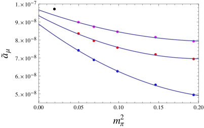
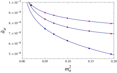
Figure 2: The unmodified and ETMC- and HPQCD-improved versions of $\tilde{a}_{\mu}$ as a function of $m_{\pi}^{2}$. In each plot, the upper (magenta) data points are HPQCD-improved, the middle (red) data points ETMC-improved and the lower (blue) data points unimproved. The (black) point in the upper left corner of each plot is the “physical” point, $\tilde{a}_{\mu}=9.73\times 10^{-8}$ (cf. Eq. (17)). Fits are “quadratic” (upper left panel), “log” (upper right panel) and “inverse” (lower panel). For further explanation, see text.

All three fits on all three data sets are shown in Fig. 2. Clearly, as expected, the ETMC trick, and even more so the HPQCD trick, improve (i.e., reduce) the pion mass dependence of the resulting modified $\tilde{a}_{\mu}$: the values at larger pion masses are closer to the correct “physical” value shown as the black point in the upper left corner of all panels. All fits look good, and the log fits to the ETMC- or HPQCD-improved data approach the correct value. However, the coefficient of the logarithm in Eq. (24b) falls in the range $-1.5\times 10^{-8}$ to $-0.8\times 10^{-8}$, more than an order of magnitude smaller than the value $-4.5\times 10^{-7}$ predicted by Eq. (II). In this respect, we note that the expansion (II) has a chance of being reliable for $m_{\pi}<m_{\mu}$; the log fits, however, are carried out for lattice pion masses which are larger than the physical pion mass, which, in turn, is larger than $m_{\mu}$. We also note that the form (24c) is more singular than predicted by Eq. (II).

We conclude that all three fits are at best phenomenological, with none of the fit forms in Eq. (24) theoretically preferred. We also note that replacing the linear term in $m_{\pi}^{2}$ in Eq. (24b) by a term linear in $m_{\pi}$, as suggested by Eq. (II), does not improve the mismatch between the theoretical and fitted values of the coefficient of the logarithm. All this suggests that the systematic error from the extrapolation to the physical pion mass is hard to control, at least when the lowest lattice pion mass is around $200$ MeV (or, when the statistical error on a value closer to the physical pion mass is too large to sufficiently constrain the extrapolation).

	unimproved data	ETMC-improved data	HPQCD-improved data
quadratic	8.26	8.91	9.38
log	8.96	9.55	9.77
inverse	9.93	10.46	10.33

Table 1: Values for $\tilde{a}_{\mu}\times 10^{8}$ for the three types of fit (cf. Eq. (24)) and the three data sets. For reference, the correct model value is $\tilde{a}_{\mu}\times 10^{8}=9.73$ (cf. Eq. (17)).

In Table 1 we show the values for $\tilde{a}_{\mu}$ at the physical pion mass obtained from the three types of fit to the three data sets. The log-fit value to the HPQCD-improved data is particularly good, missing the correct value by only $0.4\%$. However, as we have seen, the log fit is not theoretically preferred, and without knowledge of the correct value, the only way to obtain an estimate for the systematic error associated with the extrapolation in the real world would be by comparing the results obtained using different fit forms. Discarding the inverse fit as too singular, one may take the (significantly smaller) variation between the quadratic and log fits as a measure of the systematic error. This spread is equal to 8%, 7% and 4%, respectively, for the unimproved, ETMC-improved and HPQCD-improved data sets. Therefore, even though the ETMC and HPQCD tricks do improve the estimated accuracy, they are not sufficiently reliable to reach the desired level of sub-1% accuracy.

We have also carried out the same fits omitting the highest pion mass (of 440 MeV, cf. Eq. (21)), and find this makes very little difference. The extrapolated values reported in Table 1 do not change by more than about $0.5$ to 1%, and there is essentially no change in the systematic uncertainty estimated using the variation with the fit-form choice as we did above.

IV.3 The electromagnetic case

We may repeat the analysis of Sec. IV.2 for the electromagnetic case, i.e., using $\Pi_{\rm EM}(Q^{2})$ instead of $\Pi^{{33}}(Q^{2})$. The only difference is that in this case we do not have a “data” value as in Eqs. (17) and (18), and we have to rely on ChPT alone.

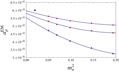
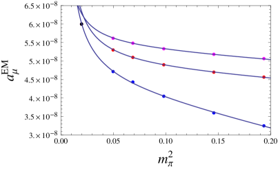
Figure 3: The unmodified and ETMC- and HPQCD-improved versions of $a^{\rm EM}_{\mu}$ as a function of $m_{\pi}^{2}$. In each plot, the upper (magenta) data points are HPQCD-improved, the middle (red) data points ETMC-improved and the lower (blue) data points unimproved. The (black) point in the upper left corner of each plot is the “physical” point, $a^{\rm EM}_{\mu}=6.00\times 10^{-8}$. Fits are “quadratic” (upper left panel), “log” (upper right panel) and “inverse” (lower panel). For further explanation, see text.

Defining the shorthand $a^{\rm EM}_{\mu}=a^{\rm EM}_{\mu}(Q^{2}_{max}=0.1$ GeV${}^{2})$, and using the same notation for the ETMC- and HPQCD-modified versions thereof, we show the quadratic, log and inverse fits for this case in Fig. 3. We see again that the use of the ETMC and HPQCD tricks significantly reduces the pion mass dependence of the resulting modified data, with the HPQCD improvement being especially effective in this regard. The predicted value of the coefficient of the logarithm in the EM analogue of Eq. (II) is now half the value shown in that equation (cf. Eq. (4)), equal to $-2.2\times 10^{-7}$, while the fitted coefficients for the log fits range between $-0.8\times 10^{-8}$ and $-0.4\times 10^{-8}$. The relative difference is of the same order as in the $I=1$ case, and the log fit should thus, as before, be considered purely phenomenological in nature.

	unimproved data	ETMC-improved data	HPQCD-improved data
quadratic	5.19	5.59	5.82
log	5.55	5.91	6.02
inverse	6.04	6.37	6.30

Table 2: Values for $a^{\rm EM}_{\mu}\times 10^{8}$ for the three types of fit (cf. Eq. (24)) and the three data sets. For reference, the correct model value is $a^{\rm EM}_{\mu}\times 10^{8}=6.00$.

In Table 2 we show the values for $a^{\rm EM}_{\mu}$ at the physical pion mass obtained from the three types of fit to the three data sets. The log-fit value to the HPQCD-improved data is particularly good, missing the correct value by only $0.3\%$. Discarding again the inverse fit as too singular, and taking the variation between the quadratic and log fits as a measure of the systematic error, the spread is 6%, 5% and 3%, respectively, for the unimproved, ETMC-improved and HPQCD-improved data sets. Therefore, even though the ETMC and HPQCD tricks do improve the estimated accuracy, this improvement is not sufficient to reach the desired target of sub-1% accuracy. Again, removing the highest pion mass points from the fits makes no signficant difference in these conclusions.

We conclude that, in the electromagnetic case, the situation is slightly better than in the $I=1$ case, no doubt because of the larger relative weight of contributions which are less sensitive to the pion mass (such as the two-kaon contribution). While the ETMC and HPQCD tricks do again improve the estimated accuracy, these improvements remain insufficient to reliably reach the desired sub-1% level.

V Conclusion

In this paper, we used a ChPT-inspired model to investigate the extrapolation of the leading-order hadronic contribution to the muon anomalous magnetic moment, $a_{\mu}^{\rm HLO}$, from lattice pion masses of order 200 to 400 MeV to the physical pion mass. We found that such pion masses are too large to allow for a reliable extrapolation, if the aim is an extrapolation error of less than 1%. This is true even if various tricks to improve the extrapolation are employed, such as those proposed in Ref. Fengetal and Ref. HPQCD .

In order to perform our study, we had to make certain assumptions. First, we assumed that useful insight into the pion mass dependence could be obtained by focussing on the contribution to $a_{\mu}^{\rm HLO}$ from $Q^{2}$ up to $Q^{2}_{max}=0.1$ GeV². This restriction is necessary if we want to take advantage of information on the mass dependence from ChPT, since it is only in this range that ChPT provides a reasonable representation of the HVP. We believe this is not a severe restriction, since that part of the integral yields over 80% of $a_{\mu}^{\rm HLO}$, and it is clear that it is the low-$Q^{2}$ part of the HVP which is most sensitive to the pion mass. Changing $Q^{2}_{max}$ to $0.2$ GeV² makes no qualitative difference to our conclusions.

Second, we assumed Eq. (20) for the dependence of the effective LECs $C^{r}_{93,{\rm eff}}$ and $C^{r}_{\rm eff}$ on the pion mass. While this is a phenomenological assumption, we note that this assumption is in accordance with the ideas underlying the ETMC and HPQCD tricks, so that those tricks should work particularly well if indeed this assumption would be correct in the real world. There are two reasons that the modified extrapolations nevertheless do not work well enough to achieve the desired sub-1% accuracy. One is the fact that in addition to the physics of the $\rho$, the two-pion intermediate state contributing to the non-analytic terms in Eq. (II), not just at one loop, but also beyond one loop, plays a significant role as well. This is especially so because of the structure of the weight function $w(Q^{2})$ in Eq. (1). The second reason is that, although ChPT provides a simple functional form for the chiral extrapolation of $\tilde{a}_{\mu}^{\rm HLO}$ for pion masses much smaller than the muon mass (cf. Eq. (II)), this is not useful in practice, so that one needs to rely on phenomenological fit forms, such as those of Eq. (24).

In order to eliminate the systematic error from the chiral extrapolation, which we showed to be very difficult to estimate reliably, one needs to compute $a_{\mu}^{\rm HLO}$ at, or close to, the physical pion mass. This potentially increases systematic errors due to finite-volume effects, but it appears these may be more easily brought under theoretical control ABGPFV ; Lehnerlat16 ; BRFV than the systematic uncertainties associated with a long extrapolation to the physical pion mass. Contrary to the experience with simpler quantities such as, e.g., meson masses and decay constants, even an extrapolation from approximately 200 MeV pions turns out to be a long extrapolation.

It would be interesting to consider the case in which extrapolation from larger than physical pion masses is combined with direct computation at or very near the physical pion mass in order to reduce the total error on the final result. This case falls outside the scope of the study presented here, because in this case the trade-off between extrapolation and computation at the physical point is expected to depend on the statistical errors associated with the ensembles used for each pion mass. However, our results imply that also in this case a careful study should be made of the extrapolation. The methodology developed in this paper can be easily adapted to different pion masses and extended to take into account lattice statistics, and thus should prove very useful for such a study.

Acknowledgments

We would like to thank Christopher Aubin, Tom Blum and Cheng Tu for discussions, and Doug Toussaint for providing us with unpublished hadronic quantities obtained by the MILC collaboration. This material is based upon work supported by the U.S. Department of Energy, Office of Science, Office of High Energy Physics, under Award Number DE-FG03-92ER40711 (MG). KM is supported by a grant from the Natural Sciences and Engineering Research Council of Canada. SP is supported by CICYTFEDER-FPA2014-55613-P, 2014-SGR-1450 and the CERCA Program/Generalitat de Catalunya.

Appendix A Chiral behavior of $a_{\mu}^{\rm HVP}$

In this appendix, we derive the dependence of $a_{\mu}^{I=1}$ on $m_{\pi}$, for $m_{\pi}\to 0$ (in particular, $m_{\pi}\ll m_{\mu}$), using the lowest order pion-loop expression for the $I=1$ HVP, which we will denote by $\Pi^{33,{\rm NLO}}_{\rm sub}(Q^{2})$. Writing this as a dispersive integral,

$$\Pi^{33,{\rm NLO}}_{\rm sub}(Q^{2}) = -Q^{2}\int_{4m_{\pi}^{2}}^{\infty}\frac{dt}{t}\,\frac{\rho^{33}(t)}{t+Q^{2}}\ ,$$ (26)

$$\rho^{33}\left(\frac{4m_{\pi}^{2}}{t}\right) = \frac{\alpha}{6\pi}\left(1-\frac{4m_{\pi}^{2}}{t}\right)^{3/2}\ ,$$

and using Eq. (1), the integral for $a_{\mu}^{I=1}$ can be written as EduardodeR

$$a_{\mu}^{I=1} = \frac{\alpha}{\pi}\int_{0}^{\infty}\frac{d\omega}{\omega}\,f(\omega)\int_{1}^{\infty}\frac{d\tau}{\tau}\,\frac{\rho^{33}(\tau)}{1+\frac{\zeta\tau}{\omega}}\ ,$$ (27a)

$$f(\omega) = w(m_{\mu}^{2}\omega)=\sqrt{\frac{\omega}{4+\omega}}\left(\frac{\sqrt{4+\omega}-\sqrt{\omega}}{\sqrt{4+\omega}+\sqrt{\omega}}\right)\ ,$$ (27b)

$$\tau = \frac{t}{4m_{\pi}^{2}}\ ,$$ (27c)

$$\zeta = \frac{4m_{\pi}^{2}}{m_{\mu}^{2}}\ .$$ (27d)

Employing the Mellin–Barnes representation Greynat

$$\frac{1}{1+\frac{\zeta\tau}{\omega}}=\frac{1}{2\pi i}\int_{C}ds\left(\frac{\zeta\tau}{\omega}\right)^{-s}\Gamma(s)\Gamma(1-s)\ ,$$ (28)

with $C$ a line parallel to the imaginary axis with ${\rm Re\,}(s)$ inside the fundamental strip $0<{\rm Re\,}(s)<1$, we find an expression for $a_{\mu}^{I=1}$ after performing the integrals over $\tau$ and $\omega$,

$$a_{\mu}^{I=1} = \frac{\alpha^{2}}{6\pi}\,\frac{1}{2\pi i}\int_{C}ds\,\zeta^{-s}M(s)\ ,$$ (29a)

$$M(s) = 3\cdot 4^{s-1}s(s-1)\,\frac{\Gamma^{2}(s)\Gamma(1-s)\Gamma\left({1\over 2}+s\right)\Gamma(-2-s)}{\Gamma\left(\frac{5}{2}+s\right)}\ .$$ (29b)

The singular expansion consisting of the sum over all singular terms from a Laurent expansion around each of the singularities of $M(s)$ equals

$$M(s)\asymp\frac{1}{2s^{2}}+\frac{\log{2}-\frac{31}{12}}{s}+\frac{3\pi^{2}}{4}\frac{1}{s+{1\over 2}}+O\left(\frac{1}{(s+1)^{3}}\right)\ .$$ (30)

Using that

$$\frac{1}{2\pi i}\oint ds\,\frac{\zeta^{-s}}{(s+a)^{k+1}}=\frac{(-1)^{k}}{k!}\,\zeta^{a}\log^{k}{\zeta}\ ,$$ (31)

and closing the contour in Eq. (29a) to the left, we find

$$a_{\mu}^{I=1}=\frac{\alpha^{2}}{12\pi^{2}}\left(-\log{\zeta}+2\log{2}-\frac{31}{6}+\frac{3\pi^{2}}{2}\sqrt{\zeta}+O\left(\zeta\log^{2}{\zeta}\right)\right)\ .$$ (32)

Substituting the expression given in Eq. (27d) for $\zeta$ yields Eq. (II).

References

- (1)
- (2) H. Wittig, https://conference.ippp.dur.ac.uk/event/470/session/1/contribution/31 .
- (3) C. Aubin and T. Blum, Phys. Rev. D 75, 114502 (2007) [hep-lat/0608011].
- (4) X. Feng, K. Jansen, M. Petschlies and D. B. Renner, Phys. Rev. Lett. 107, 081802 (2011) [arXiv:1103.4818 [hep-lat]].
- (5) P. Boyle, L. Del Debbio, E. Kerrane and J. Zanotti, Phys. Rev. D 85, 074504 (2012) [arXiv:1107.1497 [hep-lat]].
- (6) M. Della Morte, B. Jäger, A. Jüttner and H. Wittig, JHEP 1203, 055 (2012) [arXiv:1112.2894 [hep-lat]].
- (7) X. Feng, S. Hashimoto, G. Hotzel, K. Jansen, M. Petschlies and D. B. Renner, Phys. Rev. D 88, 034505 (2013) [arXiv:1305.5878 [hep-lat]].
- (8) B. Chakraborty et al. [HPQCD Collaboration], Phys. Rev. D 89, no. 11, 114501 (2014) [arXiv:1403.1778 [hep-lat]].
- (9) G. Bali and G. Endrödi, Phys. Rev. D 92, no. 5, 054506 (2015) [arXiv:1506.08638 [hep-lat]].
- (10) B. Chakraborty, C. T. H. Davies, J. Koponen, G. P. Lepage, M. J. Peardon and S. M. Ryan, Phys. Rev. D 93, no. 7, 074509 (2016) [arXiv:1512.03270 [hep-lat]].
- (11) T. Blum et al., Phys. Rev. Lett. 116, no. 23, 232002 (2016) [arXiv:1512.09054 [hep-lat]].
- (12) B. Chakraborty, C. T. H. Davies, P. G. de Oliviera, J. Koponen and G. P. Lepage, arXiv:1601.03071 [hep-lat].
- (13) T. Blum et al. [RBC/UKQCD Collaboration], JHEP 1604, 063 (2016) [arXiv:1602.01767 [hep-lat]].
- (14) S. Borsanyi et al., arXiv:1612.02364 [hep-lat].
- (15) C. Aubin, T. Blum, M. Golterman and S. Peris, Phys. Rev. D 86, 054509 (2012) [arXiv:1205.3695 [hep-lat]].
- (16) M. Golterman, K. Maltman and S. Peris, Phys. Rev. D 88, no. 11, 114508 (2013) [arXiv:1309.2153 [hep-lat]].
- (17) M. Golterman, K. Maltman and S. Peris, Phys. Rev. D 90, no. 7, 074508 (2014) [arXiv:1405.2389 [hep-lat]].
- (18) D. Bernecker and H. B. Meyer, Eur. Phys. J. A 47, 148 (2011) [arXiv:1107.4388 [hep-lat]].
- (19) A. Francis, B. Jaeger, H. B. Meyer and H. Wittig, Phys. Rev. D 88, 054502 (2013) [arXiv:1306.2532 [hep-lat]].
- (20) C. Aubin, T. Blum, P. Chau, M. Golterman, S. Peris and C. Tu, Phys. Rev. D 93, no. 5, 054508 (2016) [arXiv:1512.07555 [hep-lat]].
- (21) C. Lehner, https://conference.ippp.dur.ac.uk/event/470/session/9/contribution/18 .
- (22) B. E. Lautrup, A. Peterman and E. de Rafael, Nuovo Cim. A 1, 238 (1971).
- (23) T. Blum, Phys. Rev. Lett. 91, 052001 (2003) [hep-lat/0212018].
- (24) M. Davier, A. Hoecker, B. Malaescu, C. Z. Yuan and Z. Zhang, Eur. Phys. J. C 74, 2803 (2014) [arXiv:1312.1501 [hep-ex]].
- (25) E. Golowich and J. Kambor, Nucl. Phys. B 447, 373 (1995) [hep-ph/9501318].
- (26) G. Amoros, J. Bijnens and P. Talavera, Nucl. Phys. B 568, 319 (2000) [hep-ph/9907264].
- (27) D. Boito, M. Golterman, M. Jamin, K. Maltman and S. Peris, Phys. Rev. D 87, no. 9, 094008 (2013) [arXiv:1212.4471 [hep-ph]].
- (28) D. Boito, A. Francis, M. Golterman, R. Hudspith, R. Lewis, K. Maltman and S. Peris, Phys. Rev. D 92, no. 11, 114501 (2015) [arXiv:1503.03450 [hep-ph]].
- (29) P. A. Baikov, K. G. Chetyrkin and J. H. Kühn, Phys. Rev. Lett. 101 (2008) 012002 [arXiv:0801.1821 [hep-ph]].
- (30) D. Boito, M. Golterman, K. Maltman, J. Osborne and S. Peris, Phys. Rev. D 91, 034003 (2015) [arXiv:1410.3528 [hep-ph]].
- (31) J. Bijnens and P. Talavera, JHEP 0203, 046 (2002) [hep-ph/0203049].
- (32) M. Golterman, K. Maltman and S. Peris, work in progress.
- (33) A. Bazavov et al. [MILC Collaboration], arXiv:1503.02769 [hep-lat]; private correspondence with Doug Toussaint, for MILC.
- (34) S. Peris, M. Perrottet and E. de Rafael, JHEP 9805, 011 (1998) [hep-ph/9805442]; M. Golterman, S. Peris, B. Phily and E. de Rafael, JHEP 0201, 024 (2002) [hep-ph/0112042].
- (35) J. Bijnens and J. Relefors, arXiv:1611.06068 [hep-lat].
- (36) E. de Rafael, Phys. Lett. B 736, 522 (2014) [arXiv:1406.4671 [hep-lat]].
- (37) S. Friot, D. Greynat and E. de Rafael, Phys. Lett. B 628, 73 (2005) [hep-ph/0505038].