A Load-Buffer Semantics for Total Store Ordering*

Abstract.

We address the problem of verifying safety properties of concurrent programs running over the Total Store Order (TSO) memory model. Known decision procedures for this model are based on complex encodings of store buffers as lossy channels. These procedures assume that the number of processes is fixed. However, it is important in general to prove the correctness of a system/algorithm in a parametric way with an arbitrarily large number of processes.

In this paper, we introduce an alternative (yet equivalent) semantics to the classical one for the TSO semantics that is more amenable to efficient algorithmic verification and for the extension to parametric verification. For that, we adopt a dual view where load buffers are used instead of store buffers. The flow of information is now from the memory to load buffers. We show that this new semantics allows (1) to simplify drastically the safety analysis under TSO, (2) to obtain a spectacular gain in efficiency and scalability compared to existing procedures, and (3) to extend easily the decision procedure to the parametric case, which allows obtaining a new decidability result, and more importantly, a verification algorithm that is more general and more efficient in practice than the one for bounded instances.

1. Introduction

Most modern processor architectures execute instructions in an out-of-order manner to gain efficiency. In the context of sequential programming, this out-of-order execution is transparent to the programmer since one can still work under the Sequential Consistency (SC) model [Lam79]. However, this is not true when we consider concurrent processes that share the memory. In fact, it turns out that concurrent algorithms such as mutual exclusion and producer-consumer protocols may not behave correctly any more. Therefore, program verification is a relevant (and difficult) task in order to prove correctness under the new semantics. The out-of-order execution of instructions has led to the invention of new program semantics, so called Weak (or relaxed) Memory Models (WMMs), by allowing permutations between certain types of memory operations [AG96, DSB86, AH90]. Total Store Ordering (TSO) is one of the the most common models, and it corresponds to the relaxation adopted by Sun’s SPARC multiprocessors [WG94] and formalizations of the x86-TSO memory model [OSS09, SSO⁺10]. These models put an unbounded perfect (non-lossy) store buffer between each process and the main memory where a store buffer carries the pending store operations of the process. When a process performs a store operation, it appends it to the end of its buffer. These operations are propagated to the shared memory non-deterministically in a FIFO manner. When a process reads a variable, it searches its buffer for a pending store operation on that variable. If no such a store operation exists, it fetches the value of the variable from the main memory. Verifying programs running on the TSO memory model poses a difficult challenge since the unboundedness of the buffers implies that the state space of the system is infinite even in the case where the input program is finite-state. Decidability of safety properties has been obtained by constructing equivalent models that replace the perfect store buffer by lossy channels [ABBM10, ABBM12, AAC⁺12a]. However, these constructions are complicated and involve several ingredients that lead to inefficient verification procedures. For instance, they require each message inside a lossy channel to carry (instead of a single store operation) a full snapshot of the memory representing a local view of the memory contents by the process. Furthermore, the reductions involve non-deterministic guessing the lossy channel contents. The guessing is then resolved either by consistency checking [ABBM10] or by using explicit pointer variables (each corresponding to one process) inside the buffers [AAC⁺12a], causing a serious state space explosion problem.

In this paper, we introduce a novel semantics which we call the Dual TSO semantics. Our aim is to provide an alternative (and equivalent) semantics that is more amenable for efficient algorithmic verification. The main idea is to have load buffers that contain pending load operations (more precisely, values that will potentially be taken by forthcoming load operations) rather than store buffers (that contain store operations). The flow of information will now be in the reverse direction, i.e., store operations are performed by the processes atomically on the main memory, while values of variables are propagated non-deterministically from the memory to the load buffers of the processes. When a process performs a load operation, it can fetch the value of the variable from the head of its load buffer. We show that the Dual TSO semantics is equivalent to the original one in the sense that any given set of processes will reach the same set of local states under both semantics. The Dual TSO semantics allows us to understand the TSO model in a totally different way compared to the classical semantics. Furthermore, the Dual TSO semantics offers several important advantages from the point of view of formal reasoning and program verification. First, the Dual TSO semantics allows transforming the load buffers to lossy channels without adding the costly overhead that was necessary in the case of store buffers. This means that we can assume w.l.o.g. that any message in the load buffers (except a finite number of messages) can be lost in non-deterministic manner. Hence, we can apply the theory of well-structured systems [Abd10, ACJT96, FS01] in a straightforward manner leading to a much simpler proof of decidability of safety properties. Second, the absence of extra overhead means that we obtain more efficient algorithms and better scalability (as shown by our experimental results). Finally, the Dual TSO semantics allows extending the framework to perform parameterized verification which is an important paradigm in concurrent program verification. Here, we consider systems, e.g., mutual exclusion protocols, that consist of an arbitrary number of processes. The aim of parameterized verification is to prove correctness of the system regardless of the number of processes. It is not obvious how to perform parameterized verification under the classical semantics. For instance, extending the framework of [AAC⁺12a], would involve an unbounded number of pointer variables, thus leading to channel systems with unbounded message alphabets. In contrast, as we show in this paper, the simple nature of the Dual TSO semantics allows a straightforward extension of our verification algorithm to the case of parameterized verification. This is the first time a decidability result is established for the parametrized verification of programs running over WMMs. Notice that this result is taking into account two sources of infinity: the number of processes and the size of the buffers.

Based on our framework, we have implemented a tool and applied it to a large set of benchmarks. The experiments demonstrate the efficiency of the Dual TSO semantics compared to the classical one (by two order of magnitude in average), and the feasibility of parametrized verification in the former case. In fact, besides its theoretical generality, parametrized verification is practically crucial in this setting: as our experiments show, it is much more efficient than verification of bounded-size instances (starting from a number of components of 3 or 4), especially concerning memory consumption (which also is a critical resource).

Related Work.

There have been a lot of works related to the analysis of programs running under WMMs (e.g., [LNP⁺12, KVY10, KVY11, DMVY13, AAC⁺12a, BM08, BSS11, BDM13, BAM07, YGLS04, AALN15, AAC⁺12b, AAJL16, DMVY17, TW16, LV16, LV15, Vaf15, HVQF16]). Some of these works propose precise analysis techniques for checking safety properties or stability of finite-state programs under WMMs (e.g., [AAC⁺12a, BDM13, DM14, AAP15, AALN15]). Others propose context-bounded analyzing techniques (e.g., [ABP11, TLI⁺16, TLF⁺16, AABN17]) or stateless model-checking techniques (e.g., [AAA⁺15, ZKW15, DL15, HH16]) for programs under TSO and PSO. Different other techniques based on monitoring and testing have also been developed during these last years (e.g., [BM08, BSS11, LNP⁺12]). There are also a number of efforts to design bounded model checking techniques for programs under WMMs (e.g., [AKNT13, AKT13, YGLS04, BAM07]) which encode the verification problem in SAT/SMT.

The closest works to ours are those presented in [AAC⁺12a, ABBM10, AAC⁺13, ABBM12] which provide precise and sound techniques for checking safety properties for finite-state programs running under TSO. However, as stated in the introduction, these techniques are complicated and can not be extended, in a straightforward manner, to the verification of parameterized systems (as it is the case of the developed techniques for the Dual TSO semantics). In Section 6, we experimentally compare our techniques with Memorax [AAC⁺12a, AAC⁺13] which is the only precise and sound tool for checking safety properties for concurrent programs under TSO.

2. Preliminaries

Let $\Sigma$ be a finite alphabet. We use $\Sigma^{*}$ (resp. $\Sigma^{+}$) to denote the set of all words (resp. non-empty words) over $\Sigma$. Let $\epsilon$ be the empty word. The length of a word $w\in\Sigma^{*}$ is denoted by $|w|$ (and in particular $|\epsilon|=0$). For every $i:1\leq i\leq|w|$, let $w(i)$ be the symbol at position $i$ in $w$. For $a\in\Sigma$, we write $a\in w$ if $a$ appears in $w$, i.e., $a=w(i)$ for some $i:1\leq i\leq|w|$.

Given two words $u$ and $v$ over $\Sigma$, we use $u\preceq v$ to denote that $u$ is a (not necessarily contiguous) subword of $v$, i.e., if there is an injection $h:\{1,\ldots,|u|\}\mapsto\{1,\ldots,|v|\}$ such that: $(1)$ $h(i)<h(j)$ for all $i,j:1\leq i<j\leq|u|$ and $(2)$ for every $i:1\leq i\leq|u|$, we have $u(i)=v(h(i))$.

Given a subset $\Sigma^{\prime}\subseteq\Sigma$ and a word $w\in\Sigma^{*}$, we use $w|_{\Sigma^{\prime}}$ to denote the projection of $w$ over $\Sigma^{\prime}$, i.e., the word obtained from $w$ by erasing all the symbols that are not in $\Sigma^{\prime}$.

Let $A$ and $B$ be two sets and let $f:A\mapsto B$ be a total function from $A$ to $B$. We use $f[a\hookleftarrow b]$ to denote the function $g$ such that $g(a)=b$ and $g(x)=f(x)$ for all $x\neq a$.

A transition system ${\mathcal{T}}$ is a tuple $\left({\tt C},{\tt Init},{\tt Act},\cup_{a\in{\tt Act}}\xrightarrow{a}\right)$ where ${\tt C}$ is a (potentially infinite) set of configurations; ${\tt Init}\subseteq{\tt C}$ is a set of initial configurations; ${\tt Act}$ is a set of actions; and for every $a\in{\tt Act}$, $\xrightarrow{a}\subseteq{\tt C}\times{\tt C}$ is a transition relation. We use $c\xrightarrow{a}c^{\prime}$ to denote that $\left(c,c^{\prime}\right)\in\xrightarrow{a}$. Let $\xrightarrow{}:=\cup_{a\in{\tt Act}}\xrightarrow{a}$.

A run $\pi$ of ${\mathcal{T}}$ is of the form $c_{0}\xrightarrow{a_{1}}c_{1}\xrightarrow{a_{2}}\cdots\xrightarrow{a_{n}}c_{n}$ where $c_{i}\xrightarrow{a_{i+1}}c_{i+1}$ for all $i:0\leq i<n$. Then, we write $c_{0}\xrightarrow{\pi}c_{n}$. We use ${\it target}\left(\pi\right)$ to denote the configuration $c_{n}$. The run $\pi$ is said to be a computation if $c_{0}\in{\tt Init}$. Two runs $\pi_{1}=c_{0}\xrightarrow{a_{1}}c_{1}\xrightarrow{a_{2}}\cdots\xrightarrow{a_{m}}c_{m}$ and $\pi_{2}=c_{m+1}\xrightarrow{a_{m+2}}c_{m+2}\xrightarrow{a_{m+3}}\cdots\xrightarrow{a_{n}}c_{n}$ are compatible if $c_{m}=c_{m+1}$. Then, we write $\pi_{1}\bullet\pi_{2}$ to denote the run

$$\pi=c_{0}\xrightarrow{a_{1}}c_{1}\xrightarrow{a_{2}}\cdots\xrightarrow{a_{m}}c_{m}\xrightarrow{a_{m+2}}c_{m+2}\xrightarrow{a_{m+3}}\cdots\xrightarrow{a_{n}}c_{n}.$$

For two configurations $c$ and $c^{\prime}$, we use $c\xrightarrow{*}c^{\prime}$ to denote that $c\xrightarrow{\pi}c^{\prime}$ for some run $\pi$. A configuration $c$ is said to be reachable in ${\mathcal{T}}$ if $c_{0}\xrightarrow{*}c$ for some $c_{0}\in{\tt Init}$, and a set $C$ of configurations is said to be reachable in ${\mathcal{T}}$ if some $c\in C$ is reachable in ${\mathcal{T}}$.

3. Concurrent Systems

In this section, we define the syntax we use for concurrent programs, a model for representing communication of concurrent processes. Communication between processes is performed through a shared memory that consists of a finite number of shared variables (over finite domains) to which all processes can read and write. Then we recall the classical TSO semantics including the transition system it induces and its reachability problem. Next, we introduce the Dual TSO semantics and its induced transition system. Finally, we state the equivalence between the two semantics; i.e., for a given concurrent program, we can reduce its reachability problem under the classical TSO semantics to its reachability problem under Dual TSO semantics and vice-versa.

3.1. Syntax

Let ${\mathbb{V}}$ be a finite data domain and ${\mathbb{X}}$ be a finite set of variables. We assume w.l.o.g. that ${\mathbb{V}}$ contains the value $0$. Let $\Omega({\mathbb{X}},{\mathbb{V}})$ be the smallest set of memory operations that contains with $x\in{\mathbb{X}}$ and $v,v^{\prime}\in{\mathbb{V}}$:

1. “no” operation ${\sf nop}$,

2. read operation ${\sf r}(x,v)$,

3. write operation ${\sf w}(x,v)$,

4. fence operation ${\sf fence}$, and

5. atomic read-write operation ${\sf arw}(x,v,v^{\prime})$.

A concurrent system (or a concurrent program) is a tuple $\mathcal{P}=\left(A_{1},A_{2},\ldots,A_{n}\right)$ where for every $p:1\leq p\leq n$, $A_{p}$ is a finite-state automaton describing the behavior of the process $p$. The automaton $A_{p}$ is defined as a triple $\left(Q_{p},q^{\it init}_{p},\Delta_{p}\right)$ where $Q_{p}$ is a finite set of local states, $q^{\it init}_{p}\in Q_{p}$ is the initial local state, and $\Delta_{p}\subseteq Q_{p}\times\Omega({\mathbb{X}},{\mathbb{V}})\times Q_{p}$ is a finite set of transitions. We define ${\mathbb{P}}:=\{1,\ldots,n\}$ to be the set of process IDs, $Q:=\cup_{p\in{\mathbb{P}}}Q_{p}$ to be the set of all local states and $\Delta:=\cup_{p\in{\mathbb{P}}}\Delta_{p}$ to be the set of all transitions.

Figure 1. An example of a concurrent system $\mathcal{P}=\left\{A_{1},A_{2}\right\}$.

Figure 1 shows an example of a concurrent system $\mathcal{P}=\left\{A_{1},A_{2}\right\}$ consisting of two concurrent processes, called $p_{1}$ and $p_{2}$. Communication between processes is performed through two shared variables $x$ and $y$ to which the processes can read and write. The automaton $A_{1}$ is defined as a triple $\left(\left\{q_{0},q_{1},q_{2}\right\},\left\{q_{0}\right\},\left\{\left(q_{0},{\sf w}(x,2),q_{1}\right),\left(q_{1},{\sf r}(y,0),q_{2}\right)\right\}\right)$. Similarly, $A_{2}=\left(\left\{q^{\prime}_{0},q^{\prime}_{1},q^{\prime}_{2},q^{\prime}_{3}\right\},\left\{q^{\prime}_{0}\right\},\left\{\left(q^{\prime}_{0},{\sf w}(y,1),q^{\prime}_{1}\right),\left(q^{\prime}_{1},{\sf w}(x,1),q^{\prime}_{2}\right),\left(q^{\prime}_{2},{\sf r}(x,2),q^{\prime}_{3}\right)\right\}\right)$.  $\triangle$

3.2. Classical TSO Semantics

In the following, we recall the semantics of concurrent systems under the classical TSO model as formalized in  [OSS09, SSO⁺10]. To do that, we define the set of configurations and the induced transition relation. Let $\mathcal{P}=\left(A_{1},A_{2},\ldots,A_{n}\right)$ be a concurrent system.

TSO-configurations.

A TSO-configuration $c$ is a triple $\left({\bf q},{\bf b},{\bf mem}\right)$ where:

1. ${\bf q}:{\mathbb{P}}\mapsto Q$ is the global state of $\mathcal{P}$, mapping each process $p\in{\mathbb{P}}$ to a local state in $Q_{p}$ (i.e., ${\bf q}(p)\in Q_{p}$).

2. ${\bf b}:{\mathbb{P}}\mapsto\left({\mathbb{X}}\times{\mathbb{V}}\right)^{*}$ gives the content of the store buffer of each process.

3. ${\bf mem}:{\mathbb{X}}\mapsto{\mathbb{V}}$ defines the value of each shared variable.

Observe that the store buffer of each process contains a sequence of write operations, where each write operation is defined by a pair, namely a variable $x$ and a value $v$ that is assigned to $x$.

The initial TSO-configuration $c_{\it init}$ is defined by the tuple $\left({\bf q_{\it init}},{\bf b_{\it init}},{\bf mem}_{\it init}\right)$ where, for all $p\in{\mathbb{P}}$ and $x\in{\mathbb{X}}$, we have that ${\bf q_{\it init}}(p)=q^{\it init}_{p}$, ${\bf b_{\it init}}(p)=\epsilon$ and ${\bf mem}_{\it init}(x)=0$. In other words, each process is in its initial local state, all the buffers are empty, and all the variables in the shared memory are initialized to $0$.

We use ${\tt C}_{{\sf TSO}}$ to denote the set of all TSO-configurations.

$t=\left(q,{\sf nop},q^{\prime}\right)\;\;\;\;\;{\bf q}(p)=q$ $\left({\bf q},{\bf b},{\bf mem}\right)\xrightarrow{t}_{\sf TSO}\left({\bf q}\left[p\hookleftarrow q^{\prime}\right],{\bf b},{\bf mem}\right)$    Nop $t=\left(q,{\sf w}(x,v),q^{\prime}\right)\;\;\;\;\;{\bf q}(p)=q$ $\left({\bf q},{\bf b},{\bf mem}\right)\xrightarrow{t}_{\sf TSO}\left({\bf q}\left[p\hookleftarrow q^{\prime}\right],{\bf b}\left[p\hookleftarrow(x,v)\cdot{\bf b}(p)\right],{\bf mem}\right)$    Write $t={\sf update}_{p}$ $\left({\bf q},{\bf b}\left[p\hookleftarrow{\bf b}(p)\cdot(x,v)\right],{\bf mem}\right)\xrightarrow{t}_{\sf TSO}\left({\bf q},{\bf b},{\bf mem}\left[x\hookleftarrow v\right]\right)$    Update $t=\left(q,{\sf r}(x,v),q^{\prime}\right)\;\;\;\;\;{\bf q}(p)=q\;\;\;\;\;{\bf b}(p)|_{\{x\}\times{\mathbb{V}}}=\left(x,v\right)\cdot w$ $\left({\bf q},{\bf b},{\bf mem}\right)\xrightarrow{t}_{\sf TSO}\left({\bf q}\left[p\hookleftarrow q^{\prime}\right],{\bf b},{\bf mem}\right)$    Read-Own-Write $t=\left(q,{\sf r}(x,v),q^{\prime}\right)\;\;\;\;\;{\bf q}(p)=q\;\;\;\;\;{\bf b}(p)|_{\{x\}\times{\mathbb{V}}}=\epsilon\;\;\;\;\;{\bf mem}(x)=v$ $\left({\bf q},{\bf b},{\bf mem}\right)\xrightarrow{t}_{\sf TSO}\left({\bf q}\left[p\hookleftarrow q^{\prime}\right],{\bf b},{\bf mem}\right)$    Read from Memory $t=\left(q,{\sf arw}(x,v,v^{\prime}),q^{\prime}\right)\;\;\;\;\;{\bf q}(p)=q\;\;\;\;\;{\bf b}(p)=\epsilon\;\;\;\;\;{\bf mem}(x)=v$ $\left({\bf q},{\bf b},{\bf mem}\right)\xrightarrow{t}_{\sf TSO}\left({\bf q}\left[p\hookleftarrow q^{\prime}\right],{\bf b},{\bf mem}\left[x\hookleftarrow v^{\prime}\right]\right)$    ARW $t=\left(q,{\sf fence},q^{\prime}\right)\;\;\;\;\;{\bf q}(p)=q\;\;\;\;\;{\bf b}(p)=\epsilon$ $\left({\bf q},{\bf b},{\bf mem}\right)\xrightarrow{t}_{\sf TSO}\left({\bf q}\left[p\hookleftarrow q^{\prime}\right],{\bf b},{\bf mem}\right)$    Fence

Figure 2. The transition relation $\xrightarrow{}_{\sf TSO}$ under TSO semantics. Here, process $p\in{\mathbb{P}}$ and transition $t\in\Delta_{p}\cup\left\{{\sf update}_{p}\right\}$ where ${\sf update}_{p}$ is a transition that updates the memory using the oldest message in the buffer of the process $p$.

TSO-transition Relation.

The transition relation $\xrightarrow{}_{\sf TSO}$ between TSO-configurations is given by a set of rules, described in Figure 2. Here, we informally explain these rules. A nop transition $\left(q,{\sf nop},q^{\prime}\right)\in\Delta_{p}$ changes only the local state of the process $p$ from $q$ to $q^{\prime}$. A write transition $\left(q,{\sf w}(x,v),q^{\prime}\right)\in\Delta_{p}$ adds a new message $(x,v)$ to the tail of the store buffer of the process $p$. A memory update transition ${\sf update}_{p}$ can be performed at any time by removing the (oldest) message at the head of the store buffer of the process $p$ and updating the memory accordingly. For a read transition $\left(q,{\sf r}(x,v),q^{\prime}\right)\in\Delta_{p}$, if the store buffer of the process $p$ contains some write operations to $x$, then the read value $v$ must correspond to the value of the most recent such a write operation. Otherwise, the value $v$ of $x$ is fetched from the memory. A fence transition $\left(q,{\sf fence},q^{\prime}\right)\in\Delta_{p}$ can be performed by the process $p$ only if its store buffer is empty. Finally, an atomic read-write transition $\left(q,{\sf arw}(x,v,v^{\prime}),q^{\prime}\right)\in\Delta_{p}$ can be performed by the process $p$ only if its store buffer is empty. This transition checks whether the value of $x$ in the memory is $v$ and then changes it to $v^{\prime}$.

Let $\Delta^{\prime}:=\left\{{{\sf update}_{p}}|\;{p\in{\mathbb{P}}}\right\}$, i.e., $\Delta^{\prime}$ contains all memory update transitions. We use $c\xrightarrow{}_{\sf TSO}c^{\prime}$ to denote that $c\xrightarrow{t}_{\sf TSO}c^{\prime}$ for some $t\in\Delta\cup\Delta^{\prime}$. The transition system induced by $\mathcal{P}$ under the classical TSO semantics is then given by ${\mathcal{T}}_{{\sf TSO}}:=\left({\tt C}_{{\sf TSO}},\{c_{\it init}\},\Delta\cup\Delta^{\prime},\xrightarrow{}_{\sf TSO}\right)$.

The TSO Reachability Problem.

A global state ${\bf q}_{target}$ is said to be reachable in ${\mathcal{T}}_{\sf TSO}$ if and only if there is a TSO-configuration $c$ of the form ${\left({\bf q}_{target},{\bf b},{\bf mem}\right)}$, with ${{\bf b}(p)=\epsilon\;\;\text{for all}\;p\in{\mathbb{P}}}$, such that $c$ is reachable in ${\mathcal{T}}_{\sf TSO}$.

The TSO reachability problem for the concurrent system $\mathcal{P}$ under the TSO semantics asks, for a given global state ${\bf q}_{target}$, whether ${\bf q}_{target}$ is reachable in ${\mathcal{T}}_{\sf TSO}$. Observe that, in the definition of the reachability problem, we require that the buffers of the configuration $c$ must be empty instead of being arbitrary. This is only for the sake of simplicity and does not constitute a restriction. Indeed, we can easily show that the “arbitrary buffer” reachability problem is reducible to the “empty buffer” reachability problem.

Figure 3. A reachable TSO-configuration of the concurrent system in Figure 1.

Figure 4. A reachable “empty buffer” TSO-configuration of the concurrent system in Figure 1.

Figure 3 illustrates a TSO-configuration $c$ that can be reached from the initial configuration $c_{\it init}$ of the concurrent system in Figure 1. To reach this configuration, the process $p_{1}$ has executed the write transition $\left(q_{0},{\sf w}(x,2),q_{1}\right)$ and appended the message $\left(x,2\right)$ to its store buffer. Meanwhile, the process $p_{2}$ has executed two write transitions $\left(q^{\prime}_{0},{\sf w}(y,1),q^{\prime}_{1}\right)$ and $\left(q^{\prime}_{1},{\sf w}(x,1),q^{\prime}_{2}\right)$. Hence, the store buffer of $p_{2}$ contains the sequence $\left(x,1\right)\cdot\left(y,1\right)$. Now, the process $p_{1}$ can perform the read transition $\left(q_{1},{\sf r}(y,0),q_{2}\right)$. Since the buffer of $p_{1}$ does not contain any pending write message on $y$, the read value is fetched from the memory (represented by the dash arrow in Figure 3). Then, $p_{1}$ and $p_{2}$ perform the following sequence of update transitions ${\sf update}_{p_{2}}\cdot{\sf update}_{p_{2}}\cdot{\sf update}_{p_{1}}$ to empty their buffers and update the memory to $x=2$ and $y=1$. Finally, $p_{2}$ performs the read transition $\left(q^{\prime}_{2},{\sf r}(x,2),q^{\prime}_{3}\right)$ (by reading from the memory) to reach to the configuration $c_{target}$ given in Figure 4. Observe that the buffers of both processes are empty in $c_{target}$. Let ${\bf q}_{target}$ be the global state in $c_{target}$ defined as follows: ${\bf q}_{target}(p_{1})=q_{2}$ and ${\bf q}_{target}(p_{2})=q^{\prime}_{3}$. Therefore, we can say that the global state ${\bf q}_{target}$ is reachable in ${\mathcal{T}}_{\sf TSO}$.  $\triangle$

$t=\left(q,{\sf nop},q^{\prime}\right)\;\;\;\;\;{\bf q}(p)=q$ $\left({\bf q},{\bf b},{\bf mem}\right)\xrightarrow{t}_{{\sf DTSO}}\left({\bf q}\left[p\hookleftarrow q^{\prime}\right],{\bf b},{\bf mem}\right)$    Nop $t=\left(q,{\sf w}(x,v),q^{\prime}\right)\;\;\;\;\;{\bf q}(p)=q$ $\left({\bf q},{\bf b},{\bf mem}\right)\xrightarrow{t}_{{\sf DTSO}}\left({\bf q}\left[p\hookleftarrow q^{\prime}\right],{\bf b}\left[p\hookleftarrow(x,v,{own})\cdot{\bf b}(p)\right],{\bf mem}\left[x\hookleftarrow v\right]\right)$    Write $t={\sf propagate}_{p}^{x}\;\;\;\;\;{\bf mem}(x)=v$ $\left({\bf q},{\bf b},{\bf mem}\right)\xrightarrow{t}_{{\sf DTSO}}\left({\bf q},{\bf b}\left[p\hookleftarrow(x,v)\cdot{\bf b}(p)\right],{\bf mem}\right)$    Propagate $t={\sf delete}_{p}\;\;\;\;\;|m|=1$ $\left({\bf q},{\bf b}\left[p\hookleftarrow{\bf b}(p)\cdot m\right],{\bf mem}\right)\xrightarrow{t}_{{\sf DTSO}}\left({\bf q},{\bf b},{\bf mem}\right)$    Delete $t=\left(q,{\sf r}(x,v),q^{\prime}\right)\;\;\;\;\;{\bf q}(p)=q\;\;\;\;\;{\bf b}(p)|_{\{x\}\times{\mathbb{V}}\times\{{own}\}}=\left(x,v,{own}\right)\cdot w$ $\left({\bf q},{\bf b},{\bf mem}\right)\xrightarrow{t}_{{\sf DTSO}}\left({\bf q}\left[p\hookleftarrow q^{\prime}\right],{\bf b},{\bf mem}\right)$    Read-Own-Write $t=\left(q,{\sf r}(x,v),q^{\prime}\right)\;\;\;{\bf q}(p)=q\;\;\;{\bf b}(p)|_{\{x\}\times{\mathbb{V}}\times\{{own}\}}=\epsilon\;\;\;{\bf b}(p)=w\cdot\left(x,v\right)$ $\left({\bf q},{\bf b},{\bf mem}\right)\xrightarrow{t}_{{\sf DTSO}}\left({\bf q}\left[p\hookleftarrow q^{\prime}\right],{\bf b},{\bf mem}\right)$   Read from Buffer $t=\left(q,{\sf arw}(x,v,v^{\prime}),q^{\prime}\right)\;\;\;\;\;{\bf q}(p)=q\;\;\;\;\;{\bf b}(p)=\epsilon\;\;\;\;\;{\bf mem}(x)=v$ $\left({\bf q},{\bf b},{\bf mem}\right)\xrightarrow{t}_{{\sf DTSO}}\left({\bf q}\left[p\hookleftarrow q^{\prime}\right],{\bf b},{\bf mem}\left[x\hookleftarrow v^{\prime}\right]\right)$    ARW $t=\left(q,{\sf fence},q^{\prime}\right)\;\;\;\;\;{\bf q}(p)=q\;\;\;\;\;{\bf b}(p)=\epsilon$ $\left({\bf q},{\bf b},{\bf mem}\right)\xrightarrow{t}_{{\sf DTSO}}\left({\bf q}\left[p\hookleftarrow q^{\prime}\right],{\bf b},{\bf mem}\right)$    Fence

Figure 5. The induced transition relation $\xrightarrow{}_{{\sf DTSO}}$ under the Dual TSO semantics. Here, process $p\in{\mathbb{P}}$ and transition $t\in\Delta_{p}\cup\Delta^{\prime}_{p}$ where $\Delta^{\prime}_{p}:=\left\{{{\sf propagate}_{p}^{x},{\sf delete}_{p}}|\;{x\in{\mathbb{X}}}\right\}$.

3.3. Dual TSO Semantics

In this section, we define the Dual TSO semantics. The model has a FIFO load buffer between the main memory and each process. This load buffer is used to store potential read operations that will be performed by the process. We allow this buffer to lose messages at any time by deleting the messages at its head in non-deterministic manner. Each message in the load buffer of a process $p$ is either a pair of the form $(x,v)$ or a triple of the form $(x,v,{own})$ where $x\in{\mathbb{X}}$ and $v\in{\mathbb{V}}$. A message of the form $(x,v)$ corresponds to the fact that $x$ has had the value $v$ in the shared memory. Meanwhile, a message of the form $(x,v,{own})$ corresponds to the fact that the process $p$ has written the value $v$ to $x$. We say that a message $(x,v,{own})$ is an own-message.

A write operation ${\sf w}(x,v)$ of the process $p$ immediately updates the shared memory and then appends a new own-message $(x,v,{own})$ to the tail of the load buffer of $p$. Read propagation is then performed by non-deterministically choosing a variable (let’s say $x$ and its value is $v$ in the shared memory) and appending the new message $(x,v)$ to the tail of the load buffer of $p$. This propagation operation speculates on a read operation of $p$ on $x$ that will be performed later on. Moreover, delete operation of the process $p$ can be performed at any time by removing the (oldest) message at the head of the load buffer of $p$. A read operation ${\sf r}(x,v)$ of the process $p$ can be executed if the message at the head of the load buffer of $p$ is of the form $(x,v)$ and there is no pending own-message of the form $(x,v^{\prime},{own})$. In the case that the load buffer of $p$ contains some own-messages (i.e., of the form $(x,v^{\prime},{own})$), the read value must correspond to the value of the most recent such an own-message. Implicitly, this allows to simulate the Read-Own-Write transitions in the TSO semantics. A fence operation means that the load buffer of $p$ must be empty before $p$ can continue. Finally, an atomic read-write operation ${\sf arw}(x,v,v^{\prime})$ means that the load buffer of $p$ must be empty and the value of the variable $x$ in the memory is $v$ before $p$ can continue.

DTSO-configurations.

A DTSO-configuration $c$ is a triple $\left({\bf q},{\bf b},{\bf mem}\right)$ where:

1. ${\bf q}:{\mathbb{P}}\mapsto Q$ is the global state of $\mathcal{P}$.

2. ${\bf b}:{\mathbb{P}}\mapsto\left(({\mathbb{X}}\times{\mathbb{V}})\cup({\mathbb{X}}\times{\mathbb{V}}\times\{own\})\right)^{*}$ is the content of the load buffer of each process.

3. ${\bf mem}:{\mathbb{X}}\mapsto{\mathbb{V}}$ gives the value of each shared variable.

The initial DTSO-configuration ${c^{D}_{\it init}}$ is defined by $\left({\bf q_{\it init}},{\bf b_{\it init}},{\bf mem}_{\it init}\right)$ where, for all $p\in{\mathbb{P}}$ and $x\in{\mathbb{X}}$, we have that ${\bf q_{\it init}}(p)=q^{\it init}_{p}$, ${\bf b_{\it init}}(p)=\epsilon$ and ${\bf mem}_{\it init}(x)=0$.

We use ${\tt C}_{\sf DTSO}$ to denote the set of all DTSO-configurations.

DTSO-transition Relation.

The transition relation $\xrightarrow{}_{{\sf DTSO}}$ between DTSO-configurations is given by a set of rules, described in Figure 5. This relation is induced by members of $\Delta\cup\Delta^{\prime\prime}$ where $\Delta^{\prime\prime}:=\left\{{{\sf propagate}_{p}^{x},{\sf delete}_{p}}|\;{p\in{\mathbb{P}},\;x\in{\mathbb{X}}}\right\}$.

We informally explain the transition relation rules. The propagate transition ${\sf propagate}_{p}^{x}$ speculates on a read operation of $p$ over $x$ that will be executed later. This is done by appending a new message $(x,v)$ to the tail of the load buffer of $p$ where $v$ is the current value of $x$ in the shared memory. The delete transition ${\sf delete}_{p}$ removes the (oldest) message at the head of the load buffer of the process $p$. A write transition $\left(q,{\sf w}(x,v),q^{\prime}\right)\in\Delta_{p}$ updates the memory and appends a new own-message $(x,v,{own})$ to the tail of the load buffer. A read transition $\left(q,{\sf r}(x,v),q^{\prime}\right)\in\Delta_{p}$ checks first if the load buffer of $p$ contains an own-message of the form $(x,v^{\prime},{own)}$. In that case, the read value $v$ should correspond to the value of the most recent such an own-message. If there is no such message on the variable $x$ in the load buffer of $p$, then the value $v$ of $x$ is fetched from the (oldest) message at the head of the load buffer of $p$.

We use $c\xrightarrow{}_{{\sf DTSO}}c^{\prime}$ to denote that $c\xrightarrow{t}_{{\sf DTSO}}c^{\prime}$ for some $t\in\Delta\cup\Delta^{\prime\prime}$. The transition system induced by $\mathcal{P}$ under the Dual TSO semantics is then given by ${\mathcal{T}}_{\sf DTSO}=\left({\tt C}_{\sf DTSO},\{{c^{D}_{\it init}}\},\Delta\cup\Delta^{\prime\prime},\xrightarrow{}_{{\sf DTSO}}\right)$.

The DTSO Reachability Problem.

The DTSO reachability problem for $\mathcal{P}$ under the Dual TSO semantics is defined in a similar manner to the case of the TSO semantics. A global state ${\bf q}_{target}$ is said to be reachable in ${\mathcal{T}}_{\sf DTSO}$ if and only if there is a DTSO-configuration $c$ of the form ${\left({\bf q}_{target},{\bf b},{\bf mem}\right)}$, with ${{\bf b}(p)=\epsilon\;\;\text{for all}\;p\in{\mathbb{P}}}$, such that $c$ is reachable in ${\mathcal{T}}_{\sf DTSO}$. Then, the DTSO reachability problem consists in checking whether ${\bf q}_{target}$ is reachable in ${\mathcal{T}}_{\sf DTSO}$.

Figure 6 illustrates a DTSO-configuration $c^{\prime}$ that can be reached from the initial configuration $c^{D}_{\it init}$ of the concurrent system in Figure 1. To reach this configuration, a propagation operation is performed by appending the message $\left(y,0\right)$ into the load buffer of $p_{1}$. Then, the process $p_{2}$ executes two write transitions $\left(q^{\prime}_{0},{\sf w}(y,1),q^{\prime}_{1}\right)$ and $\left(q^{\prime}_{1},{\sf w}(x,1),q^{\prime}_{2}\right)$ that update the shared memory to $x=1$ and $y=1$ and add two own-messages to the tail of the load buffer of $p_{2}$. Hence, the load buffer of $p_{2}$ contains the sequence $\left(x,1,{own}\right)\cdot\left(y,1,{own}\right)$. Then, the process $p_{1}$ executes the write transition $\left(q_{0},{\sf w}(x,2),q_{1}\right)$ which updates the shared memory and appendes the own-message $\left(x,2,{own}\right)$ to the tail of the load buffer of $p_{1}$. After that, a propagation operation appending the message $\left(x,2\right)$ into the load buffer of $p_{2}$ is performed. Hence, the value of $x$ (resp. $y$ ) is $2$ (resp. $1$) in the shared memory. Furthermore, the load buffer of $p_{1}$ (resp. $p_{2}$) contains the following sequence $\left(x,2,{own}\right)\cdot\left(y,0\right)$ (resp, $\left(x,2\right)\cdot\left(x,1,{own}\right)\cdot\left(y,1,{own}\right)$). Now from the configuration $c^{\prime}$ (given in Figure 6), the process $p_{1}$ can perform a read transition $\left(q_{1},{\sf r}(y,0),q_{2}\right)$. Since there is no pending own-message of the form $\left(y,v,{own}\right)$ for some $v\in{\mathbb{V}}$ in the load buffer of $p_{1}$, $p_{1}$ reads from the message at the head of its load buffer, i.e. the message $\left(y,0\right)$ (represented by the dash arrow for $p_{1}$). Then, $p_{2}$ performs two delete transitions ${\sf delete}_{p_{2}}$ to remove two own-messages at the head of its load buffer. Now, the process $p_{2}$ can perform the read transition $\left(q^{\prime}_{2},{\sf r}(x,2),q^{\prime}_{3}\right)$ to read from its load buffer. Finally, $p_{1}$ and $p_{2}$ performs a sequence of delete transitions ${\sf delete}_{p_{1}}\cdot{\sf delete}_{p_{1}}\cdot{\sf delete}_{p_{2}}$ to empty their load buffers, reaching to the configuration $c^{\prime}_{target}$ given in Figure 7. Let ${\bf q}_{target}$ be the global state in $c^{\prime}_{target}$ defined as follows: ${\bf q}_{target}(p_{1})=q_{2}$ and ${\bf q}_{target}(p_{2})=q^{\prime}_{3}$. Therefore, we can say that the global state ${\bf q}_{target}$ in $c^{\prime}_{target}$ is reachable in ${\mathcal{T}}_{\sf DTSO}$.  $\triangle$

Figure 6. A reachable DTSO-configuration of the concurrent system in Figure 1.

Figure 7. A reachable “empty buffer” DTSO-configuration of the concurrent system in Figure 1.

3.4. Relation between TSO and DTSO Reachability Problems

The following theorem states the equivalence of the reachability problems under the TSO and Dual TSO semantics.

Theorem 1 (TSO-DTSO reachability equivalence).

A global state ${\bf q}_{target}$ is reachable in ${\mathcal{T}}_{\sf TSO}$ iff ${\bf q}_{target}$ is reachable in ${\mathcal{T}}_{\sf DTSO}$.

Proof 3.1.

The proof of this theorem can be found in Appendix A.

In the Example 3.2 and Example 3.3, we have shown that the global state ${\bf q}_{target}$ (defined by ${\bf q}_{target}(p_{1})=q_{2}$ and ${\bf q}_{target}(p_{2})=q^{\prime}_{3}$) is both reachable in ${\mathcal{T}}_{\sf TSO}$ and ${\mathcal{T}}_{\sf DTSO}$ for the concurrent system given in Figure 1.  $\triangle$

4. The DTSO Reachability Problem

In this section, we show the decidability of the DTSO reachability problem by making use of the framework of Well-Structured Transition Systems (Wsts) [ACJT96, FS01]. First, we briefly recall the framework of Wsts. Then, we instantiate it to show the decidability of the DTSO reachability problem. Following Theorem 1, we also obtain the decidability of the TSO reachability problem.

4.1. Well-structured Transition Systems

Let ${\mathcal{T}}=\left({\tt C},{\tt Init},{\tt Act},\cup_{a\in{\tt Act}}\xrightarrow{a}\right)$ be a transition system. Let $\sqsubseteq$ be a well-quasi-ordering on ${\tt C}$. Recall that a well-quasi-ordering on ${\tt C}$ is a binary relation over ${\tt C}$ that is reflexive and transitive; and for every infinite sequence $(c_{i})_{i\geq 0}$ of elements in ${\tt C}$, there exist $i,j\in{\rm Nature}$ such that $i<j$ and $c_{i}\sqsubseteq c_{j}$.

A set ${\tt U}\subseteq{\tt C}$ is called upward closed if for every $c\in{\tt U}$ and $c^{\prime}\in{\tt C}$ with $c\sqsubseteq c^{\prime}$, we have $c^{\prime}\in{\tt U}$. It is known that every upward closed set ${\tt U}$ can be characterised by a finite minor set ${\tt M}\subseteq{\tt U}$ such that: (i) for every $c\in{\tt U}$, there is $c^{\prime}\in{\tt M}$ such that $c^{\prime}\sqsubseteq c$; and (ii) if $c,c^{\prime}\in{\tt M}$ and $c\sqsubseteq c^{\prime}$, then $c=c^{\prime}$. We use $\texttt{min}({\tt U})$ to denote for a given upward closed set ${\tt U}$ its minor set.

Let ${\tt D}\subseteq{\tt C}$. The upward closure of ${\tt D}$ is defined as ${{\tt D}}\uparrow:=\left\{{c^{\prime}\in{\tt C}}|\;{\exists c\in{\tt D}\text{ with }c\sqsubseteq c^{\prime}}\right\}$. We also define the set of predecessors of ${\tt D}$ as ${\tt Pre}_{{\mathcal{T}}}\left({\tt D}\right):=\left\{{c}|\;{\exists c_{1}\in{\tt D},a\in{\tt Act},c\xrightarrow{a}c_{1}}\right\}$. For a finite set of configurations ${\tt M}\subseteq{\tt C}$, we use ${\sf minpre}\left({{\tt M}}\right)$ to denote $\texttt{min}\left({{\tt Pre}_{{\mathcal{T}}}\left({{\tt M}}\uparrow\right)\cup{{\tt M}}\uparrow}\right)$.

The transition relation $\xrightarrow{}$ is said to be monotonic wrt. the ordering $\sqsubseteq$ if, given $c_{1},c_{2},c_{3}\in{\tt C}$ where $c_{1}\xrightarrow{}c_{2}$ and $c_{1}\sqsubseteq c_{3}$, we can compute a configuration $c_{4}\in{\tt C}$ and a run $\pi$ such that $c_{3}\xrightarrow{\pi}c_{4}$ and $c_{2}\sqsubseteq c_{4}$. The pair $({\mathcal{T}},\sqsubseteq)$ is called a monotonic transition system if $\xrightarrow{}$ is monotonic wrt. $\sqsubseteq$.

Given a finite set of configurations ${\tt M}\subseteq{\tt C}$, the coverability problem of ${\tt M}$ in the monotonic transition system $({\mathcal{T}},\sqsubseteq)$ asks whether the set ${{\tt M}}\uparrow$ is reachable in ${\mathcal{T}}$; i.e. there exist two configurations $c_{1}$ and $c_{2}$ such that $c_{1}\in{\tt M}$, $c_{1}\sqsubseteq c_{2}$, and $c_{2}$ is reachable in ${\mathcal{T}}$.

For the decidability of this problem, the following three conditions are sufficient:

1. For every two configurations $c_{1}$ and $c_{2}$, it is decidable whether $c_{1}\sqsubseteq c_{2}$.

2. For every $c\in{\tt C}$, we can check whether ${\left\{c\right\}}\uparrow\cap{\tt Init}\neq\emptyset$.

3. For every $c\in{\tt C}$, the set ${\sf minpre}\left({\left\{c\right\}}\right)$ is finite and computable.

The solution for the coverability problem as suggested in [ACJT96, FS01] is based on a backward analysis approach. It is shown that starting from a finite set ${\tt M}_{0}\subseteq{\tt C}$, the sequence $({\tt M}_{i})_{i\geq 0}$ with ${\tt M}_{i+1}:={\sf minpre}\left({{\tt M}_{i}}\right)$, for $i\geq 0$, reaches a fixpoint and it is computable.

4.2. DTSO-transition System is a Wsts

In this section, we instantiate the framework of Wsts to show the following result:

Theorem 2 (Decidability of DTSO reachability problem).

The DTSO reachability problem is decidable.

Proof 4.1.

The rest of this section is devoted to the proof of the above theorem. Let $\mathcal{P}=\left(A_{1},A_{2},\ldots,A_{n}\right)$ be a concurrent system (as defined in Section 3). Moreover, let ${\mathcal{T}}_{\sf DTSO}=\left({\tt C}_{\sf DTSO},\{{c^{D}_{\it init}}\},\Delta\cup\Delta^{\prime\prime},\xrightarrow{}_{{\sf DTSO}}\right)$ be the transition system induced by $\mathcal{P}$ under the Dual TSO semantics (as defined in Section 3.3).

In the following, we will show that the DTSO-transition system ${\mathcal{T}}_{\sf DTSO}$ is monotonic wrt. an ordering $\sqsubseteq$. Then, we will show the three sufficient conditions for the decidability of the coverability problem for $({\mathcal{T}}_{\sf DTSO},\sqsubseteq)$ (as stated in Section 4.1).

1. We first define the ordering $\sqsubseteq$ on the set of DTSO-configurations ${\tt C}_{\sf DTSO}$ (see Section 4.2.1).

2. Then, we show that the transition system ${\mathcal{T}}_{\sf DTSO}$ induced under the Dual TSO semantics is monotonic wrt. the ordering $\sqsubseteq$ (see Lemma 3).

3. For the first sufficient condition, we show that $\sqsubseteq$ is a well-quasi-ordering; and that for every two configurations $c_{1}$ and $c_{2}$, it is decidable whether $c_{1}\sqsubseteq c_{2}$ (see Lemma 4).

4. The second sufficient condition (i.e., checking whether the upward closed set ${\left\{c\right\}}\uparrow$, with $c$ is a DTSO-configuration, contains the initial configuration $c^{D}_{\it init}$) is trivial. This check boils down to verifying whether $c$ is the initial configuration $c^{D}_{\it init}$.

5. For the third sufficient condition, we show that we can calculate the set of minimal DTSO-configurations for the set of predecessors of any upward closed set (see Lemma 5).

6. Finally, we will also show that the DTSO reachability problem for $\mathcal{P}$ can be reduced to the coverability problem in the monotonic transition system $({\mathcal{T}}_{\sf DTSO},\sqsubseteq)$ (see Lemma 6). Observe that this reduction is needed since we are requiring that the load buffers are empty when defining the DTSO reachability problem.

This concludes the proof of Theorem 2.

4.2.1. Ordering $\bm{\sqsubseteq}$

In the following, we define an ordering $\sqsubseteq$ on the set of DTSO-configurations ${\tt C}_{\sf DTSO}$. Let us first introduce some notations and definitions.

Consider a word $w\in\left(({\mathbb{X}}\times{\mathbb{V}})\cup({\mathbb{X}}\times{\mathbb{V}}\times\{own\})\right)^{*}$ representing the content of a load buffer. We define an operation that divides $w$ into a number of fragments according to the most-recent own-message concerning each variable. We define

$$[{w}]_{\it own}:=\left(w_{1},(x_{1},v_{1},{own}),w_{2},\ldots,w_{m},(x_{m},v_{m},{own}),w_{m+1}\right)$$

where the following conditions are satisfied:

1. $x_{i}\neq x_{j}$ for all $i,j:i\neq j$ and $1\leq i,j\leq m$.

2. If $(x,v,{own})\in w_{i}$ for some $i:1<i\leq m+1$, then $x=x_{j}$ for some $j:1\leq j<i$, i.e., the most recent own-message on variable $x_{j}$ occurs at the $(2j)^{\it th}$ fragment of $[{w}]_{\it own}$.

3. $w=w_{1}\cdot(x_{1},v_{1},{own})\cdot w_{2}\cdots w_{m}\cdot(x_{m},v_{m},{own})\cdot w_{m+1}$, i.e., the divided fragments correspond to the given word $w$.

Let $w,w^{\prime}\in\left(({\mathbb{X}}\times{\mathbb{V}})\cup({\mathbb{X}}\times{\mathbb{V}}\times\{own\})\right)^{*}$ be two words. Let us assume that:

$$[{w}]_{\it own}=(w_{1},(x_{1},v_{1},{own}),w_{2},\ldots,w_{r},(x_{r},v_{r},{own}),w_{r+1})$$

$$[{w^{\prime}}]_{\it own}=(w^{\prime}_{1},(x^{\prime}_{1},v^{\prime}_{1},{own}),w^{\prime}_{2},\ldots,w^{\prime}_{m},(x^{\prime}_{m},v^{\prime}_{m},{own}),w^{\prime}_{m+1}).$$

We write $w\sqsubseteq w^{\prime}$ to denote that the following conditions are satisfied:

1. $r=m$,

2. $x^{\prime}_{i}=x_{i}$ and $v^{\prime}_{i}=v_{i}$ for all $i:1\leq i\leq m$, and

3. $w_{i}\preceq w^{\prime}_{i}$ for all $i:1\leq i\leq m+1$.

Consider two DTSO-configurations $c=\left({\bf q},{\bf b},{\bf mem}\right)$ and $c^{\prime}=\left({\bf q}^{\prime},{\bf b}^{\prime},{\bf mem}^{\prime}\right)$, we extend the ordering $\sqsubseteq$ to configurations as follows: We write $c\sqsubseteq c^{\prime}$ if and only if the following conditions are satisfied:

1. ${\bf q}={\bf q}^{\prime}$,

2. ${\bf b}(p)\sqsubseteq{\bf b}^{\prime}(p)$ for all process $p\in{\mathbb{P}}$, and

3. ${\bf mem}^{\prime}={\bf mem}$.

4.2.2. Monotonicity.

Let $c_{1}=\left({\bf q}_{1},{\bf b}_{1},{\bf mem}_{1}\right),c_{2}=\left({\bf q}_{2},{\bf b}_{2},{\bf mem}_{2}\right),c_{3}=\left({\bf q}_{3},{\bf b}_{3},{\bf mem}_{3}\right)\in{\tt C}_{\sf DTSO}$ such that $c_{1}\xrightarrow{t}_{\sf DTSO}c_{2}$ for some $t\in\Delta_{p}\cup\left\{{{\sf propagate}_{p}^{x},{\sf delete}_{p}}|\;{x\in{\mathbb{X}}}\right\}$ with $p\in{\mathbb{P}}$, and $c_{1}\sqsubseteq c_{3}$. We will show that it is possible to compute a configuration $c_{4}\in{\tt C}_{\sf DTSO}$ and a run $\pi$ such that $c_{3}\xrightarrow{\pi}_{\sf DTSO}c_{4}$ and $c_{2}\sqsubseteq c_{4}$.

To that aim, we first show that it is possible from $c_{3}$ to reach a configuration $c^{\prime}_{3}$, by performing a certain number of ${\sf delete}_{p}$ transitions, such that the process $p$ will have the same last message in its load buffer in the configurations $c_{1}$ and $c^{\prime}_{3}$ while $c_{1}\sqsubseteq c^{\prime}_{3}$. Then, from the configuration $c^{\prime}_{3}$, the process $p$ can perform the same transition $t$ as $c_{1}$ did (to reach $c_{2}$) in order to reach the configuration $c_{4}$ such that $c_{2}\sqsubseteq c_{4}$. Let us assume that $[{{\bf b}_{1}(p)}]_{\it own}$ is of the form

$$\left(w_{1},(x_{1},v_{1},{own}),w_{2},\ldots,w_{m},(x_{m},v_{m},{own}),w_{m+1}\right)$$

and $[{{\bf b}_{3}(p)}]_{\it own}$ is of the form

$$\left(w^{\prime}_{1},(x^{\prime}_{1},v^{\prime}_{1},{own}),w^{\prime}_{2},\ldots,w^{\prime}_{m},(x^{\prime}_{m},v^{\prime}_{m},{own}),w^{\prime}_{m+1}\right).$$

We define the word $w\in\left(({\mathbb{X}}\times{\mathbb{V}})\cup({\mathbb{X}}\times{\mathbb{V}}\times\{own\})\right)^{*}$ to be the longest word such that $w^{\prime}_{m+1}=w^{\prime}\cdot w$ with $w_{m+1}\preceq w^{\prime}$. Observe that in this case we have either $w_{m+1}=w^{\prime}=\epsilon$ or $w^{\prime}(|w^{\prime}|)=w_{m+1}(|w_{m+1}|)$. Then, after executing a certain number $|w|$ of ${\sf delete}_{p}$ transitions from the configuration $c_{3}$, one can obtain a configuration $c^{\prime}_{3}=\left({\bf q}_{3},{\bf b}^{\prime}_{3},{\bf mem}_{3}\right)$ such that ${\bf b}_{3}={\bf b}^{\prime}_{3}\left[p\hookleftarrow{\bf b}^{\prime}_{3}(p)\cdot w\right]$. As a consequence, we have $c_{1}\sqsubseteq c^{\prime}_{3}$. Furthermore, since $c_{1}$ and $c^{\prime}_{3}$ have the same global state, the same memory valuation, the same sequence of most-recent own-messages concerning each variable, and the same last message in the load buffers of $p$, $c^{\prime}_{3}$ can perform the transition $t$ and reaches a configuration $c_{4}$ such that $c_{2}\sqsubseteq c_{4}$.

The following lemma shows that $({\mathcal{T}}_{\sf DTSO},\sqsubseteq)$ is a monotonic transition system.

Lemma 3 (DTSO monotonic transition system).

The transition relation $\xrightarrow{}_{{\sf DTSO}}$ is monotonic wrt. the ordering $\sqsubseteq$.

Proof 4.2.

The proof of the lemma is given in Appendix B.

4.2.3. Conditions of Decidability.

We show the first and the third conditions of the three conditions for the decidability of the coverability problem for $({\mathcal{T}}_{\sf DTSO},\sqsubseteq)$ (as stated in Section 4.1). The second condition has been shown to be trivial in the main proof of Theorem 2.

The following lemma shows that the ordering $\sqsubseteq$ is indeed a well-quasi-ordering.

Lemma 4 (Well-quasi-ordering $\sqsubseteq$).

The ordering $\sqsubseteq$ is a well-quasi-ordering over ${\tt C}_{\sf DTSO}$. Furthermore, for every two DTSO-configurations $c_{1}$ and $c_{2}$, it is decidable whether $c_{1}\sqsubseteq c_{2}$.

Proof 4.3.

The proof of the lemma is given in Appendix C.

The following lemma shows that we can calculate the set of minimal DTSO-configurations for the set of predecessors of any upward closed set.

Lemma 5 (Computable minimal predecessor set).

For any DTSO-configuration $c$, we can compute ${\sf minpre}(\left\{c\right\})$.

Proof 4.4.

The proof of lemma is given in Appendix D.

4.2.4. From DTSO Reachability to Coverability.

Let ${\bf q}_{target}$ be a global state of a concurrent program $\mathcal{P}$ and let ${\tt M}_{target}$ be the set of DTSO-configurations of the form ${\left({\bf q}_{target},{\bf b},{\bf mem}\right)}$ with ${{\bf b}(p)=\epsilon\;\;\text{for all}\;p\in{\mathbb{P}}}$ where ${\mathbb{P}}$ be the set of process IDs in $\mathcal{P}$. We recall that ${\bf q}_{target}$ in ${\mathcal{T}}_{\sf DTSO}$ if and only if ${\tt M}_{target}$ is reachable in ${\mathcal{T}}_{\sf DTSO}$ (see Section 2 for the definition of a reachable set of configurations). Then by Lemma 6, we have that the reachability problem of ${\bf q}_{target}$ in ${\mathcal{T}}_{\sf DTSO}$ can be reduced to the coverability problem of ${\tt M}_{target}$ in $({\mathcal{T}}_{\sf DTSO},\sqsubseteq)$.

Lemma 6 (DTSO reachability to coverability).

${\tt M}_{target}\!\!\uparrow$ is reachable in ${\mathcal{T}}_{\sf DTSO}$ iff ${\tt M}_{target}$ is reachable in ${\mathcal{T}}_{\sf DTSO}$.

Proof 4.5.

Let us assume that ${\tt M}_{target}\!\!\uparrow$ is reachable in ${\mathcal{T}}_{\sf DTSO}$. This means that there is a configuration $c\in{\tt M}_{target}\!\!\uparrow$ which is reachable in ${\mathcal{T}}_{\sf DTSO}$. Let us assume that $c$ is of the form $\left({\bf q}_{target},{\bf b},{\bf mem}\right)$. Then, from the configuration $c$, it is possible to reach the configuration $c^{\prime}=\left({\bf q}_{target},{\bf b}^{\prime},{\bf mem}\right)$, with ${{\bf b}^{\prime}(p)=\epsilon\;\;\text{for all}\;p\in{\mathbb{P}}}$, by performing a sequence of delete transitions to empty the load buffer of each process. It is then easy to see that $c^{\prime}\in{\tt M}_{target}$ and so ${\tt M}_{target}$ is reachable in ${\mathcal{T}}_{\sf DTSO}$. The other direction of the lemma is trivial since ${\tt M}_{target}\subseteq{{\tt M}_{target}\!\!\uparrow}$.

5. Parameterized Concurrent Systems

In this section, we give the definitions for parameterized concurrent systems, a model for representing unbounded number of communicating concurrent processes under the Dual TSO semantics, and its induced transition system. Then, we define the DTSO reachability problem for the case of parameterized concurrent systems.

5.1. Definitions for Parameterized Concurrent Systems

Let ${\mathbb{V}}$ be a finite data domain and ${\mathbb{X}}$ be a finite set of variables ranging over ${\mathbb{V}}$. A parameterized concurrent system (or simply a parameterized system) consists of an unbounded number of identical processes running under the Dual TSO semantics. Communication between processes is performed through a shared memory that consists of a finite number of the shared variables ${\mathbb{X}}$ over the finite domain ${\mathbb{V}}$. Formally, a parameterized system ${\mathcal{S}}$ is defined by an extended finite-state automaton $A=\left(Q,q^{\it init},\Delta\right)$ uniformly describing the behavior of each process.

An instance of ${\mathcal{S}}$ is a concurrent system $\mathcal{P}=\left(A_{1},A_{2},\ldots,A_{n}\right)$, for some $n\in\mathbb{N}$, where for each $p:1\leq p\leq n$, we have $A_{p}=A$. In other words, it consists of a finite set of processes each running the same code defined by $A$. We use $\it Inst({\mathcal{S}})$ to denote all possible instances of ${\mathcal{S}}$. We use ${\mathcal{T}}_{\mathcal{P}}:=\left({\tt C}_{\mathcal{P}},{\tt Init}_{\mathcal{P}},{\tt Act}_{\mathcal{P}},\xrightarrow{}_{\mathcal{P}}\right)$ to denote the transition system induced by an instance $\mathcal{P}$ of ${\mathcal{S}}$ under the Dual TSO semantics.

A parameterized configuration $\alpha$ is a pair $\left({\mathbb{P}},c\right)$ where ${\mathbb{P}}=\{1,\ldots,n\}$, with $n\in\mathbb{N}$, is the set of process IDs and $c$ is a DTSO-configuration of an instance $\mathcal{P}=\left(A_{1},A_{2},\ldots,A_{n}\right)$ of ${\mathcal{S}}$. The parameterized configuration $\alpha=\left({\mathbb{P}},c\right)$ is said to be initial if $c$ is an initial configuration of $\mathcal{P}$ (i.e., $c\in{\tt Init}_{\mathcal{P}}$). We use ${\tt C}$ (resp. ${\tt Init}$) to denote the set of all the parameterized configurations (resp. all the initial configurations) of ${\mathcal{S}}$.

Let ${\tt Act}$ denote the set of actions of all possible instances of ${\mathcal{S}}$ (i.e., ${\tt Act}=\cup_{\mathcal{P}\in\it Inst({\mathcal{S}})}\;{\tt Act}_{\mathcal{P}}$). We define a transition relation $\xrightarrow{}$ on the set ${\tt C}$ of all parameterized configurations such that given two configurations $\left({\mathbb{P}},c\right)$ and $\left({\mathbb{P}}^{\prime},c^{\prime}\right)$, we have $\left({\mathbb{P}},c\right)\xrightarrow{t}\left({\mathbb{P}}^{\prime},c^{\prime}\right)$ for some action $t\in{\tt Act}$ iff ${\mathbb{P}}^{\prime}={\mathbb{P}}$ and there is an instance $\mathcal{P}$ of ${\mathcal{S}}$ such that $t\in{\tt Act}_{\mathcal{P}}$ and $c\xrightarrow{t}_{\mathcal{P}}c^{\prime}$. The transition system induced by ${\mathcal{S}}$ is given by ${\mathcal{T}}:=\left({\tt C},{\tt Init},{\tt Act},\xrightarrow{}\right)$.

The Parameterized DTSO Reachability Problem

A global state ${\bf q}_{target}:{\mathbb{P}}^{\prime}\mapsto Q$ is said to be reachable in ${\mathcal{T}}$ if and only if there exists a parameterized configuration $\alpha=({\mathbb{P}},\left({\bf q},{\bf b},{\bf mem}\right))$, with ${{\bf b}(p)=\epsilon\;\;\text{for all}\;p\in{\mathbb{P}}}$, such that $\alpha$ is reachable in ${\mathcal{T}}$ and ${\bf q}_{target}(1)\cdots{\bf q}_{target}(|{\mathbb{P}}^{\prime}|)\preceq{\bf q}(1)\cdots{\bf q}(|{\mathbb{P}}|)$.

The parameterized DTSO reachability problem consists in checking whether ${\bf q}_{target}$ is reachable in ${\mathcal{T}}$. In other words, the DTSO reachability problem for parameterized systems asks whether there is an instance of the parameterized system that reaches a configuration with a number of processes in certain given local states.

5.2. Decidability of the Parameterized Reachability Problem

We prove hereafter the following theorem:

Theorem 7 (Decidability of parameterized DTSO reachability problem).

The parameterized DTSO reachability problem is decidable.

Proof 5.1.

Let ${\mathcal{S}}=\left(Q,q^{\it init},\Delta\right)$ be a parameterized system and ${\mathcal{T}}=\left({\tt C},{\tt Init},{\tt Act},\xrightarrow{}\right)$ be its induced transition system. The proof of the theorem is done by instantiating the framework of Wsts. In more detail, we will show that the parameterized transition system ${\mathcal{T}}$ is monotonic wrt. an ordering $\trianglelefteq$. Then, we will show the three sufficient conditions for the decidability of the coverability problem for $({\mathcal{T}},\trianglelefteq)$ (as stated in Section 4.1).

1. We first define the ordering $\trianglelefteq$ on the set ${\tt C}$ of all parameterized configurations (see Section 5.2.1).

2. Then, we show that the transition system ${\mathcal{T}}$ is monotonic wrt. the ordering $\trianglelefteq$ (see Lemma 8).

3. For the first sufficient condition, we show that the ordering $\trianglelefteq$ is a well-quasi-ordering; and that for every two parameterized configurations $\alpha$ and $\alpha^{\prime}$, it is decidable whether $\alpha\sqsubseteq\alpha^{\prime}$ (see Lemma 9).

4. The second sufficient condition (i.e., checking whether the upward closed set ${\left\{\alpha\right\}}\uparrow$, with $\alpha$ is a parameterized configuration, contains an initial configuration) for the decidability of the coverability problem is trivial. This check boils down to verifying whether the configuration $\alpha$ is initial.

5. For the third sufficient condition, we show that we can calculate the set of minimal parameterized configurations for the set of predecessors of any upward closed set (see Lemma 10).

6. Finally, we will show that the parameterized DTSO reachability problem for the parameterized system ${\mathcal{S}}$ can be reduced to the coverability problem in the monotonic transition system $({\mathcal{T}},\trianglelefteq)$ (see Lemma 11).

This concludes the proof of Theorem 7.

5.2.1. Ordering $\bm{\trianglelefteq}$.

Let $\alpha=\left({\mathbb{P}},\left({\bf q},{\bf b},{\bf mem}\right)\right)$ and $\alpha^{\prime}=\left({\mathbb{P}}^{\prime},\left({\bf q}^{\prime},{\bf b}^{\prime},{\bf mem}^{\prime}\right)\right)$ be two parameterized configurations. We define the ordering $\trianglelefteq$ on the set ${\tt C}$ of parameterized configurations as follows: We write $\alpha\trianglelefteq\alpha^{\prime}$ if and only if the following conditions are satisfied:

1. ${\bf mem}={\bf mem}^{\prime}$.

2. There is an injection $h:\{1,\ldots,|{\mathbb{P}}|\}\mapsto\{1,\ldots,|{\mathbb{P}}^{\prime}|\}$ such that

   1. for all $p,p^{\prime}\in{\mathbb{P}}$, $p<p^{\prime}$ implies $h(p)<h(p^{\prime})$; and

   2. for every $p\in\{1,\ldots,|{\mathbb{P}}|\}$, ${\bf q}(p)={\bf q}^{\prime}(h(p))$ and ${\bf b}(p)\sqsubseteq{\bf b}^{\prime}(h(p))$.

5.2.2. Monotonicity.

We assume that three configurations $\alpha_{1}=\left({\mathbb{P}},\left({\bf q}_{1},{\bf b}_{1},{\bf mem}_{1}\right)\right)$, $\alpha_{2}=\left({\mathbb{P}},\left({\bf q}_{2},{\bf b}_{2},{\bf mem}_{2}\right)\right)$ and $\alpha_{3}=\left({\mathbb{P}}^{\prime},\left({\bf q}_{3},{\bf b}_{3},{\bf mem}_{3}\right)\right)$ are given. Furthermore, we assume that $\alpha_{1}\trianglelefteq\alpha_{3}$ and $\alpha_{1}\xrightarrow{t}\alpha_{2}$ for some transition $t$. We will show that it is possible to compute a parameterized configuration $\alpha_{4}$ and a run $\pi$ such that $\alpha_{3}\xrightarrow{\pi}\alpha_{4}$ and $\alpha_{2}\trianglelefteq\alpha_{4}$.

Since $\alpha_{1}\trianglelefteq\alpha_{3}$, there is an injection function $h:\{1,\ldots,|{\mathbb{P}}|\}\mapsto\{1,\ldots,|{\mathbb{P}}^{\prime}|\}$ such that:

1. For all $p,p^{\prime}\in{\mathbb{P}}$, $p<p^{\prime}$ implies $h(p)<h(p^{\prime})$.

2. For every $p\in\{1,\ldots,|{\mathbb{P}}|\}$, ${\bf q}_{1}(p)={\bf q}_{3}(h(p))$ and ${\bf b}_{1}(p)\sqsubseteq{\bf b}_{3}(h(p))$.

We define the parameterized configuration $\alpha^{\prime}$ from $\alpha_{3}$ by only keeping the local states and load buffers of processes in $h({\mathbb{P}})$. Formally, $\alpha^{\prime}=({\mathbb{P}},\left({\bf q}^{\prime},{\bf b}^{\prime},{\bf mem}^{\prime}\right))$ is defined as follows:

1. ${\bf mem}^{\prime}={\bf mem}_{3}$.

2. For every $p\in\{1,\ldots,|{\mathbb{P}}|\}$, ${\bf q}^{\prime}(p)={\bf q}_{3}(h(p))$ and ${\bf b}^{\prime}(p)={\bf b}_{3}(h(p))$.

We observe that $\left({\bf q}_{1},{\bf b}_{1},{\bf mem}_{1}\right)\sqsubseteq\left({\bf q}^{\prime},{\bf b}^{\prime},{\bf mem}^{\prime}\right)$. Since the transition relation $\xrightarrow{}_{\sf DTSO}$ is monotonic wrt. the ordering $\sqsubseteq$ (see Lemma 3), there is a DTSO-configuration $\left({\bf q}^{\prime\prime},{\bf b}^{\prime\prime},{\bf mem}^{\prime\prime}\right)$ such that $\left({\bf q}^{\prime},{\bf b}^{\prime},{\bf mem}^{\prime}\right)\xrightarrow{}_{\sf DTSO}^{*}\left({\bf q}^{\prime\prime},{\bf b}^{\prime\prime},{\bf mem}^{\prime\prime}\right)$ and $\left({\bf q}_{2},{\bf b}_{2},{\bf mem}_{2}\right)\sqsubseteq\left({\bf q}^{\prime\prime},{\bf b}^{\prime\prime},{\bf mem}^{\prime\prime}\right)$.

Consider now the parameterized configuration $\alpha_{4}=\left({\mathbb{P}}^{\prime},\left({\bf q}_{4},{\bf b}_{4},{\bf mem}_{4}\right)\right)$ such that:

1. ${\bf mem}^{\prime\prime}={\bf mem}_{4}$.

2. For every $p\in\{1,\ldots,|{\mathbb{P}}|\}$, ${\bf q}^{\prime\prime}(p)={\bf q}_{4}(h(p))$ and ${\bf b}^{\prime\prime}(p)={\bf b}_{4}(h(p))$.

3. For every $p\in(\{1,\ldots,|{\mathbb{P}}^{\prime}|\}\setminus\{h(1),\ldots,h(|{\mathbb{P}}|)\})$, we have ${\bf q}_{4}(p)={\bf q}_{3}(p)$ and ${\bf b}_{4}(p)={\bf b}_{3}(p)$.

It is easy then to see that $\alpha_{2}\trianglelefteq\alpha_{4}$ and $\alpha_{3}\xrightarrow{}^{*}\alpha_{4}$.

The following lemma shows that $\left({\mathcal{T}},\trianglelefteq\right)$ is a monotonic transition system.

Lemma 8 (Parameterized monotonic transition system).

The transition relation $\xrightarrow{}$ is monotonic wrt.  the ordering $\trianglelefteq$.

Proof 5.2.

The proof of the lemma is given in Appendix E.

5.2.3. Conditions for Decidability

We show the first and the third conditions of the three conditions for the decidability of the coverability problem for $\left({\mathcal{T}},\trianglelefteq\right)$ (as stated in Section 4.1). The second condition has been shown to be trivial in the main proof of Theorem 7.

The following lemma states that the ordering $\trianglelefteq$ is indeed a well-quasi-ordering:

Lemma 9 (Parameterized well-quasi-ordering $\trianglelefteq$).

The ordering $\trianglelefteq$ is a well-quasi-ordering over ${\tt C}$. Furthermore, for every two parameterized configurations $\alpha$ and $\alpha^{\prime}$, it is decidable whether $\alpha\trianglelefteq\alpha^{\prime}$.

Proof 5.3.

The lemma follows a similar argument as in the proof of Lemma 4.

The following lemma shows that we can calculate the set of minimal parameterized configurations for the set of predecessors of any upward closed set.

Lemma 10 (Computable minimal parameterized predecessor set).

For any parameterized configuration $\alpha$, we can compute ${\sf minpre}(\{\alpha\})$.

Proof 5.4.

The proof of the lemma is given in Appendix F.

5.2.4. From Parameterized DTSO Reachability to Coverability.

Let ${\bf q}_{target}:{\mathbb{P}}^{\prime}\mapsto Q$ be a global state. Let ${\tt M}_{target}$ be the set of parameterized configurations of the form $\alpha=({\mathbb{P}}^{\prime},{\left({\bf q}_{target},{\bf b},{\bf mem}\right)})$ with ${{\bf b}(p)=\epsilon\;\;\text{for all}\;p\in{\mathbb{P}}^{\prime}}$. Lemma 11 shows that the parameterized reachability problem of ${\bf q}_{target}$ in the transition system ${\mathcal{T}}$ can be reduced to the coverability problem of ${\tt M}_{target}$ in $({\mathcal{T}},\trianglelefteq)$.

Lemma 11 (Parameterized DTSO reachability to coverability).

${\bf q}_{target}$ is reachable in ${\mathcal{T}}$ iff ${\tt M}_{target}\!\!\uparrow$ is reachable in ${\mathcal{T}}$.

Proof 5.5.

To prove the lemma, we first show that ${\tt M}_{target}\!\uparrow$ is reachable in ${\mathcal{T}}$ if and only if there is a parameterized configuration $\alpha=({\mathbb{P}},\left({\bf q},{\bf b},{\bf mem}\right))$, with ${{\bf b}(p)=\epsilon\;\;\text{for all}\;p\in{\mathbb{P}}}$, such that $\alpha$ is reachable in ${\mathcal{T}}$ and ${\bf q}_{target}(1)\cdots{\bf q}_{target}(|{\mathbb{P}}^{\prime}|)\preceq{\bf q}(1)\cdots{\bf q}(|{\mathbb{P}}|)$. Then as a consequence, the lemma holds.

Let us assume that there is a parameterized configuration $\alpha=({\mathbb{P}},\left({\bf q},{\bf b},{\bf mem}\right))$, with ${{\bf b}(p)=\epsilon\;\;\text{for all}\;p\in{\mathbb{P}}}$, such that $\alpha$ is reachable in ${\mathcal{T}}$ and ${\bf q}_{target}(1)\cdots{\bf q}_{target}(|{\mathbb{P}}^{\prime}|)\preceq{\bf q}(1)\cdots{\bf q}(|{\mathbb{P}}|)$. It is then easy to show that $\alpha\in{\tt M}_{target}\!\uparrow$.

Now let us assume that there is a parameterized configuration $\alpha^{\prime}=({\mathbb{P}}^{\prime\prime},\left({\bf q}^{\prime},{\bf b}^{\prime},{\bf mem}^{\prime}\right))\in{\tt M}_{target}\!\!\uparrow$ which is reachable in ${\mathcal{T}}$. From the configuration $\alpha^{\prime}$, it is possible to reach the configuration $\alpha^{\prime\prime}=({\mathbb{P}}^{\prime\prime},\left({\bf q}^{\prime},{\bf b}^{\prime\prime},{\bf mem}^{\prime}\right))$, with ${{\bf b}^{\prime\prime}(p)=\epsilon\;\;\text{for all}\;p\in{\mathbb{P}}^{\prime\prime}}$, by performing a sequence of ${\sf delete}_{p}$ transitions to empty the load buffer of each process. Since $\alpha^{\prime}\in{\tt M}_{target}\!\uparrow$, we have ${\bf q}_{target}(1)\cdots{\bf q}_{target}(|{\mathbb{P}}^{\prime}|)\preceq{\bf q}^{\prime}(1)\cdots{\bf q}^{\prime}(|{\mathbb{P}}^{\prime\prime}|)$. Hence, $\alpha^{\prime\prime}$ is a witness of the parameterized reachability problem of ${\bf q}_{target}$ in the transition system ${\mathcal{T}}$.

6. Experimental Results

We have implemented our techniques described in Section 4 and Section 5 in an open-source tool called Dual-TSO. The tool checks the state reachability problems (c.f. Section 3.3 and Section 5.1) for (parameterized) concurrent systems under the Dual TSO semantics. We emphasize that besides checking the reachability for a global state, Dual-TSO can check the reachability for a set of global states. Moreover, Dual-TSO accepts a more general input class of parameterized concurrent systems. Instead of requiring that the behavior of each process is described by a unique extended finite-state automaton as defined in Section 5, Dual-TSO allows that the behavior of a process can be presented by an extended finite-state automaton from a fixed set of predefined automata. If the tool finds a witness for a given reachability problem, we say that the concurrent system is unsafe (wrt. the reachability problem). After finding the first witness for a given reachability problem, the tool terminates its execution. In the case that no witness is encountered, Dual-TSO declares that the given concurrent program is safe (wrt. the reachability problem) after it reaches a fixpoint in calculation. Dual-TSO always ends its execution by reporting the running time (in seconds) and the total number of generated configurations. Observe that the number of generated configurations gives a rough estimation of the memory consumption of our tool.

We compare our tool with Memorax [AAC⁺12a, AAC⁺13] which is the only precise and sound tool for deciding the state reachability problem of concurrent systems running under TSO. Observe that Memorax cannot handle the class of parameterized concurrent systems. We use Dual-TSO$(\sqsubseteq)$ and Dual-TSO$(\trianglelefteq)$ to denote Dual-TSO when applied to concurrent systems and parameterized concurrent systems, respectively.

In the following, we present two sets of results. The first set concerns the comparison of Dual-TSO$(\sqsubseteq)$ with Memorax (see Table 1). The second set shows the benefit of the parameterized verification compared to the use of the state reachability when increasing the number of processes (see Table 2 and Figure 8). Our example programs are from  [AAC⁺12a, AMT14, BDM13, AAP15, LNP⁺12]. In all experiments, we set up the time out to 600 seconds (10 minutes). We perform all experiments on an Intel x86-32 Core2 2.4 Ghz machine and 4GB of RAM.

Program	$\mathbf{\#P}$	Safe under		Dual-TSO($\sqsubseteq$)		Memorax
		SC	TSO	$\mathbf{\#T(s)}$	$\mathbf{\#C}$	$\mathbf{\#T(s)}$	$\mathbf{\#C}$
SB	5	yes	no	0.3	10 641	559.7	10 515 914
LB	3	yes	yes	0.0	2 048	71.4	1 499 475
WRC	4	yes	yes	0.0	1 507	63.3	1 398 393
ISA2	3	yes	yes	0.0	509	21.1	226 519
RWC	5	yes	no	0.1	4 277	61.5	1 196 988
W+RWC	4	yes	no	0.0	1 713	83.6	1 389 009
IRIW	4	yes	yes	0.0	520	34.4	358 057
MP	4	yes	yes	0.0	883	$t/o$	$\bullet$
Simple Dekker	2	yes	no	0.0	98	0.0	595
Dekker	2	yes	no	0.1	5 053	1.1	19 788
Peterson	2	yes	no	0.1	5 442	5.2	90 301
Repeated Peterson	2	yes	no	0.2	7 632	5.6	100 082
Bakery	2	yes	no	2.6	82 050	$t/o$	$\bullet$
Dijkstra	2	yes	no	0.2	8 324	$t/o$	$\bullet$
Szymanski	2	yes	no	0.6	29 018	1.0	26 003
Ticket Spin Lock	3	yes	yes	0.9	18 963	$t/o$	$\bullet$
Lamport’s Fast Mutex	3	yes	no	17.7	292 543	$t/o$	$\bullet$
Burns	4	yes	no	124.3	2 762 578	$t/o$	$\bullet$
NBW-W-WR	2	yes	yes	0.0	222	10.7	200 844
Sense Reversing Barrier	2	yes	yes	0.1	1 704	0.8	20 577

Table 1. Comparison between Dual-TSO$(\sqsubseteq)$ and Memorax: The columns Safe under SC and Safe under TSO indicate that whether the benchmark is safe under SC and TSO wrt. its reachability problem respectively. The columns $\#P$, $\#T$ and $\#C$ give the number of processes, the running time in seconds and the number of generated configurations, respectively. If a tool runs out of time, we put $t/o$ in the $\#T$ column and $\bullet$ in the $\#C$ column.

Verification of Concurrent Systems.

Table 1 presents a comparison between Dual-TSO$(\sqsubseteq)$ and Memorax on 20 benchmarks. In all these benchmarks, Dual-TSO$(\sqsubseteq)$ and Memorax return the same results for the state reachability problems (except 6 examples where Memorax runs out of time). In the benchmarks where the two tools return, Dual-TSO$(\sqsubseteq)$ out-performs Memorax and generates fewer configurations (and so uses less memory). Indeed, Dual-TSO$(\sqsubseteq)$ is 600 times faster than Memorax and generates 277 times fewer minimal configurations on average. The experimental results confirm the correlation between the running time and the memory consumption (i.e., the tool who generates less configurations is often the fastest).

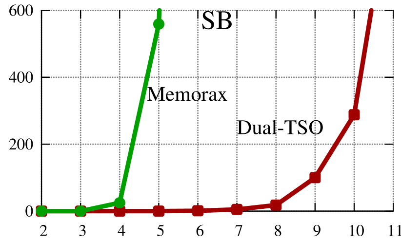
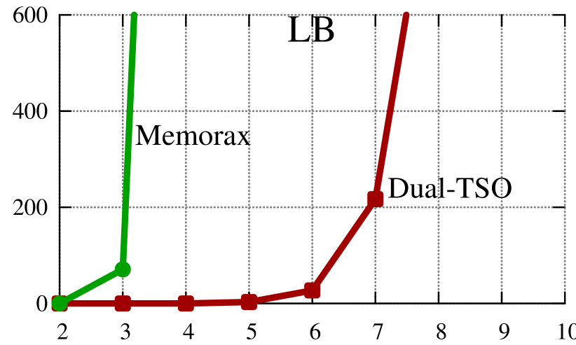
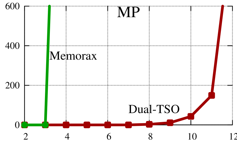
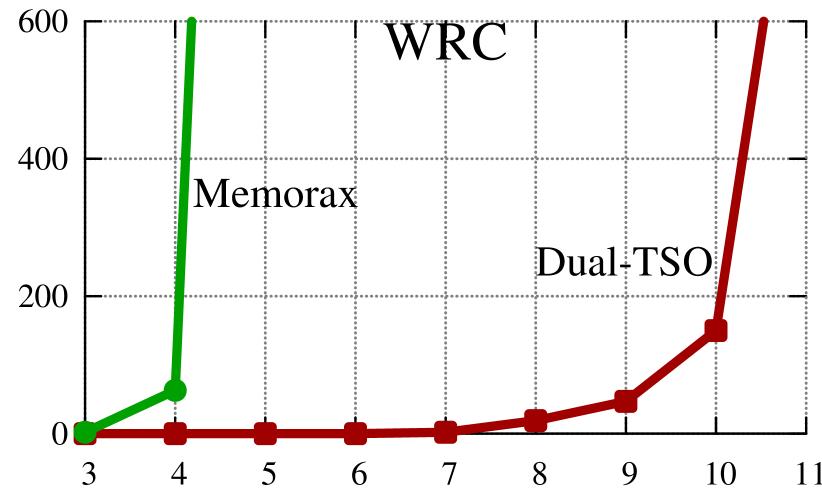
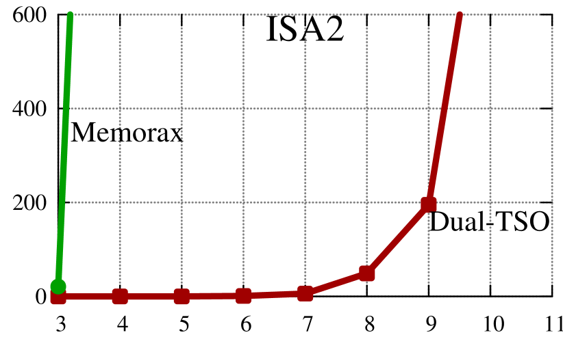
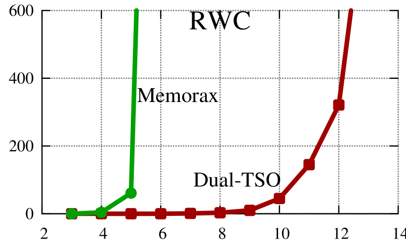
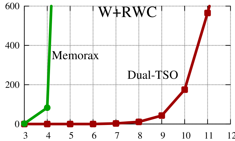
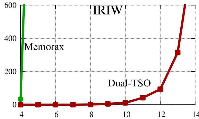
Figure 8. Running time of Memorax and Dual-TSO$(\sqsubseteq)$ by increasing number of processes. The x axis is number of processes and the y axis is running time in seconds.

Program	Safe under TSO	Dual-TSO$(\trianglelefteq)$
		$\mathbf{\#T(s)}$	$\mathbf{\#C}$
SB	no	0.0	147
LB	yes	0.6	1 028
MP	yes	0.0	149
WRC	yes	0.8	618
ISA2	yes	4.3	1 539
RWC	no	0.2	293
W+RWC	no	1.5	828
IRIW	yes	4.6	648

Table 2. Parameterized verification with Dual-TSO$(\trianglelefteq)$.

Verification of Parameterized Concurrent Systems.

The second set compares the scalability of Memorax and Dual-TSO while increasing the number of processes. The results are given in Figure 8. We observe that although the algorithms implemented by Dual-TSO$(\sqsubseteq)$ and Memorax have the same (non-primitive recursive) lower bound (in theory), Dual-TSO$(\sqsubseteq)$ scales better than Memorax in all these benchmarks. In fact, Memorax can only handle benchmarks with at most 5 processes while Dual-TSO can handle benchmarks with more processes. We conjecture that this is due to the important advantages of the Dual TSO semantics. In fact, the Dual TSO semantics transforms the load buffers into lossy channels without adding the costly overhead of memory snapshots that was necessary in the case of Memorax. The absence of this extra overhead means that our tool generates less configurations (due to the ordering) and this results in a better performance and scalability.

Table 2 presents the running time and the number of generated configurations when checking the state reachability problem for the parameterized versions of the benchmarks in Figure 8 with Dual-TSO$(\trianglelefteq)$. It should be emphasized that Dual-TSO$(\trianglelefteq)$ and Dual-TSO$(\sqsubseteq)$ have the same results for the reachability problems in these benchmarks. We observe that the verification of these parameterized systems is much more efficient than verification of bounded-size instances (starting from a number of processes of 3 or 4), especially concerning memory consumption (which is given in terms of number of generated configurations). The reason behind is that the size of the generated minor sets in the analysis of a parameterized system are usually smaller than the size of the generated minor sets during the analysis of an instance of the system with a large number of processes. In fact, during the analysis of a parameterised concurrent system, the number of considered processes in the generated minimal configurations is usually very small. Observe that, in the case of concurrent systems, the number of considered processes in the generated minimal configurations is equal to the number of processes in the given system.

7. Conclusion

In this paper, we have presented an alternative (yet equivalent) semantics to the classical one for the TSO memory model that is more amenable for efficient algorithmic verification and for extension to parametric verification. This new semantics allows us to understand the TSO memory model in a totally different way compared to the classical semantics. Furthermore, the proposed semantics offers several important advantages from the point of view of formal reasoning and program verification. First, the Dual TSO semantics allows transforming the load buffers to lossy channels (in the sense that the processes can lose any message situated at the head of any load buffer in non-deterministic manner) without adding the costly overhead that was necessary in the case of store buffers. This means that we can apply the theory of well-structured systems [Abd10, ACJT96, FS01] in a straightforward manner leading to a much simpler proof of decidability of safety properties. Second, the absence of extra overhead means that we obtain more efficient algorithms and better scalability (as shown by our experimental results). Finally, the Dual TSO semantics allows extending the framework to perform parameterized verification which is an important paradigm in concurrent program verification.

In the future, we plan to apply our techniques to other memory models and to combine with predicate abstraction for handling programs with unbounded data domain.

Appendix A Proof of Theorem 1

We prove the theorem by showing its if direction and then only if direction. In the following, for a TSO (DTSO)-configuration $c=\left({\bf q},{\bf b},{\bf mem}\right)$, we use ${\tt states}\left(c\right)$, ${\tt buffers}\left(c\right)$, and ${\tt mem}\left(c\right)$ to denote ${\bf q}$, ${\bf b}$, and ${\bf mem}$ respectively.

A.1. From Dual TSO to TSO

We show the if direction of Theorem 1. Consider a DTSO-computation

$$\pi_{\sf DTSO}=c_{0}\xrightarrow{t_{1}}_{{\sf DTSO}}c_{1}\xrightarrow{t_{2}}_{{\sf DTSO}}c_{2}\cdots\xrightarrow{t_{n-1}}_{{\sf DTSO}}c_{n-1}\xrightarrow{t_{n}}_{{\sf DTSO}}c_{n}$$

where $c_{0}=c^{D}_{\it init}$ and $c_{i}$ is of the form $\left({\bf q}_{i},{\bf b}_{i},{\bf mem}_{i}\right)$ for all $i:1\leq i\leq n$ with ${\bf q}_{n}={\bf q}_{target}$ and ${\bf b}_{n}(p)=\epsilon$ for all $p\in{\mathbb{P}}$. We will derive a TSO-computation $\pi_{\sf TSO}$ such that ${\it target}\left(\pi_{\sf TSO}\right)$ is a configuration of the form $\left({\tt states}\left(c_{n}\right),{\bf b},{\tt mem}\left(c_{n}\right)\right)$ where ${\bf b}(p)=\epsilon$ for all $p\in{\mathbb{P}}$.

First, we define some functions that we will use in the construction of the computation $\pi_{\sf TSO}$. Then, we define a sequence of TSO-configurations that appear in $\pi_{\sf TSO}$. Finally, we show that the TSO-computation $\pi_{\sf TSO}$ exists. In particular, the target configuration ${\it target}\left(\pi_{\sf TSO}\right)$ has the same local states as the target $c_{n}$ of the DTSO-computation $\pi_{\sf DTSO}$.

Let $1\leq i_{1}<i_{2}<\cdots<i_{k}\leq n$ be the sequence of indices such that $t_{i_{1}}t_{i_{2}}\ldots t_{i_{k}}$ is the sequence of write or atomic read-write operations occurring in the computation $\pi_{\sf DTSO}$. In the following, we assume that $i_{0}=0$.

For each $j:0\leq j\leq n$, we associate a mapping function $\mathsf{index}_{j}:{\mathbb{P}}\rightarrow\{0,\ldots,k\}^{*}$ that associates for each process $p\in{\mathbb{P}}$ and each message at the position $\ell:1\leq\ell\leq|{\tt buffers}\left(c_{j}\right)\left(p\right)|$ in the load buffer ${\tt buffers}\left(c_{j}\right)\left(p\right)$ the index $\mathsf{index}_{j}(p)(\ell)$, i.e., the index of the last write or atomic write-read operations at the moment this message has been added to the load buffer. Formally, we define $\mathsf{index}_{j}$ as follows:

1. $\mathsf{index}_{0}(p):=\epsilon$ for all $p\in{\mathbb{P}}$.

2. Consider j such that $0\leq j<n$. Recall that $c_{j}\xrightarrow{t_{j+1}}_{{\sf DTSO}}c_{j+1}$ with $t_{j+1}\in\Delta_{p}\cup\Delta^{\prime}_{p}$. We define $\mathsf{index}_{j+1}$ based on $\mathsf{index}_{j}$:

   • Nop, read, fence, arw: If $t_{j+1}$ is of the following forms $\left(q,{\sf nop},q^{\prime}\right)$, $\left(q,{\sf r}(x,v),q^{\prime}\right)$, $\left(q,{\sf fence},q^{\prime}\right)$, or $\left(q,{\sf arw}(x,v,v^{\prime}),q^{\prime}\right)$, then $\mathsf{index}_{j+1}:=\mathsf{index_{j}}$.

   • Write: If $t_{j+1}$ is of the form $\left(q,{\sf w}(x,v),q^{\prime}\right)$, then $\mathsf{index}_{j+1}:=\mathsf{index}_{j}\left[p\hookleftarrow r\cdot\mathsf{index}_{j}(p)\right]$ with $i_{r}=j+1$.

   • Propagate: If $t_{j+1}$ is of the form ${\sf propagate}_{p}^{x}$, then $\mathsf{index}_{j+1}:=\mathsf{index}_{j}\left[p\hookleftarrow r\cdot\mathsf{index}_{j}(p)\right]$ where $r:0\leq r\leq k$ is the maximal index such that $i_{r}\leq j+1$.

   • Delete: If $t_{j+1}$ is of the form ${\sf delete}_{p}$, then $\mathsf{index}_{j}:=\mathsf{index}_{j+1}\left[p\hookleftarrow\mathsf{index}_{j+1}(p)\cdot r\right]$ with $r=\mathsf{index}_{j}(p)(|\mathsf{index}_{j}(p)|)$.

Next, we associate for each process $p\in{\mathbb{P}}$ and $j:0\leq j\leq n$, the memory view ${\sf view}_{p}(c_{j})$ of the process $p$ in the configuration $c_{j}$ as follows:

1. If ${\tt buffers}\left(c_{j}\right)\left(p\right)=\epsilon$, then ${\sf view}_{p}(c_{j}):=r$ where $r:0\leq r\leq k$ is the maximal index such that $i_{r}\leq j$.

2. If ${\tt buffers}\left(c_{j}\right)\left(p\right)\neq\epsilon$, then ${\sf view}_{p}(c_{j}):={\mathsf{index}_{j}(p)}(|\mathsf{index_{j}}(p)|)$.

We give an example of how to calculate the functions index and view for a DTSO-computation. Let consider the following DTSO-computation

$$\pi_{\sf DTSO}=c_{0}\xrightarrow{t_{1}}_{{\sf DTSO}}c_{1}\xrightarrow{t_{2}}_{{\sf DTSO}}c_{2}\xrightarrow{t_{3}}_{{\sf DTSO}}c_{3}\xrightarrow{t_{4}}_{{\sf DTSO}}c_{4}\xrightarrow{t_{5}}_{{\sf DTSO}}c_{5}$$

containing only transitions of a process $p$ with two variables $x$ and $y$ where $c_{i}=\left({\bf q}_{i},{\bf b}_{i},{\bf mem}_{i}\right)$ for all $i:0\leq i\leq n=5$ such that:

$${\bf q}_{0}(p) =q_{0}, {\bf b}_{0}(p) =\epsilon, {\bf mem}_{0}(x) =0,{\bf mem}_{0}(y)=0, t_{1} =\left(q_{0},{\sf w}(x,1),q_{1}\right),$$

$${\bf q}_{1}(p) =q_{1}, {\bf b}_{1}(p) =\left(x,1,{\textsc{own}}\right), {\bf mem}_{1}(x) =1,{\bf mem}_{1}(y)=0, t_{2} ={\sf propagate}_{p}^{y},$$

$${\bf q}_{2}(p) =q_{1}, {\bf b}_{2}(p) =(y,0)\cdot\left(x,1,{\textsc{own}}\right), {\bf mem}_{2}(x) =1,{\bf mem}_{2}(y)=0, t_{3} ={\sf delete}_{p},$$

$${\bf q}_{3}(p) =q_{1}, {\bf b}_{3}(p) =(y,0), {\bf mem}_{3}(x) =1,{\bf mem}_{3}(y)=0, t_{4} =(q_{1},{\sf r}(y,0),q_{2}),$$

$${\bf q}_{4}(p) =q_{2}, {\bf b}_{4}(p) =(y,0), {\bf mem}_{4}(x) =1,{\bf mem}_{4}(y)=0, t_{5} ={\sf delete}_{p},$$

$${\bf q}_{5}(p) =q_{2}, {\bf b}_{5}(p) =\epsilon, {\bf mem}_{5}(x) =1,{\bf mem}_{5}(y)=0.$$

We note that $n=5$ and $\pi_{\sf DTSO}$ contains only transitions of the process $p$. We also note that $k=1$ and $i_{1}=1$ is the index of the only write transition $t_{1}$ occurring in the computation $\pi_{\sf DTSO}$. Following the above definitions of index and view, we define the functions index and view as follows:

1. For each $j:0\leq j\leq n=5$, we define the mapping function $\mathsf{index}_{j}(p)$:

   $$\mathsf{index}_{0}(p) =\epsilon, \mathsf{index}_{1}(p) =1, \mathsf{index}_{2}(p) =1.1,$$

   $$\mathsf{index}_{3}(p) =1, \mathsf{index}_{4}(p) =1, \mathsf{index}_{5}(p) =\epsilon.$$

2. For each $j:0\leq j\leq n=5$, we define the memory view ${\sf view}_{p}(c_{j})$:

   $${\sf view}_{p}(c_{0}) =0, {\sf view}_{p}(c_{1}) =1, {\sf view}_{p}(c_{2}) =1,$$

   $${\sf view}_{p}(c_{3}) =1, {\sf view}_{p}(c_{4}) =1, {\sf view}_{p}(c_{5}) =1. \triangle$$

Now, let $\prec$ be an arbitrary total order on the set of processes and let $p_{\it min}$ and $p_{\it max}$ be the smallest and largest elements of $\prec$ respectively. For $p\neq p_{\it max}$, we define $\mathit{succ}(p)$ to be the successor of $p$ wrt. $\prec$, i.e., $p\prec\mathit{succ}(p)$ and there is no $p^{\prime}$ with $p\prec p^{\prime}\prec\mathit{succ}(p)$. We define $\mathit{prev}(p)$ for $p\neq p_{\it min}$ analogously.

The computation $\pi_{\sf TSO}$ will consist of $k+1$ phases (henceforth referred to as the phases $0,1,2,\ldots,k$). In fact, $\pi_{\sf TSO}$ will have the same sequence of memory updates as $\pi_{\sf DTSO}$. At the phase $r$, the computation $\pi_{\sf TSO}$ simulates the movements of the processes where their memory view index is $r$. The order in which the processes are simulated during phase $r$ is defined by the ordering $\prec$. First, process $p_{\it min}$ will perform a sequence of transitions. This sequence is derived from the sequence of transitions it performs in $\pi_{\sf DTSO}$ where its memory view index is $r$, including “no”, write, read, fence transitions. Then, the next process performs its transitions. This continues until $p_{\it max}$ has made all its transitions. When all processes have performed their transitions in phase $r$, we execute exactly one update transition (possibly with a write transition) or one atomic read-write transition in order to move to phase $r+1$. We start the phase $r+1$ by letting $p_{\it min}$ execute its transitions, and so on.

Formally, we define a scheduling function $\alpha(r,p,\ell)$ that gives for each $r:0\leq r\leq k$, $p\in{\mathbb{P}}$, and $\ell\geq 1$ a natural number $j:0\leq j\leq n$ such that process $p$ executes the transition $t_{j}$ as its $\ell^{th}$ transition during phase $r$. The scheduling function $\alpha$ is defined as follows where $r:0\leq r\leq k$, $p\in{\mathbb{P}}$, and $\ell\geq 0$:

1. $\alpha(r,p,\ell+1)$ is defined to be the smallest $j$ such that $\alpha(r,p,\ell)<j$, $t_{j}\in\Delta_{p}$ and ${\sf view}_{p}(c_{j})=r$. Intuitively, the $(\ell+1)^{th}$ transition of process $p$ during phase $r$ is defined by the next transition from $t_{\alpha(r,p,\ell)}$ that belongs to $\Delta_{p}$. Notice that ${\alpha(r,p,\ell+1)}$ is defined only for finitely many $\ell$.

2. If $\{{j}\,|\,{{\sf view}_{p}(c_{j})=r}\}\neq\emptyset$, we define $\alpha(r,p,0):=\mathit{min}\{{j}\,|\,{{\sf view}_{p}(c_{j})=r}\}$. Otherwise, we define $\alpha(r,p,0):=\alpha(r-1,p,\sharp(r-1,p))$ where

   $$\sharp(r,p):=\mathit{max}\{\ell\,|\,\ell\geq 0,\alpha(r,p,\ell)\,\,\,\text{is defined}\}.$$

   Intuitively, phase $r$ starts for process $p$ at the point where its memory view index becomes equal to $r$. Notice that $\alpha(0,p,0)=0$ for all $p\in{\mathbb{P}}$ since all processes are initially in phase $0$.

In the following, we show how to calculate the scheduling function $\alpha(r,p,\ell)$ and $\sharp(r,p)$ where $r:0\leq r\leq k$, $p\in{\mathbb{P}}$, and $\ell\geq 0$ for the DTSO-computation $\pi_{\sf DTSO}$ given in Example A.1. We recall that $k=1$, $n=5$ and the definitions of the two functions index and view are given in Example A.1. We also recall that $\pi_{\sf DTSO}$ contains only transitions of the process $p$. The constructed TSO-computation $\pi_{\sf TSO}$ from $\pi_{\sf DTSO}$ will consist of $k+1=2$ phases, referred as the phase $0$ and the phase $1$. In order to define the transitions of the process $p$ in different phases, for each $r:0\leq r\leq k=1$ and $\ell\geq 0$, the scheduling function $\alpha(r,p,\ell)$ and $\sharp(r,p)$ is defined as follows:

$$\alpha(0,p,0) =0, \alpha(1,p,0) =1, \alpha(1,p,1) =4,$$

$$\sharp(0,p) =0, \sharp(1,p) =1. \triangle$$

In order to define $\pi_{\sf TSO}$, we first define the set of configurations that will appear in $\pi_{\sf TSO}$. In more detail, for each $r:0\leq r\leq k$, $p\in{\mathbb{P}}$, and $\ell:0\leq\ell\leq\sharp(r,p)$, we define a TSO-configuration $d_{r,p,\ell}$ based on the DTSO-configurations that are appearing in $\pi_{\sf DTSO}$. We will define $d_{r,p,\ell}$ by defining its local states, buffer contents, and memory state.

1. We define the local states of the processes as follows:

   • ${\tt states}\left(d_{r,p,\ell}\right)\left(p\right):={\tt states}\left(c_{\alpha(r,p,\ell)}\right)\left(p\right)$. After process $p$ has performed its $\ell^{\it th}$ transition during phase $r$, its local state is identical to its local state in the corresponding DTSO-configuration $c_{\alpha(r,p,\ell)}$.

   • If $p^{\prime}\prec p$ then ${\tt states}\left(d_{r,p,\ell}\right)\left(p^{\prime}\right):={\tt states}\left(c_{\alpha(r,p^{\prime},\sharp\left({r},{p^{\prime}}\right))}\right)\left(p^{\prime}\right)$, i.e. the state of $p^{\prime}$ will not change while $p$ is making its moves. This state is given by the local state of $p^{\prime}$ after it made its last move during phase $r$.

   • If $p\prec p^{\prime}$ then ${\tt states}\left(d_{r,p,\ell}\right)\left(p^{\prime}\right):={\tt states}\left(c_{\alpha(r,p^{\prime},0)}\right)\left(p^{\prime}\right)$, i.e. the local state of $p^{\prime}$ will not change while $p$ is making its moves. This state is given by the local state of $p^{\prime}$ when it entered phase $r$ (before it has made any moves during phase $r$).

2. To define the buffer contents, we give more definitions. For a DTSO-message $a$ of the form $(x,v)$, we define ${\tt DTSO2TSO}\left(a\right)$ to be $\epsilon$. For a DTSO-message $a$ of the form $(x,v,{\textsc{own}})$, we define ${\tt DTSO2TSO}\left(a\right)$ to be $(x,v)$. From that, we define ${\tt DTSO2TSO}\left(\epsilon\right)=\epsilon$ and ${\tt DTSO2TSO}\left(a_{1}a_{2}\cdots a_{n}\right):={\tt DTSO2TSO}\left(a_{1}\right)\cdot{\tt DTSO2TSO}\left(a_{2}\right)\cdots{\tt DTSO2TSO}\left(a_{n}\right)$, i.e., we concatenate the results of applying the operation individually on each $a_{i}$ with $1\leq i\leq n$. We define ${\tt DTSO2TSO_{+}}\left(w\right)$ for a word $w\in\left(({\mathbb{X}}\times{\mathbb{V}})\cup({\mathbb{X}}\times{\mathbb{V}}\times\{\textsc{own}\})\right)^{*}$ as follows: If $|w|=0$ then ${\tt DTSO2TSO_{+}}\left(w\right):=\epsilon$, else ${\tt DTSO2TSO_{+}}\left(w\right):={\tt DTSO2TSO}\left(w(1)w(2)\cdots w(|w|-1)\right)$. In the following, we give the definition of the buffer contents of $d_{r,p,\ell}$:

   • ${\tt buffers}\left(d_{r,p,\ell}\right)\left(p\right):={\tt DTSO2TSO_{+}}\left({\tt buffers}\left(c_{\alpha(r,p,\ell)}\right)\left(p\right)\right)$. After process $p$ has performed its $\ell^{th}$ transition during phase $r$, the content of its buffer is defined by considering the buffer of the corresponding DTSO-configuration $c_{\alpha(r,p,\ell)}$ and only messages belong to $p$ (i.e., of the form $\left(x,v,{\textsc{own}}\right)$).

   • If $p^{\prime}\prec p$ then ${\tt buffers}\left(d_{r,p,\ell}\right)\left(p^{\prime}\right):={\tt buffers}\left(c_{\alpha(r,p^{\prime},\sharp\left({r},{p^{\prime}}\right))}\right)\left(p^{\prime}\right)$. In a similar manner to the case of states, if $p^{\prime}\prec p$ then the buffer of $p^{\prime}$ will not change while $p$ is making its moves.

   • If $p\prec p^{\prime}$ then ${\tt buffers}\left(d_{r,p,\ell}\right)\left(p^{\prime}\right):={\tt buffers}\left(c_{\alpha(r,p^{\prime},0)}\right)\left(p^{\prime}\right)$. In a similar manner to the case of states, if $p\prec p^{\prime}$ then the buffer of $p^{\prime}$ will not be changed while $p$ is making its moves.

3. We define the memory state as follows:

   • ${\tt mem}\left(d_{r,p,\ell}\right):={\tt mem}\left(c_{i_{r}}\right)$. This definition is consistent with the fact that all processes have identical views of the memory when they are in the same phase $r$. This view is defined by the memory component of $c_{i_{r}}$.

In the following, we give the configurations $d_{r,p,\ell}$ for all $r:0\leq r\leq k$, $p\in{\mathbb{P}}$, and $\ell:0\leq\ell\leq\sharp(r,p)$ that will appear in the constructed TSO-computation $\pi_{\sf TSO}$ from $\pi_{\sf DTSO}$ given in Example A.1. We call that $k=1$, $n=5$, and $\pi_{\sf DTSO}$ contains only transitions of the process $p$. We also recall that the scheduling function $\alpha(r,p,\ell)$ and $\sharp(r,p)$ are given in Example A.1.

For each $r:0\leq r\leq k=1$ and $\ell:0\leq\ell\leq\sharp(r,p)$, we define the TSO-configurations $d_{r,p,\ell}=\left({\bf q}_{r,p,\ell},{\bf b}_{r,p,\ell},{\bf mem}_{r,p,\ell}\right)$ based on the DTSO-configurations that are appearing in $\pi_{\sf DTSO}$ as follows:

$$d_{0,p,0} : {\bf q}_{0,p,0}(p) =q_{0}, {\bf b}_{0,p,0}(p) =\epsilon, {\bf mem}_{0,p,0}(x) =0,{\bf mem}_{0,p,0}(y)=0,$$

$$d_{1,p,0} : {\bf q}_{1,p,0}(p) =q_{1}, {\bf b}_{1,p,0}(p) =\epsilon, {\bf mem}_{1,p,0}(x) =1,{\bf mem}_{1,p,0}(y)=0,$$

$$d_{1,p,1} : {\bf q}_{1,p,0}(p) =q_{2}, {\bf b}_{1,p,1}(p) =\epsilon, {\bf mem}_{1,p,1}(x) =1,{\bf mem}_{1,p,1}(y)=0.$$

Finally, we construct the TSO-computation

$$\pi_{\sf TSO}=d_{0,p,0}\xrightarrow{t^{\prime}_{1}}_{\sf TSO}d^{\prime}_{0,p,0}\xrightarrow{t^{\prime}_{2}}_{\sf TSO}d_{1,p,0}\xrightarrow{t^{\prime}_{3}}_{\sf TSO}d_{1,p,1}$$

where

$$d^{\prime}_{0,p,0} =\left({\bf q}^{\prime}_{0,p,0},{\bf b}^{\prime}_{0,p,0},{\bf mem}^{\prime}_{0,p,0}\right),$$

$$t^{\prime}_{1} =\left(q_{0},{\sf w}(x,1),q_{1}\right),$$

$$t^{\prime}_{2} ={\sf update}_{p},$$

$$t^{\prime}_{3} =\left(q_{1},{\sf r}(y,0),q_{2}\right),$$

and:

$$d^{\prime}_{0,p,0} : {\bf q}^{\prime}_{0,p,0}(p) =q_{1}, {\bf b}^{\prime}_{0,p,0}(p) =(x,1), {\bf mem}^{\prime}_{0,p,0}(x) =0,{\bf mem}^{\prime}_{0,p,0}(y)=0.$$

Since there is only one update transition in both two computations $\pi_{\sf DTSO}$ and $\pi_{\sf TSO}$, it is easy to see that $\pi_{\sf TSO}$ has the same sequence of memory updates as $\pi_{\sf DTSO}$. It is also easy to see that $d_{0,p,0}=c_{\it init}$ and $d_{1,p,\sharp\left({1},{p}\right)}=d_{1,p,1}=\left({\tt states}\left(c_{5}\right),{\bf b},{\tt mem}\left(c_{5}\right)\right)$ where ${\bf b}(p)={\tt buffers}\left(c_{5}\right)\left(p\right)=\epsilon$. Therefore, $\pi_{\sf TSO}$ is a witness of the construction.  $\triangle$

The following lemma shows the existence of a TSO-computation $\pi_{\sf TSO}$ that starts from the initial TSO-configuration and whose target has the same local state definitions as the target $c_{n}$ of the DTSO-computation $\pi_{\sf DTSO}$. This concludes the proof of the if direction of Theorem 1.

Lemma 12.

$d_{0,p_{\it min},0}\xrightarrow{\pi_{\sf TSO}}_{\sf TSO}d_{k,p_{\it max},\sharp\left({k},{p_{\it max}}\right)}$ for some TSO-computation $\pi_{\sf TSO}$. Furthermore, $d_{0,p_{\it min},0}$ is the initial TSO-configuration and

$$d_{k,p_{\it max},\sharp\left({k},{p_{\it max}}\right)}=\left({\tt states}\left(c_{n}\right),{\bf b},{\tt mem}\left(c_{n}\right)\right)$$

where ${\tt buffers}\left(p\right)={\tt buffers}\left(c_{n}\right)\left(p\right)=\epsilon$ for all $p\in{\mathbb{P}}$.

Proof A.1.

Lemmas 16–19 show that the existence of the computation $\pi_{\sf TSO}$. Lemma 21 and Lemma 20 show the conditions on the initial and target configurations.

First, we start by establishing Lemma 13, Lemma 14, and Lemma 15 that we will use later.

Lemma 13.

For every $j:0\leq j\leq n$ and process $p\in{\mathbb{P}}$, the following properties hold:

1. $|\mathsf{index}_{j}(p)|=|{\tt buffers}\left(c_{j}\right)\left(p\right)|$.

2. For every $\ell_{1},\ell_{2}:1\leq\ell_{1}\leq\ell_{2}\leq|\mathsf{index}_{j}(p)|$, $\mathsf{index}_{j}(p)(\ell_{2})\leq\mathsf{index}_{j}(p)(\ell_{1})\leq j$.

3. For every $\ell_{1},\ell_{2}:1\leq\ell_{1}<\ell_{2}\leq|\mathsf{index}_{j}(p)|$ such that ${\tt buffers}\left(c_{j}\right)\left(p\right)\left(\ell_{1}\right)$ is of the form $\left(x,v,{\textsc{own}}\right)$, $\mathsf{index}_{j}(p)(\ell_{2})<\mathsf{index}_{j}(p)(\ell_{1})$.

4. For every $\ell:1\leq\ell\leq|{\tt buffers}\left(c_{j}\right)\left(p\right)|$, if $r=\mathsf{index}_{j}(p)(\ell)$ and ${\tt buffers}\left(c_{j}\right)\left(p\right)\left(\ell\right)$ is of the form $\left(x,v,{\textsc{own}}\right)$, then $t_{i_{r}}\in\Delta_{p}$ and it is of the form $\left(q,{\sf w}(x,v),q^{\prime}\right)$.

5. For every $\ell:1\leq\ell\leq|{\tt buffers}\left(c_{j}\right)\left(p\right)|$, if $r=\mathsf{index}_{j}(p)(\ell)$ and ${\tt buffers}\left(c_{j}\right)\left(p\right)\left(\ell\right)$ is of the form $\left(x,v\right)$, then ${\tt mem}\left(c_{i_{r}}\right)\left(x\right)=v$.

6. For every $r_{1},r_{2}:0\leq r_{1}\leq r_{2}\leq k$ such that $r_{1}={\textsc{min}}\{\mathsf{index_{j}(p)(\ell)}\,|\,\ell:1\leq\ell\leq|\mathsf{index}_{j}(p)|\}$, $t_{r_{2}}\in\Delta_{p}$, and $t_{r_{2}}$ is of the form $\left(q,{\sf w}(x,v),q^{\prime}\right)$, then there is an index $\ell:1\leq\ell\leq|\mathsf{index}_{j}(c_{j})(p)|$ such that $\mathsf{index}_{j}(p)(\ell)=r_{2}$ and ${\tt buffers}\left(c_{j}\right)\left(p\right)\left(\ell\right)=\left(x,v,{\textsc{own}}\right)$.

Proof A.2.

The lemma holds following an immediate consequence of the definition of $\mathsf{index}_{j}$.

Lemma 14.

For every process $p\in{\mathbb{P}}$ and index $j:0\leq j<n$, ${\sf view}_{p}(c_{j})\leq{\sf view}_{p}(c_{j+1})$. Furthermore, $i_{{\sf view}_{p}(c_{j})}\leq j$ and $i_{{\sf view}_{p}(c_{j+1})}\leq j+1$.

Proof A.3.

The lemma holds following an immediate consequence of the definitions of ${\sf view}_{p}$ and $\mathsf{index}_{j}$.

Lemma 15.

For every natural number $j$ such that $\alpha(r,p,\ell)\leq j<\alpha(r,p,\ell+1)-1$, ${\tt DTSO2TSO_{+}}\left({\tt buffers}\left(c_{j}\right)\left(p\right)\right)={\tt DTSO2TSO_{+}}\left({\tt buffers}\left(c_{j+1}\right)\left(p\right)\right)$.

Proof A.4.

The proof is done by contradiction. Let us assume that there is some $j:\alpha(r,p,\ell)\leq j<\alpha(r,p,\ell+1)-1$ such that

$${\tt DTSO2TSO_{+}}\left({\tt buffers}\left(c_{j}\right)\left(p\right)\right)\neq{\tt DTSO2TSO_{+}}\left({\tt buffers}\left(c_{j+1}\right)\left(p\right)\right).$$

Observe that the only three operations that can change the content of the load buffer of the process $p$ are write, delete and propagation operations. Since $t_{j}\notin\Delta_{p}$ (and so no write operation has been performed) and propagation will append messages of the form $(x,v)$, this implies that $t_{j}$ is a delete transition of the process $p$ (i.e., $t_{j}={\sf delete}_{p}$). Now, the only case when ${\tt DTSO2TSO_{+}}\left({\tt buffers}\left(c_{j}\right)\left(p\right)\right)\neq{\tt DTSO2TSO_{+}}\left({\tt buffers}\left(c_{j+1}\right)\left(p\right)\right)$ is where ${\tt buffers}\left(c_{j}\right)\left(p\right)$ is of the form $w\cdot(y,v^{\prime},{\textsc{own}})\cdot m$ with $m\in\{(x,v),(x,v,{\textsc{own}})\,|\,x\in{\mathbb{X}},v\in{\mathbb{V}}\}$. This implies that ${\tt buffers}\left(c_{j+1}\right)\left(p\right)=w\cdot(y,v^{\prime},{\textsc{own}})$. Now we can use the third case of Lemma 13 to prove that ${\sf view}_{p}(c_{j+1})>{\sf view}_{p}(c_{j})$. This contradicts the fact that ${\sf view}_{p}(c_{j+1})\leq{\sf view}_{p}(c_{\alpha(r,p,\ell+1)})$ (see Lemma 14) since we have ${\sf view}_{p}(c_{\alpha(r,p,\ell)})={\sf view}_{p}(c_{\alpha(r,p,\ell+1)})=r$ (by definition), ${\sf view}_{p}(c_{j})\geq{\sf view}_{p}(c_{\alpha(r,p,\ell)})$ (see Lemma 14) and ${\sf view}_{p}(c_{j+1})>{\sf view}_{p}(c_{j})$.

Now we can start proving the existence of the computation $\pi_{\sf TSO}$ by showing that we can move from the configuration $d_{r,p,\ell}$ to $d_{r,p,\ell+1}$ using the transition $t_{\alpha(r,p,\ell+1)}$.

Lemma 16.

If $\ell<\sharp\left({r},{p}\right)$ then $d_{r,p,\ell}\xrightarrow{t_{\alpha(r,p,\ell+1)}}_{\sf TSO}d_{r,p,\ell+1}$.

Proof A.5.

We recall that $t_{\alpha(r,p,\ell+1)}\in\Delta_{p}$ by definition. Therefore, $t_{\alpha(r,p,\ell+1)}$ is not a propagation transition nor a delete transition. Furthermore, suppose that $t_{\alpha(r,p,\ell+1)}$ is an atomic read-write transition. It leads to the fact that ${\sf view}_{p}(c_{\alpha(r,p,\ell+1)})>{\sf view}_{p}(c_{\alpha(r,p,\ell)})$, contradicting to the assumption that we are in phase $r$. Hence, $t_{\alpha(r,p,\ell+1)}$ is not an atomic read-write transition.

Let $t_{\alpha(r,p,\ell+1)}\in\Delta_{p}$ be of the form $\left(q,{\it op},q^{\prime}\right)$. To prove the lemma, we will prove the following properties:

1. ${\tt states}\left(d_{\alpha(r,p,\ell)}\right)\left(p\right)=q$ and ${\tt states}\left(d_{r,p,\ell+1}\right)={\tt states}\left(d_{\alpha(r,p,\ell)}\right)\left[p\hookleftarrow q^{\prime}\right]$,

2. ${\tt states}\left(d_{r,p,\ell+1}\right)\left(p^{\prime}\right)={\tt states}\left(d_{r,p,\ell}\right)\left(p^{\prime}\right)$ for $p^{\prime}\neq p$,

3. ${\tt buffers}\left(d_{r,p,\ell+1}\right)\left(p^{\prime}\right)={\tt buffers}\left(d_{r,p,\ell}\right)\left(p^{\prime}\right)$ for $p^{\prime}\neq p$,

4. ${\tt mem}\left(d_{r,p,\ell}\right)={\tt mem}\left(d_{r,p,\ell+1}\right)={\tt mem}\left(c_{i_{r}}\right)$,

5. The contents of ${\tt buffers}\left(d_{r,p,\ell}\right)\left(p\right)$ and ${\tt buffers}\left(d_{r,p,\ell+1}\right)\left(p\right)$ are compatible with the transition $t_{\alpha(r,p,\ell+1)}$. In means that with the properties (1)–(4), the property (5) allows that $d_{r,p,\ell}\xrightarrow{t_{\alpha(r,p,\ell+1)}}_{\sf TSO}d_{r,p,\ell+1}$.

We prove the property (1). We see from definition of $\alpha$ that $t_{j}\not\in\Delta_{p}$ for all $j:\alpha(r,p,\ell)<j<\alpha(r,p,\ell+1)$. It follows that ${\tt states}\left(c_{j}\right)\left(p\right)={\tt states}\left(c_{\alpha(r,p,\ell)}\right)\left(p\right)$ for all $j:\alpha(r,p,\ell)<j<\alpha(r,p,\ell+1)$. In particular, we have ${\tt states}\left(c_{\alpha(r,p,\ell+1)-1}\right)\left(p\right)={\tt states}\left(c_{\alpha(r,p,\ell)}\right)\left(p\right)$. Then, from the fact that $c_{\alpha(r,p,\ell+1)-1}\xrightarrow{t_{\alpha}(r,p,\ell+1)}_{{\sf DTSO}}c_{\alpha(r,p,\ell+1)}$ and the definitions of $d_{r,p,\ell}$ and $d_{r,p,\ell+1}$, we know that ${\tt states}\left(d_{r,p,\ell}\right)\left(p\right)={\tt states}\left(c_{\alpha(r,p,\ell)}\right)\left(p\right)={\tt states}\left(c_{\alpha(r,p,\ell+1)-1}\right)\left(p\right)=q$. It follows that

$${\tt states}\left(d_{r,p,\ell+1}\right)\left(p\right)={\tt states}\left(c_{\alpha(r,p,\ell+1)}\right)\left(p\right)=q^{\prime}.$$

This concludes the property (1).

We prove the property (2). We see from the definitions of $d_{\alpha(r,p,\ell)}$ and $d_{\alpha(r,p,\ell+1)}$ that if $p^{\prime}\prec p$ then ${\tt states}\left(d_{r,p,\ell+1}\right)\left(p^{\prime}\right)={\tt states}\left(c_{\alpha(r,p^{\prime},\sharp\left({k},{p^{\prime}}\right))}\right)\left(p^{\prime}\right)={\tt states}\left(d_{r,p,\ell}\right)\left(p^{\prime}\right)$. Moreover, we have if $p\prec p^{\prime}$ then

$${\tt states}\left(d_{r,p,\ell+1}\right)\left(p^{\prime}\right)={\tt states}\left(c_{\alpha(r,p^{\prime},0)}\right)\left(p^{\prime}\right)={\tt states}\left(d_{r,p,\ell}\right)\left(p^{\prime}\right).$$

This concludes the property (2).

We prove the properties (3) and (4). In a similar manner to the case of states, we can show the property (3). By the definitions of $d_{\alpha(r,p,\ell)}$ and $d_{\alpha(r,p,\ell+1)}$ and the fact that $\ell<\ell+1\leq\sharp\left({r},{p}\right)$, we have ${\tt mem}\left(d_{r,p,\ell}\right)={\tt mem}\left(c_{i_{r}}\right)={\tt mem}\left(d_{r,p,\ell+1}\right)$. This concludes the property (4).

Now, it remains to prove the property (5). We consider the cases where ${\it op}$ is a write or a read operation. The other cases can be treated in a similar way.

• ${\it op}={\sf w}(x,v)$: We see from Lemma 15 that for all: $j:\alpha(r,p,\ell)<j<\alpha(r,p,\ell+1)$

  $${\tt DTSO2TSO_{+}}\left({\tt buffers}\left(c_{\alpha(r,p,\ell)}\right)\left(p\right)\right)={\tt DTSO2TSO_{+}}\left({\tt buffers}\left(c_{j}\right)\left(p\right)\right)$$

  In particular, we have

  $${\tt DTSO2TSO_{+}}\left({\tt buffers}\left(c_{\alpha(r,p,\ell)}\right)\left(p\right)\right)={\tt DTSO2TSO_{+}}\left({\tt buffers}\left(c_{\alpha(r,p,\ell+1)-1}\right)\left(p\right)\right)$$

  Then, since $c_{\alpha(r,p,\ell+1)-1}\xrightarrow{t_{\alpha}(r,p,\ell+1)}_{{\sf DTSO}}c_{\alpha(r,p,\ell+1)}$, we have ${\tt buffers}\left(c_{\alpha(r,p,\ell+1)}\right)\left(p\right)=\left(x,v,{\textsc{own}}\right)\cdot{\tt buffers}\left(c_{\alpha(r,p,\ell+1)-1}\right)\left(p\right)$.

  We will show that ${\tt buffers}\left(c_{\alpha(r,p,\ell+1)-1}\right)\left(p\right)\neq\epsilon$ by contradiction. Let us suppose that ${\tt buffers}\left(c_{\alpha(r,p,\ell+1)-1}\right)\left(p\right)=\epsilon$. By definition, we have ${\sf view}_{p}(c_{\alpha(r,p,\ell+1)})=r^{\prime}$ such that $i_{r^{\prime}}={\alpha(r,p,\ell+1)}$. Furthermore, by applying Lemma 14 to $c_{\alpha(r,p,\ell)}$, we know that $i_{r}\leq{\alpha(r,p,\ell)}$. Then, since $\alpha(r,p,\ell)<\alpha(r,p,\ell+1)$ by definition, we have $i_{r}<i_{r^{\prime}}$. This contradicts to the fact that ${\sf view}_{p}(c_{\alpha(r,p,\ell+1)})=r$ by definition. Therefore, we have ${\tt buffers}\left(c_{\alpha(r,p,\ell+1)-1}\right)\left(p\right)\neq\epsilon$.

  As a consequence of the fact that ${\tt buffers}\left(c_{\alpha(r,p,\ell+1)-1}\right)\left(p\right)\neq\epsilon$, we know that

  $${\tt DTSO2TSO_{+}}\left({\tt buffers}\left(c_{\alpha(r,p,\ell+1)}\right)\left(p\right)\right)=(x,v)\cdot{\tt DTSO2TSO_{+}}\left({\tt buffers}\left(c_{\alpha(r,p,\ell)-1}\right)\left(p\right)\right)$$

  Then, since

  $${\tt DTSO2TSO_{+}}\left({\tt buffers}\left(c_{\alpha(r,p,\ell)}\right)\left(p\right)\right)={\tt DTSO2TSO_{+}}\left({\tt buffers}\left(c_{\alpha(r,p,\ell+1)-1}\right)\left(p\right)\right),$$

  it follows that ${\tt buffers}\left(d_{r,p,\ell+1}\right)=(x,v)\cdot{\tt buffers}\left(d_{r,p,\ell}\right)$. Hence this implies that $d_{r,p,\ell}\xrightarrow{t_{\alpha(r,p,\ell+1)}}_{\sf TSO}d_{r,p,\ell+1}$.

• ${\it op}={\sf r}(x,v)$: We see from Lemma 15 that for all $j:\alpha(r,p,\ell)<j<\alpha(r,p,\ell+1)$

  $${\tt DTSO2TSO_{+}}\left({\tt buffers}\left(c_{\alpha(r,p,\ell)}\right)\left(p\right)\right)={\tt DTSO2TSO_{+}}\left({\tt buffers}\left(c_{j}\right)\left(p\right)\right)$$

  In particular, we have

  $${\tt DTSO2TSO_{+}}\left({\tt buffers}\left(c_{\alpha(r,p,\ell)}\right)\left(p\right)\right)={\tt DTSO2TSO_{+}}\left({\tt buffers}\left(c_{\alpha(r,p,\ell+1)-1}\right)\left(p\right)\right)$$

  Then, since $c_{\alpha(r,p,\ell+1)-1}\xrightarrow{t_{\alpha}(r,p,\ell+1)}_{{\sf DTSO}}c_{\alpha(r,p,\ell+1)}$, we have ${\tt buffers}\left(c_{\alpha(r,p,\ell+1)}\right)\left(p\right)={\tt buffers}\left(c_{\alpha(r,p,\ell+1)-1}\right)\left(p\right)$. Therefore, ${\tt buffers}\left(d_{r,p,\ell+1}\right)\left(p\right)={\tt buffers}\left(d_{r,p,\ell}\right)\left(p\right)$. We consider two cases about the type of the operation ${\it op}$:

  • Read own write: We see that there is an $i:1\leq i<|{\tt buffers}\left(c_{\alpha(r,p,\ell+1)-1}\right)\left(p\right)|$ such that ${\tt buffers}\left(c_{\alpha(r,p,\ell+1)-1}\right)\left(p\right)\left(i\right)=\left(x,v,{\textsc{own}}\right)$, and that there are no $j:1\leq j<i$ and $v^{\prime}\in{\mathbb{V}}$ such that ${\tt buffers}\left(c_{\alpha(r,p,\ell+1)-1}\right)\left(p\right)\left(j\right)=\left(x,v^{\prime},{\textsc{own}}\right)$. As a consequence, this implies that there is an $i^{\prime}:1\leq i^{\prime}\leq|{\tt DTSO2TSO_{+}}\left({\tt buffers}\left(c_{\alpha(r,p,\ell+1)-1}\right)\left(p\right)\right)|$ such that ${\tt DTSO2TSO_{+}}\left({\tt buffers}\left(c_{\alpha(r,p,\ell+1)-1}\right)\left(p\right)\left(i^{\prime}\right)\right)=\left(x,v\right)$ and there are no $j^{\prime}:1\leq j^{\prime}<i^{\prime}$ and $v^{\prime}\in{\mathbb{V}}$ such that ${\tt DTSO2TSO_{+}}\left({\tt buffers}\left(c_{\alpha(r,p,\ell+1)-1}\right)\left(p\right)\left(j\right)\right)=\left(x,v^{\prime}\right)$. From the fact that

    $${\tt buffers}\left(d_{r,p,\ell+1}\right)\left(p\right)={\tt buffers}\left(d_{r,p,\ell}\right)\left(p\right)={\tt DTSO2TSO_{+}}\left({\tt buffers}\left(c_{\alpha(r,p,\ell+1)-1}\right)\right),$$

    we have $d_{r,p,\ell}\xrightarrow{t_{\alpha(r,p,\ell+1)}}_{\sf TSO}d_{r,p,\ell+1}.$

  • Read memory: We consider two cases:

    1. ${\tt buffers}\left(c_{\alpha(r,p,\ell+1)-1}\right)\left(p\right)\left(i\right)=\left(x,v,{\textsc{own}}\right)$ where $i=|{\tt buffers}\left(c_{\alpha(r,p,\ell+1)-1}\right)\left(p\right)|$ and there are no $j:1\leq j<i$ and $v^{\prime}\in{\mathbb{V}}$ such that ${\tt buffers}\left(c_{\alpha(r,p,\ell+1)-1}\right)\left(p\right)\left(j\right)=\left(x,v^{\prime},{\textsc{own}}\right)$: Since ${\sf view}_{p}(c_{\alpha(r,p,\ell+1)-1})=r$, this implies from Lemma 13 that $t_{i_{r}}\in\Delta_{p}$ and it is of the form $\left(q,{\sf w}(x,v),q^{\prime}\right)$. Hence, we see that ${\tt mem}\left(c_{i_{r}}\right)\left(x\right)=v$ and thus ${\tt mem}\left(d_{r,p,\ell}\right)\left(x\right)={\tt mem}\left(d_{r,p,\ell+1}\right)\left(x\right)=v$. Therefore, we have $d_{r,p,\ell}\xrightarrow{t_{\alpha(r,p,\ell+1)}}_{\sf TSO}d_{r,p,\ell+1}$.

    2. $\left(x,v^{\prime},{\textsc{own}}\right)\not\in{\tt buffers}\left(c_{\alpha(r,p,\ell+1)-1}\right)\left(p\right)$ for all $v^{\prime}\in{\mathbb{V}}$: Thus ${\tt buffers}\left(c_{\alpha(r,p,\ell+1)-1}\right)$ is of the form $w\cdot(x,v)$. Since ${\sf view}_{p}(c_{\alpha(r,p,\ell+1)-1})=r$, this implies from Lemma 13 that ${\tt mem}\left(c_{i_{r}}\right)\left(x\right)=v$ and thus ${\tt mem}\left(d_{r,p,\ell}\right)\left(x\right)={\tt mem}\left(d_{r,p,\ell+1}\right)\left(x\right)=v$. Therefore, we have $d_{r,p,\ell}\xrightarrow{t_{\alpha(r,p,\ell+1)}}_{\sf TSO}d_{r,p,\ell+1}$.

This concludes the proof of Lemma 16.

Lemma 17.

If $p\prec p_{\it max}$ then $d_{r,p,\sharp\left({r},{p}\right)}=d_{r,{\it succ}\left(p\right),0}$.

Proof A.6.

To prove the lemma, we will prove the following properties:

1. ${\tt states}\left(d_{r,p,\sharp\left({r},{p}\right)}\right)\left(p^{\prime}\right)={\tt states}\left(d_{r,{\it succ}\left(p\right),0}\right)\left(p^{\prime}\right)$ for all $p^{\prime}\in{\mathbb{P}}$,

2. ${\tt buffers}\left(d_{r,p,\sharp\left({r},{p}\right)}\right)\left(p^{\prime}\right)={\tt buffers}\left(d_{r,{\it succ}\left(p\right),0}\right)\left(p^{\prime}\right)$ for all $p^{\prime}\in{\mathbb{P}}$,

3. ${\tt mem}\left(d_{r,p,\sharp\left({r},{p}\right)}\right)={\tt mem}\left(d_{r,{\it succ}\left(p\right),0}\right)$.

We prove the property (1) by considering four cases:

• $p^{\prime}=p$: From the definitions of $d_{r,{\it succ}\left(p\right),\ell}$ and $d_{r,p,\sharp\left({r},{p}\right)}$, we have ${\tt states}\left(d_{r,{\it succ}\left(p\right),\ell}\right)\left(p\right)={\tt states}\left(d_{r,p,\sharp\left({r},{p}\right)}\right)\left(p\right)$ for all $\ell:0\leq\ell\leq\sharp\left({r},{{\it succ}\left(p\right)}\right)$. In particular, we see that ${\tt states}\left(d_{r,{\it succ}\left(p\right),0}\right)\left(p\right)={\tt states}\left(d_{r,p,\sharp\left({r},{p}\right)}\right)\left(p\right)$.

• $p^{\prime}={\it succ}\left(p\right)$: From the definitions of $d_{r,p,\ell}$ and $d_{r,{\it succ}\left(p\right),0}$, ${\tt states}\left(d_{r,p,\ell}\right)\left({\it succ}\left(p\right)\right)={\tt states}\left(d_{r,{\it succ}\left(p\right),0}\right)\left({\it succ}\left(p\right)\right)$ for all $\ell:0\leq\ell\leq\sharp\left({r},{p}\right)$. In particular, we see that ${\tt states}\left(d_{r,p,\sharp\left({r},{p}\right)}\right)\left({\it succ}\left(p\right)\right)={\tt states}\left(d_{r,{\it succ}\left(p\right),0}\right)\left({\it succ}\left(p\right)\right)$. It follows from $p^{\prime}={\it succ}\left(p\right)$ that ${\tt states}\left(d_{r,p,\sharp\left({r},{p}\right)}\right)\left(p^{\prime}\right)={\tt states}\left(d_{r,{\it succ}\left(p\right),0}\right)\left(p^{\prime}\right)$.

• $p^{\prime}\prec p\prec{\it succ}\left(p\right)$: From the definitions of $d_{r,{\it succ}\left(p\right),\ell}$ and $d_{r,p^{\prime},\sharp\left({r},{p^{\prime}}\right)}$, we know that ${\tt states}\left(d_{r,{\it succ}\left(p\right),\ell}\right)\left(p^{\prime}\right)={\tt states}\left(d_{r,p^{\prime},\sharp\left({r},{p^{\prime}}\right)}\right)\left(p^{\prime}\right)$ for all $\ell:0\leq\ell\leq\sharp\left({r},{{\it succ}\left(p\right)}\right)$. In particular, we see that ${\tt states}\left(d_{r,{\it succ}\left(p\right),0}\right)\left(p^{\prime}\right)={\tt states}\left(d_{r,p^{\prime},\sharp\left({r},{p^{\prime}}\right)}\right)\left(p^{\prime}\right)$. Also, by a similar argument, we have ${\tt states}\left(d_{r,p,\ell}\right)\left(p^{\prime}\right)={\tt states}\left(d_{r,p^{\prime},\sharp\left({r},{p^{\prime}}\right)}\right)\left(p^{\prime}\right)$ for all $\ell:0\leq\ell\leq\sharp\left({r},{p}\right)$. In particular, we see that ${\tt states}\left(d_{r,p,\sharp\left({r},{p}\right)}\right)\left(p^{\prime}\right)={\tt states}\left(d_{r,p^{\prime},\sharp\left({r},{p^{\prime}}\right)}\right)\left(p^{\prime}\right)$. Hence, we have ${\tt states}\left(d_{r,{\it succ}\left(p\right),0}\right)\left(p^{\prime}\right)={\tt states}\left(d_{r,p,\sharp\left({r},{p}\right)}\right)\left(p^{\prime}\right)$.

• $p\prec{\it succ}\left(p\right)\prec p^{\prime}$: From the definitions of $d_{r,{\it succ}\left(p\right),\ell}$ and $d_{r,p^{\prime},0}$, we can see that ${\tt states}\left(d_{r,{\it succ}\left(p\right),\ell}\right)\left(p^{\prime}\right)={\tt states}\left(d_{r,p^{\prime},0}\right)\left(p^{\prime}\right)$ for all $\ell:0\leq\ell\leq\sharp\left({r},{p}\right)$. In particular, we see that ${\tt states}\left(d_{r,{\it succ}\left(p\right),0}\right)\left(p^{\prime}\right)={\tt states}\left(d_{r,p^{\prime},0}\right)\left(p^{\prime}\right)$. Also, by a similar argument, we have ${\tt states}\left(d_{r,p,\ell}\right)\left(p^{\prime}\right)={\tt states}\left(d_{r,p^{\prime},0}\right)\left(p^{\prime}\right)$ for all $\ell:0\leq\ell\leq\sharp\left({r},{p}\right)$. In particular, we see that ${\tt states}\left(d_{r,p,\sharp\left({r},{p}\right)}\right)\left(p^{\prime}\right)={\tt states}\left(d_{r,p^{\prime},0}\right)\left(p^{\prime}\right)$. Hence, we have ${\tt states}\left(d_{r,{\it succ}\left(p\right),0}\right)\left(p^{\prime}\right)={\tt states}\left(d_{r,p,\sharp\left({r},{p}\right)}\right)\left(p^{\prime}\right)$.

We prove the properties (2) and (3). By a similar manner to the case of states, we can show the property (2). Finally, to show the property (3), by the definition of $d_{r,p,\sharp\left({r},{p}\right)}$, it follows that ${\tt mem}\left(d_{r,p,\sharp\left({r},{p}\right)}\right)={\tt mem}\left(c_{i_{r}}\right)$. Also, by a similar argument, we have ${\tt mem}\left(d_{r,{\it succ}\left(p\right),0}\right)={\tt mem}\left(c_{i_{r}}\right)$. Hence, we have ${\tt mem}\left(d_{r,p,\sharp\left({r},{p}\right)}\right)={\tt mem}\left(d_{r,{\it succ}\left(p\right),0}\right)$.

This concludes the proof of Lemma 17.

Lemma 18.

If $r<k$ and $t_{i_{r+1}}\in\Delta_{p^{u}}$ such that $t_{i_{r+1}}$ is of the form $\left(q,{\sf arw}(x,v,v^{\prime}),q^{\prime}\right)$, then $d_{r,p_{\it max},\sharp\left({r},{p_{\it max}}\right)}\xrightarrow{t_{{i}_{r+1}}}_{\sf TSO}d_{r+1,p_{\it min},0}$.

Proof A.7.

To prove the lemma, we will prove the following properties:

1. ${\tt states}\left(d_{r,p_{\it max},\sharp\left({r},{p_{\it max}}\right)}\right)\left(p\right)={\tt states}\left(d_{r+1,p_{\it min},0}\right)\left(p\right)$ for all $p\neq p^{u}$,

2. ${\tt buffers}\left(d_{r,p_{\it max},\sharp\left({r},{p_{\it max}}\right)}\right)\left(p\right)={\tt buffers}\left(d_{r+1,p_{\it min},0}\right)\left(p\right)$ for all $p\neq p^{u}$,

3. ${\tt states}\left(d_{r,p_{\it max},\sharp\left({r},{p_{\it max}}\right)}\right)\left(p^{u}\right)=q$, and ${\tt states}\left(d_{r+1,p_{\it min},0}\right)\left(p^{u}\right)=q^{\prime}$,

4. ${\tt buffers}\left(d_{r,p_{\it max},\sharp\left({r},{p_{\it max}}\right)}\right)\left(p^{u}\right)={\tt buffers}\left(d_{r+1,p_{\it min},0}\right)\left(p^{u}\right)=\epsilon$,

5. ${\tt mem}\left(d_{r,p_{\it max},\sharp\left({r},{p_{\it max}}\right)}\right)\left(x\right)=v$ and ${\tt mem}\left(d_{r+1,p_{\it min},0}\right)\left(x\right)=v^{\prime}$.

We show the property (1). Let $p\in{\mathbb{P}}\setminus\left\{p^{u}\right\}$. From the definition of $d_{r,p_{\it max},\sharp\left({r},{p_{\it max}}\right)}$ and $d_{r,p,\sharp\left({r},{p}\right)}$, ${\tt states}\left(d_{r,p_{\it max},\sharp\left({r},{p_{\it max}}\right)}\right)\left(p\right)={\tt states}\left(d_{r,p,\sharp\left({r},{p}\right)}\right)\left(p\right)={\tt states}\left(c_{\alpha(r,p,\sharp\left({r},{p}\right))}\right)\left(p\right)$ and ${\tt states}\left(d_{r+1,p_{\it min},0}\right)\left(p\right)={\tt states}\left(d_{r+1,p,0}\right)\left(p\right)={\tt states}\left(c_{\alpha(r+1,p,0)}\right)\left(p\right)$. From the definition of $\alpha$, it follows that $t_{j}\not\in\Delta_{p}$ for all $j:\alpha(r,p,\sharp\left({r},{p}\right))\leq j<\alpha(r+1,p,0)$. This implies that ${\tt states}\left(c_{\alpha(r+1,p,0)-1}\right)\left(p\right)={\tt states}\left(c_{\alpha(r,p,\sharp\left({r},{p}\right))}\right)\left(p\right)$. Now we have two cases:

• $\{{j}\,|\,{{\sf view}_{p}(c_{j})=r+1}\}=\emptyset$: We see that $\alpha(r+1,p,0)=\alpha(r,p,\sharp\left({r},{p}\right))$, and hence that ${\tt states}\left(d_{r,p_{\it max},\sharp\left({r},{p_{\it max}}\right)}\right)\left(p\right)={\tt states}\left(d_{r+1,p_{\it min},0}\right)\left(p\right)$.

• $\{{j}\,|\,{{\sf view}_{p}(c_{j})=r+1}\}\neq\emptyset$: Since ${\sf view}_{p}(c_{\alpha(r+1,p,0)-1})=r$, we can show that $t_{\alpha(r+1,p,0)}\notin\Delta_{p}$. This is done by contradiction as follows. In fact if $t_{\alpha(r+1,p,0)}\in\Delta_{p}$, then it is either a write transition or an atomic read-write transition. This implies that in both cases that ${\tt buffers}\left(c_{\alpha(r+1,p,0)-1}\right)\left(p\right)=\epsilon$ and that ${\sf view}_{p}(c_{\alpha(r+1,p,0)})=\alpha(r+1,p,0)$. Hence, we have $\alpha(r+1,p,0)=r+1$, and this leads to a contradiction since $t_{i_{r+1}}\in\Delta_{p^{u}}$. Thus, we have ${\tt states}\left(d_{r,p_{\it max},\sharp\left({r},{p_{\it max}}\right)}\right)\left(p\right)={\tt states}\left(d_{r+1,p_{\it min},0}\right)\left(p\right)$.

In a similar manner to the case of states, we can show the property (2). Now we show the properties (3) and (4). Using a similar reasoning as for the process $p$, we know that ${\tt states}\left(c_{\alpha(r+1,p^{u},0)-1}\right)\left(p^{u}\right)={\tt states}\left(c_{\alpha(r,p^{u},\sharp\left({r},{p^{u}}\right))}\right)\left(p^{u}\right)$. From the definition of $\pi_{\sf DTSO}$, it follows that $c_{\alpha(r+1,p^{u},0)-1}\xrightarrow{t_{\alpha(r+1,p^{u},0)}}_{{\sf DTSO}}c_{\alpha(r+1,p^{u},0)}$. Furthermore, since ${\sf view}_{p}(c_{\alpha(r+1,p^{u},0)})=r+1$ and ${\sf view}_{p}(c_{\alpha(r+1,p^{u},0)-1})<r+1$, we know that $t_{\alpha(r+1,p^{u},0)}=t_{i_{r+1}}$. This implies that ${\tt buffers}\left(c_{\alpha(r+1,p^{u},0)-1}\right)\left(p^{u}\right)={\tt buffers}\left(c_{\alpha(r+1,p^{u},0)}\right)\left(p^{u}\right)=\epsilon$ and ${\tt states}\left(c_{\alpha(r+1,p^{u},0)-1}\right)\left(p^{u}\right)=q$ and ${\tt states}\left(c_{\alpha(r+1,p^{u},0)}\right)\left(p^{u}\right)=q^{\prime}$. Now since

$${\tt DTSO2TSO_{+}}\left({\tt buffers}\left(c_{\alpha(r,p^{u},\sharp\left({r},{p^{u}}\right))}\right)\left(p^{u}\right)\right)={\tt DTSO2TSO_{+}}\left({\tt buffers}\left(c_{\alpha(r+1,p^{u},0)-1}\right)\left(p^{u}\right)\right),$$

we see that

$${\tt buffers}\left(d_{r,p_{\it max},\sharp\left({r},{p_{\it max}}\right)}\right)\left(p^{u}\right)={\tt buffers}\left(d_{r+1,p_{\it min},0}\right)\left(p^{u}\right)=\epsilon$$

and that ${\tt states}\left(d_{r,p_{\it max},\sharp\left({r},{p_{\it max}}\right)}\right)\left(p^{u}\right)=q$ and ${\tt states}\left(d_{r+1,p_{\it min},0}\right)\left(p^{u}\right)=q^{\prime}$. This concludes the properties (3) and (4).

We show the property (5). From the definition of $\pi_{\sf DTSO}$, it follows that ${\tt mem}\left(c_{i_{r+1}}\right)={\tt mem}\left(c_{i_{r}}\right)\left[x\hookleftarrow v^{\prime}\right]$ with ${\tt mem}\left(c_{i_{r}}\right)\left(x\right)=v$. Then from the definitions of $d_{r,p_{\it max},\sharp\left({r},{p_{\it max}}\right)}$ and $d_{r+1,p_{\it min},0}$, we have the property (5).

This concludes the proof of Lemma 18.

Lemma 19.

If $r<k$ and $t_{i_{r+1}}\in\Delta_{p^{u}}$ such that $t_{i_{r+1}}$ is of the form $\left(q,{\sf w}(x,v),q^{\prime}\right)$, then $d_{r,p_{\it max},\sharp\left({r},{p_{\it max}}\right)}\xrightarrow{*}_{\sf TSO}d_{r+1,p_{\it min},0}$.

Proof A.8.

To prove the lemma, we will prove the following properties:

1. ${\tt states}\left(d_{r,p_{\it max},\sharp\left({r},{p_{\it max}}\right)}\right)\left(p\right)={\tt states}\left(d_{r+1,p_{\it min},0}\right)\left(p\right)$ for all $p\neq p^{u}$,

2. ${\tt buffers}\left(d_{r,p_{\it max},\sharp\left({r},{p_{\it max}}\right)}\right)\left(p\right)={\tt buffers}\left(d_{r+1,p_{\it min},0}\right)\left(p\right)$ for all $p\neq p^{u}$,

3. The contents of buffers ${\tt states}\left(d_{r,p_{\it max},\sharp\left({r},{p_{\it max}}\right)}\right)\left(p^{u}\right)$ and ${\tt states}\left(d_{r+1,p_{\it min},0}\right)\left(p^{u}\right)$ are compatible, i.e. with the properties (1)–(2), the property (3) allows $d_{r,p_{\it max},\sharp\left({r},{p_{\it max}}\right)}\xrightarrow{*}_{\sf TSO}d_{r+1,p_{\it min},0}$.

We show the property (1). Let $p\in{\mathbb{P}}\setminus\left\{p^{u}\right\}$. From the definitions of $d_{r,p_{\it max},\sharp\left({r},{p_{\it max}}\right)}$ and $d_{r,p,\sharp\left({r},{p}\right)}$, ${\tt states}\left(d_{r,p_{\it max},\sharp\left({r},{p_{\it max}}\right)}\right)\left(p\right)={\tt states}\left(d_{r,p,\sharp\left({r},{p}\right)}\right)\left(p\right)={\tt states}\left(c_{\alpha(r,p,\sharp\left({r},{p}\right))}\right)\left(p\right)$ and that ${\tt states}\left(d_{r+1,p_{\it min},0}\right)\left(p\right)={\tt states}\left(d_{r+1,p,0}\right)\left(p\right)={\tt states}\left(c_{\alpha(r+1,p,0)}\right)\left(p\right)$. From the definition of $\alpha$, it follows that $t_{j}\not\in\Delta_{p}$ for all $j:\alpha(r,p,\sharp\left({r},{p}\right))\leq j<\alpha(r+1,p,0)$. This implies that ${\tt states}\left(c_{\alpha(r+1,p,0)-1}\right)\left(p\right)={\tt states}\left(c_{\alpha(r,p,\sharp\left({r},{p}\right))}\right)\left(p\right)$. Now we have two cases:

• $\{{j}\,|\,{{\sf view}_{p}(c_{j})=r+1}\}=\emptyset$: We see that $\alpha(r+1,p,0)=\alpha(r,p,\sharp\left({r},{p}\right))$, and hence that ${\tt states}\left(d_{r,p_{\it max},\sharp\left({r},{p_{\it max}}\right)}\right)\left(p\right)={\tt states}\left(d_{r+1,p_{\it min},0}\right)\left(p\right)$.

• $\{{j}\,|\,{{\sf view}_{p}(c_{j})=r+1}\}\neq\emptyset$: Since ${\sf view}_{p}(c_{\alpha(r+1,p,0)-1})=r$, we can show that $t_{\alpha(r+1,p,0)}\notin\Delta_{p}$ . This is done by contradiction as follows. In fact if $t_{\alpha(r+1,p,0)}\in\Delta_{p}$, then it is either a write transition or an atomic read-write transition. This implies that in both cases that ${\tt buffers}\left(c_{\alpha(r+1,p,0)-1}\right)\left(p\right)=\epsilon$ and that ${\sf view}_{p}(c_{\alpha(r+1,p,0)})=\alpha(r+1,p,0)$. Hence, we have $\alpha(r+1,p,0)=r+1$, and this leads to a contradiction since $t_{i_{r+1}}\in\Delta_{p^{u}}$. Thus, we have ${\tt states}\left(d_{r,p_{\it max},\sharp\left({r},{p_{\it max}}\right)}\right)\left(p\right)={\tt states}\left(d_{r+1,p_{\it min},0}\right)\left(p\right)$.

In a similar manner to the case of states, we can show the property (2). Now we show the property (3). Using a similar reasoning as for the process $p$, we know that ${\tt states}\left(c_{\alpha(r+1,p^{u},0)-1}\right)\left(p^{u}\right)={\tt states}\left(c_{\alpha(r,p^{u},\sharp\left({r},{p^{u}}\right))}\right)\left(p^{u}\right)$. From the definition of $\pi_{\sf DTSO}$, it follows that $c_{\alpha(r+1,p^{u},0)-1}\xrightarrow{t_{\alpha(r+1,p^{u},0)}}_{{\sf DTSO}}c_{\alpha(r+1,p^{u},0)}$. Furthermore, from the fact that ${\sf view}_{p}(c_{\alpha(r+1,p^{u},0)})=r+1$ and ${\sf view}_{p}(c_{\alpha(r+1,p^{u},0)-1})<r+1$, we have two cases to consider:

• ${\tt buffers}\left(c_{\alpha(r+1,p^{u},0)-1}\right)\left(p^{u}\right)=\epsilon$: It follows from the conditions for ${\sf view}_{p}(c_{\alpha(r+1,p^{u},0)})$ and ${\sf view}_{p}(c_{\alpha(r+1,p^{u},0)-1})$ that $t_{\alpha(r+1,p^{u},0)}=t_{i_{r+1}}$, ${\tt buffers}\left(c_{\alpha(r+1,p^{u},0)}\right)\left(p^{u}\right)=(x,v,{\textsc{own}})$, and that ${\tt states}\left(c_{\alpha(r+1,p^{u},0)-1}\right)\left(p^{u}\right)=q$ and ${\tt states}\left(c_{\alpha(r+1,p^{u},0)}\right)\left(p^{u}\right)=q^{\prime}$. From

  $${\tt DTSO2TSO_{+}}\left({\tt buffers}\left(c_{\alpha(r,p^{u},\sharp\left({r},{p^{u}}\right))}\right)\left(p^{u}\right)\right)={\tt DTSO2TSO_{+}}\left({\tt buffers}\left(c_{\alpha(r+1,p^{u},0)-1}\right)\left(p^{u}\right)\right)$$

  we have ${\tt buffers}\left(d_{r,p_{\it max},\sharp\left({r},{p_{\it max}}\right)}\right)\left(p^{u}\right)={\tt buffers}\left(d_{r+1,p_{\it min},0}\right)\left(p^{u}\right)=\epsilon$. Moreover, we have ${\tt states}\left(d_{r,p_{\it max},\sharp\left({r},{p_{\it max}}\right)}\right)\left(p^{u}\right)=q$, and ${\tt states}\left(d_{r+1,p_{\it min},0}\right)\left(p^{u}\right)=q^{\prime}$. Then, it is easy to see that ${\tt mem}\left(c_{i_{r+1}}\right)={\tt mem}\left(c_{i_{r}}\right)\left[x\hookleftarrow v\right]$. Hence, we have $d_{r,p_{\it max},\sharp\left({r},{p_{\it max}}\right)}\xrightarrow{t_{{i}_{r+1}}}_{\sf TSO}d^{\prime}\xrightarrow{{{\sf update}_{p^{u}}}}_{\sf TSO}d_{r+1,p_{\it min},0}$ for some configuration $d^{\prime}$.

• ${\tt buffers}\left(c_{\alpha(r+1,p^{u},0)-1}\right)\left(p^{u}\right)\neq\epsilon$: It follows from the conditions for ${\sf view}_{p}(c_{\alpha(r+1,p^{u},0)})$ and ${\sf view}_{p}(c_{\alpha(r+1,p^{u},0)-1})$ that $t_{\alpha(r+1,p^{u},0)}$ is a delete transition of the process $p^{u}$. As a consequence, ${\tt buffers}\left(c_{\alpha(r+1,p^{u},0)-1}\right)\left(p^{u}\right)=w\cdot(x,v,{\textsc{own}})\cdot m$ and ${\tt buffers}\left(c_{\alpha(r+1,p^{u},0)}\right)\left(p^{u}\right)=w\cdot(x,v,{\textsc{own}})$. Hence, we see that

  $${\tt DTSO2TSO_{+}}\left({\tt buffers}\left(c_{\alpha(r+1,p^{u},0)}\right)\left(p^{u}\right)\right)={\tt DTSO2TSO_{+}}\left({\tt buffers}\left(c_{\alpha(r+1,p^{u},0)-1}\right)\left(p^{u}\right)\right)\cdot(x,v)$$

  and therefore ${\tt buffers}\left(d_{r+1,p_{\it min},0}\right)\left(p^{u}\right)={\tt buffers}\left(d_{r,p_{\it max},\sharp\left({r},{p_{\it max}}\right)}\right)\left(p^{u}\right)(x,v)$. Furthermore, we have ${\tt states}\left(c_{\alpha(r+1,p^{u},0)}\right)\left(p^{u}\right)={\tt states}\left(c_{\alpha(r+1,p^{u},0)-1}\right)\left(p^{u}\right)$ and this implies that ${\tt states}\left(d_{r,p_{\it max},\sharp\left({r},{p_{\it max}}\right)}\right)\left(p^{u}\right)={\tt states}\left(d_{r+1,p_{\it min},0}\right)\left(p^{u}\right)$. Then, it is easy to see that ${\tt mem}\left(c_{i_{r+1}}\right)={\tt mem}\left(c_{i_{r}}\right)\left[x\hookleftarrow v\right]$. Hence, we have $d_{r,p_{\it max},\sharp\left({r},{p_{\it max}}\right)}\xrightarrow{{{\sf update}_{p^{u}}}}_{\sf TSO}d_{r+1,p_{\it min},0}$.

This concludes the proof of Lemma 19.

The following lemma shows that the TSO-computation $\pi_{\sf TSO}$ starts from the initial TSO-configuration.

Lemma 20.

$d_{0,p_{\it min},0}$ is the initial TSO-configuration.

Proof A.9.

Let us take any $p\in{\mathbb{P}}$. By the definitions of $d_{0,p_{\it min},0}$, $d_{0,p,0}$, and $\alpha(0,p,0)$, it follows that ${\tt states}\left(d_{0,p_{\it min},0}\right)\left(p\right)={\tt states}\left(d_{0,p,0}\right)\left(p\right)={\tt states}\left(c_{\alpha(0,p,0)}\right)\left(p\right)={\tt states}\left(c_{0}\right)\left(p\right)={\bf q_{\it init}}$. Also, ${\tt buffers}\left(d_{0,p_{\it min},0}\right)\left(p\right)={\tt buffers}\left(d_{0,p,0}\right)\left(p\right)={\tt DTSO2TSO_{+}}\left({\tt buffers}\left(c_{0}\right)\left(p\right)\right)=\epsilon$. Finally, we have ${\tt mem}\left(d_{0,p_{\it min},0}\right)={\tt mem}\left(c_{i_{0}}\right)={\tt mem}\left(c_{0}\right)$. The result follows immediately for the definition of the initial TSO-configuration. This concludes the proof of Lemma 20.

The following lemma shows that the target of the TSO-computation $\pi_{\sf TSO}$ has the same local process states as the target $c_{n}$ of the DTSO-computation $\pi_{\sf DTSO}$.

Lemma 21.

${\tt states}\left(d_{k,p_{\it max},\sharp\left({k},{p_{\it max}}\right)}\right)={\tt states}\left(c_{n}\right)$.

Proof A.10.

Let us take any $p\in{\mathbb{P}}$. By the definitions of $d_{k,p_{\it max},\sharp\left({k},{p_{\it max}}\right)}$ and $d_{k,p,\sharp\left({k},{p}\right)}$, it follows that ${\tt states}\left(d_{k,p_{\it max},\sharp\left({k},{p_{\it max}}\right)}\right)\left(p\right)={\tt states}\left(d_{k,p,\sharp\left({k},{p}\right)}\right)\left(p\right)={\tt states}\left(c_{\alpha(k,p,\sharp\left({k},{p}\right))}\right)\left(p\right)$. By definition of $\alpha(k,p,\sharp\left({k},{p}\right))$, we know that $t_{j}\not\in\Delta_{p}$ for all $j:\alpha(k,p,\sharp\left({k},{p}\right))<j\leq n$. Therefore, we have ${\tt states}\left(c_{j}\right)\left(p\right)={\tt states}\left(c_{n}\right)\left(p\right)$ for all $j:\alpha(k,p,\sharp\left({k},{p}\right))\leq j<n$. In particular, we have ${\tt states}\left(c_{\alpha(k,p,\sharp\left({k},{p}\right))}\right)\left(p\right)={\tt states}\left(c_{n}\right)\left(p\right)$. Hence, we have ${\tt states}\left(d_{k,p_{\it max},\sharp\left({r},{p_{\it max}}\right)}\right)\left(p\right)={\tt states}\left(c_{n}\right)\left(p\right)$. This concludes the proof of Lemma 21.

A.2. From TSO to Dual TSO

We show the only if direction of Theorem 1. Consider a TSO-computation

$$\pi_{\sf TSO}=c_{0}\xrightarrow{t_{1}}_{\sf TSO}c_{1}\xrightarrow{t_{2}}_{\sf TSO}c_{2}\;\cdots\;\xrightarrow{t_{n-1}}_{\sf TSO}c_{n-1}\xrightarrow{t_{n}}_{\sf TSO}c_{n}.$$

where $c_{0}=c_{\it init}$ and $c_{i}$ is of the form $\left({\bf q}_{i},{\bf b}_{i},{\bf mem}_{i}\right)$ for all $i:1\leq i\leq n$ with ${\bf q}_{n}={\bf q}_{target}$. In the following, we will derive a DTSO-computation $\pi_{\sf DTSO}$ such that ${\tt states}\left({\it target}\left(\pi_{\sf DTSO}\right)\right)={\tt states}\left(c_{n}\right)$, i.e. the runs $\pi_{\sf TSO}$ and $\pi_{\sf DTSO}$ reach the same set of local states at the end of the runs.

Similar to the previous case, we will first define some functions that we will use in the construction of the computation $\pi_{\sf DTSO}$. Then, we define a sequence of DTSO-configurations that appear in $\pi_{\sf DTSO}$. Finally, we show that the DTSO-computation $\pi_{\sf DTSO}$ exists. In particular, the target configuration ${\it target}\left(\pi_{\sf DTSO}\right)$ has the same local states as the target $c_{n}$ of the TSO-computation $\pi_{\sf TSO}$.

For every $p\in{\mathbb{P}}$, let $\Delta_{p}^{{\sf w,arw}}\subseteq\Delta_{p}$ (resp. $\Delta_{p}^{{\sf u,arw}}\subseteq\Delta_{p}\cup\{{\sf update}_{p}\}$) be the set of write (resp. update) and atomic read-write transitions that can be performed by process $p$. Let $\Delta^{\sf r}_{p}$ be the set of read transitions that can be performed by $p$.

Let $I=i_{1}\ldots i_{m}$ be the maximal sequence of indices such that $1\leq i_{1}<i_{2}<\cdots<i_{m}\leq n$ and for every $j:1\leq j\leq m$, we have $t_{i_{j}}$ is an update transition or an atomic read-write transition (i.e., $t_{i_{j}}\in{\bigcup_{p\in{\mathbb{P}}}\,\Delta_{p}^{\sf u,arw}}$). In the following, we assume that $i_{0}=0$. Let $I_{p}$ be the maximal subsequence of $I$ such that all transitions with indices in $I_{p}$ belong to process $p$.

Let $I^{\prime}=i^{\prime}_{1}\ldots i^{\prime}_{m}$ be the maximal sequence of indices such that $1\leq i^{\prime}_{1}<i^{\prime}_{2}<\cdots<i^{\prime}_{m}\leq n$ and for every $j:1\leq j\leq m$, we have $t_{i^{\prime}_{j}}$ is a write transition or an atomic read-write transition (i.e., $t_{i^{\prime}_{j}}\in{\bigcup_{p\in{\mathbb{P}}}\,\Delta_{p}^{\sf w,arw}}$). Let $I^{\prime}_{p}$ be the maximal subsequence of $I^{\prime}$ such that all transitions with indices in $I^{\prime}_{p}$ belong to process $p$. Observe that $|I_{p}|=|I^{\prime}_{p}|$.

For every $j:1\leq j\leq m$, let ${\tt proc}\left(j\right)$ be the process that has the update or atomic read-write transition $t_{i_{j}}$ where $i_{j}\in I$. We define ${\tt match}\left(i_{j}\right)$ to be the index of the write (resp. atomic read-write) transition $t_{{\tt match}\left(i_{j}\right)}$ that corresponds to the update (resp. atomic read-write) transition $t_{i_{j}}$. Formally, ${\tt match}\left(i_{j}\right)$:=$l$ where $\exists k:1\leq k\leq|I_{p}|,I_{p}(k)=i_{j}$, $I^{\prime}_{p}(k)=l$ and $1\leq l\leq n$. Observe that if $t_{i_{j}}$ is an atomic read-write operation, then ${\tt match}\left(i_{j}\right)=i_{j}$.

We give an example of how to calculate the function match for a TSO-computation. Let us consider the following TSO-computation

$$\pi_{\sf TSO}=c_{0}\xrightarrow{t_{1}}_{\sf TSO}c_{1}\xrightarrow{t_{2}}_{\sf TSO}c_{2}\xrightarrow{t_{3}}_{\sf TSO}c_{3}$$

containing only transitions of a process $p$ with two variables $x$ and $y$ where $c_{i}=\left({\bf q}_{i},{\bf b}_{i},{\bf mem}_{i}\right)$ for all $i:0\leq i\leq n=3$ such that:

$${\bf q}_{0}(p) =q_{0}, {\bf b}_{0}(p) =\epsilon, {\bf mem}_{0}(x) =0,{\bf mem}_{0}(y)=0, t_{1} =\left(q_{0},{\sf w}(x,1),q_{1}\right),$$

$${\bf q}_{1}(p) =q_{1}, {\bf b}_{1}(p) =(x,1), {\bf mem}_{1}(x) =0,{\bf mem}_{1}(y)=0, t_{2} ={\sf update}_{p},$$

$${\bf q}_{2}(p) =q_{1}, {\bf b}_{2}(p) =\epsilon, {\bf mem}_{2}(x) =1,{\bf mem}_{2}(y)=0, t_{3} =\left(q_{1},{\sf r}(y,0),q_{2}\right),$$

$${\bf q}_{3}(p) =q_{2}, {\bf b}_{3}(p) =\epsilon, {\bf mem}_{3}(x) =1,{\bf mem}_{3}(y)=0.$$

Following the above definitions of $I$ and $I^{\prime}$, $I=i_{1}=2$ (hence, $m=1$) is the maximal sequence of indices of all update or atomic read-write transitions in $\pi_{\sf TSO}$. In a similar way, $I^{\prime}=i^{\prime}_{1}=1$ is the maximal sequence of indices of all write or atomic read-write transitions in $\pi_{\sf TSO}$. We note that $t_{i_{1}}=t_{2}$ is an update transition, and $t^{\prime}_{i^{\prime}_{1}}=t_{1}$ is a write transition. Since the TSO-computation contains only transition of the process $p$, it follows that $I=I_{p}$ and $I^{\prime}=I^{\prime}_{p}$. Following the above definition of match, with $m=1$ and $n=3$, we have ${\tt match}\left(i_{1}\right)={\tt match}\left(2\right)=1$.  $\triangle$

For every $j:1\leq j\leq n$ such that $t_{j}\in\Delta_{p}^{\sf r}$ is a read transition of process $p$, we define ${\sf fromMem}(t_{j})$ as a predicate such that ${\sf fromMem}(t_{j})$ holds if and only if $(x,v^{\prime})\notin{\tt buffers}\left(c_{j-1}\right)$ for all $v^{\prime}\in{\mathbb{V}}$.

For every $j:1\leq j\leq n$ and $p\in{\mathbb{P}}$, we define the function ${\sf label}_{p}(j)$ as follows:

1. ${\sf label}_{p}(j):=(x,v)$ if $t_{j}\in\Delta_{p}^{r}$ is of the form $(q,{\sf r}(x,v),q^{\prime})$ and ${\sf fromMem}(t_{j})$ holds.

2. ${\sf label}_{p}(j):=(x,v,{\textsc{own}})$ if $t_{j}={\sf update}_{p}$ and ${\tt match}\left(j\right)=l$ with $t_{l}$ of the form $(q,{\sf w}(x,v),q^{\prime})$.

3. ${\sf label}_{p}(j):=\epsilon$ otherwise.

Given a sequence $\ell_{1}\cdots\ell_{k}$ with $k\geq 1$ and $1\leq\ell_{i}\leq n$ for all $i:1\leq i\leq k$, we define ${\sf label}_{p}(\ell_{1}\cdots\ell_{k}):={\sf label}_{p}(\ell_{1})\cdots{\sf label}_{p}(\ell_{k-1})\cdot{\sf label}_{p}(\ell_{k})$. Let ${\sf label}^{\sf rev}_{p}(\ell_{1}\cdots\ell_{k})$ with $k\geq 1$ and $1\leq\ell_{i}\leq n$ for all $i:1\leq i\leq k$ be the reversed string of ${\sf label}_{p}(\ell_{1}\cdots\ell_{k})$, i.e. ${\sf label}^{\sf rev}_{p}(\ell_{1}\cdots\ell_{k}):={\sf label}_{p}(\ell_{k})\cdot{\sf label}_{p}(\ell_{k-1})\cdots{\sf label}_{p}(\ell_{1})$.

In the following, we give an example of how to calculate the functions fromMem and label for the TSO-computation $\pi_{\sf TSO}$ given in Example A.2. We recall that $n=3$ and the function match is given in Example A.2. We also note that $t_{3}$ is the only read transition in $\pi_{\sf TSO}$. Following the above definition of fromMem, we have that ${\tt fromMem}(t_{3})$ holds. Then following the definition of match, for every $j:1\leq j\leq n=3$, we define the function ${\tt label}_{p}(j)$ as follows:

$${\tt label}_{p}(1) =\epsilon, {\tt label}_{p}(2) =(x,1,{\it own}), {\tt label}_{p}(3) =(y,0). \triangle$$

Below we show how to simulate all transitions of the TSO-computation $\pi_{\sf TSO}$ by a set of corresponding transitions in the DTSO-computation $\pi_{\sf DTSO}$. The idea is to divide the DTSO-computation to $m+1$ phases. For $0\leq r<m$, each phase $r$ will end at the configuration $d_{r+1}$ by the simulation of the transition $t_{{\tt match}\left(i_{r+1}\right)}$ in $\pi_{\sf TSO}$. Moreover, in phase $r:0\leq r<m$, we call the process ${\tt proc}\left(r+1\right)$ as the active process, and other processes as the inactive ones. We execute only the DTSO-transitions of the active process $p={\tt proc}\left(r+1\right)$ in its active phases. For other processes $p^{\prime}\neq p$, we only change the content of their buffers in the active phases of $p$. In the final phase $r=m$, all processes will be considered to be active because the index ${i_{m+1}}$ is not defined in the definition of the sequence $I$. The DTSO-computation $\pi_{\sf DTSO}$ will end at the configuration $d_{m+1}$.

For every $r:-1\leq r<m$ and $p\in{\mathbb{P}}$, we define the function ${\tt pos}\left(r,p\right)$ in an inductive way on $r$:

1. ${\tt pos}\left(-1,p\right):=0$ for all $p\in{\mathbb{P}}$.

2. ${\tt pos}\left(r,p\right):={\tt pos}\left(r-1,p\right)$ for all $p\neq{\tt proc}\left(r+1\right)$ and $0\leq r<m$.

3. ${\tt pos}\left(r,p\right):={\tt match}\left(i_{r+1}\right)$ for $p={\tt proc}\left(r+1\right)$ and $0\leq r<m$.

In other words, the function ${\tt pos}\left(r,p\right)$ is the index of the last simulated transition by process $p$ at the end of phase $r$ in the computation $\pi_{\sf TSO}$. Moreover, we use ${\tt pos}\left(-1,p\right)$ to be the index of the starting transition of process $p$ before phase $0$.

In the following, we give an example of how to calculate the function pos for the TSO-computation $\pi_{\sf TSO}$ given in Example A.2. We recall that $m=1$ and $\pi_{\sf TSO}$ contains only transitions of the process $p$. We also recall that the function match is given in Example A.2. Following the above definition of pos, for every $r:-1\leq r<m=1$, we define the function ${\tt pos}\left(r,p\right)$ as follows:

$${\tt pos}\left(-1,p\right) =0, {\tt pos}\left(0,p\right) =1. \triangle$$

Let $d_{0}=c^{D}_{\it init}=\left({\bf q_{\it init}},{\bf b_{\it init}},{\bf mem}_{\it init}\right)$. We define the sequence of DTSO-configurations $d_{1},\ldots,d_{m},d_{m+1}$ by defining their local states, buffer contents, and memory states as follows:

1. For every configuration $d_{r+1}$ where $0\leq r<m$:

   • ${\tt states}\left(d_{r+1}\right)\left(p\right):={\tt states}\left(c_{{\tt pos}\left(r,p\right)}\right)\left(p\right)$,

   • ${\tt mem}\left(d_{r+1}\right):={\tt mem}\left(c_{i_{r+1}}\right)$,

   • ${\tt buffers}\left(d_{r+1}\right)\left(p\right):={\sf label}^{\sf rev}_{p}({{\tt pos}\left(r,p\right)+1}\cdots{i_{r+1}})$.

2. For the final configuration $d_{m+1}$:

   • ${\tt states}\left(d_{m+1}\right)\left(p\right):={\tt states}\left(c_{n}\right)\left(p\right)$,

   • ${\tt mem}\left(d_{m+1}\right):={\tt mem}\left(c_{n}\right)$,

   • ${\tt buffers}\left(d_{m+1}\right)\left(p\right):=\epsilon$.

In the following, we give an example of how to calculate the sequence of configurations $d_{1},\ldots,d_{m},d_{m+1}$ that will appear in the constructed DTSO-computation $\pi_{\sf DTSO}$ from the TSO-computation $\pi_{\sf TSO}$ given in Figure A.2. We recall that $m=1$, $n=3$, and the TSO-computation $\pi_{\sf TSO}$ contains only transitions of the process $p$. We also recall that the functions $\tt label$ and pos are given in Example A.2 and Example A.2, respectively.

The DTSO-computation $\pi_{\sf DTSO}$ will consist of $m+1=2$ phases, referred as the phase $0$ and the phase $1$. For each $r:0\leq r\leq m+1=2$, we define the DTSO-configuration $d_{r}=({\bf q}^{\prime}_{r},{\bf b}^{\prime}_{r},{\bf mem}^{\prime}_{r})$ based on the TSO-configurations that are appearing in $\pi_{\sf TSO}$ as follows:

$$d_{0} : {\bf q}^{\prime}_{0}(p) =q_{0}, {\bf b}^{\prime}_{0}(p) =\epsilon, {\bf mem}^{\prime}_{0}(x) =0,{\bf mem}^{\prime}_{0}(y)=0,$$

$$d_{1} : {\bf q}^{\prime}_{1}(p) =q_{1}, {\bf b}^{\prime}_{1}(p) =(x,1,{\it own}), {\bf mem}^{\prime}_{1}(x) =1,{\bf mem}^{\prime}_{1}(y)=0,$$

$$d_{2} : {\bf q}^{\prime}_{2}(p) =q_{2}, {\bf b}^{\prime}_{1}(p) =\epsilon, {\bf mem}^{\prime}_{2}(x) =1,{\bf mem}^{\prime}_{2}(y)=0.$$

Finally, we construct the DTSO-computation as follows:

$$\pi_{\sf DTSO}=d_{0}\xrightarrow{t^{\prime}_{1}}_{{\sf DTSO}}d_{1}\xrightarrow{t^{\prime}_{2}}_{{\sf DTSO}}d_{12}\xrightarrow{t^{\prime}_{3}}_{{\sf DTSO}}d_{13}\xrightarrow{t^{\prime}_{4}}_{{\sf DTSO}}d_{14}\xrightarrow{t^{\prime}_{5}}_{{\sf DTSO}}d_{2}$$

where $d_{12}=({\bf q}^{\prime}_{12},{\bf b}^{\prime}_{12},{\bf mem}_{12})$, $d_{13}=({\bf q}_{13},{\bf b}^{\prime}_{13},{\bf mem}_{13})$, $d_{14}=({\bf q}^{\prime}_{14},{\bf b}^{\prime}_{14},{\bf mem}_{14})$, $t^{\prime}_{1}=(q_{0},{\sf w}(x,1),q_{1})$, $t^{\prime}_{2}={\sf propagate}_{p}^{y}$, $t^{\prime}_{3}={\sf delete}_{p}$ $t^{\prime}_{4}=(q_{1},{\sf r}(y,0),q_{2})$, $t^{\prime}_{5}={\sf delete}_{p}$, and:

$$d_{12} : {\bf q}^{\prime}_{12}(p) =q_{1}, {\bf b}^{\prime}_{12}(p) =(y,0)\cdot(x,1,{\it own}), {\bf mem}^{\prime}_{12}(x) =1,{\bf mem}^{\prime}_{12}(y)=0,$$

$$d_{13} : {\bf q}^{\prime}_{13}(p) =q_{1}, {\bf b}^{\prime}_{13}(p) =(y,0), {\bf mem}^{\prime}_{13}(x) =1,{\bf mem}^{\prime}_{13}(y)=0,$$

$$d_{14} : {\bf q}^{\prime}_{14}(p) =q_{2}, {\bf b}^{\prime}_{14}(p) =(y,0), {\bf mem}^{\prime}_{14}(x) =1,{\bf mem}^{\prime}_{14}(y)=0.$$

Since there is only one update transition in $\pi_{\sf DTSO}$ and $\pi_{\sf TSO}$, it is easy to see that $\pi_{\sf TSO}$ has the same sequence of memory updates as $\pi_{\sf DTSO}$. It is also easy to see that $d_{0}=c^{D}_{\it init}$ and $d_{3}=\left({\tt states}\left(c_{3}\right),{\bf b},{\tt mem}\left(c_{3}\right)\right)$ where ${\bf b}(p):=\epsilon$. Therefore $\pi_{\sf DTSO}$ is a witness of the construction.  $\triangle$

Lemma 22 shows the existence of a DTSO-computation $\pi_{\sf DTSO}$ that starts from the initial TSO-configuration and whose target has the same local state definitions as the target $c_{n}$ of the TSO-computation $\pi_{\sf TSO}$. The only if direction of Theorem 1 will follow directly from Lemma 22. This concludes the proof of the only if direction of Theorem 1.

Lemma 22.

The following properties hold for the constructed sequence $d_{1},\ldots,d_{m},d_{m+1}$:

• For every $r:0\leq r<m$, $d_{r}\xrightarrow{*}_{{\sf DTSO}}d_{r+1}$,

• $d_{m}\xrightarrow{*}_{{\sf DTSO}}d_{m+1}$.

Proof A.11.

We show the proof of the lemma follows directly Lemma 23 and Lemma 27. To make the proof understandable, below we consider a ${\sf fence}$ transition $t=\left(q,{\sf fence},q^{\prime}\right)$ such that $c\xrightarrow{t}_{\sf TSO}c^{\prime}$ for some $c,c^{\prime}$ as an atomic read-write transition of the form $\left(q,{\sf arw}(x,v,v),q^{\prime}\right)$ where $v\in{\mathbb{V}}$ is the memory value of variable $x\in{\mathbb{X}}$ in $c$. For a given TSO-computation $\pi_{\sf TSO}$, we can calculate such value $v$ for each ${\sf fence}$ transition $\pi_{\sf TSO}$.

Lemma 23.

If $0\leq r<m$, then $d_{r}\xrightarrow{*}_{{\sf DTSO}}d_{r+1}$.

Proof A.12.

We are in phase $r$. Because from the configuration $d_{r}$, the memory has not been changed until the transition $t_{i_{r+1}}$, we observe that all memory-read transitions of the process $p$ between transitions $t_{i_{r}}$ and $t_{i_{r+1}}$ will get values from ${\tt mem}\left(d_{r}\right)$ where $p\in{\mathbb{P}}$. Therefore, we can execute a sequence of propagation transitions to propagate from the memory to the buffer of process $p$ to full fill it by all messages that will satisfy all memory-read transitions of $p$ between $t_{i_{r}}$ and $t_{i_{r+1}}$. We propagate to processes according to the order $\prec$: first to the process $p_{\it min}$ and last to the process $p_{\it max}$. We have the following sequence: $d_{r}\xrightarrow{({\Delta^{\sf propagate}})^{*}}_{{\sf DTSO}}{d_{r}^{p_{\it min}}}\cdots\xrightarrow{(\Delta^{\sf propagate})^{*}}_{{\sf DTSO}}{d_{r}^{p_{\it max}}}$. The shape of the configuration $d_{r}^{p_{\it max}}$ is:

• ${\tt states}\left(d_{r}^{p_{\it max}}\right)\left(p\right)={\tt states}\left(c_{{\tt pos}\left(r-1,p\right)}\right)\left(p\right)$,

• ${\tt mem}\left(d_{r}^{p_{\it max}}\right)={\tt mem}\left(c_{i_{r}}\right)$,

• ${\tt buffers}\left(d_{r}^{p_{\it max}}\right)\left(p\right)={\sf label}^{\sf rev}_{p}({{\tt pos}\left(r-1,p\right)+1}\cdots{i_{r+1}-1})$.

Below let $p={\tt proc}\left(r+1\right)$ be the active process in phase $r$ of the DTSO-computation. For each transition $t$ in the sequence of transitions (including updates) of the active process, $seq$=$(t_{{\tt pos}\left(r-1,p\right)+1}\cdots t_{{\tt match}\left(i_{r+1}\right)})|_{\Delta_{{\tt proc}\left(r+1\right)}\cup\left\{{\sf update}_{{\tt proc}\left(r+1\right)}\right\}}$, we execute a set of transitions in the DTSO-computation as follows:

• To simulate a memory-read transition, we execute the same read transition. And then we execute a delete transition to delete the oldest message in the buffer of ${\tt proc}\left(r+1\right)$.

• To simulate a read-own-write transition, we execute the same read transition.

• To simulate a write transition, we execute the same write transition. This transition must be the transition $t_{{\tt match}\left(i_{r+1}\right)}$. According to Dual TSO semantics, we add an own-message to the buffer of ${\tt proc}\left(r+1\right)$.

• To simulate an ${\sf arw}$ transition, we execute the same atomic read-write transition. This transition must be the transition $t_{{\tt match}\left(i_{r+1}\right)}$ and ${\tt match}\left(i_{r+1}\right)=i_{r+1}$.

• To simulate an update transition, we execute a delete transition to delete the oldest message in the buffer of ${\tt proc}\left(r+1\right)$.

• To simulate a ${\sf nop}$ transition, we execute the same transitions in the DTSO-computation.

Let $\beta(r,l)$ indicate the index in the TSO-computation of the $l^{th}$ transition in the sequence $seq$ where $1\leq l\leq|seq|$. Formally, we define $\beta(r,l):=j$ where $1\leq j\leq n$, $t_{j}\in(\Delta_{p}\cup\left\{{\sf update}_{p}\right\})$ and $seq(l)=t_{j}$. Let configuration $d_{r,l}$ where $0\leq r<m$ be the DTSO-configuration before simulating the transition with the index $\beta(r,l)$. We define $d_{r,l}$ by defining its local states, buffer contents, and memory state:

• ${\tt states}\left(d_{r,l}\right)\left(p\right)$=${\tt states}\left(c_{{\tt pos}\left(r-1,p\right)}\right)\left(p\right)$ for all inactive process $p$ and all $l:1\leq l\leq|seq|$,

• ${\tt states}\left(d_{r,l}\right)\left(p\right)={\tt states}\left(c_{\beta(r,l)-1}\right)\left(p\right)$ for the active process $p$ and all $l:1\leq l\leq|seq|$,

• ${\tt mem}\left(d_{r,l}\right)={\tt mem}\left(c_{i_{r}}\right)$ for the active process $p$ and all $l:1\leq l\leq|seq|$,

• ${\tt buffers}\left(d_{r,l}\right)\left(p\right)$=${\sf label}^{\sf rev}_{p}({{\tt pos}\left(r-1,p\right)+1}\cdots{i_{r+1}-1})$ for all inactive process $p$ and all $l:1\leq l\leq|seq|$,

• ${\tt buffers}\left(d_{r,l}\right)\left(p\right)$=${\sf label}^{\sf rev}_{p}({\beta(r,l)}\cdots{i_{r+1}-1})$ for the active process $p$ and all $l:1\leq l\leq|seq|$.

The Lemma 24, Lemma 26, and Lemma 25 imply the result. More precisely, it shows the existence of a DTSO-computation that starts from the DTSO-configuration $d^{pmax}_{r}$ and whose target is the configuration $d_{r+1}$. This concludes the proof of Lemma 23.

Lemma 24.

$d_{r,1}$= $d_{r}^{p_{\it max}}$ for $0\leq r<m$.

Proof A.13.

We show that $d_{r,1}$ and $d_{r}^{p_{\it max}}$ have the same local states, memory, and buffer contents. We consider two cases for the active and inactive processes.

• For inactive process $p\neq{\tt proc}\left(r+1\right)$, it is easy to see that:

  • ${\tt states}\left(d_{r,1}\right)\left(p\right)={\tt states}\left(c_{{\tt pos}\left(r-1,p\right)}\right)\left(p\right)={\tt states}\left(d^{pmax}_{r}\right)\left(p\right)$ by the definitions of configurations $d_{r,1}$ and $d^{pmax}_{r}$.

  • ${\tt buffers}\left(d_{r,1}\right)\left(p\right)$=${\sf label}^{\sf rev}_{p}({{\tt pos}\left(r-1,p\right)+1}\cdots{i_{r+1}-1})={\tt buffers}\left(d^{pmax}_{r}\right)\left(p\right)$ by the definitions of configurations $d_{r,1}$ and $d^{pmax}_{r}$.

• For the active process $p={\tt proc}\left(r+1\right)$:

  • ${\tt states}\left(d_{r,1}\right)\left(p\right)={\tt states}\left(c_{\beta(r,1)-1}\right)\left(p\right)={\tt states}\left(c_{{\tt pos}\left(r-1,p\right)}\right)\left(p\right)$ by the definition of $\beta(r,1)$. Therefore ${\tt states}\left(d_{r,1}\right)\left(p\right)={\tt states}\left(d^{pmax}_{r}\right)\left(p\right)$.

  • ${\tt buffers}\left(d_{r,1}\right)\left(p\right)$=${\sf label}^{\sf rev}_{p}({\beta(r,1)}\cdots{i_{r+1}-1})$ = ${\sf label}^{\sf rev}_{p}({{\tt pos}\left(r-1,p\right)+1}\cdots{i_{r+1}-1})$ by the definition of $\beta(r,1)$. Therefore ${\tt buffers}\left(d_{r,1}\right)\left(p\right)$ = ${\tt buffers}\left(d^{pmax}_{r}\right)\left(p\right)$.

In both cases, for the memory, ${\tt mem}\left(d_{r,1}\right)={\tt mem}\left(c_{i_{r}}\right)={\tt mem}\left(d^{pmax}_{r}\right)$ by the definitions of configurations $d_{r,1}$ and $d^{pmax}_{r}$.

This concludes the proof of Lemma 24.

Lemma 25.

$d_{r,|seq|}\xrightarrow{t_{{\tt match}\left(i_{r+1}\right)}}_{{\sf DTSO}}d_{r+1}$ for $0\leq r<m$.

Proof A.14.

To prove the lemma, we will show the following properties:

1. $\exists d^{\prime}_{r+1}:d_{r,|seq|}\xrightarrow{t_{{\tt match}\left(i_{r+1}\right)}}_{{\sf DTSO}}d^{\prime}_{r+1}$, i.e. the transition $t_{{\tt match}\left(i_{r+1}\right)}$ is feasible from the configuration $d_{r,|seq|}$.

2. Moreover, $d^{\prime}_{r+1}$=$d_{r+1}$.

Let $p={\tt proc}\left(r+1\right)$ be the active process. We show the property (1) by considering two cases:

• ${\tt match}\left(i_{r+1}\right)$ is a write transition: By simulation, we execute the same transition in the DTSO-computation. It is feasible since ${\tt states}\left(d_{r,|seq|}\right)\left(p\right)={\tt states}\left(c_{\beta(r,|seq|)-1}\right)\left(p\right)={\tt states}\left(c_{{\tt match}\left(i_{r+1}\right)-1}\right)\left(p\right)$ by the definitions of $\beta(r,|seq|)$ and $d_{r,|seq|}$. This concludes the property (1).

• ${\tt match}\left(i_{r+1}\right)$ is an atomic read-write transition: We notice that ${\tt match}\left(i_{r+1}\right)=i_{r+1}$. It is feasible since ${\tt states}\left(d_{r,|seq|}\right)\left(p\right)={\tt states}\left(c_{\beta(r,l)-1}\right)\left(p\right)={\tt states}\left(c_{{\tt match}\left(i_{r+1}\right)-1}\right)\left(p\right)$, ${\tt mem}\left(d_{r,|seq|}\right)={\tt mem}\left(c_{i_{r}}\right)$, and

  $${\tt buffers}\left(d_{r,|seq|}\right)\left(p\right)={\tt buffers}\left(c_{\beta(r,l)-1}\right)\left(p\right)={\tt buffers}\left(c_{{\tt match}\left(i_{r+1}\right)-1}\right)\left(p\right)=\epsilon$$

  by the definitions of $\beta(r,|seq|)$ and $d_{r,|seq|}$. This concludes the property (1).

We show the property (2) by showing that $d^{\prime}_{r+1}$ and $d_{r+1}$ have the same local states, memory, and buffer contents. Recall that the $t_{{\tt match}\left(i_{r+1}\right)}$ can be a write transition or an atomic read-write transition.

We consider inactive processes. For an inactive process $p\neq{\tt proc}\left(r+1\right)$, we have:

• Since the transition $t_{{\tt match}\left(i_{r+1}\right)}$ is of the active process, we have ${\tt states}\left(d^{\prime}_{r+1}\right)\left(p\right)={\tt states}\left(d^{pmax}_{r}\right)\left(p\right)$. Moreover, by the definition of $d^{pmax}_{r}$, we see that ${\tt states}\left(d^{pmax}_{r}\right)\left(p\right)={\tt states}\left(c_{{\tt pos}\left(r-1,p\right)}\right)\left(p\right)$ . Hence, by the definition of $d_{r+1}$,

  $${\tt states}\left(d^{\prime}_{r+1}\right)\left(p\right)={\tt states}\left(d_{r+1}\right)\left(p\right).$$

• Since the transition $t_{{\tt match}\left(i_{r+1}\right)}$ is of the active process, we have ${\tt buffers}\left(d^{\prime}_{r+1}\right)\left(p\right)={\tt buffers}\left(d^{pmax}_{r}\right)\left(p\right)$. Moreover, by the definition of $d^{pmax}_{r}$, we have ${\tt buffers}\left(d^{pmax}_{r}\right)\left(p\right)={\sf label}^{\sf rev}_{p}({{\tt pos}\left(r-1,p\right)+1}\cdots{i_{r+1}-1})$. Hence, by the definition of $d_{r+1}$,

  $${\tt buffers}\left(d^{\prime}_{r+1}\right)\left(p\right))={\tt buffers}\left(d_{r+1}\right)\left(p\right).$$

We consider the active process $p={\tt proc}\left(r+1\right)$ for the case that the transition $t_{{\tt match}\left(i_{r+1}\right)}$ is a write one. By executing the same transition, we add an owing message to the buffer of process $p$ and change the memory.

• Since the transition $t_{{\tt match}\left(i_{r+1}\right)}$ is of the active process, we have

  $${\tt states}\left(d^{\prime}_{r+1}\right)\left(p\right)={\tt states}\left(c_{\beta(r,l)}\right)\left(p\right).$$

  Moreover, it follows from the fact $\beta(r,l)={\tt match}\left(i_{r+1}\right)$ and the definition of ${\tt pos}\left(r,p\right)$ that ${\tt states}\left(c_{\beta(r,l)}\right)\left(p\right)={\tt states}\left(c_{{\tt match}\left(i_{r+1}\right)}\right)\left(p\right)={\tt states}\left(c_{{\tt pos}\left(r,p\right)}\right)\left(p\right)$. Hence, it follows by the definition of $d_{r+1}$ that ${\tt states}\left(d^{\prime}_{r+1}\right)\left(p\right)={\tt states}\left(d_{r+1}\right)\left(p\right)$.

• Since the transition $t_{{\tt match}\left(i_{r+1}\right)}$ is of the active process, we have ${\tt buffers}\left(d^{\prime}_{r+1}\right)\left(p\right)={\sf label}^{\sf rev}_{p}(i_{r+1})\cdot{\tt buffers}\left(d_{r,|seq|}\right)\left(p\right)$. Then, it follows from the definition of $d_{r,|seq|}$ that ${\tt buffers}\left(d^{\prime}_{r+1}\right)\left(p\right)={\sf label}^{\sf rev}_{p}(i_{r+1})\cdot{\sf label}^{\sf rev}_{p}({\beta(r,|seq|)}\cdots{i_{r+1}-1})={\sf label}^{\sf rev}_{p}(i_{r+1})\cdot{\sf label}^{\sf rev}_{p}({{\tt match}\left(i_{r+1}\right)}\cdots{i_{r+1}-1})={\sf label}^{\sf rev}_{p}({{\tt match}\left(i_{r+1}\right)}\cdots{i_{r+1}})={\sf label}^{\sf rev}_{p}({{\tt pos}\left(r,p\right)}\cdots{i_{r+1}})={\sf label}^{\sf rev}_{p}({{\tt pos}\left(r,p\right)+1}\cdots{i_{r+1}})$. Hence, it follows by the definition of $d_{r+1}$ that ${\tt buffers}\left(d^{\prime}_{r+1}\right)\left(p\right)={\tt buffers}\left(d_{r+1}\right)\left(p\right)$.

We consider the active process $p={\tt proc}\left(r+1\right)$ for the case that the transition $t_{{\tt match}\left(i_{r+1}\right)}$ is an atomic read-write one. By simulation, we execute the same transition and change the memory.

• Since the transition $t_{{\tt match}\left(i_{r+1}\right)}$ is of the active process, we have ${\tt states}\left(d^{\prime}_{r+1}\right)\left(p\right)={\tt states}\left(c_{\beta(r,l)}\right)\left(p\right)$. Moreover, it follows from the fact $\beta(r,l)={\tt match}\left(i_{r+1}\right)$ and the definition of ${\tt pos}\left(r,p\right)$ that ${\tt states}\left(c_{\beta(r,l)}\right)\left(p\right)={\tt states}\left(c_{{\tt match}\left(i_{r+1}\right)}\right)\left(p\right)={\tt states}\left(c_{{\tt pos}\left(r,p\right)}\right)\left(p\right)$. Hence, it follows by the definition of $d_{r+1}$ that ${\tt states}\left(d^{\prime}_{r+1}\right)\left(p\right)={\tt states}\left(d_{r+1}\right)\left(p\right)$.

• Since the transition $t_{{\tt match}\left(i_{r+1}\right)}$ is of the active process, we have ${\tt buffers}\left(d^{\prime}_{r+1}\right)\left(p\right)=\epsilon$. From the definitions of $d_{r+1}$ and ${\tt pos}\left(r,p\right)$ and the fact ${\tt match}\left(i_{r+1}\right)=i_{r+1}$, we have ${\tt buffers}\left(d_{r+1}\right)\left(p\right)={\sf label}^{\sf rev}_{p}({{\tt pos}\left(r,p\right)+1}\cdots{i_{r+1}})={\sf label}^{\sf rev}_{p}({{\tt match}\left(i_{r+1}\right)+1}\cdots{i_{r+1}})={\sf label}^{\sf rev}_{p}({i_{r+1}+1}\cdots{i_{r+1}})=\epsilon$. Hene, it follows that ${\tt buffers}\left(d^{\prime}_{r+1}\right)\left(p\right)$=${\tt buffers}\left(d_{r+1}\right)\left(p\right)$.

For both cases, for the memory, we have ${\tt mem}\left(d^{\prime}_{r+1}\right)(p)={\tt mem}\left(c_{i_{r+1}}\right)={\tt mem}\left(d_{r+1}\right)$ from the fact that we change the memory by transition $t_{{\tt match}\left(i_{r+1}\right)}$ and by the definition of $d_{r+1}$. Finally, we have $d^{\prime}_{r+1}$=$d_{r+1}$.

This concludes the proof of Lemma 25.

Lemma 26.

$d_{r,l}\xrightarrow{*}_{{\sf DTSO}}d_{r,l+1}$ for $0\leq r<m$, $1\leq l<|seq|$.

Proof A.15.

The transition $t_{\beta(r,l)}$ can be a read-from-memory, read-own-write, nop, update one. First, we give our simulation of the transition $t_{\beta(r,l)}$ from the configuration $d_{r,l}$ and show that this simulation is feasible. We consider different types of the transition $t_{\beta(r,l)}$. Let process $p={\tt proc}\left(r+1\right)$ is the active process.

• $t_{\beta(r,l)}$ is a read-from-memory transition: By simulation, we execute the same transition in the DTSO-computation. Note that under the DTSO semantics, this transition will read an element in the buffers. Then we delete the oldest element in the buffer of the active process. The transition $t_{\beta(r,l)}$ is feasible because by the definition of $d_{r,l}$, we have ${\tt states}\left(d_{r,l}\right)\left(p\right)={\tt states}\left(c_{\beta(r,l)-1}\right)\left(p\right)$ and ${\tt buffers}\left(d_{r,l}\right)\left(p\right)={\sf label}^{\sf rev}_{p}({\beta(r,l)}\cdots{i_{r+1}-1})$.

• $t_{\beta(r,l)}$ is a nop transition: By simulation, we execute the same transition in the DTSO-computation. The nop transition is feasible because by the definition of $d_{r,l}$, we have ${\tt states}\left(d_{r,l}\right)\left(p\right)={\tt states}\left(c_{\beta(r,l)-1}\right)\left(p\right)$.

• $t_{\beta(r,l)}$ is a read-own-write read transition: By simulation, we execute the same transition in the DTSO-computation. Observe that ${\tt states}\left(d_{r,l}\right)\left(p\right)={\tt states}\left(c_{\beta(r,l)-1}\right)\left(p\right)$. We show the read-own-write transition is feasible in the DTSO-computation. In the TSO-computation, this read must get its value from a write transition $t^{\prime}_{1}\in\Delta_{p}^{{\sf w}}$ that has the corresponding update transition $t^{\prime}_{2}\in\Delta_{p}^{{\sf update}}$. According to the TSO semantics, the write comes and goes out the buffer in FIFO order. We have the order of these transitions in the TSO-computation: (i) transition $t_{\beta(r,l)}$ is between transitions $t^{\prime}_{1}$ and $t_{{\tt match}\left(i_{r+1}\right)}$, and (ii) transition $t^{\prime}_{2}$ is between transitions $t_{\beta(r,l)}$ and $t_{{\tt match}\left(i_{r+1}\right)}$. Moreover, (iii) there is no other write transition of the same process and the same variable between transitions $t^{\prime}_{1}$ and $t_{\beta(r,l)}$. In the simulation of the DTSO-computation, when we meet the transition $t^{\prime}_{1}$ we put an own-message $m$ to the buffer of the active process. From that we do not meet any write transition to the same variable of the active process until the simulation of transition $t_{\beta(r,l)}$. Moreover, the message $m$ exists in the buffer until the simulation of transition $t_{\beta(r,l)}$ because the update transition $t^{\prime}_{2}$ is after the transition $t_{\beta(r,l)}$. Therefore the message $m$ is the newest own-message in the buffer that can match to the read $t_{\beta(r,l)}$. In other words, the read transition $t_{\beta(r,l)}$ is feasible.

• $t_{\beta(r,l)}$ is an update transition: By simulation, we delete the oldest own-message in the buffer of the active process in the DTSO-computation. This transition is feasible because by the definition of $d_{r,l}$, we have ${\tt states}\left(d_{r,l}\right)\left(p\right)={\tt states}\left(c_{\beta(r,l)-1}\right)\left(p\right)$ and ${\tt buffers}\left(d_{r,l}\right)\left(p\right)={\sf label}^{\sf rev}_{p}({\beta(r,l)}\cdots{i_{r+1}-1})$.

We have show our simulation of the transition $t_{\beta(r,l)}$ in the DTSO-computation is feasible. Let $d^{\prime}_{r,l+1}$ be the configuration in the DTSO-computation after the simulation. We proceed the proof of the lemma by proving that $d^{\prime}_{r,l+1}$=$d_{r,l+1}$. To do this, we will show that $d^{\prime}_{r,l+1}$ and $d_{r,l+1}$ have the same local states, memory, and buffer contents.

We consider inactive processes. For an inactive process $p\neq{\tt proc}\left(r+1\right)$, we have:

• Since in the simulation, we only execute the transition of the active process, we have ${\tt states}\left(d^{\prime}_{r,l+1}\right)\left(p\right)={\tt states}\left(d^{pmax}_{r}\right)\left(p\right)$. Moreover, by the definition of $d^{pmax}_{r}$, we see that ${\tt states}\left(d^{pmax}_{r}\right)\left(p\right)={\tt states}\left(c_{{\tt pos}\left(r-1,p\right)}\right)\left(p\right)$ . Hence, it follows by the definition of $d_{r,l+1}$ that ${\tt states}\left(d^{\prime}_{r,l+1}\right)\left(p\right)={\tt states}\left(d_{r,l+1}\right)\left(p\right)$.

• Since in the simulation, we only execute the transition of the active process, we have ${\tt buffers}\left(d^{\prime}_{r,l+1}\right)\left(p\right)={\tt buffers}\left(d^{pmax}_{r}\right)\left(p\right)$. Moreover, by the definition of $d^{pmax}_{r}$, we see that ${\tt buffers}\left(d^{pmax}_{r}\right)\left(p\right)={\sf label}^{\sf rev}_{p}({{\tt pos}\left(r-1,p\right)+1}\cdots{i_{r+1}-1})$. Hence, it follows by the definition of $d_{r,l+1}$ that ${\tt buffers}\left(d^{\prime}_{r+1}\right)\left(p\right)={\tt buffers}\left(d_{r,l+1}\right)\left(p\right)$.

We consider the active process $p\neq{\tt proc}\left(r+1\right)$ for the case that the transition $t_{\beta(r,l)}$ is a read-from-memory one. From the simulation of $t_{\beta(r,l)}$, ${\tt states}\left(d^{\prime}_{r,l+1}\right)\left(p\right)={\tt states}\left(c_{\beta(r,l+1)-1}\right)\left(p\right)$. We have ${\tt states}\left(d_{r,l+1}\right)\left(p\right)={\tt states}\left(c_{\beta(r,l+1)-1}\right)\left(p\right)$ from the definition of $d_{r,l+1}$. Furthermore, because we delete the oldest message in the buffer of the process $p$ after we execute the read transition, it follows by the definition of $d_{r,l+1}$ that ${\tt buffers}\left(d^{\prime}_{r,l+1}\right)\left(p\right)={\sf label}^{\sf rev}_{p}({\beta(r,l+1)}\cdots{i_{r+1}-1})={\tt buffers}\left(d_{r,l+1}\right)\left(p\right)$. Finally, by the definitions of $d_{r,l}$ and $d_{r,l+1}$, we have ${\tt mem}\left(d^{\prime}_{r,l+1}\right)={\tt mem}\left(d_{r,l}\right)={\tt mem}\left(c_{i_{r}}\right)={\tt mem}\left(d_{r,l+1}\right)$. Hence, it follows that $d^{\prime}_{r,l+1}$=$d_{r,l+1}$.

We consider the active process $p\neq{\tt proc}\left(r+1\right)$ for the case that the transition $t_{\beta(r,l)}$ is a nop one. From the simulation of $t_{\beta(r,l)}$, ${\tt states}\left(d^{\prime}_{r,l+1}\right)\left(p\right)={\tt states}\left(c_{\beta(r,l+1)-1}\right)\left(p\right)$. From the definition of $d_{r,l+1}$, ${\tt states}\left(d_{r,l+1}\right)\left(p\right)={\tt states}\left(c_{\beta(r,l+1)-1}\right)\left(p\right)$. From the definitions of $d_{r,l}$ and $d_{r,l+1}$, ${\tt buffers}\left(d^{\prime}_{r,l+1}\right)\left(p\right)={\tt buffers}\left(d_{r,l}\right)\left(p\right)={\sf label}^{\sf rev}_{p}({\beta(r,l)}\cdots{i_{r+1}-1})={\sf label}^{\sf rev}_{p}({\beta(r,l+1)}\cdots{i_{r+1}-1})={\tt buffers}\left(d_{r,l+1}\right)\left(p\right)$. Finally, by the definitions of $d_{r,l}$ and $d_{r,l+1}$, we have ${\tt mem}\left(d^{\prime}_{r,l+1}\right)={\tt mem}\left(d_{r,l}\right)={\tt mem}\left(c_{i_{r}}\right)={\tt mem}\left(d_{r,l+1}\right)$. Hence, it follows that $d^{\prime}_{r,l+1}$=$d_{r,l+1}$.

We consider the active process $p\neq{\tt proc}\left(r+1\right)$ for the case that the transition $t_{\beta(r,l)}$ is a read-own-write one. From the simulation of the transition, we have ${\tt states}\left(d^{\prime}_{r,l+1}\right)\left(p\right)={\tt states}\left(c_{\beta(r,l+1)-1}\right)\left(p\right)$. Then from the definition of $d_{r,l+1}$, we have ${\tt states}\left(d_{r,l+1}\right)\left(p\right)={\tt states}\left(c_{\beta(r,l+1)-1}\right)\left(p\right)$. It follows from the definitions of $d_{r,l}$ and $d_{r,l+1}$ that ${\tt buffers}\left(d^{\prime}_{r,l+1}\right)\left(p\right)={\tt buffers}\left(d_{r,l}\right)\left(p\right)={\sf label}^{\sf rev}_{p}({\beta(r,l)}\cdots{i_{r+1}-1})={\sf label}^{\sf rev}_{p}({\beta(r,l+1)}\cdots{i_{r+1}-1})={\tt buffers}\left(d_{r,l+1}\right)\left(p\right)$. Finally, by the definitions of $d_{r,l}$ and $d_{r,l+1}$, we have ${\tt mem}\left(d^{\prime}_{r,l+1}\right)={\tt mem}\left(d_{r,l}\right)={\tt mem}\left(c_{i_{r}}\right)={\tt mem}\left(d_{r,l+1}\right)$ . Hence, it follows that $d^{\prime}_{r,l+1}$=$d_{r,l+1}$.

We consider the active process $p\neq{\tt proc}\left(r+1\right)$ for the case that the transition $t_{\beta(r,l)}$ is an update one. From the simulation of the transition, ${\tt states}\left(d^{\prime}_{r,l+1}\right)\left(p\right)={\tt states}\left(c_{\beta(r,l+1)-1}\right)\left(p\right)$. We have ${\tt states}\left(c_{\beta(r,l+1)-1}\right)\left(p\right)={\tt states}\left(d_{r,l+1}\right)\left(p\right)$ from the definition of $d_{r,l+1}$. Moreover, we have ${\tt buffers}\left(d^{\prime}_{r,l+1}\right)\left(p\right)={\sf label}^{\sf rev}_{p}({\beta(r,l+1)}\cdots{i_{r+1}-1})={\tt buffers}\left(d_{r,l+1}\right)\left(p\right)$. Futhermore, by the definitions of $d_{r,l}$ and $d_{r,l+1}$, we have ${\tt mem}\left(d^{\prime}_{r,l+1}\right)={\tt mem}\left(d_{r,l}\right)={\tt mem}\left(c_{i_{r}}\right)={\tt mem}\left(d_{r,l+1}\right)$ . Hence, it follows that $d^{\prime}_{r,l+1}$=$d_{r,l+1}$.

This concludes the proof of Lemma 26.

Lemma 27.

$d_{m}\xrightarrow{*}_{{\sf DTSO}}d_{m+1}$.

Proof A.16.

We are in the final phase $r=m$. Observe that in this phase we do not have any write and atomic read-write transitions. Because from the configuration $d_{m}$ until the end of the TSO-computation the memory has not been changed, we observe that all memory-read transitions of a process $p\in{\mathbb{P}}$ after transitions $t_{i_{m}}$ get their values from ${\tt mem}\left(d_{m}\right)$. Therefore, we can execute a sequence of propagation transitions to propagate from the memory to buffer of the process $p$ to full fill it by all messages that will satisfy all memory-read transitions of $p$ after $t_{i_{m}}$. We propagate to processes according to the order $\prec$: first to process $p_{\it min}$ and last to process $p_{\it max}$. We have the following sequence: $d_{m}\xrightarrow{(\Delta^{\sf propagate})^{*}}_{{\sf DTSO}}{d_{m}^{p_{\it min}}}\cdots\xrightarrow{(\Delta^{\sf propagate})^{*}}_{{\sf DTSO}}{d_{m}^{p_{\it max}}}$.

Next we simulate the remaining transitions $(t_{{\tt pos}\left(m-1,p\right)+1}\cdots t_{n})|_{\Delta_{p}\cup\left\{{\sf update}_{p}\right\}}$ for each process $p$ of the TSO-computation $\pi_{\sf TSO}$ according to the order $\prec$: first process $p_{min}$ and last process $p_{max}$.

• To simulate a memory-read transition, we execute the same read transition. And then we execute a delete transition to delete the oldest message in the buffer of the process $p$.

• To simulate a read-own-write transition, we execute the same read transition.

• To simulate an update transition, we execute a delete transition to delete the oldest message in the buffer of the process $p$.

• To simulate a ${\sf nop}$ transition, we execute the same transitions in the DTSO-computation.

Following the same argument as in Lemma 24, Lemma 25, and Lemma 26 we show that all simulations of transitions are feasible. As a consequence, from the configuration $d_{m}$ we reach the configuration $d_{m+1}$ where for all $p\in{\mathbb{P}}$: ${\tt states}\left(d_{m+1}\right)\left(p\right)={\tt states}\left(c_{n}\right)\left(p\right)$, ${\tt buffers}\left(d_{m+1}\right)\left(p\right)$=$\epsilon$, and ${\tt mem}\left(d_{m+1}\right)={\tt mem}\left(c_{n}\right)$.

This concludes the proof of Lemma 27.

Appendix B Proof of Lemma 3

Let $c_{i}=\left({\bf q}_{i},{\bf b}_{i},{\bf mem}_{i}\right)$ be DTSO-configurations for $i:1\leq i\leq 3$. Let us assume that $c_{1}\xrightarrow{t}_{{\sf DTSO}}c_{2}$ for some $t\in\Delta_{p}\cup\left\{{\sf propagate}_{p}^{x},{\sf delete}_{p}\right\}$ and $p\in{\mathbb{P}}$. We will define $c_{4}=\left({\bf q}_{4},{\bf b}_{4},{\bf mem}_{4}\right)$ such that $c_{3}\xrightarrow{*}_{{\sf DTSO}}c_{4}$ and $c_{2}\sqsubseteq c_{4}$. We consider the following cases depending on $t$:

1. Nop: $t=\left(q_{1},{\sf nop},q_{2}\right)$. Define ${\bf q}_{4}:={\bf q}_{2}$, ${\bf b}_{4}:={\bf b}_{3}$, and ${\bf mem}_{4}:={\bf mem}_{2}={\bf mem}_{3}={\bf mem}_{1}$. We have $c_{3}\xrightarrow{t}_{{\sf DTSO}}c_{4}$.

2. Write to memory: $t=\left(q,{\sf w}(x,v),q^{\prime}\right)$. Define ${\bf q}_{4}:={\bf q}_{2}$, ${\bf b}_{4}:={\bf b}_{3}\left[p\hookleftarrow(x,v,{\textsc{own}})\cdot{\bf b}_{3}(p)\right]$, and ${\bf mem}_{4}:={\bf mem}_{2}$. We have $c_{3}\xrightarrow{t}_{{\sf DTSO}}c_{4}$.

3. Propagate: $t={\sf propagate}_{p}^{x}$. Define ${\bf q}_{4}:={\bf q}_{2}$, ${\bf mem}_{4}:={\bf mem}_{2}={\bf mem}_{3}={\bf mem}_{1}$, and ${\bf b}_{4}:={\bf b}_{3}\left[p\hookleftarrow(x,v)\cdot{\bf b}_{3}(p)\right]$ where $v={\bf mem}_{4}(x)$. We have $c_{3}\xrightarrow{t}_{{\sf DTSO}}c_{4}$.

4. Delete: $t={\sf delete}_{p}$. Define ${\bf q}_{4}:={\bf q}_{2}$ and ${\bf mem}_{4}:={\bf mem}_{2}={\bf mem}_{3}={\bf mem}_{1}$. Define ${\bf b}_{4}$ according to one of the following cases:

   • If ${\bf b}_{1}={\bf b}_{2}\left[p\hookleftarrow{\bf b}_{2}(p)\cdot(x,v)\right]$, then define ${\bf b}_{4}:={\bf b}_{3}$. In other words, we define $c_{4}:=c_{3}$.

   • If ${\bf b}_{1}={\bf b}_{2}\left[p\hookleftarrow{\bf b}_{2}(p)\cdot(x,v,{\textsc{own}})\right]$ and $(x,v^{\prime},{\textsc{own}})\in{\bf b}_{2}(p)$ for some $v^{\prime}\in{\mathbb{V}}$, then define ${\bf b}_{4}:={\bf b}_{3}$. In other words, we define $c_{4}:=c_{3}$.

   • If ${\bf b}_{1}={\bf b}_{2}\left[p\hookleftarrow{\bf b}_{2}(p)\cdot(x,v,{\textsc{own}})\right]$ and there is no $v^{\prime}\in{\mathbb{V}}$ such that $(x,v^{\prime},{\textsc{own}})\in{\bf b}_{2}(p)$. Since ${\bf b}_{1}(p)\sqsubseteq{\bf b}_{3}(p)$, we know that there is an $i$ and therefore a smallest $i$ such that ${\bf b}_{3}(p)(i)=(x,v,{\textsc{own}})$. Define ${\bf b}_{4}:={\bf b}_{3}\left[p\hookleftarrow{\bf b}_{3}(p)(1)\cdot{\bf b}_{3}(p)(2)\cdots{\bf b}_{3}(p)(i-1)\right]$. We can perform the following sequence of transitions $c_{3}\xrightarrow{{\sf delete}_{p}}_{{\sf DTSO}}c^{\prime}_{1}\xrightarrow{{\sf delete}_{p}}_{{\sf DTSO}}c^{\prime}_{2}\cdots\xrightarrow{{\sf delete}_{p}}_{{\sf DTSO}}c^{\prime}_{|{\bf b}_{3}(p)|-i}\xrightarrow{{\sf delete}_{p}}_{{\sf DTSO}}c_{4}$. In other words, we reach the configuration $c_{4}$ from $c_{3}$ by first deleting $|{\bf b}_{3}(p)|-i$ messages from the head of ${\bf b}_{3}(p)$.

5. Read: $t=\left(q,{\sf r}(x,v),q^{\prime}\right)$. Define ${\bf q}_{4}:={\bf q}_{2}$, and ${\bf mem}_{4}:={\bf mem}_{2}={\bf mem}_{3}={\bf mem}_{1}$. We define ${\bf b}_{4}$ according to one of the following cases:

   • Read-own-write: If there is an $i:1\leq i\leq|{\bf b}_{1}(p)|$ such that ${\bf b}_{1}(p)(i)=\left(x,v,{\textsc{own}}\right)$, and there are no $j:1\leq j<i$ and $v^{\prime}\in{\mathbb{V}}$ such that ${\bf b}_{1}(p)(j)=\left(x,v^{\prime},{\textsc{own}}\right)$. Since ${\bf b}_{1}(p)\sqsubseteq{\bf b}_{3}(h(p))$, there is an $i^{\prime}:1\leq i^{\prime}\leq|{\bf b}_{3}(p)|$ such that ${\bf b}_{3}(p)(i^{\prime})=\left(x,v,{\textsc{own}}\right)$, and there are no $j:1\leq j<i^{\prime}$ and $v^{\prime}\in{\mathbb{V}}$ such that ${\bf b}_{3}(p)(j)=\left(x,v^{\prime},{\textsc{own}}\right)$. Define ${\bf b}_{4}:={\bf b}_{3}$. In other words, we define $c_{4}:=c_{3}$.

   • Read from buffer: If $\left(x,v^{\prime},{\textsc{own}}\right)\not\in{\bf b}_{1}(p)$ for all $v^{\prime}\in{\mathbb{V}}$ and ${\bf b}_{1}(p)=w\cdot\left(x,v\right)$. Let $i$ be the largest $i:1\leq i\leq|{\bf b}_{3}(p)|$ such that ${\bf b}_{3}(p)(i)=\left(x,v\right)$. Since ${\bf b}_{1}(p)\sqsubseteq{\bf b}_{3}(p)$, we know that such index $i$ exists. Define ${\bf b}_{4}:={\bf b}_{3}\left[p\hookleftarrow{\bf b}_{3}(p)(1)\cdot{\bf b}_{3}(p)(2)\cdots{\bf b}_{3}(p)(i-1)\right]$. We can perform the following sequence of transitions $c_{3}\xrightarrow{{\sf delete}_{p}}_{{\sf DTSO}}c^{\prime}_{1}\xrightarrow{{\sf delete}_{p}}_{{\sf DTSO}}c^{\prime}_{2}\cdots\xrightarrow{{\sf delete}_{p}}_{{\sf DTSO}}c^{\prime}_{|{\bf b}_{3}(p)|-i}\xrightarrow{{\sf delete}_{p}}_{{\sf DTSO}}c_{4}$. In other words, we reach the configuration $c_{4}$ from $c_{3}$ by first deleting $|{\bf b}_{3}(p)|-i$ messages from the head of ${\bf b}_{3}(p)$.

6. Fence: $t=\left(q,{\sf fence},q^{\prime}\right)$. Define ${\bf q}_{4}:={\bf q}_{2}$, ${\bf b}_{4}:=\epsilon$, and ${\bf mem}_{4}:={\bf mem}_{2}$. We can perform the following sequence of transitions

   $$\alpha_{3}\xrightarrow{{\sf delete}_{p}}_{{\sf DTSO}}\alpha^{\prime}_{1}\xrightarrow{{\sf delete}_{p}}_{{\sf DTSO}}\alpha^{\prime}_{2}\cdots\xrightarrow{{\sf delete}_{p}}_{{\sf DTSO}}\alpha^{\prime}_{|{\bf b}_{3}(p)|}\xrightarrow{t}_{{\sf DTSO}}\alpha_{4}.$$

   In other words, we reach the configuration $c_{4}$ from $c_{3}$ by first emptying the content of ${\bf b}_{3}(p)$ and then performing $t$.

7. ARW: $t=\left(q,{\sf arw}(x,v,v^{\prime}),q^{\prime}\right)$. Define ${\bf q}_{4}:={\bf q}_{2}$, ${\bf b}_{4}:=\epsilon$, and ${\bf mem}_{4}:={\bf mem}_{2}$. We can reach the configuration $c_{4}$ from $c_{3}$ in a similar manner to the case of the fence transition.

This concludes the proof of Lemma 3. ∎

Appendix C Proof of Lemma 4

First we show that the ordering $w\sqsubseteq w^{\prime}$ is a well-quasi-ordering. It is an immediate consequence of the fact that (i) the sub-word relation is a well-quasi-ordering on finite words [Hig52], and that (ii) the number of own-messages in the form $(x,v,{\it own})$ that should be equal, is finite.

Given two DTSO-configurations $c=\left({\bf q},{\bf b},{\bf mem}\right)$ and $c^{\prime}=\left({\bf q}^{\prime},{\bf b}^{\prime},{\bf mem}^{\prime}\right)$. We define three orders $\sqsubseteq^{{\it state}}$, $\sqsubseteq^{{\it mem}}$, and $\sqsubseteq^{{\it buffer}}$ over configurations of ${\tt C}_{\sf DTSO}$: $c\sqsubseteq^{{\it state}}c^{\prime}$ iff ${\bf q}={\bf q}^{\prime}$, $c\sqsubseteq^{{\it mem}}c^{\prime}$ iff ${\bf mem}^{\prime}={\bf mem}$, and $c\sqsubseteq^{{\it bufer}}c^{\prime}$ iff ${\bf b}(p)\sqsubseteq{\bf b}^{\prime}(p)$ for all process $p\in{\mathbb{P}}$.

It is easy to see that each one of three orderings is a well-quasi-ordering. It follows that the ordering $\sqsubseteq$ on DTSO-configurations based on $\sqsubseteq^{{\it state}}$, $\sqsubseteq^{{\it mem}}$, and $\sqsubseteq^{{\it buffer}}$ is a well-quasi-ordering.

Since the number of processes, the number of local states, memory content, and the number of own-messages that should be equal are finite, it is decidable whether $c_{1}\sqsubseteq c_{2}$.

This concludes the proof of Lemma 4. ∎

Appendix D Proof of Lemma 5

Consider a DTSO-configuration $c=\left({\bf q},{\bf b},{\bf mem}\right)$. Let we recall the definition of ${\sf minpre}(\left\{c\right\})$: ${\sf minpre}(\left\{c\right\}):=\texttt{min}\left({{\tt Pre}_{{\mathcal{T}}}\left({\left\{c\right\}}\uparrow\right)\cup{\left\{c\right\}}\uparrow}\right)$. We observe that

$${\sf minpre}(\left\{c\right\})=\texttt{min}\left(\cup_{t\in\Delta\cup\Delta^{\prime\prime}}\texttt{min}{\left\{{c^{\prime}}|\;{c^{\prime}\xrightarrow{t}c}\right\}}\cup\left\{c\right\}\right).$$

For $t\in\Delta\cup\Delta^{\prime\prime}$, we select $\texttt{min}{\left\{{c^{\prime}}|\;{c^{\prime}\xrightarrow{t}c}\right\}}$ to be the minimal set of all finite DTSO-configurations of the form $c^{\prime}=\left({\bf q}^{\prime},{\bf b}^{\prime},{\bf mem}^{\prime}\right)$ such that one of the following properties is satisfied:

1. Nop: $t=\left(q_{1},{\sf nop},q_{2}\right)$, ${\bf q}(p)=q_{2}$ for some $p\in{\mathbb{P}}$, ${\bf q}^{\prime}={\bf q}\left[p\hookleftarrow q_{1}\right]$, ${\bf b}^{\prime}={\bf b}$, and ${\bf mem}^{\prime}={\bf mem}$.

2. Write: $t=\left(q_{1},{\sf w}(x,v),q_{2}\right)$, ${\bf q}(p)=q_{2}$ for some $p\in{\mathbb{P}}$, ${\bf b}(p)=(x,v,{\textsc{own}})\cdot w$ for some $w$, ${\bf mem}(x)=v$, ${\bf mem}^{\prime}(y)={\bf mem}(y)$ if $y\neq x$, ${\bf q}^{\prime}={\bf q}\left[p\hookleftarrow q_{1}\right]$, and one of the following properties is satisfied:

   • ${\bf b}^{\prime}={\bf b}\left[p\hookleftarrow w\right]$.

   • ${\bf b}^{\prime}={\bf b}\left[p\hookleftarrow w_{1}\cdot(x,v^{\prime},{\it own})\cdot w_{2}\right]$ for some $v^{\prime}\in{\mathbb{V}}$ where $w_{1}\cdot w_{2}=w$ and $(x,v^{\prime\prime},{\it own})\notin w_{1}$ for all $v^{\prime\prime}\in{\mathbb{V}}$.

3. Propagate: $t={\sf propagate}_{p}^{x}$ for some $p\in{\mathbb{P}}$, ${\bf mem}(x)=v$, ${\bf q}^{\prime}={\bf q}$, ${\bf mem}^{\prime}={\bf mem}$, ${\bf b}(p)=(x,v)\cdot w$ for some $w$, and ${\bf b}^{\prime}={\bf b}\left[p\hookleftarrow w\right]$.

4. Read: $t=\left(q_{1},{\sf r}(x,v),q_{2}\right)$, ${\bf q}(p)=q_{2}$ for some $p\in{\mathbb{P}}$, ${\bf q}^{\prime}={\bf q}\left[p\hookleftarrow q_{1}\right]$, and ${\bf mem}^{\prime}={\bf mem}$, and one of the following conditions is satisfied:

   • Read-own-write: there is an $i:1\leq i\leq|{\bf b}(p)|$ such that ${\bf b}(p)(i)=\left(x,v,{\it own}\right)$, and there are no $j:1\leq j<i$ and $v^{\prime}\in{\mathbb{V}}$ such that ${\bf b}(p)(j)=\left(x,v^{\prime},{\it own}\right)$, and ${\bf b}^{\prime}={\bf b}$.

   • Read from buffer: $\left(x,v^{\prime},{\textsc{own}}\right)\not\in{\bf b}(p)$ for all $v^{\prime}\in{\mathbb{V}}$, ${\bf b}(p)=w\cdot(x,v)$ for some $w$, and ${\bf b}^{\prime}={\bf b}$.

   • Read from buffer: $\left(x,v^{\prime},{\it own}\right)\not\in{\bf b}(p)$ for all $v^{\prime}\in{\mathbb{V}}$, ${\bf b}(p)\neq w\cdot(x,v)$ for all $w$, and ${\bf b}^{\prime}={\bf b}\left[p\hookleftarrow{\bf b}(p)\cdot(x,v)\right]$.

5. Fence: $t=\left(q_{1},{\sf fence},q_{2}\right)$, ${\bf q}(p)=q_{2}$ for some $p\in{\mathbb{P}}$, ${\bf b}(p)=\epsilon$, ${\bf q}^{\prime}={\bf q}\left[p\hookleftarrow q_{1}\right]$, ${\bf b}^{\prime}={\bf b}$, and ${\bf mem}^{\prime}={\bf mem}$.

6. ARW: $t=\left(q_{1},{\sf arw}(x,v,v^{\prime}),q_{2}\right)$, ${\bf mem}(x)=v^{\prime}$, ${\bf mem}^{\prime}={\bf mem}\left[x\hookleftarrow v\right]$, ${\bf q}(p)=q_{2}$ for some $p\in{\mathbb{P}}$, ${\bf b}(p)=\epsilon$, ${\bf q}^{\prime}={\bf q}\left[p\hookleftarrow q_{1}\right]$, ${\bf b}^{\prime}={\bf b}$.

7. Delete: $t={\sf delete}_{p}$ for some $p\in{\mathbb{P}}$, ${\bf q}^{\prime}={\bf q}$, ${\bf mem}^{\prime}={\bf mem}$. Moreover, $(x,v,{\it own})\notin{\bf b}(p)$ for some $x\in{\mathbb{X}}$ and all $v\in{\mathbb{V}}$, ${\bf b}^{\prime}={\bf b}\left[p\hookleftarrow{\bf b}(p)\cdot(x,v^{\prime},{\it own})\right]$ for some $v^{\prime}\in{\mathbb{V}}$.

This concludes the proof of Lemma 5. ∎

Appendix E Proof of Lemma 8

Let $\alpha_{i}=\left({\mathbb{P}}_{i},c_{i}\right)$ and $c_{i}=\left({\bf q}_{i},{\bf b}_{i},{\bf mem}_{i}\right)$ for $i:1\leq i\leq 4$. We show that if $\alpha_{1}\xrightarrow{t}\alpha_{2}$ and $\alpha_{1}\trianglelefteq\alpha_{3}$ for some $t\in\Delta_{p}\cup\left\{{\sf propagate}_{p}^{x},{\sf delete}_{p}\right\}$ and $p\in{\mathbb{P}}_{1}$ (note that ${\mathbb{P}}_{1}={\mathbb{P}}_{2}$) then the configuration $\alpha_{4}$ exists such that $\alpha_{3}\xrightarrow{}^{*}\alpha_{4}$ and $\alpha_{2}\trianglelefteq\alpha_{4}$. First we define ${\mathbb{P}}_{4}$:=${\mathbb{P}}_{3}$. Because of $\alpha_{1}\trianglelefteq\alpha_{3}$, there exists an injection $h:{\mathbb{P}}_{1}\mapsto{\mathbb{P}}_{3}$ in the ordering $\alpha_{1}\trianglelefteq\alpha_{3}$. We define an injection $h^{\prime}:{\mathbb{P}}_{2}\mapsto{\mathbb{P}}_{4}$ in the ordering $\alpha_{2}\trianglelefteq\alpha_{4}$ such that $h=h^{\prime}$. Moreover, for $p\in{\mathbb{P}}_{4}$, let ${\bf q}_{4}(p):={\bf q}_{2}(h^{\prime}(p))$ if the process $p\in{\mathbb{P}}_{2}$, otherwise ${\bf q}_{4}(p):={\bf q}_{3}(p)$. We define $c_{4}$ depending on different cases of $t$:

1. Nop: $t=\left(q_{1},{\sf nop},q_{2}\right)$. Define ${\bf b}_{4}:={\bf b}_{3}$ and ${\bf mem}_{4}:={\bf mem}_{2}={\bf mem}_{3}={\bf mem}_{1}$. We have $\alpha_{3}\xrightarrow{t}_{{\sf DTSO}}\alpha_{4}$.

2. Write: $t=\left(q,{\sf w}(x,v),q^{\prime}\right)$. Define ${\bf b}_{4}:={\bf b}_{3}\left[h(p)\hookleftarrow(x,v,{\textsc{own}})\cdot{\bf b}_{3}(h(p))\right]$ and ${\bf mem}_{4}:={\bf mem}_{2}$. We have $\alpha_{3}\xrightarrow{t}_{{\sf DTSO}}\alpha_{4}$.

3. Propagate: $t={\sf propagate}_{p}^{x}$. Define ${\bf mem}_{4}:={\bf mem}_{2}={\bf mem}_{3}={\bf mem}_{1}$ and ${\bf b}_{4}:={\bf b}_{3}\left[h(p)\hookleftarrow(x,v)\cdot{\bf b}_{3}(h(p))\right]$ where $v={\bf mem}_{4}(x)$. We have $\alpha_{3}\xrightarrow{t}_{{\sf DTSO}}\alpha_{4}$.

4. Delete: $t={\sf delete}_{p}$. Define ${\bf mem}_{4}:={\bf mem}_{2}={\bf mem}_{3}={\bf mem}_{1}$. Define ${\bf b}_{4}$ according to one of the following cases:

   • If ${\bf b}_{1}={\bf b}_{2}\left[p\hookleftarrow{\bf b}_{2}(p)\cdot(x,v)\right]$, then define ${\bf b}_{4}:={\bf b}_{3}$. In other words, we have $\alpha_{4}=\alpha_{3}$.

   • If ${\bf b}_{1}={\bf b}_{2}\left[p\hookleftarrow{\bf b}_{2}(p)\cdot(x,v,{\textsc{own}})\right]$ and $(x,v^{\prime},{\textsc{own}})\in{\bf b}_{2}(p)$ for some $v^{\prime}\in{\mathbb{V}}$, then define ${\bf b}_{4}:={\bf b}_{3}$. In other words, we have $\alpha_{4}=\alpha_{3}$.

   • If ${\bf b}_{1}={\bf b}_{2}\left[p\hookleftarrow{\bf b}_{2}(p)\cdot(x,v,{\textsc{own}})\right]$ and there is no $v^{\prime}\in{\mathbb{V}}$ with $(x,v^{\prime},{\textsc{own}})\in{\bf b}_{2}(p)$, then since ${\bf b}_{1}(p)\sqsubseteq{\bf b}_{3}(h(p))$ we know that there is an $i$ and therefore a smallest $i$ such that ${\bf b}_{3}(h(p))(i)=(x,v,{\textsc{own}})$. Define

     $${\bf b}_{4}:={\bf b}_{3}\left[h(p)\hookleftarrow{\bf b}_{3}(h(p))(1)\cdot{\bf b}_{3}(h(p))(2)\cdots{\bf b}_{3}(h(p))(i-1)\right]$$

     We can perform the following sequence of transitions $\alpha_{3}\xrightarrow{{\sf delete}_{p}}_{{\sf DTSO}}\alpha^{\prime}_{1}\xrightarrow{{\sf delete}_{p}}_{{\sf DTSO}}\alpha^{\prime}_{2}\cdots\xrightarrow{{\sf delete}_{p}}_{{\sf DTSO}}\alpha^{\prime}_{|{\bf b}_{3}(h(p))|-i}\xrightarrow{{\sf delete}_{p}}_{{\sf DTSO}}\alpha_{4}$. In other words, we reach the configuration $\alpha_{4}$ from $\alpha_{3}$ by first deleting $|{\bf b}_{3}(h(p))|-i$ messages from the head of ${\bf b}_{3}(h(p))$.

5. Read: $t=\left(q,{\sf r}(x,v),q^{\prime}\right)$. Define ${\bf mem}_{4}:={\bf mem}_{2}$. We define ${\bf b}_{4}$ according to one of the following cases:

   • Read-own-write: If there is an $i:1\leq i\leq|{\bf b}_{1}(p)|$ such that ${\bf b}_{1}(p)(i)=\left(x,v,{\textsc{own}}\right)$, and there are no $1\leq j<i$ and $v^{\prime}\in{\mathbb{V}}$ such that ${\bf b}_{1}(p)(j)=\left(x,v^{\prime},{\textsc{own}}\right)$. Since ${\bf b}_{1}(p)\sqsubseteq{\bf b}_{3}(h(p))$, there is an $i^{\prime}:1\leq i^{\prime}\leq|{\bf b}_{1}(p)|$ such that ${\bf b}_{1}(p)(i^{\prime})=\left(x,v,{\textsc{own}}\right)$, and there are no $1\leq j<i^{\prime}$ and $v^{\prime}\in{\mathbb{V}}$ such that ${\bf b}_{1}(p)(j)=\left(x,v^{\prime},{\textsc{own}}\right)$. Define ${\bf b}_{4}:={\bf b}_{3}$. In other words, we have that $\alpha_{4}=\alpha_{3}$.

   • Read from buffer: If $\left(x,v^{\prime},{\textsc{own}}\right)\not\in{\bf b}_{1}(p)$ for all $v^{\prime}\in{\mathbb{V}}$ and ${\bf b}_{1}={\bf b}_{2}\left[p\hookleftarrow{\bf b}_{2}(p)\cdot\left(x,v\right)\right]$, then let $i$ be the largest $i:1\leq i\leq|{\bf b}_{3}(h(p))|$ such that ${\bf b}_{3}(h(p))(i)=\left(x,v\right)$. Since ${\bf b}_{1}(p)\sqsubseteq{\bf b}_{3}(h(p))$, we know that such an $i$ exists. Define

     $${\bf b}_{4}:={\bf b}_{3}\left[h(p)\hookleftarrow{\bf b}_{3}(h(p))(1)\cdot{\bf b}_{3}(h(p))(2)\cdots{\bf b}_{3}(h(p))(i-1)\right]$$

     We can reach the configuration $\alpha_{4}$ from $\alpha_{3}$ in a similar manner to the last case of the delete transition.

6. Fence: $t=\left(q,{\sf fence},q^{\prime}\right)$. Define ${\bf b}_{4}:=\epsilon$ and ${\bf mem}_{4}:={\bf mem}_{2}$. We can perform the following sequence of transitions $\alpha_{3}\xrightarrow{{\sf delete}_{p}}_{{\sf DTSO}}\alpha^{\prime}_{1}\xrightarrow{{\sf delete}_{p}}_{{\sf DTSO}}\alpha^{\prime}_{2}\cdots\xrightarrow{{\sf delete}_{p}}_{{\sf DTSO}}\alpha^{\prime}_{|{\bf b}_{3}(h(p))|}\xrightarrow{t}_{{\sf DTSO}}\alpha_{4}$. In other words, we can reach the configuration $\alpha_{4}$ from $\alpha_{3}$ by first emptying the contents of ${\bf b}_{3}(h(p))$ and then performing $t$.

7. ARW: $t=\left(q,{\sf arw}(x,v,v^{\prime}),q^{\prime}\right)$. Define ${\bf b}_{4}:=\epsilon$ and ${\bf mem}_{4}:={\bf mem}_{2}$. We can reach the configuration $\alpha_{4}$ from $\alpha_{3}$ in a similar manner to the case of the fence transition.

This concludes the proof of Lemma 8. ∎

Appendix F Proof of Lemma 10

Consider a parameterized configuration $\alpha=\left({\mathbb{P}},c\right)$ with $c=\left({\bf q},{\bf b},{\bf mem}\right)$. We recall the definition of ${\sf minpre}(\left\{\alpha\right\})$: ${\sf minpre}(\left\{\alpha\right\})$:=$\texttt{min}\left({{\tt Pre}_{{\mathcal{T}}}\left({\left\{\alpha\right\}}\uparrow\right)\cup{\left\{\alpha\right\}}\uparrow}\right)$. We observe that

$${\sf minpre}(\left\{\alpha\right\})=\texttt{min}\left(\cup_{t\in\Delta\cup\Delta^{\prime\prime}}\texttt{min}{\left\{{\alpha^{\prime}}|\;{\alpha^{\prime}\xrightarrow{t}\alpha}\right\}}\cup\left\{\alpha\right\}\right).$$

For $t\in\Delta\cup\Delta^{\prime\prime}$, we select $\texttt{min}{\left\{{\alpha^{\prime}}|\;{\alpha^{\prime}\xrightarrow{t}\alpha}\right\}}$ to be the minimal set of all finite parameterized configurations of the form $\alpha^{\prime}=\left({\mathbb{P}}^{\prime},c^{\prime}\right)$ with $c^{\prime}=\left({\bf q}^{\prime},{\bf b}^{\prime},{\bf mem}^{\prime}\right)$ such that one of the following properties is satisfied:

1. Nop: $t=\left(q_{1},{\sf nop},q_{2}\right)$, ${\bf q}(p)=q_{2}$ for some $p\in{\mathbb{P}}$, ${\mathbb{P}}^{\prime}={\mathbb{P}}$, ${\bf q}^{\prime}={\bf q}\left[p\hookleftarrow q_{1}\right]$, ${\bf b}^{\prime}={\bf b}$, and ${\bf mem}^{\prime}={\bf mem}$.

2. Write: $t=\left(q_{1},{\sf w}(x,v),q_{2}\right)$, ${\bf mem}(x)=v$ for some $v\in{\mathbb{V}}$, ${\bf mem}^{\prime}(y)={\bf mem}(y)$ if $y\neq x$, and one of the following conditions is satisfied:

   • ${\bf q}(p)=q_{2}$ for some $p\in{\mathbb{P}}$, ${\mathbb{P}}^{\prime}={\mathbb{P}}$, ${\bf q}^{\prime}={\bf q}\left[p\hookleftarrow q_{1}\right]$, ${\bf b}^{\prime}={\bf b}\left[p\hookleftarrow w\right]$, ${\bf b}(p)=(x,v,{\textsc{own}})\cdot w$ for some $w\in\left(({\mathbb{X}}\times{\mathbb{V}})\cup({\mathbb{X}}\times{\mathbb{V}}\times\{\textsc{own}\})\right)^{*}$.

   • ${\bf q}(p)=q_{2}$ for some $p\in{\mathbb{P}}$, ${\mathbb{P}}^{\prime}={\mathbb{P}}$, ${\bf q}^{\prime}={\bf q}\left[p\hookleftarrow q_{1}\right]$, ${\bf b}(p)=(x,v,{\textsc{own}})\cdot w$ for some $w\in\left(({\mathbb{X}}\times{\mathbb{V}})\cup({\mathbb{X}}\times{\mathbb{V}}\times\{\textsc{own}\})\right)^{*}$, ${\bf b}^{\prime}={\bf b}\left[p\hookleftarrow w_{1}\cdot(x,v^{\prime},{\it own})\cdot w_{2}\right]$ for some $v^{\prime}\in{\mathbb{V}}$ where $w_{1},w_{2}\in\left(({\mathbb{X}}\times{\mathbb{V}})\cup({\mathbb{X}}\times{\mathbb{V}}\times\{\textsc{own}\})\right)^{*}$, $w_{1}\cdot w_{2}=w$ and $(x,v^{\prime\prime},{\it own})\notin w_{1}$ for all $v^{\prime\prime}\in{\mathbb{V}}$. In other words, $(x,v^{\prime},{\it own})$ is the most recent message to variable $x$ belonging to $p$ in the buffer ${\bf b}^{\prime}(p)$. This condition corresponds to the case when we have some messages $(x,v^{\prime},{\it own})$ that are hidden by the message $(x,v,{\it own})$ in the buffer ${\bf b}(p)$.

   • ${\bf q}(p)\neq q_{2}$ or ${\bf b}(p)\neq(x,v,{\textsc{own}})\cdot w$ for any $p\in{\mathbb{P}}$, $w\in\left(({\mathbb{X}}\times{\mathbb{V}})\cup({\mathbb{X}}\times{\mathbb{V}}\times\{\textsc{own}\})\right)^{*}$, ${\mathbb{P}}^{\prime}={\mathbb{P}}\cup\left\{p^{\prime}\right\}$ for some $p^{\prime}\not\in{\mathbb{P}}$, ${\bf q}^{\prime}(p^{\prime})=q_{1}$, ${\bf q}^{\prime}(p^{\prime\prime})={\bf q}(p^{\prime\prime})$ if $p^{\prime\prime}\neq p^{\prime}$, ${\bf b}^{\prime}(p^{\prime})=\langle(x_{1},v_{1},{\textsc{own}})|\epsilon\rangle\langle(x_{2},v_{2},{\textsc{own}})|\epsilon\rangle\cdots\langle(x_{m},v_{m},{\textsc{own}})|\epsilon\rangle$ where $x_{i}\neq x_{j}$, $v_{i}\in{\mathbb{V}}$, $1\leq i,j\leq|X|$ and ${\bf b}^{\prime}(p^{\prime\prime})={\bf b}(p^{\prime\prime})$ if $p^{\prime\prime}\neq p^{\prime}$. In other words, we add one more process $p^{\prime}$ to the configuration $\alpha^{\prime}$.

3. Propagate: $t={\sf propagate}_{p}^{x}$ for some $p\in{\mathbb{P}}$, ${\bf mem}(x)=v$, ${\mathbb{P}}^{\prime}={\mathbb{P}}$, ${\bf q}^{\prime}={\bf q}$, ${\bf mem}^{\prime}={\bf mem}$, ${\bf b}(p)=(x,v)\cdot w$ for some $w\in\left(({\mathbb{X}}\times{\mathbb{V}})\cup({\mathbb{X}}\times{\mathbb{V}}\times\{\textsc{own}\})\right)^{*}$, and ${\bf b}^{\prime}={\bf b}\left[p\hookleftarrow w\right]$.

4. Read: $t=\left(q_{1},{\sf r}(x,v),q_{2}\right)$, ${\bf q}(p)=q_{2}$ for some $p\in{\mathbb{P}}$, ${\mathbb{P}}^{\prime}={\mathbb{P}}$, ${\bf q}^{\prime}={\bf q}\left[p\hookleftarrow q_{1}\right]$, and ${\bf mem}^{\prime}={\bf mem}$, and one of the following conditions is satisfied:

   • Read-own-write: there is an $i:1\leq i\leq|{\bf b}(p)|$ such that ${\bf b}(p)(i)=\left(x,v,{\it own}\right)$, and there are no $j:1\leq j<i$ and $v^{\prime}\in{\mathbb{V}}$ such that ${\bf b}(p)(j)=\left(x,v^{\prime},{\it own}\right)$, and ${\bf b}^{\prime}={\bf b}$.

   • Read from buffer: $\left(x,v^{\prime},{\textsc{own}}\right)\not\in{\bf b}(p)$ for all $v^{\prime}\in{\mathbb{V}}$, ${\bf b}(p)=w\cdot(x,v)$ for some $w\in\left(({\mathbb{X}}\times{\mathbb{V}})\cup({\mathbb{X}}\times{\mathbb{V}}\times\{\textsc{own}\})\right)^{*}$, and ${\bf b}^{\prime}={\bf b}$.

   • Read from buffer: $\left(x,v^{\prime},{\it own}\right)\not\in{\bf b}(p)$ for all $v^{\prime}\in{\mathbb{V}}$, ${\bf b}(p)\neq w\cdot(x,v)$ for any $w\in\left(({\mathbb{X}}\times{\mathbb{V}})\cup({\mathbb{X}}\times{\mathbb{V}}\times\{\textsc{own}\})\right)^{*}$, and ${\bf b}^{\prime}={\bf b}\left[p\hookleftarrow{\bf b}(p)\cdot(x,v)\right]$. This condition corresponds to the case when we have some messages $(x,v)$ that are not explicitly presented at the head of the buffer ${\bf b}(p)$.

5. Fence: $t=\left(q_{1},{\sf fence},q_{2}\right)$, ${\bf q}(p)=q_{2}$ for some $p\in{\mathbb{P}}$, ${\bf b}(p)=\epsilon$, ${\mathbb{P}}^{\prime}={\mathbb{P}}$, ${\bf q}^{\prime}={\bf q}\left[p\hookleftarrow q_{1}\right]$, ${\bf b}^{\prime}={\bf b}$, and ${\bf mem}^{\prime}={\bf mem}$.

6. ARW: $t=\left(q_{1},{\sf arw}(x,v,v^{\prime}),q_{2}\right)$, ${\bf mem}(x)=v^{\prime}$, ${\bf mem}^{\prime}={\bf mem}\left[x\hookleftarrow v\right]$, and one of the following conditions is satisfied:

   • ${\bf q}(p)=q_{2}$ for some $p\in{\mathbb{P}}$, ${\bf b}(p)=\epsilon$, ${\mathbb{P}}^{\prime}={\mathbb{P}}$, ${\bf q}^{\prime}={\bf q}\left[p\hookleftarrow q_{1}\right]$, ${\bf b}^{\prime}={\bf b}$.

   • ${\bf q}(p)\neq q_{2}$ or ${\bf b}(p)\neq\epsilon$ for any $p\in{\mathbb{P}}$, ${\mathbb{P}}^{\prime}={\mathbb{P}}\cup\left\{p^{\prime}\right\}$ for some $p^{\prime}\not\in{\mathbb{P}}$, ${\bf q}^{\prime}(p^{\prime})=q_{1}$, ${\bf q}^{\prime}(p^{\prime\prime})={\bf q}(p^{\prime\prime})$ if $p^{\prime\prime}\neq p^{\prime}$, ${\bf b}^{\prime}(p^{\prime})=\epsilon$, and ${\bf b}^{\prime}(p^{\prime\prime})={\bf b}(p^{\prime\prime})$ if $p^{\prime\prime}\neq p^{\prime}$. In other words, we add one more process $p^{\prime}$ to the configuration $\alpha^{\prime}$.

7. Delete: $t={\sf delete}_{p}$ for some $p\in{\mathbb{P}}$, ${\mathbb{P}}^{\prime}={\mathbb{P}}$, ${\bf q}^{\prime}={\bf q}$, ${\bf mem}^{\prime}={\bf mem}$, $(x,v,{\it own})\notin{\bf b}(p)$ for some $x\in{\mathbb{X}}$ and all $v\in{\mathbb{V}}$, ${\bf b}^{\prime}={\bf b}\left[p\hookleftarrow{\bf b}(p)\cdot(x,v^{\prime},{\it own})\right]$ for some $v^{\prime}\in{\mathbb{V}}$.

This concludes the proof of Lemma 10. ∎

References

- [AAA+15] P. Abdulla, S. Aronis, M.F. Atig, B. Jonsson, C. Leonardsson, and K. Sagonas. Stateless model checking for TSO and PSO. In TACAS, volume 9035 of LNCS, pages 353–367. Springer, 2015.
- [AABN16] Parosh Aziz Abdulla, Mohamed Faouzi Atig, Ahmed Bouajjani, and Tuan Phong Ngo. The benefits of duality in verifying concurrent programs under TSO. In CONCUR, volume 59 of LIPIcs, pages 5:1–5:15. Schloss Dagstuhl - Leibniz-Zentrum fuer Informatik, 2016.
- [AABN17] Parosh Aziz Abdulla, Mohamed Faouzi Atig, Ahmed Bouajjani, and Tuan Phong Ngo. Context-bounded analysis for POWER. In TACAS 2017, pages 56–74, 2017.
- [AAC+12a] P.A. Abdulla, M.F. Atig, Y.F. Chen, C. Leonardsson, and A. Rezine. Counter-example guided fence insertion under TSO. In TACAS 2012, pages 204–219, 2012.
- [AAC+12b] Parosh Aziz Abdulla, Mohamed Faouzi Atig, Yu-Fang Chen, Carl Leonardsson, and Ahmed Rezine. Automatic fence insertion in integer programs via predicate abstraction. In SAS 2012, pages 164–180, 2012.
- [AAC+13] P.A. Abdulla, M.F. Atig, Y.F. Chen, C. Leonardsson, and A. Rezine. Memorax, a precise and sound tool for automatic fence insertion under TSO. In TACAS, pages 530–536, 2013.
- [AAJL16] Parosh Aziz Abdulla, Mohamed Faouzi Atig, Bengt Jonsson, and Carl Leonardsson. Stateless model checking for POWER. In CAV, volume 9780 of LNCS, pages 134–156. Springer, 2016.
- [AALN15] Parosh Aziz Abdulla, Mohamed Faouzi Atig, Magnus Lång, and Tuan Phong Ngo. Precise and sound automatic fence insertion procedure under PSO. In NETYS 2015, pages 32–47, 2015.
- [AAP15] P.A. Abdulla, M.F. Atig, and N.T. Phong. The best of both worlds: Trading efficiency and optimality in fence insertion for TSO. In ESOP 2015, pages 308–332, 2015.
- [ABBM10] M. F. Atig, A. Bouajjani, S. Burckhardt, and M. Musuvathi. On the verification problem for weak memory models. In POPL, 2010.
- [ABBM12] M.F. Atig, A. Bouajjani, S. Burckhardt, and M. Musuvathi. What’s decidable about weak memory models? In ESOP, volume 7211 of LNCS, pages 26–46. Springer, 2012.
- [Abd10] Parosh Aziz Abdulla. Well (and better) quasi-ordered transition systems. Bulletin of Symbolic Logic, 16(4):457–515, 2010.
- [ABP11] M.F. Atig, A. Bouajjani, and G. Parlato. Getting rid of store-buffers in TSO analysis. In CAV, volume 6806 of LNCS, pages 99–115. Springer, 2011.
- [ACJT96] P.A. Abdulla, K. Cerans, B. Jonsson, and Y.K. Tsay. General decidability theorems for infinite-state systems. In LICS’96, pages 313–321. IEEE Computer Society, 1996.
- [AG96] S. Adve and K. Gharachorloo. Shared memory consistency models: a tutorial. Computer, 29(12), 1996.
- [AH90] S. Adve and M. D. Hill. Weak ordering - a new definition. In ISCA, 1990.
- [AKNT13] J. Alglave, D. Kroening, V. Nimal, and M. Tautschnig. Software verification for weak memory via program transformation. In ESOP, volume 7792 of LNCS, pages 512–532. Springer, 2013.
- [AKT13] J. Alglave, D. Kroening, and M. Tautschnig. Partial orders for efficient bounded model checking of concurrent software. In CAV, volume 8044 of LNCS, pages 141–157, 2013.
- [AMT14] Jade Alglave, Luc Maranget, and Michael Tautschnig. Herding cats: Modelling, simulation, testing, and data mining for weak memory. ACM TOPLAS, 36(2):7:1–7:74, 2014.
- [BAM07] S. Burckhardt, R. Alur, and M. M. K. Martin. CheckFence: checking consistency of concurrent data types on relaxed memory models. In PLDI, pages 12–21. ACM, 2007.
- [BDM13] Ahmed Bouajjani, Egor Derevenetc, and Roland Meyer. Checking and enforcing robustness against TSO. In ESOP, volume 7792 of LNCS, pages 533–553. Springer, 2013.
- [BM08] Sebastian Burckhardt and Madanlal Musuvathi. Effective program verification for relaxed memory models. In CAV, volume 5123 of LNCS, pages 107–120. Springer, 2008.
- [BSS11] Jacob Burnim, Koushik Sen, and Christos Stergiou. Testing concurrent programs on relaxed memory models. In ISSTA, pages 122–132. ACM, 2011.
- [DL15] Brian Demsky and Patrick Lam. Satcheck: Sat-directed stateless model checking for SC and TSO. In OOPSLA 2015, pages 20–36. ACM, 2015.
- [DM14] Egor Derevenetc and Roland Meyer. Robustness against Power is PSpace-complete. In ICALP (2), volume 8573 of LNCS, pages 158–170. Springer, 2014.
- [DMVY13] A. Marian Dan, Y. Meshman, M. T. Vechev, and E. Yahav. Predicate abstraction for relaxed memory models. In SAS, volume 7935 of LNCS, pages 84–104. Springer, 2013.
- [DMVY17] Andrei Dan, Yuri Meshman, Martin Vechev, and Eran Yahav. Effective abstractions for verification under relaxed memory models. Computer Languages, Systems and Structures, 47, Part 1:62–76, 2017.
- [DSB86] M. Dubois, C. Scheurich, and F. A. Briggs. Memory access buffering in multiprocessors. In ISCA, 1986.
- [FS01] A. Finkel and Ph. Schnoebelen. Well-structured transition systems everywhere! Theor. Comput. Sci., 256(1-2):63–92, 2001.
- [HH16] Shiyou Huang and Jeff Huang. Maximal causality reduction for TSO and PSO. In OOPSLA 2016, pages 447–461, 2016.
- [Hig52] G. Higman. Ordering by divisibility in abstract algebras. Proc. London Math. Soc. (3), 2(7):326–336, 1952.
- [HVQF16] Mengda He, Viktor Vafeiadis, Shengchao Qin, and João F. Ferreira. Reasoning about fences and relaxed atomics. In 24th Euromicro International Conference on Parallel, Distributed, and Network-Based Processing, PDP 2016, Heraklion, Crete, Greece, February 17-19, 2016, pages 520–527, 2016.
- [KVY10] Michael Kuperstein, Martin T. Vechev, and Eran Yahav. Automatic inference of memory fences. In FMCAD, pages 111–119. IEEE, 2010.
- [KVY11] Michael Kuperstein, Martin T. Vechev, and Eran Yahav. Partial-coherence abstractions for relaxed memory models. In PLDI, pages 187–198. ACM, 2011.
- [Lam79] L. Lamport. How to make a multiprocessor computer that correctly executes multiprocess programs. IEEE Trans. Comp., C-28(9), 1979.
- [LNP+12] Feng Liu, Nayden Nedev, Nedyalko Prisadnikov, Martin T. Vechev, and Eran Yahav. Dynamic synthesis for relaxed memory models. In PLDI ’12, pages 429–440, 2012.
- [LV15] Ori Lahav and Viktor Vafeiadis. Owicki-gries reasoning for weak memory models. In Automata, Languages, and Programming - 42nd International Colloquium, ICALP 2015, Kyoto, Japan, July 6-10, 2015, Proceedings, Part II, pages 311–323, 2015.
- [LV16] Ori Lahav and Viktor Vafeiadis. Explaining relaxed memory models with program transformations. In FM 2016, pages 479–495, 2016.
- [OSS09] S. Owens, S. Sarkar, and P. Sewell. A better x86 memory model: x86-tso. In TPHOL, 2009.
- [SSO+10] P. Sewell, S. Sarkar, S. Owens, F. Z. Nardelli, and M. O. Myreen. x86-tso: A rigorous and usable programmer’s model for x86 multiprocessors. CACM, 53, 2010.
- [TLF+16] Ermenegildo Tomasco, Truc Nguyen Lam, Bernd Fischer, Salvatore La Torre, and Gennaro Parlato. Embedding weak memory models within eager sequentialization. October 2016.
- [TLI+16] Ermenegildo Tomasco, Truc Nguyen Lam, Omar Inverso, Bernd Fischer, Salvatore La Torre, and Gennaro Parlato. Lazy sequentialization for tso and pso via shared memory abstractions. In FMCAD’16, pages 193–200, 2016.
- [TW16] Oleg Travkin and Heike Wehrheim. Verification of concurrent programs on weak memory models. In ICTAC 2016, pages 3–24, 2016.
- [Vaf15] Viktor Vafeiadis. Separation logic for weak memory models. In Proceedings of the Programming Languages Mentoring Workshop, PLMW@POPL 2015, Mumbai, India, January 14, 2015, page 11:1, 2015.
- [WG94] D. Weaver and T. Germond, editors. The SPARC Architecture Manual Version 9. PTR Prentice Hall, 1994.
- [YGLS04] Y. Yang, G. Gopalakrishnan, G. Lindstrom, and K. Slind. Nemos: A framework for axiomatic and executable specifications of memory consistency models. In IPDPS. IEEE, 2004.
- [ZKW15] N. Zhang, M. Kusano, and C. Wang. Dynamic partial order reduction for relaxed memory models. In PLDI, pages 250–259. ACM, 2015.