Modeling and administration scheduling of fractional-order pharmacokinetic systems

Abstract

Fractional-order dynamical systems were recently introduced in the field of pharmacokinetics where they proved powerful tools for modeling the absorption, disposition, distribution and excretion of drugs which are liable to anomalous diffusion, deep tissue trapping and other nonlinear phenomena. In this paper we present several ways to simulate such fractional-order pharmacokinetic models and we evaluate their accuracy and complexity on a fractional-order pharmacokinetic model of Amiodarone, an anti-arrhythmic drug. We then propose an optimal administration scheduling scheme and evaluate it on a population of patients.

, , , , , and

1 Introduction

Pharmacokinetic (PK) models are systems of differential equations which simulate the dynamic response of living organisms in terms of the concentration of a drug or any other substance in different compartments (organs) of the body following its administration to the body. PK models can assist in designing effective and safe administration strategies for individual patients or populations thereof. Among the different types of PK modeling, fractional PK models have attracted the interest of researchers in the field because they can model phenomena like anomalous diffusion, deep tissue trapping and diffusion across fractal manifolds, which traditional PK models fail to describe (Dokoumetzidis and Macheras, 2008, 2011; Dokoumetzidis et al., 2010).

However, simulating such dynamics is not as straightforward as with integer-order systems. Analytical solutions are rarely available and, even then, the evaluation of the solution requires a numerical approximation method (Kaczorek, 2011). The availability of accurate discrete-time approximations of the trajectories of such systems is important not only for simulating but also for the design of open-loop or closed-loop (such as with model predictive control) administration strategies (Sopasakis et al., 2015). Here, we compare several approximation methods (such as ones based on the Grünwald-Letnikov operator and the Oustaloup filter) using a specific PK model taken from the recent literature (Dokoumetzidis et al., 2010) and we discuss their accuracy and fitness for control design.

In this paper we provide a survey of different approaches for modeling fractional-order systems which arise in pharmacokinetics. Our discussion revolves around the case study of Amiodarone, an anti-arrhythmic drug that exhibits fractional-order dynamics. We identify three major classes of numerical algorithms for simulating fractional-order systems in the literature: (i) using rational transfer functions, (ii) time-domain methods and (iii) the numerical inverse Laplace approach. We discuss their merits and limitations and we present a comparative assessment regarding precision of various methods. Our goal, however, is to single out a method which is most suitable for controller design. In the last section we formulate an optimal control problem for administration scheduling to confirm our findings.

2 Fractional Pharmocokinetics: Modeling and Simulation

2.1 Fractional-order pharmacokinetics

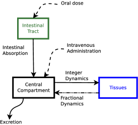
Amiodarone is an anti-arrhythmic agent which can be administered either intravenously (i.v.) or orally (Kühlkamp et al., 1999). It is well-known for its highly nonlinear non-exponential dynamics and singular long-term accumulation pattern. Dokoumetzidis et al. (2010) modeled the pharmacokinetic distribution of Amiodarone with a fractional compartmental model following a single intravenous and a single oral dose. The compartmental topology of the model is presented in Figure 1 where it is shown that the diffusion from the tissues to the central compartment is governed by a fractional-order dynamics.

Let $A_{1}$ and $A_{2}$ be the amounts of Amiodarone (in $\mathrm{ng}$) in the plasma and the tissues respectively and $u$ be the administration rate (in $\mathrm{ng}/\mathrm{day}$). We assume that the drug is administered directly into the central (plasma) compartment while the control objective is the concentration of the drug in the tissues attains a prescribed value (set-point). The fractional dynamical model we employ reads as follows:

$$\frac{\mathrm{d}A_{1}}{\mathrm{d}t} = -(k_{12}+k_{10})A_{1}+k_{21}\cdot\,{{}_{\mathrm{c}}\operatorname{D}}^{1-\alpha}A_{2}+u,$$ (1a)

$$\frac{\mathrm{d}A_{2}}{\mathrm{d}t} = k_{12}A_{1}-k_{21}\cdot\,{{}_{\mathrm{c}}\operatorname{D}}^{1-\alpha}A_{2},$$ (1b)

with $\alpha\in(0,1)$ and ${{}_{\mathrm{c}}\operatorname{D}}^{1-\alpha}$ is the Caputo fractional derivative which is defined in the following section.

2.2 Fractional-order derivatives

Several fractional-order derivatives have been proposed in the literature the most popular of which are the Riemann-Liouville ${{}_{\mathrm{rl}}\operatorname{D}}^{\alpha}$, the Caputo ${{}_{\mathrm{c}}\operatorname{D}}^{\alpha}$ and the Grünwald-Letnikov ${{}_{\mathrm{gl}}\operatorname{D}}^{\alpha}$ derivatives (Samko et al., 1993). These operators are used to formulate fractional-order differential equations, that is functional equations of the form

$$F(x(t),\operatorname{D}^{\alpha_{1}}x(t),\ldots,\operatorname{D}^{\alpha_{p}}x(t))=0,$$ (2)

where $\operatorname{D}^{\alpha}$ is a generalized derivative of order $\alpha\geq 0$. Typically, the Caputo derivative is used in this context as the initial conditions are easier to postulate.

The generalized Riemann-Liouville fractional-order integral operator of order $\alpha>0$ is given by

$$({{}_{\mathrm{rl}}\operatorname{I}}^{\alpha}f)(t)=\tfrac{1}{\Gamma(\alpha)}\int_{0}^{t}(t-\tau)^{\alpha-1}f(\tau)\mathrm{d}\tau,\ t\geq 0.$$ (3)

For $\alpha\in\mathbb{R}$ let us denote by $m=\lceil\alpha\rceil$ the smallest natural number $m$ so that $m\geq\alpha$. The following operator is known as the Caputo derivative of order $\alpha$:

$$({{}_{\mathrm{c}}\operatorname{D}}^{\alpha}f)(t)={{{}_{\mathrm{rl}}\operatorname{I}}}^{\,m-\alpha}\frac{\mathrm{d}^{m}f(t)}{\mathrm{d}t^{m}}.$$ (4)

The Grünwald-Letnikov fractional-order derivative is defined as

$$({{}_{\mathrm{gl}}\operatorname{D}}^{\alpha}f)(t)=\lim_{h\to 0}\tfrac{1}{h^{\alpha}}\sum_{i=0}^{\infty}(-1)^{i}\tbinom{\alpha}{i}f(t-ih),$$ (5)

where ${\alpha\choose 0}=1$ and $\binom{\alpha}{i}=\prod_{l=0}^{i-1}\tfrac{\alpha-l}{l+1}$.

The Laplace transform of the Caputo derivative of fractional order $\alpha\in(0,1)$ with zero initial conditions is given as $\mathcal{L}\left[({{}_{\mathrm{c}}\operatorname{D}}^{\alpha})(t)\right]=s^{\alpha}F(s)$, where $F(s)$ is the Laplace transform of function $f(t)$. The transfer function $G_{i}(s)=A_{i}(s)/U(s)$ which associates the administration rate $U(s)=\mathcal{L}u(t)$ to the concentrations $\hat{A}_{i}(s)=\mathcal{L}A_{i}(t)$ are:

$$G_{1}(s) =\frac{s^{\alpha}+k_{21}}{s^{\alpha+1}+k_{21}s+(k_{12}+k_{10})s^{\alpha}+k_{10}k_{21}},$$ (6a)

$$G_{2}(s) =\frac{k_{12}s^{\alpha-1}}{s^{\alpha+1}+k_{21}s+(k_{12}+k_{10})s^{\alpha}+k_{10}k_{21}},$$ (6b)

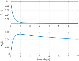
with $\alpha=0.587$, $k_{10}=1.4913\,\mathrm{day^{-1}}$, $k_{12}=2.9522\,\mathrm{day^{-1}}$ and $k_{21}=0.4854\,\mathrm{day^{-\alpha}}$. The concentration of Amiodarone in the two compartments with initial condition $A_{1}(0)=0.1\,\mathrm{ng}$ and $A_{2}(0)=0\,\mathrm{ng}$ is shown in Figure 2.

Figure 1: Strucutre of the fractional-order PK model of Amiodarone.

Figure 2: Open loop response of system (1) with initial conditions $A_{1}(0)=0.1\,\mathrm{ng},A_{2}(0)=0\,\mathrm{ng}$.

2.3 Solutions of FDEs

There can be identified four types of solutions for fractional-order differential equations: (i) analytical solutions, (ii) approximations in the $s$-domain using integer-order rational transfer functions and (iii) numerical approximation schemes in the discrete time domain, (iv) the numerical inverse Laplace transformation.

2.3.1 Analytical solutions.

Analytical solutions, when available, involve special functions such as the Mittag-Leffler function $\mathcal{E}_{\alpha,\beta}(t)=\sum_{k=0}^{\infty}{t^{k}}/{\Gamma(\alpha k+\beta)}$ whose evaluation requires in turn some numerical approximation scheme. Typically for the evaluation of the this function we resort to solving an FDE numerically (Garrappa, 2015a).

2.3.2 Transfer function approximations.

Rational approximations aim at approximating the transfer function of a fractional-order system — which involves terms of the form $s^{\alpha}$ — by ordinary transfer functions of the form

$$T(s)=\frac{P(s)}{Q(s)},$$ (7)

where $P$ and $Q$ are polynomials and the degree of $P$ is no larger than the degree of $Q$.

Padé Approximation: The Padé approximation of order $[m/n]$, $m,n\in\mathbb{N}$, at a point $s_{0}$ is rather popular and leads to rational functions with $\deg P=m$ and $\deg Q=n$ (Silva et al., 2006).

Matsuda-Fujii Method: This method consists in interpolating a function $H(s)$, which is treated as a black box, across a set of logarithmically spaced points (Matsuda and Fujii, 1993). By letting the selected points be $s_{k}$, $k=0,1,2,\dots$, the approximation is written as the continued fractions expansion

$$H(s)=\alpha_{0}+\frac{s-s_{0}}{\alpha_{1}+\frac{s-s_{1}}{\alpha_{2}+\frac{s-s_{2}}{\alpha_{3}+\dots}}}$$ (8)

where, $\alpha_{i}=\upsilon_{i}(s_{i})$, $\upsilon_{0}(s)=H(s)$, $\upsilon_{i+1}(s)=\frac{s-s_{i}}{\upsilon_{i}(s)-\alpha_{i}}$

Oustaloup’s method: Oustaloup’s method is based on the approximation of a function of the form:

$$H(s)=s^{\alpha},$$ (9)

with $\alpha>0$ by a rational function

$$\widehat{H}(s)=c_{0}\prod_{k=-N}^{N}\frac{s+\omega_{k}}{s+\omega^{\prime}_{k}}$$ (10)

within a range of frequencies from $\omega_{b}$ to $\omega_{h}$ (Oustaloup et al., 2000). The Oustaloup method offers an approximation at frequencies which are geometrically distributed about the characteristic frequency $\omega_{u}=\sqrt{\omega_{b}\omega_{h}}$ — the geometric mean of $\omega_{b}$ and $\omega_{h}$. The parameters $\omega_{k}$ and $\omega_{k}^{\prime}$ are determined via the design formulas (Petrás, 2011)

$$\omega_{k}^{\prime}=\omega_{b}\left(\frac{\omega_{h}}{\omega_{b}}\right)^{\frac{k+N+0.5(1+\alpha)}{2N+1}},$$ (11a)

$$\omega_{k}=\omega_{b}\left(\frac{\omega_{h}}{\omega_{b}}\right)^{\frac{k+N+0.5(1-\alpha)}{2N+1}},$$ (11b)

$$c_{0}=\left(\frac{\omega_{h}}{\omega_{b}}\right)^{-\frac{r}{2}}\prod_{k=-N}^{N}\frac{\omega_{k}}{\omega_{k}^{\prime}}.$$ (11c)

Parameters $\omega_{b}$, $\omega_{h}$ and $N$ are design parameters of the Oustaloup method.

Other methods: There are a few more methods which have been proposed in the literature to approximate fractional-order systems by rational transfer functions such as (Charef et al., 1992; Carlson and Halijak, 1964), as well as data-driven system identification techniques (Gao and Liao, 2012). Nice (Liang et al., 2014).

2.3.3 Time domain approximations.

Several methods have been proposed which attempt to approximate the solution to a fractional-order initial value problem in the time domain.

Grünwald-Letnikov: This is the method of choice in the discrete time domain where ${{{}_{\mathrm{gl}}\operatorname{D}}}^{\alpha}f$ is approximated by its discrete time variant

$$({{{}_{\mathrm{gl}}\Delta}}^{\alpha}x)_{k}=\tfrac{1}{h^{\alpha}}\sum_{i=0}^{\infty}(-1)^{i}\tbinom{\alpha}{i}x_{k-i},$$ (12)

which is in turn approximated by a discrete operator with finite memory $\nu$

$$({{{}_{\mathrm{gl}}\Delta}}^{\alpha}_{\nu}x)_{k}=\tfrac{1}{h^{\alpha}}\sum_{i=0}^{\nu}(-1)^{i}\tbinom{\alpha}{i}x_{k-i},$$ (13)

which is proven to have bounded error with respect to $({{{}_{\mathrm{gl}}\Delta}}^{\alpha}f)_{k}$ (Sopasakis and Sarimveis, 2017).

Numerical integration methods: Fractional-order initial value problems can be solved with various numerical methods such as the Adams-Bashforth-Moulton predictor-corrector (ABMPC) method (Zayernouri and Matzavinos, 2016) and fractional linear multi-step methods (FLMMs) (Garrappa, 2015b). These methods are only suitable for a system of FDE’s in the form

$${{}_{c}\operatorname{D}}^{\gamma}x(t) =f(t,x(t)),$$ (14a)

$$x^{(k)}(0) =x_{0,k},\,k=1,\dots,m-1$$ (14b)

where $\gamma$ is a rational, and $m=\lceil\gamma\rceil$.

In order to bring (1) in this form, we need to find a rational approximation of two derivatives, $1-\alpha$ and $1$. If we can find a satisfying rational approximation of $1-a\approxeq p/q$, then first order derivative follows trivially. Now, (1) can be written as

$${}_{c}\operatorname{D}^{\gamma}x_{0} =x_{1}$$ (15a)

$${}_{c}\operatorname{D}^{\gamma}x_{1} =x_{2}$$ (15b)

$$\ \,\vdots$$

$${}_{c}\operatorname{D}^{\gamma}x_{q-1} =-(k_{12}+k_{10})x_{0}{+}k_{21}x_{q+p}(t){+}u$$ (15c)

$${}_{c}\operatorname{D}^{\gamma}x_{q} =x_{q+1}(t)$$ (15d)

$$\ \,\vdots$$

$${}_{c}\operatorname{D}^{\gamma}x_{2q-1} =k_{12}x_{0}-k_{21}x_{q+p}$$ (15e)

subject to $x_{0}=A_{1}(0)$, $x_{q}=A_{2}(0)$ and $x_{i}(0)=0$ for $i\neq 1,q$, and $\gamma=1/q$. This system is in fact a linear fractional-order system for which analytical solutions are available (Kaczorek, 2011).

The number of states of system (15) is $2q$, therefore, the rational approximation should aim at a small $q$. In our case $1-\alpha=0.413$ can be written as $413/1000$, but then we would need to simulate a fractional-order system with $2000$ states. Instead $1-\alpha$ can be approximated by $19/46$ with error $0.413-19/46=-4.3478\cdot 10^{-5}$ or $216/523$ with error $0.413-216/523=-1.912\cdot 10^{-6}$. Such approximations can be obtained by means of continued fractions expansions of $1-\alpha$. Yet another reason to choose small $q$ is that small values of $\gamma=1/q$ render the system hard to simulate numerically.

Adams-Bashforth-Moulton predictor-corrector (ABMPC): Methods of the ABMPC type have been generalized to solve fractional-order systems. The basic concept is to evaluate $({{{}_{\mathrm{rl}}\operatorname{I}}}^{\gamma}f)(t,x(t))$ by approximating $f$ with appropriately selected polynomials. Solutions of (14) satisfy the following integral representation

$$x(t)=\sum_{k=0}^{m-1}x_{0,k}\frac{t^{k}}{k!}+({{{}_{\mathrm{rl}}\operatorname{I}}}^{\gamma}f)(t,x(t)),$$ (16)

where the first term on right hand side will be denoted with $T_{m-1}(t).$ The integral on the right hand side of the previous equation can be approximated, using an uniformly spaced grid $t_{n}=nh$, by $\frac{h^{\gamma}}{\gamma(\gamma+1)}\sum_{j=0}^{n+1}a_{j,n+1}f(t_{j})$ for suitable coefficients $a_{j,n+1}$ (Diethelm et al., 2002). The numerical approximation of the solution of (14) is

$$x(t_{n+1}) =T_{m-1}(t_{n+1})+\tfrac{h^{\gamma}}{\Gamma(\gamma+2)}f(t_{n+1},x_{p}(t_{n+1}))$$

$$+\sum_{j=1}^{n}a_{j,n+1}f(t_{j},x(t_{j})).$$ (17a)

The equation above is usually referred to as the corrector formula and $$x_{p}(t_{n+1})$$ is given by the predictor formula

$$x_{P}(t_{n+1})=T_{m-1}(t_{n}) +\tfrac{1}{\Gamma(\gamma)}\sum_{j=0}^{n}b_{j,n+1}f(t_{j},x(t_{j}).$$ (17b)

Unfortunately, the convergence error of ABMPC when $0<\gamma<1$ is $\mathcal{O}(h^{1+\gamma})$, therefore, a rather small step size $h$ is required to attain a reasonable aprpoximation error. A modification of the basic predictor-corrector method with more favorable computational cost is provided in (Garrappa, 2010) for which the MATLAB implementation fde12 is available.

Lubich’s method: Fractional linear multistep methods (FLMM) (Lubich, 1986) are a generalization of linear multistep methods (LMM) for ordinary differential equations. The key idea is to approximate the Riemann-Liouville fractional-order integral operator (3) with a discrete convolution, called convolution quadrature, as

$$({{}_{\mathrm{rl}}\operatorname{I}}_{h}^{\gamma}f)(t)\approxeq h^{\gamma}\sum_{j=0}^{n}\omega_{n-j}f(t_{j})+h^{\gamma}\sum_{j=0}^{s}w_{n,j}f(t_{j}),$$ (18)

for $t_{j}=jh,h>0$ where starting ($w_{n,j}$) and quadrature weights ($\omega_{n}$) are independent of $h$. Surprisingly, the latter weights can be constructed from any linear multistep method for arbitrary fractional order $\gamma$ (Lubich, 1986). Furthermore, FLMM constructed this way will inherit the same convergence rate and at least the same stability properties as the original LMM method (Lubich, 1985).

Here we use the MATLAB implementation flmm2 (Garrappa, 2015c) which is based on (Garrappa, 2015d). However, the method does not perform well for small $\gamma$. In our case study simulations we have found that values smaller than $0.1$ give poor results and often do not converge. However, when we used a more crude approximation of the original system with $\gamma=1/5$, flmm2 method was outperforming fde12 in terms of accuracy and has shown excellent stability properties with respect to bigger step size $h$.

2.3.4 Numerical inverse Laplace.

Several numerical inverse Laplace methods provide an approximation of

$$f(t)=\lim_{T\rightarrow\infty}\frac{1}{2\pi i}\int_{\sigma-iT}^{\sigma+iT}\e^{st}F(s)\d{s}.$$ (19)

for a given transfer function $F(s)$. Numerical methods can be used to directly evaluate the inversion integral (19) for non-rational transfer functions. One of the most popular methods is to convert the inversion integral into a Fourier transform and then approximate it by a Fourier series via trapezoid rule (de Hoog et al., 1982). These methods are considered to be precise for a broad class of function, but computationally demanding. An implementation of the above method is freely available on line (Hollenbeck, 1998).

A somewhat different approach is taken by Valsa and Brančik (1998), where authors approximate $\e^{st}$, the kernel of the inverse Laplace transformation, by $\tfrac{\e^{st}}{1+e^{-2a}e^{2st}}$ and choose $a$ appropriately so as to achieve an accurate inversion.

In general, numerical inversion methods can achieve high precision, but they are not suitable for control design purposes, especially for optimal control problems. Moreover, different methods are suited for various types of problems. An overview of the most popular inversion methods used in engineering practice is given in (Hassanzadeh and Pooladi-Darvish, 2007).

2.4 Assessment

In order to assess the accuracy of each approximation method presented above we introduce the following error indices

$$\|e_{i}\| =\sqrt{\int_{0}^{T_{s}}e_{i}(\tau)^{2}\mathrm{d}\tau},$$ (20)

$$\|e_{i}\|_{\infty} =\max_{t\in[0,T_{s}]}e_{i}(t),$$ (21)

where $T_{s}$ is a fixed simulation time and $e_{i}(t)$ is the difference between the approximate response of the system $\hat{A}_{i}$ and the one estimated by the inverse Laplace method of Valsa and Brančik (1998) with $a=11$ which is considered to be the most accurate.

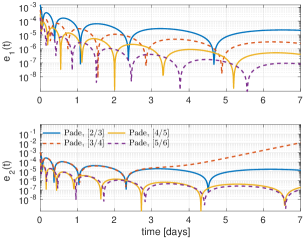
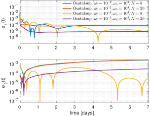
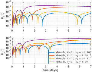
The pharmacokinetic profile following a single i.v. bolus dose is shown in Figure 2. In Figures 3, 4 and 5 we show the modeling errors $e_{i}(t)$ and in Tables 1, 2 and 3 we show the corresponding total errors. It seems that adequately high precision can be achieved with these methods. However, approximations in the $s$-domain are not suitable for constrained systems since there is no theoretical bound on the approximation error in the time domain.

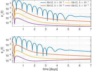
The errors of fde12 are presented in Figure 6 and Table 4. Using a step size as small as $h=10^{-5}$ fde12 achieves an approximation error which is uniformly lower than $10^{-4}$. In Figure 7 and Table 4 we show the approximation errors of the Grünwald-Letnikov method. It can be seen that the use of a long history is more important for the attainment of high precision compared to a small step size. Most likely as a result of the low value of $\gamma=0.0217$ in (15), flmm2 failed to produce reasonable approximations. We were in fact only able to produce moderately accurate approximations using $1-\alpha\approxeq 2/5$ where $\gamma=0.2$.

Figure 3: Absolute error of Padé approximation for various transfer function orders.

Figure 4: Absolute error of Oustaloup approximation for various parameters.

Figure 5: Absolute error of Matsuda-Fujii approximation for various parameters.

Table 1: Errors using the Padé approximation.

Order	$\|e_{1}\|$	$\|e_{2}\|$	$\|e_{1}\|_{\infty}$	$\|e_{2}\|_{\infty}$
$[2/3]$	$2.833\cdot 10^{-4}$	$1.907\cdot 10^{-4}$	$0.0015$	$0.001$
$[3/4]$	$1.105\cdot 10^{-4}$	$0.0059$	$6.094\cdot 10^{-4}$	$0.0113$
$[4/5]$	$4.514\cdot 10^{-5}$	$2.406\cdot 10^{-5}$	$3.076\cdot 10^{-4}$	$1.774\cdot 10^{-4}$
$[5/6]$	$2.327\cdot 10^{-5}$	$2.685\cdot 10^{-5}$	$1.752\cdot 10^{-4}$	$1.976\cdot 10^{-4}$

Table 2: Errors using the Oustaloup approximation.

$\omega_{b}$	$\omega_{h}$	$N$	$\|e_{1}\|$	$\|e_{2}\|$	$\|e_{1}\|_{\infty}$	$\|e_{2}\|_{\infty}$
$10^{-2}$	$10^{3}$	$8$	$0.0023$	$0.0043$	$0.0228$	$0.0025$
$10^{-2}$	$10^{4}$	$20$	$5.744\cdot 10^{-4}$	$0.0045$	$0.0054$	$0.0027$
$10^{-3}$	$10^{3}$	$8$	$0.0033$	$5.084\cdot 10^{-4}$	$0.0332$	$6.555\cdot 10^{-4}$
$10^{-3}$	$10^{4}$	$20$	$7.451\cdot 10^{-4}$	$4.597\cdot 10^{-4}$	$0.0074$	$2.765\cdot 10^{-4}$

Table 3: Errors using the Matsuda-Fujii approximation with $s_{k}=\beta^{\alpha_{k}}$.

$\beta$	$\alpha_{k}$	$\|e_{1}\|$	$\|e_{2}\|$	$\|e_{1}\|_{\infty}$	$\|e_{2}\|_{\infty}$
$2$	$-1:10$	$7.01\cdot 10^{-5}$	$3.162\cdot 10^{-4}$	$4.82\cdot 10^{-5}$	$2.111\cdot 10^{-4}$
$2$	$1:10$	$0.0016$	$0.0036$	$0.0009$	$0.0032$
$2.3$	$-1:11$	$0.0002$	$0.0032$	$0.0018$	$0.003$
$3$	$1:10$	$0.0034$	$0.0127$	$0.0017$	$0.0075$

Figure 6: Absolute error of fractional differential equation solution by means of fde12 method where fractional order $1-a=0.413$ is approximated by $19/46$.

Figure 7: Absolute error of GL method for various step sizes and history lengths.

Table 4: Approximation errors of fde12

$h$	$\|e_{1}\|$	$\|e_{2}\|$	$\|e_{1}\|_{\infty}$	$\|e_{2}\|_{\infty}$
$10^{-2}$	$0.0333$	$0.0223$	$0.0584$	$0.0368$
$10^{-3}$	$0.0020$	$0.0013$	$0.0083$	$0.0055$
$10^{-4}$	$1.782\cdot 10^{-4}$	$1.157\cdot 10^{-4}$	$7.982\cdot 10^{-4}$	$5.204\cdot 10^{-4}$
$10^{-5}$	$1.669\cdot 10^{-5}$	$1.113\cdot 10^{-5}$	$7.412\cdot 10^{-4}$	$4.824\cdot 10^{-4}$

Table 5: Approximation errors of the Grünwald-Letnikov method

$h$	$h\nu$	$\|e_{1}\|$	$\|e_{2}\|$	$\|e_{1}\|_{\infty}$	$\|e_{2}\|_{\infty}$
$10^{-2}$	$3$	$8.165\cdot 10^{-4}$	$0.0022$	$8.223\cdot 10^{-4}$	$0.0021$
$10^{-2}$	$5$	$5.302\cdot 10^{-4}$	$4.571\cdot 10^{-4}$	$8.223\cdot 10^{-4}$	$5.911\cdot 10^{-4}$
$10^{-2}$	$7$	$5.126\cdot 10^{-4}$	$3.640\cdot 10^{-4}$	$8.223\cdot 10^{-4}$	$5.911\cdot 10^{-4}$
$10^{-3}$	$3$	$6.390\cdot 10^{-4}$	$0.0022$	$4.735\cdot 10^{-4}$	$0.0021$
$10^{-3}$	$5$	$1.454\cdot 10^{-4}$	$2.760\cdot 10^{-4}$	$1.727\cdot 10^{-4}$	$4.057\cdot 10^{-4}$
$10^{-3}$	$7$	$5.060\cdot 10^{-5}$	$3.594\cdot 10^{-5}$	$8.067\cdot 10^{-4}$	$5.797\cdot 10^{-4}$

3 Administration scheduling

In this section we address the problem of administration scheduling. Our objective is to devise an administration schedule — a sequence of dosages — so that the concentration of Amiodarone in the tissues is close to a desired value, while the concentration in both compartments never exceeds certain safety limits. We also have to account for a limit on allowed drug dose at each time instant. In doing so, we must assume that we are not able to measure drug concentrations during the treatment. All of these requirements and constraints can be elegantly integrated within the framework of constrained optimal control.

3.1 Optimal control

In this section we describe the optimal control problem formulation. We start by discretizing (1) with a sampling time $t_{c}$ yielding

$$t_{c}^{-1}(x_{k+1}-x_{k})=Ax_{k}+F{{}_{\mathrm{gl}}\Delta}^{1-a}_{\nu}x_{k}+Bu_{k}$$ (22)

where $x_{k}=\left[A_{1}(kt_{c})\,\,A_{2}(kt_{c})\right]^{\prime}$. The left hand side of (22) corresponds to the forward Euler approximation of the first-order derivative, and we shall refer to $t_{c}=10^{-2}\,\mathrm{days}$ as the control sampling time. Matrices $A,F$ and $B$ are

$$A=\begin{bmatrix}-(k_{12}+k_{10})&0\\ k_{21}&0\\ \end{bmatrix},F=\begin{bmatrix}0&k_{21}\\ 0&-k_{21}\\ \end{bmatrix},B=\begin{bmatrix}1\\ 0\\ \end{bmatrix}.$$ (23)

The discrete-time dynamic equations of the system can now be stated as

$$x_{k+1}=x_{k}+t_{c}\bigg{(}Ax_{k}+\frac{F}{t_{c}^{1-a}}\sum_{j=0}^{\nu}c_{j}^{1-a}x_{k-j}+Bu_{k}\bigg{)},$$ (24)

where $c_{j}^{\alpha}=(-1)^{j}\binom{\alpha}{j}$. By augmenting the system with past values as $\tilde{x}_{k}=(x_{k},x_{k-1},\dots,x_{k-\nu+1})$ we can rewrite (24) as a finite-dimension linear system

$$\tilde{x}_{k+1}=\hat{A}\tilde{x}_{k}+\hat{B}u_{k}.$$ (25)

Matrices $\hat{A}$ and $\hat{B}$ are straightforward to derive and are given in (Sopasakis and Sarimveis, 2017). The therapeutic session will last for $N_{d}=Nt_{c}=7\,\mathrm{days}$ in total, where $N$ is called the prediction horizon. It is not realistic to administer the drug to the patient too frequently, so we assume that the patient is to receive their treatment every $t_{d}=0.5\,\mathrm{days}$. The administration schedule must ensure that the concentration of drug in all compartments never exceeds the minimum toxic concentration limits while tracking the prescribed reference value as close as possible. To this aim we postulate the following constrained optimal control problem.

$$\min_{\{u_{0},\ldots,u_{N_{d}-1}\}}J =\sum_{k=0}^{N_{d}/t_{c}+1}(x_{\mathrm{ref},k}-x_{k})^{\prime}Q(x_{\mathrm{ref},k}-x_{k})$$ (26a)

subject to

$$\tilde{x}_{k+1} =\hat{A}\tilde{x}_{k}+\hat{B}u_{j},\text{ for }\ kt_{c}=jt_{d}$$ (26b)

$$\tilde{x}_{k+1} =\hat{A}\tilde{x}_{k},\text{ otherwise}$$ (26c)

$$0 \leq x_{k}\leq 0.5$$ (26d)

$$0 \leq u_{j}\leq 0.5$$ (26e)

for $$k=0,\ldots,N j=0,\ldots,N_{d}-1$$; .

In the above formulation $x_{\mathrm{ref},k}$ is the desired drug concentration at time $k$ and operator ^′ denotes vector transposition. Any deviation from set point is penalized by weight matrix $Q=\mathrm{diag}([0\;1])$. Note that we are tracking only the second state. Our underlying GL model has a relative history of $t_{c}\nu=5\,\mathrm{days}$. Optimal drug concentrations are denoted by $u^{\star}_{k}$, for $k=0,\dots,N_{d}-1$ and they correspond to dosages administered intravenously at times $kt_{d}$. In the optimal control formulation we have implicitly assumed that $t_{d}$ is an integer multiple of $t_{c}$, which is not restrictive since $t_{c}$ can be chosen arbitrarily. Finally, we can recognize that problem (26) is a standard quadratic problem that can be readily solved. In our simulations, we have used YALMIP (Löfberg, 2004) to model the problem and MOSEK (ApS, 2015) as the underlying solver to calculate the solution.

3.2 Simulations

To argue for the soundness and the applicability of our approach in real-world scenarios, we will apply the optimal drug dosage schedule to a more precise model than (25). For this purpose we will use fde12 solver. As evident from the results in the previous section, for sufficiently small solver time $h_{sol}$, we can have a realistic simulation of the system.

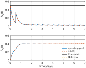
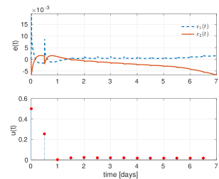
After solving the optimal control problem we applied the optimal sequence to the FDE simulator fde12. Results are shown in Figures 8 and 9. It can be seen that open loop predictions of the GL model and fde12 simulation show high agreement. This should not be surprising considering that all of the parameters describing the patient are nominal and, additionally, shows that the GL model is of good quality.

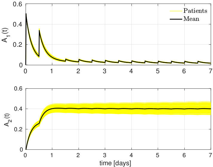
Next, we consider multiple patients that are characterized by perturbed parameters. We will simulate the behaviour of $100$ different patients with multiplicative perturbations on parameters $k_{10},k_{12}$ and $k_{21}$. Each parameter is multiplied by a constant drawn from a uniform distribution on the interval $\left[0.85,1.15\right]$. Moreover, the order of the fractional derivative $\alpha=1-\hat{p}/q$ is given by a random choice of $\hat{p}$ from a set of discrete values $\{17,18,20,21\}$, each one having the same probability. Denominator $q$ is fixed at $q=46$, while the nominal numerator is $p=19$. We simulate each patient by applying the same optimal drug scheduling sequence that was computed for the nominal one, that is, without online information about the state of each patient. Results are shown in Figure 10.

Figure 8: Open loop control of drug administration with a fixed scheduling. Step size for fde12 was set to $h=10^{-5}$.

Figure 9: (Up) errors of predicted states via GL model against fde12. (Down) optimal administration sequence.

Figure 10: Fixed schedule drug administration for a population of $100$ patients. Step size for fde12 was set to $h=10^{-5}$.

4 Conclusions

This paper gives an overview of the state of the art in numerical methods for the simulation of fractional-order systems along with validation results on a fractional-order pharmacokinetic model taken from the literature. Results are shown regarding the solution of an open-loop optimal control problem for the administration of Amiodarone to a patient whose pharmacokinetic parameters are assumed to be perfectly known. Additionally, we presented optimal control results for different patients whose pharmacokinetic parameters are not know perfectly. This way, we estimate and demonstrate how sensitive the administration scheduling is.

References

- ApS (2015) MOSEK ApS. The MOSEK optimization toolbox for MATLAB manual. Version 7.1 (Revision 28)., 2015. URL http://docs.mosek.com/7.1/toolbox/index.html.
- Carlson and Halijak (1964) G. Carlson and C. Halijak. Approximation of fractional capacitors by a regular Newton process. IEEE Transactions on Circuit Theory, 11(2):210–213, Jun 1964.
- Charef et al. (1992) A. Charef, H. H. Sun, Y. Y. Tsao, and B. Onaral. Fractal system as represented by singularity function. IEEE Transactions on Automatic Control, 37(9):1465–1470, Sep 1992.
- de Hoog et al. (1982) F.R. de Hoog, J.H. Knight, and A.N. Stokes. An improved method for numerical inversion of laplace transforms. SIAM Journal on Scientific and Statistical Computing, 3:357, 1982.
- Diethelm et al. (2002) K. Diethelm, N. J. Ford, and A. D. Freed. A predictor-corrector approach for the numerical solution of fractional differential equations. Nonlinear Dynamics, 29(1):3–22, 2002.
- Dokoumetzidis and Macheras (2008) A. Dokoumetzidis and P. Macheras. IVIVC of controlled release formulations: Physiological-dynamical reasons for their failure. Journal of Controlled Release, 129(2):76–78, 2008.
- Dokoumetzidis and Macheras (2011) A. Dokoumetzidis and P. Macheras. The changing face of the rate concept in biopharmaceutical sciences: From classical to fractal and finally to fractional. Pharmaceutical Research, 28(5):1229–1232, 2011.
- Dokoumetzidis et al. (2010) A. Dokoumetzidis, R. Magin, and P. Macheras. Fractional kinetics in multi-compartmental systems. Journal of Pharmacokinetics and Pharmacodynamics, 37(5):507–524, 2010.
- Gao and Liao (2012) Z. Gao and X. Liao. Rational approximation for fractional-order system by particle swarm optimization. Nonlinear Dynamics, 67(2):1387–1395, 2012.
- Garrappa (2010) R. Garrappa. On linear stability of predictor-corrector algorithms for fractional differential equations. Int. J. Comput. Math., 87(10):2281–2290, 2010.
- Garrappa (2015a) R. Garrappa. Numerical evaluation of two and three parameter Mittag-Leffler functions. SIAM J. Numerical Analysis, 53:1350–1369, 2015a.
- Garrappa (2015b) R. Garrappa. Trapezoidal methods for fractional differential equations: Theoretical and computational aspects. Mathematics and Computers in Simulation, 110:96 – 112, 2015b. 7th edition of the workshop “Structural Dynamical Systems: computational aspects”.
- Garrappa (2015c) R. Garrappa. Fractional software. https://www.dm.uniba.it/Members/garrappa/Software, 2015c. Accessed: 2016-11-04.
- Garrappa (2015d) R. Garrappa. Trapezoidal methods for fractional differential equations: Theoretical and computational aspects. Mathematics and Computers in Simulation, 110:96–112, 2015d.
- Hassanzadeh and Pooladi-Darvish (2007) H. Hassanzadeh and M. Pooladi-Darvish. Comparison of different numerical laplace inversion methods for engineering applications. Applied Mathematics and Computation, 189(2):1966 – 1981, 2007. ISSN 0096-3003.
- Hollenbeck (1998) K. J. Hollenbeck. Invlap.m: A matlab function for numerical inversion of laplace transforms by the de hoog algorithm. http://www.mathworks.com/matlabcentral/answers/uploaded_files/1034/invlap.m, 1998. Accessed: 2016-11-04.
- Kaczorek (2011) T. Kaczorek. Selected Problems of Fractional Systems Theory. Springer Berlin Heidelberg, 2011. 10.1007/978-3-642-20502-6. URL http://dx.doi.org/10.1007/978-3-642-20502-6.
- Kühlkamp et al. (1999) V. Kühlkamp, C. Mewis, R. Suchalla, J. Mermi, V. Dörnberger, and L. Seipel. Effect of amiodarone and sotalol on the defibrillation threshold in comparison to patients without antiarrhythmic drug treatment. International Journal of Cardiology, 69(3):271–279, 1999.
- Liang et al. (2014) S. Liang, C. Peng, Z. Liao, and Y. Wang. State space approximation for general fractional order dynamic systems. International Journal of Systems Science, 45(10):2203–2212, 2014.
- Löfberg (2004) J. Löfberg. Yalmip : A toolbox for modeling and optimization in MATLAB. In Proceedings of the CACSD Conference, Taipei, Taiwan, 2004. URL http://users.isy.liu.se/johanl/yalmip.
- Lubich (1985) C. Lubich. Fractional linear multistep methods for abel-volterra integral equations of the second kind. Mathematics of Computation, 45(172):463–469, 1985.
- Lubich (1986) C. Lubich. Discretized fractional calculus. SIAM J. Math. Anal., 17(3):704–719, 1986.
- Matsuda and Fujii (1993) K. Matsuda and H. Fujii. H(infinity) optimized wave-absorbing control - analytical and experimental results. Journal of Guidance, Control, and Dynamics, 16(6):1146–1153, nov 1993.
- Oustaloup et al. (2000) A. Oustaloup, F. Levron, B. Mathieu, and F. M. Nanot. Frequency-band complex noninteger differentiator: characterization and synthesis. IEEE Transactions on Circuits and Systems I: Fundamental Theory and Applications, 47(1):25–39, Jan 2000.
- Petrás (2011) I. Petrás. Fractional Derivatives, Fractional Integrals, and Fractional Differential Equations in Matlab. InTech, oct 2011.
- Samko et al. (1993) S. Samko, A. Kilbas, and O. Marichev. Fractional integral and derivatives. Gordon & Breach Science Publishers, 1993.
- Silva et al. (2006) M.F. Silva, J.A.T. Machado, and R.S. Barbosa. Comparison of different orders padé fractional order pd0.5 control algorithm implementations. IFAC Proceedings Volumes, 39(11):373 – 378, 2006.
- Sopasakis and Sarimveis (2017) P. Sopasakis and H. Sarimveis. Stabilising model predictive control for discrete-time fractional-order systems. Automatica, 75:24–31, January 2017.
- Sopasakis et al. (2015) P. Sopasakis, S. Ntouskas, and H. Sarimveis. Robust model predictive control for discrete-time fractional-order systems. In Control and Automation (MED), 2015 23th Mediterranean Conference on, pages 384–389, June 2015.
- Valsa and Brančik (1998) J. Valsa and L. Brančik. Approximate formulae for numerical inversion of laplace transforms. International Journal of Numerical Modelling: Electronic Networks, Devices and Fields, 11(3):153–166, 1998.
- Zayernouri and Matzavinos (2016) M. Zayernouri and A. Matzavinos. Fractional adams–bashforth/moulton methods: An application to the fractional keller–segel chemotaxis system. Journal of Computational Physics, 317:1 – 14, 2016.