Astrophysical properties of star clusters in the Magellanic Clouds homogeneously estimated by ASteCA

Abstract

Aims. To produce an homogeneous catalog of astrophysical parameters of 239 resolved star clusters located in the Small and Large Magellanic Clouds, observed in the Washington photometric system.

Methods. The cluster sample was processed with the recently introduced Automated Stellar Cluster Analysis (ASteCA) package, which ensures both an automatized and a fully reproducible treatment, together with a statistically based analysis of their fundamental parameters and associated uncertainties. The fundamental parameters determined with this tool for each cluster, via a color-magnitude diagram (CMD) analysis, are: metallicity, age, reddening, distance modulus, and total mass.

Results. We generated an homogeneous catalog of structural and fundamental parameters for the studied cluster sample, and performed a detailed internal error analysis along with a thorough comparison with values taken from twenty-six published articles. We studied the distribution of cluster fundamental parameters in both Clouds, and obtained their age-metallicity relationships.

Conclusions. The ASteCA package can be applied to an unsupervised determination of fundamental cluster parameters; a task of increasing relevance as more data becomes available through upcoming surveys.

1 Introduction

The study of a galaxy’s structure, dynamics, star formation history, chemical enrichment history, etc., can be conducted from the analysis of its star clusters. Star clusters in the Magellanic Clouds (MCs) are made up of a varying number of coeval stars sharing a chemical composition, assumed to be located relatively at the same distance from the Sun, and affected by roughly the same amount of reddening. These factors facilitate the estimation of their fundamental parameters, and thus the properties of their host galaxy. New developments in astrophysical software allow the homogeneous processing of different types of star clusters’ databases. The article series by Kharchenko et al. (see Kharchenko et al., 2005; Schmeja et al., 2014, and references therein) and the integrated photometry based derivation of age and mass for 920 clusters presented in Popescu et al. (2012), based on their MASSsive CLuster Evolution and ANalysis package (MASSCLEAN, Popescu & Hanson, 2009), are examples of semi-automated and automated packages applied on a large number of clusters.

However, there is no guarantee that by employing a homogeneous method, we will obtain similar parameter values from the same cluster photometric data set across different studies. This is particularly true when the methods require user intervention, which makes the results subjective to some degree. In Netopil et al. (2015) the open cluster parameters age, reddening, and distance are contrasted throughout seven published databases. The authors found that all articles show non-negligible offsets in their fundamental parameter values. This result highlights an important issue: most of the color-magnitude diagram (CMD) isochrone fits are done by-eye, adjusting correlated parameters independently, and often omitting a proper error treatment (see von Hippel et al., 2014, for a more detailed description of this problem). When statistical methods are employed, the used code is seldom publicly shared to allow scrutiny by the community. There is then no objective way to asses the underlying reliability of each set of results. Lacking this basic audit, the decision of which database values to use becomes a matter of preference.

As demonstrated by Hills et al. (2015), assigning precise fundamental parameters for an observed star cluster is not a straightforward task. Using combinations of up to eight filters ($UBVRIJHK_{s}$) and three stellar evolutionary models, they analyzed the NGC188 open cluster with a Bayesian isochrone fitting technique implemented in their BASE-9 package, and arrived at statistically different results depending on the isochrones and the filters used. NGC188 is a ${\sim}4$ Gyr cluster with a well defined Main Sequence (MS) mostly unaffected by field star contamination, and with proper motions and radial velocities data available. A typical situation – where a star cluster is observed through fewer filters, affected by a non-negligible amount of field star contamination, and without information about its dynamics – will be significantly more complicated to analyze. A mismatch between theoretical evolutionary models, along with an inability to reproduce clusters in the unevolved MS domain, had already been reported in Grocholski & Sarajedini (2003).

The aforementioned difficulties in the analysis of star cluster CMDs will only increase if the study is done by-eye, since: a) the number of possible solutions manually fitted is several orders of magnitude smaller than that handled by a code, b) correlations between parameters are almost entirely disregarded, c) uncertainties can not be assigned through valid mathematical means – and are often not assigned at all –, and d) the final values are necessarily highly subjective. In the last thirty years, many authors have applied some form of statistical analysis to derive star clusters’ fundamental parameters. We give in Sect 2.9 of Perren et al. (2015, hereafter Paper I) a non-exhaustive list of articles where these methods were employed. Still, by-eye studies continue to be used. This is because most statistical methods developed are either closed-source, or restricted to a particular form of analysis (or both). The need is clear for an automated general method with a fully open and extensible code base, that takes as much information into account as possible, and capable of generating reliable results.

In Paper I we presented the Automated STEllar Cluster Analysis (ASteCA) package, aimed at allowing an accurate and comprehensive study of star clusters. The code is released under a GPL v3 general public license, and can be downloaded from its official site. Through a mostly unassisted process the code analyses clusters’ positional and photometric data sets to derive their fundamental parameters and uncertainties. As shown in Paper I, the code is able to assign precise parameter values for clusters with low to medium field star contamination, and gives reasonable estimations for heavily contaminated clusters. Every part of this astrophysical package is open and publicly available, and its development is ongoing.

In the present work we apply ASteCA on 239 clusters in the Small and Large Magellanic Clouds (S/LMC), distributed up to ${\sim}5^{\circ}$ and ${\sim}8^{\circ}$ in angular distance from their centers, respectively. The MCs are located close enough to us to allow the study of their resolved star clusters. The large number of cataloged clusters – $\sim 4000$ are listed in the Bica et al. (2008) catalog – makes them an invaluable resource for investigating the properties of the two most massive galaxies that orbit the Milky Way. The reddening that affects the MCs is relatively small, except for a few regions like 30 Doradus in the LMC, where $E_{B-V}$ can reach values above $0.4$ mag (Piatti et al., 2015a). The overall low levels of reddening simplifies the research of the clusters in these two galaxies. We use photometric data sets in the $CT_{1}$ the Washington system (Canterna, 1976; Geisler, 1996), known to be highly sensitive to metal abundance for star clusters older than ${\sim}1$ Gyr (Geisler & Sarajedini, 1999). The results obtained here regarding the metal content, are thus of relevance for the analysis of the MCs chemical enrichment history.

This is the first study where such a large sample of resolved star clusters is homogeneously analyzed in an automatic way, with their fundamental parameters statistically estimated rather than fitted by eye or fixed a priori. Having metal content assigned for 100% of our sample is particularly important, especially compared to other star cluster catalogs. The latest version of the well known DAML02 database (v3.5, 2016 Jan 28; Dias et al., 2002), for example, reports abundances for only 13% out of the 2167 clusters cataloged. Estimations for the total cluster mass is given in few cases, if integrated photometry is provided.

This article is structured as follows. In Sect. 2 we present the star cluster sample used in this work along with numerous studies used to compare and validate our results. Sections 3 and 4 describe the estimation of the fundamental parameters derived with ASteCA, and analyze their uncertainties, respectively. In Sect. 5 a detailed comparison of our results with published values from the literature is performed. Sect. 6 shows the distribution of cluster fundamental parameters in our catalog, and the age-metallicity relationships (AMRs) for the cluster system. Sect. 7 summarizes our results and concluding remarks.

2 Clusters sample

The data set used in this work consists of $CT_{1}$ Washington photometry for 239 star clusters; 150 of them located in the LMC and the rest in the SMC. These clusters were selected because they were readily available, are already analyzed in the literature – meaning we can compare the published parameters with the estimates produced in this work –, and are sufficiently dispersed throughout both galaxies. In Fig. 1 we show their spatial distribution.

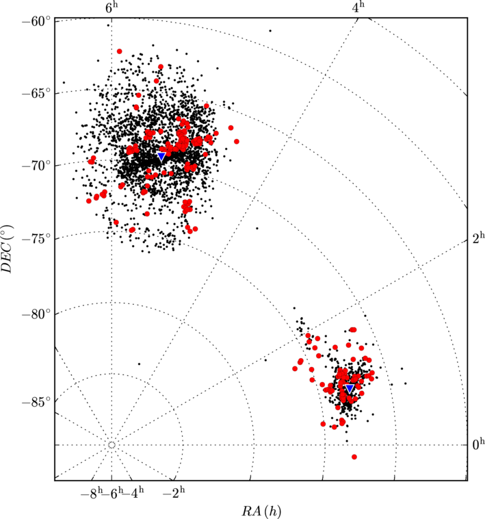
Figure 1: Distribution of our set of analyzed clusters (red circles) superimposed on to the Bica et al. (2008) database of 3740 star clusters (black dots), for both MCs. The assumed centers for the Clouds are marked with blue triangles.

Table 1 lists the nineteen articles that analyzed the same $CT_{1}$ photometry used by ASteCA in the current study. Hereafter, we will refer to this group as the “literature”. Metallicities, ages, reddenings, and distance moduli ($\mu_{\circ}$) were estimated or assigned in the literature, except for the 36 clusters in Piatti (2011b) which had only their ages estimated via the $\delta T_{1}$ index (Phelps et al., 1994; Geisler et al., 1997). In most of the literature metallicities and the distance moduli are fixed to $[Fe/H]{=}-0.7$ dex, $[Fe/H]{=}-0.4$ dex, and $\mu_{\circ}{=}18.9$ mag and $\mu_{\circ}{=}18.5$ mag, for the S/LMC respectively. Ages reported in the literature were obtained by eye matching, either through the standard isochrone technique or applying the $\delta T_{1}$ index method. Reddenings were estimated in almost all cases interpolating the maps of either Burstein & Heiles (1982), Schlegel et al. (1998), or Haschke et al. (2011). Maia et al. (2013) presented total mass estimations for their 29 star clusters sample.

Our cluster sample was also partially studied via Johnson-Kron-Cousins photometry, as listed in Table 2. This group will be referred as the “databases” (DBs), as a way to distinguish them from the “literature”. In Sect. 5 we compare the parameter values obtained by ASteCA, to those given in both the literature and the databases.

Table 1: Sources of the $CT_{1}$ data sets used in this work. $N$ refers to the number of clusters analyzed per article.

Article	$N$	Galaxy	Telescope
Geisler et al. (2003)	8	LMC	CTIO 0.9m
Piatti et al. (2003b)	5	LMC	CTIO 0.9m
Piatti et al. (2003a)	6	LMC	CTIO 0.9m
Piatti et al. (2005)	8	SMC	CTIO 0.9m
Piatti et al. (2007a)	4	SMC	CTIO 0.9m
Piatti et al. (2007c)	2	SMC	Danish 1.54m
Piatti et al. (2007b)	2	SMC	Danish 1.54m
Piatti et al. (2008)	6	SMC	Danish 1.54m
Piatti et al. (2009)	5	LMC	CTIO 0.9m / Danish 1.54m
Piatti et al. (2011b)	3	LMC	CTIO 0.9m
Piatti et al. (2011a)	14	SMC	CTIO 1.5m
Piatti (2011a)	9	SMC	Blanco 4m
Piatti (2011b)	36	LMC	Blanco 4m
Piatti (2011c)	11	SMC	Blanco 4m
Piatti (2012)	26	LMC	Blanco 4m
Piatti & Bica (2012)	4	SMC	Blanco 4m
Palma et al. (2013)	23	LMC	Blanco 4m
Maia et al. (2013)	29	SMC	Blanco 4m
Choudhury et al. (2015)	38	LMC	Blanco 4m

Table 2: Sources of Johnson-Kron-Cousins photometric data sets for some clusters in our sample. $N$ refers to the number of clusters in common with our sample per article.

Article	$N$	Galaxy	Phot
Pietrzynski & Udalski (1999), P99	7	SMC	$BVI$
Pietrzynski & Udalski (2000), P00	25	LMC	$BVI$
Hunter et al. (2003), H03	62	S/LMC	$UBVR$
Rafelski & Zaritsky (2005), R05	24	SMC	$UBVI$
Chiosi et al. (2006), C06	16	SMC	$VI$
Glatt et al. (2010), G10	61	S/LMC	$UBVI$
Popescu et al. (2012), P12	48	LMC	$UBVR$

3 Estimation of star cluster parameters

Fundamental – metallicity, age, distance modulus, reddening, mass – and structural – center coordinates, radius, contamination index, approximate number of members, membership probabilities, true cluster probability – parameters, were obtained either automatically or semi-automatically with ASteCA. A detailed description of the functions built within this tool can be found in Paper I, and in the code’s online documentation. The resulting catalog can be accessed via VizieR. We have made available the Python codebase developed to analyze the data obtained with ASteCA, and generate the figures in this article. Output images generated by ASteCA for each cluster, can be accessed through a separate public code repository.

3.1 Ranges for fitted fundamental parameters

To processes a cluster, the user must provide ASteCA a suitable range of accessible values for each fundamental parameter by setting a minimum, a maximum, and a step. As explained in Sect. 3.4, each combination of values from the five fundamental parameters represents a unique synthetic CMD, or model. The larger the number of accessible parameter values, the larger the amount of models the code will process to find the synthetic CMD which best matches the observed cluster CMD. Ranges and steps were selected to provide a balance between a large interval, and a computationally manageable number of total models; see Table 3. Special care was taken to avoid defining ranges that could bias the results towards a particular region of any fitted parameter.

Unlike most previous works where the metallicity is a fixed value, we do not make assumptions on the cluster’s metal content. Our [Fe/H] interval covers completely the usual metallicities reported for MCs’ clusters. The age range encompasses almost the entire allowed range of the CMD service where the theoretical isochrones were obtained from (see Sect. 3.4).

The maximum allowed value for the reddening of each cluster was determined through the Magellanic Clouds Extinction Values (MCEV) reddening maps (Haschke et al., 2011), while the minimum value is always zero. We used TOPCAT to query $E_{V-I}$ values from these maps, within a region as small as possible around the position of each cluster. For 85% of our sample we found several regions with associated reddening values, within a box of 0.5 deg centered on the cluster’s position. For the remaining clusters, larger boxes had to be used. The two most extreme cases are NGC1997 ($\alpha{=}5^{h}30^{m}34^{s}$, $\delta{=}-63^{\circ}12^{\prime}12^{\prime\prime}$ [J2000.0]) and OHSC28 ($\alpha{=}5^{h}55^{m}35^{s}$, $\delta{=}-62^{\circ}20^{\prime}43^{\prime\prime}$ [J2000.0]) in the outers of the LMC, where boxes of 4 deg and 6 deg respectively where needed to find a region with assigned reddening values. In both cases, the reddenings given by the Schlafly & Finkbeiner (2011) map for their coordinates are up to two times smaller than the ones found in the MCEV map. We adopted the largest $E_{V-I}$ value of each region, MCEV_max, as the upper limit in the reddening range. Three steps are used to ensure that the reddening range is partitioned similarly for all MCEV_max values: 0.01 for MCEV${}_{\max}{>}0.1$, 0.02 if $0.05{\leq}\mathrm{MCEV}_{\max}{\leq}0.1$, and 0.005 for MCEV${}_{\max}{<}0.05$. The $E_{V-I}$ extinction is converted to $E_{B-V}$ following Tammann et al. (2003): $E_{V-I}{=}1.38\,E_{B-V}$. An extinction law of $R_{v}{=}3.1$ is applied throughout the analysis.

Mean distance moduli for the S/LMC Clouds were taken from de Grijs & Bono (2015) and de Grijs et al. (2014). Line of sight (LOS) depths for the MCs (front to back, $\pm 1\sigma$) have been reported to span up to 20 kpc in their deepest regions (Subramanian & Subramaniam, 2009; Nidever et al., 2013; Scowcroft et al., 2015). The 0.1 mag deviations allowed in this work give LOS depths of ${\sim}5.7$ kpc and ${\sim}4.6$ kpc for the S/LMC. This covers more than half of the average LOS depths found in Subramanian & Subramaniam (2009) for the SMC (bar: $4.9\pm 1.2$ kpc, disk: $4.23\pm 1.48$ kpc), and the LMC (bar: $4.0\pm 1.4$ kpc, disk: $3.44\pm 1.16$ kpc). Although this is not enough to cover the entire observed depth ranges, it gives the distance moduli liberty to move around their mean values when all parameters are adjusted.

The maximum total cluster mass was set to $10000\,M_{\odot}$. To estimate this value, a first rough pass was performed with ASteCA for all clusters in our dataset. Most of them were assigned total masses below $5000\,M_{\odot}$, making the $10000\,M_{\odot}$ limit a reasonable value. This was true for all except 15 visibly massive clusters, for which the maximum mass was increased to $30000\,M_{\odot}$. We will see in Sect 5.2.1 that the code is systematically underestimating masses, due to the stellar crowding effect on our set of Washington photometry.

Binary fraction was fixed to 0.5 – considered a reasonable estimate for clusters (von Hippel, 2005; Sollima et al., 2010) – to avoid introducing an extra degree of complexity into the fitting process. Secondary masses are randomly drawn from a uniform mass ratio distribution of the form $0.7{\leq}q{\leq}1$, where $q{=}M_{2}/M_{1}$, and $M_{1}$, $M_{2}$ are the primary and secondary masses. This range for the secondary masses was found for the LMC cluster NGC1818 in Elson et al. (1998), and represents a value commonly used in analysis regarding the MCs (see Rubele et al., 2011, and references therein).

Table 3: Fundamental parameters’ ranges used by ASteCA on our set of 239 clusters. The approximate number of values used for each parameter is $N$. This gives a combined total of ${\sim}2.3{\times}10^{7}$ possible models (or synthetic cluster CMDs), that could be theoretically matched to each studied cluster in our sample.

Parameter	Min	Max	Step	$N$
[Fe/H]	$\sim$-2.2	0	$\sim$0.1	23
$\log\mathrm{(age/yr)}$	6.	10.1	0.05	82
$E_{B-V}$	0.0	MCEVmax	${\sim}$0.01	$\sim$12
$\mu_{SMC}$	18.86	19.06	0.02	10
$\mu_{LMC}$	18.4	18.6	0.02	10
Mass ($M_{\odot}$)	10	[1, 3]${\times}10^{4}$	200	[50, 150]

3.2 Center and radius assignment

ASteCA employs a two-dimensional Gaussian kernel density estimator (KDE) to determine the center of the cluster. A radial density profile (RDP) is used to estimate the cluster’s radius, as the point where the RDP reaches the surrounding field’s mean density.

The density of cluster members must make it stand out over the combination of foreground/background stars, with no other over-density present in the observed frame (this limitation is planned to be lifted in upcoming versions of ASteCA). A portion of the surrounding field should be visible, and the RDP must be reasonably smooth. When these conditions are not met, the semi-automatic mode can be used. Here center coordinates are either obtained based on an initial set of approximate values, or manually fixed along with the radius value.

For ${\sim}66\%$ of our sample, center coordinates were obtained via a KDE analysis, based on initial approximate values. Radii were calculated for ${\sim}60\%$ of the clusters, through an RDP analysis of their surrounding fields. The remaining clusters are those that are highly contaminated, contain very few observed stars, and/or occupy most of the observed frames. This means that an estimation of their centers and/or radii was not possible, and their values were manually fixed.

The contamination index ($CI$) is a parameter related to the number of foreground/background stars in the cluster region. See Paper I, Sect. 2.3.2 for a complete mathematical definition of the index. Values of $0,\,0.5$, and $\,{>}0.5$ mean respectively: the cluster is not contaminated by field stars, an equal number of field stars and cluster members are present in the cluster region, more field stars are expected within the cluster region than cluster stars. For reference, the average $CI$ for the set of clusters with manual radii assignment is $CI{\simeq}0.9{\pm}0.2$, and $CI{\simeq}0.6\pm 0.2$ for those clusters whose radii were estimated in automatic mode.

3.3 Field-star decontamination

A decontamination algorithm (DA) was employed on the $CT_{1}$ CMD of each processed cluster to remove field-star contamination. The Bayesian DA presented in Paper I was improved for the present analysis; the new DA works in two steps. First, the original Bayesian membership probability (MP) assignation is applied to the CMD of all stars within the cluster region (see Paper I for more details). After that the CMD is binned into cells, and a cleaning algorithm is used to remove stars of low MPs cell-by-cell as shown in Fig. 2. By default ASteCA uses the Bayesian blocks method introduced in Scargle et al. (2013), via the implementation of the astroML package (Vanderplas et al., 2012). While Bayesian blocks binning is the default setting in ASteCA, several others techniques for CMD star removal are available, as well as five more binning methods. This second step is similar to the DA developed in Bonatto & Bica (2007, B07), which uses a simpler rectangular grid. The main difference, aside from the binning method employed, is that ASteCA removes stars based on their MPs, not randomly as done in B07.

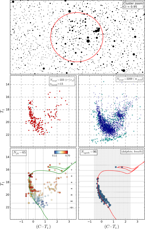
Figure 2: Top: SMC-L62 cluster and surrounding field stars region. The adopted radius is marked with a red circle. The CI value in the top right box is the “contamination index”, see Sect. 3.2. Middle: CMD of the cluster region for SMC-L62 (left), where $n_{memb}$ is the approximate number of cluster stars. The CMD of ten combined surrounding field regions, each with an area equal to that of the cluster, is also shown (right). In both panels $N_{accpt}$ is the number of stars that were not rejected due to their large photometric errors. Rejected stars with large errors are shown as pale green crosses. Bottom: cluster region after applying the DA (left); MPs vary according to the colorbar at the top right. Dotted horizontal and vertical lines show the binning used to reject low MP stars cell-by-cell, as obtained via the Bayesian blocks method. Open circles (drawn semi-transparent) represent rejected stars. $N_{fit}$ is the number of stars kept unsubtracted by the cell-by-cell rejection. The best fitted isochrone is overplotted with a green line. The respective generated synthetic CMD is shown in the right panel. $N_{synth}$ is the number of stars in the synthetic cluster CMD, and the dotted lines represent the binning obtained using Knuth’s rule, applied in the synthetic cluster match process. The limiting magnitude of the synthetic CMD is taken from the limiting magnitude of the observed cluster (roughly $T_{1}{\approx}22$ mag, in this case).

Approximately 70% of our sample was processed with these default settings. The remaining ${\sim}$30%, those with a low number of cluster stars or heavily contaminated, were processed with modified settings to allow a proper field-star decontamination. Changes introduced were, for instance, a different binning method (often a rectangular grid using Scott’s rule, Scott, 1979), or skipping the Bayesian MP assignation and only performing a density based cell-by-cell field star removal. In this latter case, the DA works very similarly to the B07 algorithm.

An appropriate field-star decontamination is of the utmost importance, since the cleaned cluster CMDs will be used to estimate the cluster fundamental parameters.

3.4 Synthetic CMD matching

ASteCA derives clusters’ fundamental parameters matching their observed CMDs with synthetic CMDs. In this work these are built using PARSEC v1.1 theoretical isochrones (Bressan et al., 2012, B12), and a log-normal initial mass function (IMF, Chabrier, 2001). For a given age, metallicity, total mass, and binary fraction, a synthetic CMD is built from a stochastically sampled IMF down to the faintest portion of the theoretical isochrone (defined by the metallicity and age values), shifted by a reddening and distance modulus. For a detailed description on the generation of synthetic CMDs from theoretical isochrones by ASteCA, see: Paper I, Sect. 2.9.1. All the evolutionary tracks from the CMD service are currently supported, as well as three other IMFs.

The Poisson likelihood rate (PLR, Dolphin, 2002) is employed to asses the match between the cluster’s CMD and a synthetic CMD, out of the ${\sim}2{\times}10^{7}$ possible solutions (as shown in Table 3). The PLR statistic requires binning the cluster’s CMD, and the synthetic CMDs generated according to the fundamental parameter ranges defined in Sect.3.1. We use Knuth’s rule (Knuth, 2006, also implemented via the astroML package) as the default binning method (see bottom right plot in Fig. 2). The inverted logarithmic form of the PLR can be written as

$$LPLR=-2\ln PLR=2\sum_{i}m_{i}-n_{i}+n_{i}\ln\frac{n_{i}}{m_{i}},$$ (1)

where $m_{i}$ and $n_{i}$ are the number of stars in the $i$th cell (two-dimensional bin) of the synthetic and the observed cluster’s CMD, respectively. If for any given cell we have $n_{i}\neq 0$ and $m_{i}=0$, a very small number is used instead ($m_{i}=1{\times}10^{-10}$) to avoid a mathematical inconsistency with the factor $\ln m_{i}$. Although ASteCA does not currently provide a goodness-of-fit estimator, uncertainties associated to the fitted fundamental parameters can be though of as a coarse measure of the fit’s robustness. This parameter is to be added in upcoming versions of the code.

In Paper I the total mass parameter could not be estimated, due to the likelihood statistic used (Paper I, Eq. 11). The LPR defined in Eq. 1 allows us to also consider the mass as a free parameter in the search for the best synthetic CMD. The total mass is estimated simultaneously along with the remaining fundamental parameters of a cluster, no extra process is employed (for example, a mass-luminosity relation). Following the validation performed in Paper I for the metallicity, age, reddening, and distance, we present in Appendix A a similar study for the total mass. We demonstrate that the masses recovered by ASteCA for nearly 800 MASSCLEAN synthetic clusters – with masses ranging from 500 $M_{\odot}$ to $2.5\times 10^{5}\,M_{\odot}$ – are in excellent agreement with the masses used to generate them.

The determination of any fundamental parameter depends exclusively on the distribution and number of observed stars in the cluster’s CMD. Since we deal with five free fundamental parameters, a 5-dimensional surface of solutions is built from all the possible synthetic CMDs. ASteCA applies a genetic algorithm (GA) on this surface to derive the cluster’s fundamental parameters. After the GA returns the optimal fundamental parameter values, uncertainties are estimated via a standard bootstrap technique. This process takes a significant amount of time to complete, since it involves running the GA several more times on a randomly generated cluster with replacement. Generating a new cluster “with replacement”, means randomly picking stars one by one from the original cluster, where any star can be selected more than once. The process stops when the same number of stars as those present in the original cluster have been picked. We run the bootstrap ten times per cluster, as it would be prohibitively costly timewise to run it – as would be ideal – hundreds or even thousands of times. On average, the CMD of each cluster in our dataset was compared t ${\sim}1{\times}10^{6}$ synthetic CMDs, once the full process was completed.

4 Errors in fitted parameters

It is well known that a parameter given with no error estimation is meaningless from a physical standpoint (Dolphin, 2002; Andrae, 2010). Despite this, a detailed error treatment is often ignored in articles that deal with star clusters analysis (Paunzen & Netopil, 2006).

As explained in Sect. 3.4, ASteCA employs a bootstrap method to assign standard deviations for each fitted parameter. The code simultaneously fits five free parameters within a wide range of allowed values, using only a 2-dimensional space of observed data, i.e., the $T_{1}$ versus $(C-T_{1})$ CMD; meaning uncertainties will be somewhat large. We plan to upgrade the code to eventually allow more than just two observed magnitudes, extending the 2-dimensional CMD analysis to an N-dimensional one. It is worth noting that, unlike manually set errors, these are statistically valid uncertainty estimates. This is an important point to make given that the usual by-eye isochrone fitting method not only disregards known correlations among all clusters parameters, it is also fundamentally incapable of producing a valid error analysis (Naylor & Jeffries, 2006). Any uncertainty estimate produced by-eye serves only as a mere approximation, which will often be biased towards smaller figures. The average logarithmic age error given in the literature, for example, is 0.16 dex, in contrast with the almost twice as large average value estimated by ASteCA (see below). In Fig. 3 we show the distribution of standard deviations of the five fundamental parameters fitted by the code, for the entire sample.

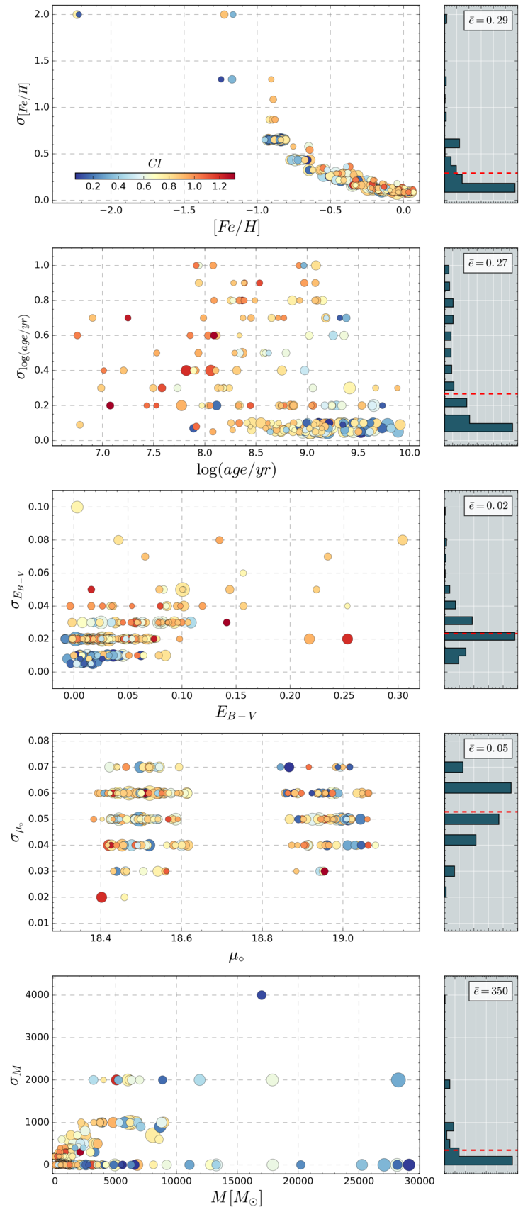
Figure 3: Left: Distribution of errors versus the five parameters fitted by ASteCA. Colors are associated to the $CI$ (see bar in top plot), sizes are proportional to the actual cluster sizes. A small random scatter in the x-axis is added for clarity. Right: Error histogram. The mean error value for each parameter is shown in the top right corner, and drawn in the plot with a dashed red line.

The apparent dependence of the metallicity error with decreasing [Fe/H] values arises from the fact that ASteCA uses $z$ values, where $\mathrm{[Fe/H]}{=}\log(z/z_{\odot})$; with $z_{\odot}{=}0.0152$. We use $z$ instead of [Fe/H] because: a- this is the default form in which the evolutionary tracks are generated by the CMD service, and b- it is easier to work with the code when all parameters are strictly positive. The error in $z$ is $\sigma_{z}{\approx}0.003$ for over 75% of the clusters analyzed. This means that, when converting to $e_{[Fe/H]}$ using the relation

$$\sigma_{[Fe/H]}=\sigma_{z}/[z\times\ln(10)],$$ (2)

the $z$ in the denominator makes $\sigma_{[Fe/H]}$ grow as it decreases, while $\sigma_{z}$ remains approximately constant. For very small $z$ values (e.g.: $z{=}0.0001$), the logarithmic errors can surpass $\sigma_{[Fe/H]}{=}2$ dex. In those cases the error is trimmed to 2 dex, enough to cover the entire metallicity range.

There are no visible error trends for any of the fitted parameters, a desirable feature for any statistical method. If a parameter’s uncertainty varied (increase/decrease) with it, it would indicate ASteCA was introducing biases in the solutions.

Histograms to the right of Fig. 3 show the distribution of errors, and their arithmetic means as a dashed red line. For $\sim$34% and ${\sim}69\%$ of the S/LMC clusters we have $\sigma_{[Fe/H]}{<}0.2$ dex. Approximately 53% of the combined S/LMC sample show $\sigma_{\log(age/yr)}{<}0.1$ dex. Error estimates for the remaining parameters are all within acceptable ranges. The uncertainties tend to increase for clusters of lower mass, due to the inherent stochasticity of the fitting process.

Errors could be lowered applying different techniques: increase the number of models evaluated in the GA, reduce the value of the steps in the parameters’ range, or increase the number of bootstrap runs. These methods, particularly the latter, will extend the time needed to process each cluster. Limited computational time available requires a balance between the maximum processing power allocated to the calculations, and the aimed precision. Error values presented here should then be considered a conservative upper limit.

5 Comparision with published fundamental parameters

We compare in Sect. 5.1 the parameter values obtained by ASteCA, with those taken from the papers that used the same $CT_{1}$ data sets (see Table 1), referred as the “literature”. The parameters age, reddening, and mass are also analyzed in Sect 5.2 for a subset of 142 star clusters that could be cross-matched with $UBVRI$ photometry results (see Table 2), referred as the “databases”.

5.1 Literature values

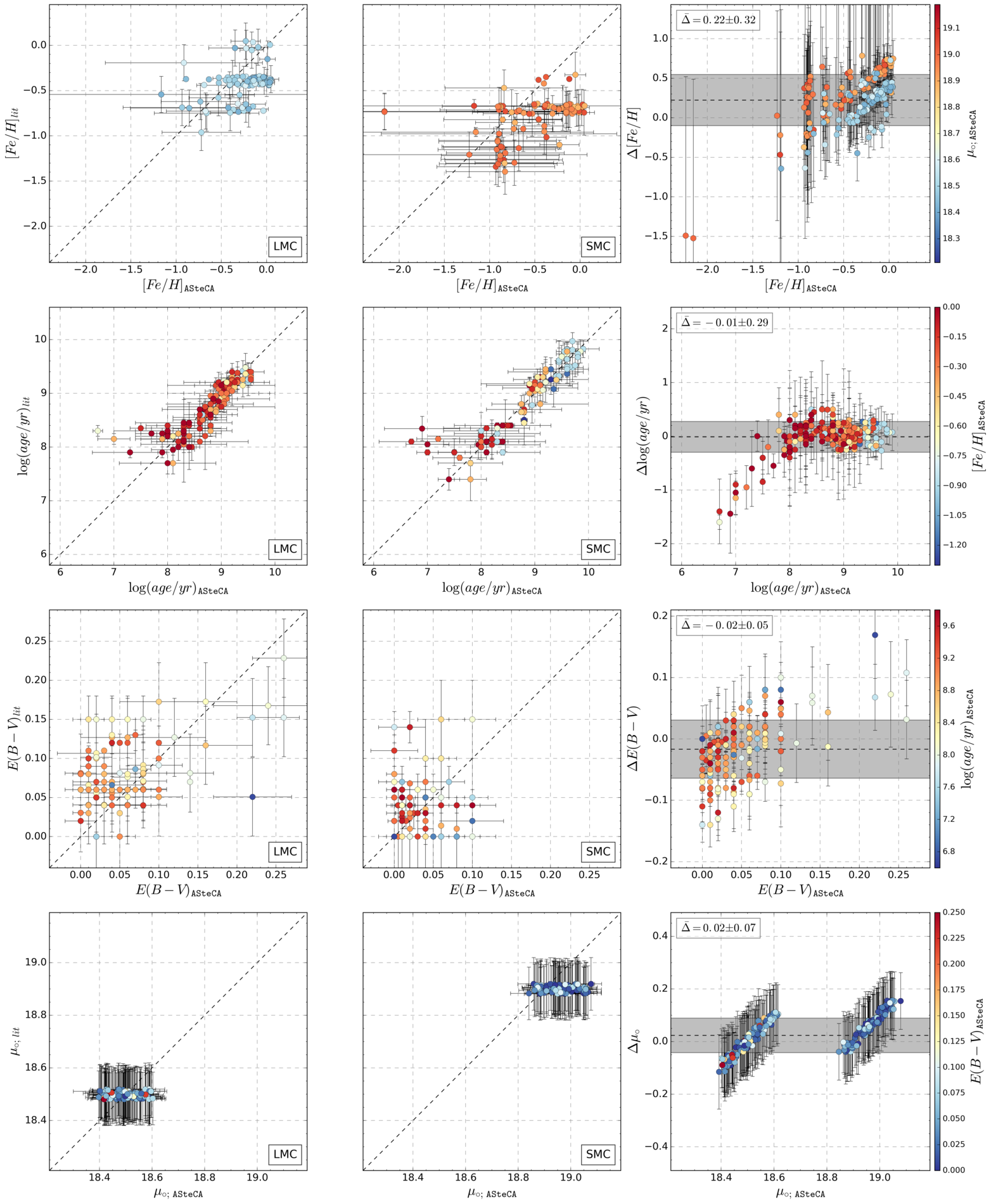
Figure 4: Left column: parameters comparison for the LMC. Center column: idem for the SMC. Right column: BA plot with differences in the sense $\Delta$= (ASteCA minus literature), for the combined S/LMC sample. A small random scatter is added to both axes for the metallicity and distance modulus plots. Mean and standard deviation of the differences, $\overline{\Delta}$, are shown as a dashed line and a gray band, respectively; their values are displayed in the top left of the plot. Colors follow the bar at the right of the figure, for each row. Piatti (2011b) clusters with age information only are plotted with $E_{B-V}{=}0$.

ASteCA versus literature values for the metallicity, age, reddening, and distance modulus, are presented in Fig. 4. Left and central panels show the 1:1 identity line for both galaxies. Right panel diagram shows a Bland-Altman (BA) plot for our combined sample of clusters, with the variation in the x-axis proposed by Krouwer (Bland & Altman, 1986; Krouwer, 2008). The BA is also called a “difference” or “Tukey Mean-Difference” plot. In the original BA plot the default x-axis displays the mean values between the two methods being compared. The Krouwer variation changes the means for the values of one of those methods, called the “reference”. In our case, the reference is ASteCA so we use its reported values in the x-axis.

ASteCA abundance estimates are slightly larger than those in the literature, seen as offsets in the upper panels of Fig. 4. On average, the offset is $\sim$0.27 dex and $\sim$0.18 dex for the S/LMC. This effect can be explained by two different processes, in light of our knowledge that the ASteCA’s best fit CMD matching introduces no biases into the solutions. First, ASteCA’s $z$ values are converted to the logarithmic form [Fe/H] using a solar metallicity of $z_{\odot}{=}0.0152$ (Bressan et al., 2012). Literature values, on the other hand, are converted using a solar metal content of $z_{\odot}{=}0.019$ (Marigo et al., 2008) (usually rounded to 0.02). This means that ASteCA will give [Fe/H] values larger by ${\sim}0.1$ dex, for any fitted isochrone of equivalent $z$ being compared, following

$$\begin{split}\Delta\mathrm{[Fe/H]}&=\mathrm{[Fe/H]}_{\mathtt{ASteCA}}-\mathrm{[Fe/H]}_{literature}\\ &=\log(z/0.0152)-\log(z/0.019)=\log(0.019/0.0152)\\ &\approx 0.0969\;\mathrm{dex}\end{split}$$ (3)

Second, the MC’s star clusters are often studied using fixed metallicities. For example, [Fe/H] values assumed in the 19 literature articles, are exactly -0.7 dex and -0.4 dex for $\sim$60% and $\sim$75% of S/LMC clusters. The by-eye fit is biased towards the assignment of these particular abundances, due to the effect of “confirmation bias”. This effect present in the published literature has been studied recently by de Grijs et al. (2014), in relation to distance measurement reported for the LMC. Alternatively, the code is left free to fit metal contents in the entire range given. The [Fe/H] values estimated by ASteCA are distributed mainly between -1 dex and 0 dex, but clustered closer to solar metal content than to lower metallicities. This fact, combined with the above mentioned effect of mostly fixed [Fe/H] values used in the literature, makes the averaged difference in assigned metal content be slightly positive. It also is responsible for the apparent linear growth of $\Delta$[Fe/H] as $\mathrm{[Fe/H]}_{\mathtt{ASteCA}}$ increases, seen in Fig. 4. Researchers tend to fit isochrones adjusting it to the lower envelope of a cluster’s sequence. This is done to avoid the influence of the binary sequence (located above and to the right of the single stars sequence in a CMD) in the fit, but it can also contribute to the selection of isochrones of smaller metallicity. The reason is that increasing an isochrone’s metal content moves it towards redder (greater color) values in a CMD, see for example Bressan et al. (2012), Fig 15. These combined effects explain the offset found for the abundances. It is important to notice that neither effect is intrinsic to the best likelihood matching method used by the code.

The general dispersion between literature and ASteCA values can be quantized by the standard deviation of the $\Delta$ differences in the BA plot. This value is $\sim$0.32 dex for the metallicity, in close agreement with the mean internal [Fe/H] uncertainty found in Sect. 4. ASteCA’s mean metallicities for the MCs are $\mathrm{[Fe/H]}_{SMC}{\simeq-}0.52{\pm}0.44$ dex, and $\mathrm{[Fe/H]}_{LMC}{\simeq-}0.26{\pm}0.24$ dex. These averages are similar, within their uncertainties, to those obtained using literature values: $\mathrm{[Fe/H]}_{SMC}{\simeq-}0.78{\pm}0.23$ dex, and $\mathrm{[Fe/H]}_{LMC}{\simeq-}0.42{\pm}0.16$ dex

Ages show an overall good agreement, with larger differences seen for a handful of young clusters. Ten clusters with either a shallow photometry, a low number of cluster stars, or heavily contaminated, present age differences larger than $\Delta\log(age/yr){>}0.5$ dex. These are referred to as “outliers”, and discussed in more depth in Appendix B. The mean $\Delta\log(age/yr)$ value for all S/LMC clusters, -0.01 dex as shown in the age BA plot of Fig. 4, points to an excellent agreement in $\log(age/yr)$. Excluding outliers, this mean increases to $\sim$0.04 dex.

Similarly to what was found for the metallicity, the $\sim$0.3 dex dispersion is almost exactly the internal uncertainty found for errors assigned by the code.

The reddening distribution presents maximum $E_{B-V}$ values of $\sim$0.15 mag and $\sim$0.3 mag for the S/LMC, respectively. The $\Delta$ differences are well balanced with a standard deviation of 0.05 mag, slightly larger than the 0.02 mag average uncertainty found for internal errors. We estimate average $E_{B-V}$ values for the S/LMC of $0.03{\pm}0.03$ mag and $0.05{\pm}0.05$ mag. These estimates are approximately a third of those used for example in the Hunter et al. (2003) study, because our sample does no contain clusters in the regions of the MCs most affected by dust.

Distance moduli ($\mu_{\circ}$) found by ASteCA show a clear displacement from literature values. This is expected, as the clusters’ distance in the literature articles is always assumed equivalent to the distance to the center of the corresponding galaxy. The distribution of $\mu_{\circ}$ values found by the code covers the entire range allowed in Sect. 3.1. It is worth noting that this variation appears to have no substantial effect on any of the remaining parameters, something that could in principle be expected due to the known correlations between them (see Paper I, Sect. 3.1.4). This reinforces the idea that using a fixed value for the distance modulus, as done in the literature, is a valid way of reducing the number of free variables at no apparent extra cost.

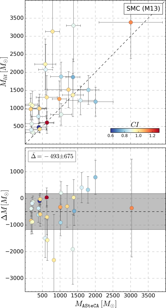
Figure 5: Top: Mass comparison for ASteCA versus literature values. Bottom: BA plot with mean and standard deviation of the differences shown as a dashed horizontal line, and a gray band respectively. The mean and standard deviation values are displayed in the top left corner.

Masses are only assigned in Maia et al. (2013, M13) for its sample of 29 SMC clusters. The comparison with ASteCA is presented in Fig. 5, where the top panel shows a trend for ASteCA masses to be smaller than those from M13. This is particularly true for the clusters with the largest mass estimates – and the largest assigned errors – in M13: H86-97 (3300$\pm$1300$M_{\odot}$), and H86-87 (3100$\pm$1700$M_{\odot}$). The BA plot (bottom) shows that, on average, M13 masses are ${\sim}500{\pm}700\,M_{\odot}$ larger. To explain these differences, we need to compare the way total cluster masses are obtained by M13 and ASteCA.

ASteCA estimates masses matching synthetic CMDs to that of the observed cluster region. The radius that delimits this region is formally equivalent to the tidal radius defined in (King, 1962, see Sect. 3.2), but it is in practice smaller due to observational effects (i.e, Poisson errors in star counts, photometric incompleteness, field stars contamination). A fraction of cluster members is thus left out of the analysis when this radius is used. We can prove using King’s derivation of the number of members for a cluster (Eq. 18, King, 1962), that this fraction is small except for highly underestimated radii ($r{<}0.5r_{t}$) and very low concentration clusters ($r_{t}/r_{c}{<}2$). Massive clusters are largely unaffected by this process, while uncertainties for low-mass clusters’ masses are large enough that this effect can be safely ignored. To err on the side of caution, ASteCA masses should be considered lower estimates of the true present-day cluster masses.

In M13 cluster masses were determined using two methods, based on estimating a mass function via the $T_{1}$ luminosity function (LF). In both cases a field star cleaning process was applied. The first one employs a CMD decontamination procedure (Maia et al., 2010), and the second one cleans the cluster region’s LF by subtracting it a field star LF. Results obtained with these two methods are averaged to generate the final mass values. Although any reasonable field star cleaning algorithm should remove many or most of the foreground/background stars in a cluster region, some field stars are bound to remain. For heavily contaminated clusters this effect will be determinant in shaping the “cleaned” CMD sequence, as cluster stars will be very difficult to disentangle from contaminating field stars. Clusters in M13 are indeed heavily affected by field star contamination, as seen in Fig. 5 where colors follow their $CI$s. The minimum value is $CI{\simeq}0.55$, meaning all cluster regions are expected to contain, on average, more field stars than cluster stars. A large number of contaminating field stars not only makes the job much harder for the DA, it also implies that the LF will most likely be overestimated. This leads – in the case of M13 – to an overestimation of the total mass. In contrast, ASteCA assigns masses taking their values directly from the best match synthetic CMD. Field star contamination will thus have a lower influence on the code’s mass estimate, limited just to how effective the DA is in cleaning the cluster region. We find in Appendix A that the code will slightly underestimate masses by approximately 200 $M_{\odot}$, for low mass clusters. This is unrelated to the fraction of members lost due to the employed radius (mentioned previously), since we use in this analysis the full tidal radius to delimit the MASSCLEAN synthetic clusters region. These combined effects explain the ${\sim}500\,M_{\odot}$ offset found for mass values, seen in Fig. 5.

The case of B48 is worth mentioning, as it is the cluster with the largest total mass given in M13 (3400$\pm$1600$M_{\odot}$). After removing possible field stars – see Sect. 3.3 – low mass stars disappear, and B48 is left only with its upper sequence ($T_{1}<18.4$ mag). This happens both in M13, see Fig. C8, and the ASteCA analysis, see left CMD in Fig. 6. The likelihood (Eq. 1) sees then no statistical benefit in matching the cluster’s CMD with a synthetic CMD of similar age and mass, which will contain a large number of low mass stars. This leads the GA to select synthetic CMDs of considerably younger ages ($\log(age/yr){<}7.0$ dex) than that assigned in M13 ($\log(age/yr){=}7.9\pm 0.05$ dex), and with much lower mass estimates (see caption of Fig. 6). Age and mass values similar to those from M13 could be found by the code, only if the DA was applied with no cell-by-cell removal of low MP stars as shown in the right CMD of Fig. 6. This means that all field stars within the cluster region are used in the synthetic CMD matching process, which inevitably questions the reliability of the total mass estimate. Dealing with this statistical effect is not straightforward and will probably require an extra layer of modeling added to the synthetic CMD generation algorithm. As discussed in Appendix B this effect also plays an important role in the significant age differences found between ASteCA and the literature, for a handful of outliers.

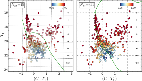
Figure 6: Left: Best fit isochrone for B48 found by ASteCA when a cell-by-cell removal is applied, following the Bayesian MP assignation (removed stars are drawn semi-transparent). Estimated age and total mass are $\log(age/yr){=}6.2{\pm}0.6$, and $M{=}400{\pm}200\,M_{\odot}$. Right: Best fit isochrone found when no removal of stars is performed, and the full cluster region is used in the search for the best synthetic cluster match. Estimated age and total mass are now $\log(age/yr){=}7.5{\pm}0.3$, and $M{=}3000{\pm}900\,M_{\odot}$.

5.2 Databases values

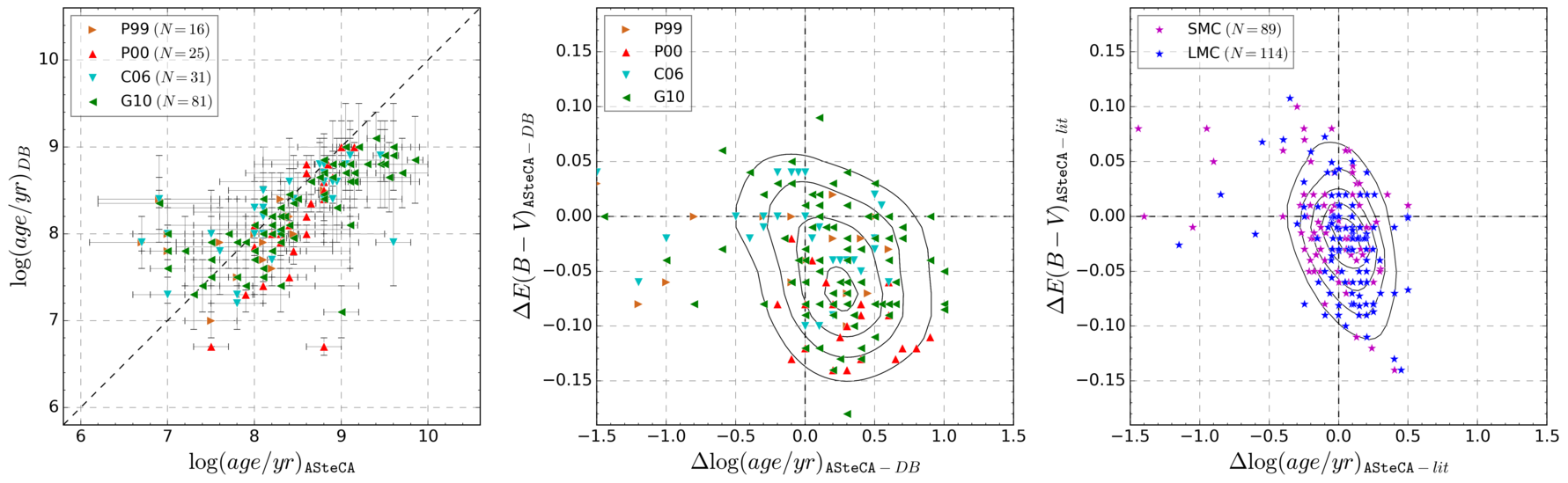
Figure 7: Left: age comparison for DBs that used the isochrone fit method versus ASteCA, where $N$ is the number of clusters cross-matched in each DB. Center: “delta” plot (ASteCA minus DB) showing differences between reddening and age. Curves represent regions of iso-densities after fitting a 2-dimensional Gaussian Kernel. Right: same as previous plot, for ASteCA minus literature values for both Clouds.

We compare our results with those from seven articles – the “databases” or DBs – where a different photometric system was used; see Table 2. These DBs are separated into two groups: those where the standard by-eye isochrone fitting method was applied – P99, P00, C06, and G10 – and those where integrated photometry was employed – H03, R05, and P12. A total of 142 clusters from our sample could be cross-matched. Where names were not available to perform the cross-match – P00, P99, and R05 – we employed a 20 arcsec finding radius, centered on the equatorial coordinates of the clusters.

ASteCA versus the four isochrone-fit DBs ages, are shown in Fig. 7, left and center plot. P99 and P00 analyze SMC and LMC clusters respectively, using Bertelli et al. (1994) isochrones and fixed S/LMC metallicities $z{=}0.004,0.008$. While P99 derives individual reddening estimates based on red clump stars, P00 uses reddening values determined for 84 lines-of-sight in the Udalski et al. (1999) LMC Cepheids study. Both studies attempt to eliminate field star contamination following the statistical procedure presented in Mateo & Hodge (1986). These DBs employed distance moduli of 18.65 mag and 18.24 mag for the S/LMC, approximately ${\sim}0.25$ mag smaller than the canonical distances assumed for each Cloud. This has a direct impact on their obtained ages. In de Grijs & Anders (2006) the authors estimate that had P00 used a value of $\mu_{0}{=}18.5$ mag instead, their ages would be ${\sim}0.2{-}0.4$ dex younger; the same reasoning can be applied to the P99 age estimates. A similar conclusion is reached by Baumgardt et al. (2013). Notice that in the latter the authors correct the age bias that arises in P00 due to the small distance modulus used, increasing P00 age estimates by 0.2 dex. This is incorrect, ages should have been decreased by that amount. P99 and P00 logarithmic ages are displaced on average from ASteCA values (in the sense ASteCA minus DB) by $-0.13{\pm}0.6$ dex and $0.37{\pm}0.5$ dex respectively, as seen in Fig. 7 left plot. In the case of P99, the distance modulus correction would bring the age values to an overall agreement with ASteCA, although with a large scatter around the identity line. P00 age values on the other hand, would end up ${\sim}0.7$ dex below the code’s age estimates after such a correction. Such a large deviation is most likely due to the overestimated reddening values used by P00, as will be shown below.

C06 studied 311 SMC clusters via isochrone fitting applying two methods: visual inspection and a Monte Carlo based $\chi^{2}$ minimization. The authors also employ a decontamination algorithm, making this the article that more closely resembles our work. Distance modulus is fixed to $\mu_{0}{=}18.9$ mag, reddening and metallicity values of $E_{B-V}{=}0.08$ mag and $z{=}0.008$ are used, adjusted when necessary to improve the fit. It is worth noting that the [Fe/H]${=}-0.4$ dex abundance employed in C06 is closer to the [Fe/H]${=}-0.52{\pm}0.44$ dex ASteCA average for the SMC, than the canonical [Fe/H]${=}-0.7$ dex value used in most works. Out of the seven DBs, C06 is the one that best matches ASteCA’s $\log(age/yr)$ values, with a mean deviation from the identity line of $0.02\pm 0.58$ dex.

G10 analyzed over 1500 clusters with ages ${<}1$ Gyr in both Clouds via by-eye isochrone fitting. They assumed distance moduli of (18.9, 18.5) mag, and metallicities of (0.004, 0.008), for the S/LMC respectively. Reddening was adjusted also by-eye on a case-by-case basis. This DB presents a systematic bias where smaller logarithmic ages are assigned compared to our values, with an approximate deviation of $\Delta\log(age/yr){\simeq}0.23\pm 0.46$ (ASteCA minus G10). This is consistent with the results found in Choudhury et al. (2015) (see Fig. 5), and later confirmed in Piatti et al. (2015b, a). G10 does not apply any decontamination method, instead they plot a sample of surrounding field stars over the cluster region. The lack of a proper statistical removal of contaminating foreground/background stars can skew the isochrone fit.

As seen in Fig. 7 (center plot) these four DBs present a clear age-extinction bias compared to ASteCA values, with the maximum density located around $\Delta E_{B-V}{\simeq-}0.07$ mag and $\Delta\log(age/yr){\simeq}0.3$ dex. This degeneracy was found in Paper I (Table 3) to have the largest correlation value, meaning it is the process most likely to affect isochrone fit studies. The trend is most obvious for P00 where a large average reddening of $E_{B-V}{\simeq}0.14$ mag (de Grijs & Anders, 2006) was employed, compared to the mean value found by ASteCA. Right of Fig. 7 we see the same plot, generated subtracting literature from ASteCA age estimations. The afore mentioned bias is basically non-existent here, pointing to a consistent assignation of reddening and ages by the code.

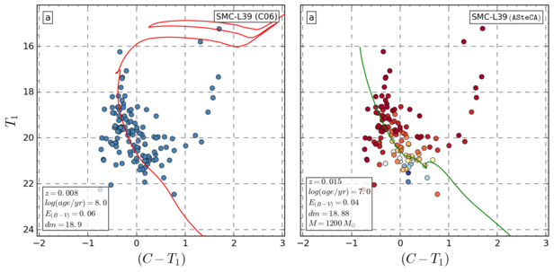
Figure 26: CMDs for the C06 database.

In Appendix C we show CMDs for the 153 cross-matched clusters across these four DBs. Clusters that present the largest age discrepancies between ASteCA and the DBs, are those where the same effect mentioned in Appendix B takes place. A good example of this is SMC-L39, as seen in Figs. 26 and 35 for C06 and G10 respectively.

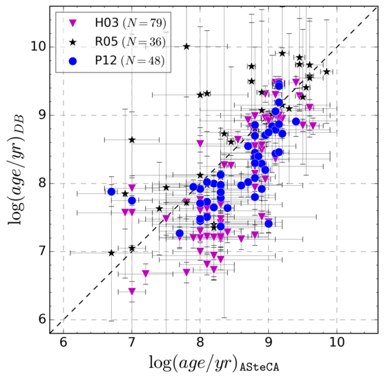
Figure 8: Age comparison for integrated photometry DBs versus ASteCA. $N$ is the number of clusters cross-matched in each DB.

Our age and mass estimates are also compared with three DBs – H03, R05, and P12 – which used integrated photometry (see Table 2). Only H03 and P12 obtained total mass values, these are analyzed in Sect. 5.2.1.

H03 studied approximately 1000 clusters, 196 and 748 in the S/LMC, via $UBVR$ integrated photometry. Ages were assigned based on the Starburst99 model (Leitherer et al., 1999), assuming metallicities, distance moduli, and average $E_{B-V}$ values of (0.004, 0.008), (18.94, 18.48) mag, and (0.09, 0.13) mag, for the S/LMC, respectively. Masses were derived from $M_{V}$ absolute magnitude and a mass-luminosity relation. This article represents, as far as we are aware, the largest published database of MCs cluster masses to date.

R05 used two models – GALEV (Anders & Fritze-v. Alvensleben, 2003) and Starburst99 – combined with three metallicities – (0.004, 0.008) and (0.001, 0.004, 0.008), used in each model respectively – to obtain five age estimates for 195 SMC clusters. Reddening values were assigned using fixed age ranges, following Harris & Zaritsky (2004). We averaged all reddening-corrected ages for each matched cluster, and assigned an error equal to the midpoint between the lowest and highest error.

P12 used the same dataset from H03 to analyze 920 LMC clusters through their MASSCLEAN_colors and MASSCLEAN_age packages (Popescu & Hanson, 2010b, a). Metallicities were fixed to $z{=}0.008$, while reddening is taken from G10 when available, or fixed to $E_{B-V}{=}0.13$ mag as done in H03. Ages and masses from duplicated entries in the P12 sample are averaged in our analysis.

As seen in Fig. 8, H03 underestimates ages for younger clusters. This effect was registered in de Grijs & Anders (2006, see Fig. 1), which the authors assigned to the photometry conversion done in H03. Average $\log(age/yr)$ dispersion between H03 and ASteCA is $0.44{\pm}0.56$ dex. The same happens for P12 ages, albeit with a smaller $\log(age/yr)$ dispersion of ${\sim}0.35{\pm}0.44$ dex. P12 compared their own age estimates with H03 (see P12, Fig. 8). They find a systematic difference with H03, where MASSCLEAN ages are larger for clusters with $\log(age/yr){<}8$ dex. In our case, most of the clusters cross-matched with P12 are older than 8 dex, with P12 ages located mostly below the identity line. This bias towards smaller age estimates by P12 is consistent with what was found in Choudhury et al. (2015). Contrary to the results found for H03 and P12, the R05 study slightly underestimates ages compared to ASteCA, with a mean $\log(age/yr)$ dispersion of $-0.25{\pm}0.63$ dex. The standard deviation is the largest for the three integrated photometry DBs. In R05 the authors mention the lack of precision in their age measurements, due to the use of integrated colors, and the lack of constrains for the metallicity.

Expectedly, the four isochrone fit studies analyzed previously show a more balanced distribution of ages around the 1:1 relation, in contrast with the integrated photometry DBs. Ages taken from integrated photometry studies are known to be less accurate, and should be taken as a rather coarse approximation to the true values. As shown in P12, integrated colors present large scatters for all age values, leading inevitably to degeneracies in the final solutions. The added noise by contaminating field stars is also a key issue, as it is very difficult to remove properly from integrated photometry data. A single overly bright field star can substantially modify the observed cluster’s luminosity, leading to incorrect estimates of its parameters (Baumgardt et al., 2013; Piatti, 2014). A detailed analysis of some of the issues encountered by integrated photometry studies, and the accuracy of their results, is presented in Anders et al. (2013).

5.2.1 Integrated photometry masses

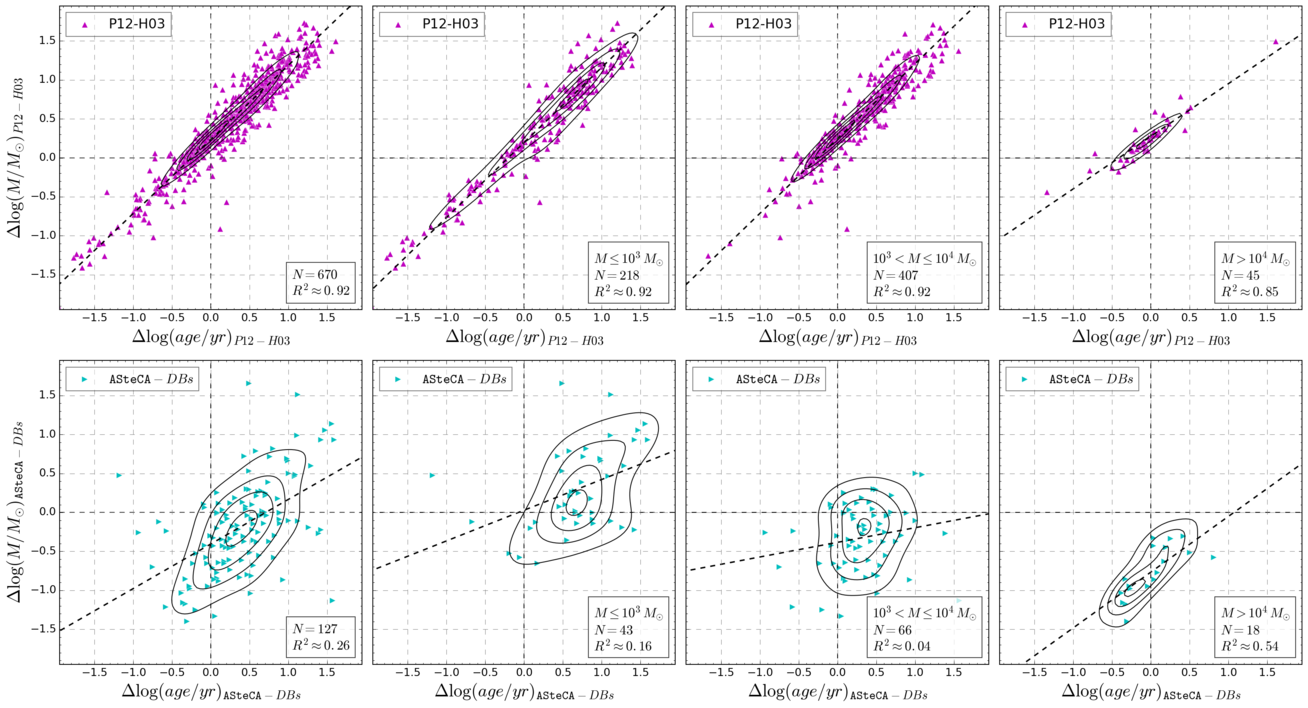
Figure 9: Top row: Differences plot $\log(age/yr)$ versus $\log(M/M_{\odot})$, for 670 P12 and H03 cross-matched clusters, in the sense P12 minus H03. A 2-dimensional Gaussian kernel density estimate is shown as iso-density black curves. The dashed line is the result of the best fit linear regression; the $R^{2}$ coefficient is shown in the bottom left box. The leftmost diagram shows all 670 clusters processed together, the remaining diagrams are divided by mass ranges. Bottom: idem, for ASteCA versus DBs (where DBs represent the mixed H03 and P12 sample) for the 127 cross-matched clusters.

Cross-matching the H03 and P12 DBs with a maximum search radius of 20 arcsec, results in 670 unique LMC clusters. In the top row of Fig. 9 we show the differences in mass and age estimates for both DBs. The leftmost diagram contains all the cross-matched clusters, while the other diagrams are sectioned by mass ranges. The three mass regions show how the age-mass correlation – an older large cluster is incorrectly identified as a much younger and less massive one or vice-versa – strongly affects estimates between these DBs. The mean value $\overline{\Delta M_{\log}}$ (logarithmic mass difference) decreases from $0.8{\pm}0.5$, to $0.3{\pm}0.5$, to $-0.4{\pm}1$; in the low, medium, and large mass regions defined in Fig. 9, respectively. Masses go from being overestimated a factor of ${\sim}6$ by P12 in the low mass region, to being underestimated by a factor of ${\sim}2.5$ in the large mass region. Where P12 estimates larger masses, it also assigns larger ages by more than 1.5 dex. Conversely, in the large average mass region, P12 ages can reach values up to 3 dex lower than H03. There are five clusters with H03 masses larger than $2.5{\times}10^{5}\,M_{\odot}$ in this cross-matched sample, all incorrectly assigned a low age and mass by P12. These five LMC globular clusters are: NGC1916, NGC1835, NGC1786, NGC1754, and NGC1898. P12 assigns masses below 2000 $M_{\odot}$ in all cases.

Cross-matching the H03 and P12 DBs with our sample, results in a set of 127 clusters. The age-mass positive correlation that was obvious for H03 and P12, is not present when we compare DBs masses and ages estimates with those from ASteCA, as seen in the bottom row of Fig. 9.

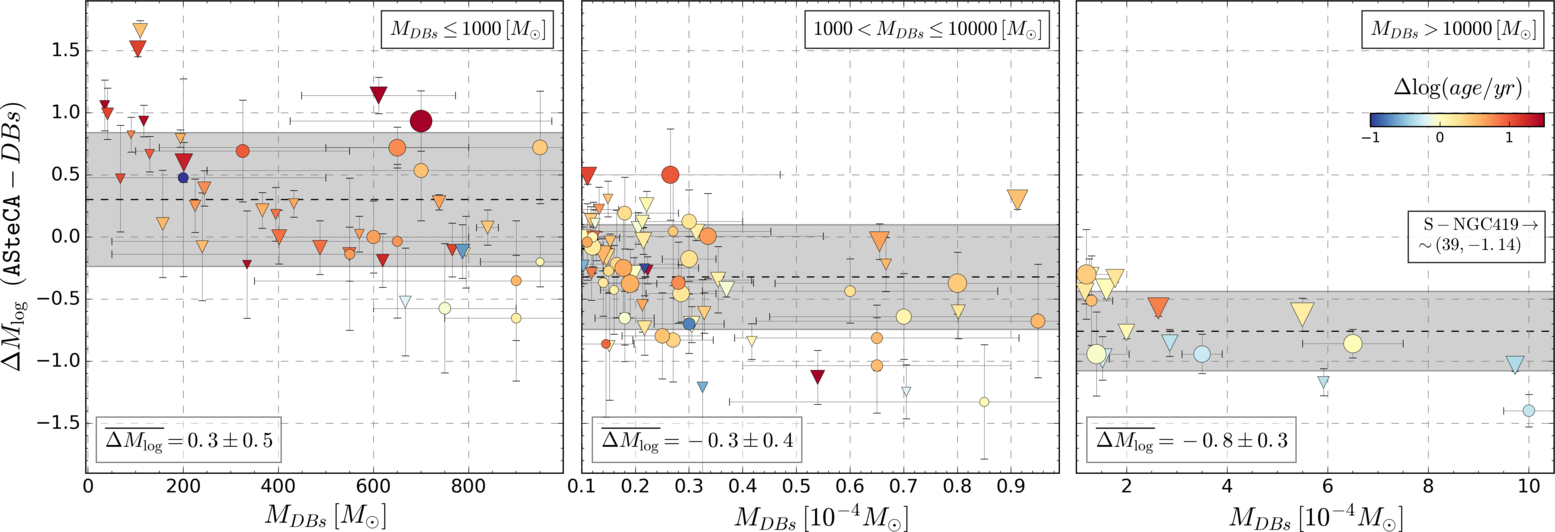
Figure 10: Left: BA mass plot, showing the differences between estimated masses in the H03 and P12 DBs and the code, in the sense ASteCA minus DB; symbols as in Fig. 8. Only DB masses ${\leq}10^{3}\,M_{\odot}$ are shown here. Colors are assigned according to the difference in $\log(age/yr)$ estimation of each cluster (ASteCA minus DB, colorbar is shown in the right plot), while sizes are proportional to the actual sizes in parsecs. The horizontal dashed line ($\overline{\Delta M_{\log}}$) is the mean of the combined logarithmic differences. The gray band is the ${\pm}1\sigma$ region for this mean. Center: same as previous plot, now showing DB mass values in the range $10^{3}-10^{4}\,M_{\odot}$. Right: same as previous plot, for DB mass values ${>}10^{4}\,M_{\odot}$.

In Fig. 10 we show masses for the 127 cross-matched clusters in these DBs, versus their logarithmic mass differences. The mean standard mass difference $\Delta M$ (${=}M_{\mathtt{ASteCA}}-M_{DBs}$) is ${\sim}40{\pm}1700\,M_{\odot}$ for $M_{DBs}{<}5{\times}10^{3}\,M_{\odot}$, and ${\sim-}400{\pm}2500\,M_{\odot}$ for $M_{DBs}{<}10^{4}\,M_{\odot}$; pointing to a very reasonable scatter around the identity line. Although the standard deviation values are somewhat large, this is expected for a set of clusters in this mass range. As stated in Baumgardt et al. (2013) and P12, clusters with $M{\lesssim}5{\times}10^{3}-10^{4}\,M_{\odot}$ tend to have their estimated integrated photometry masses largely dominated by stochastic processes.

We see in Fig. 10 that the larger the DB mass, the larger the logarithmic difference with ASteCA. Values for $\overline{\Delta M_{\log}}$ in the medium and large-mass regions of Fig. 10 mean that DB masses are between two and six times larger than ASteCA masses. The most discrepant case is that of SMC-NGC419 – left out of the right plot for clarity – which shows a mass of $3.9{\times}10^{5}\,M_{\odot}$ by H03, and $2.8{\times}10^{4}\,M_{\odot}$ by the code.

After exploring several possible processes that could induce this systematic mass difference – between our estimates and those from integrated photometry studies–, we concluded that the responsible is the effect of stellar crowding in our Washington photometry. The likelihood defined in Eq. 1 is a binned statistic. This means that stars not accounted for in the CMD will bias the mass estimation, as it depends on the number of observed stars. The larger the number of stars lost because of this process, the larger the underestimation of mass for a given observed cluster. To test the above hypothesis, we requested the HST data used in Goudfrooij et al. (2014) to analyze NGC419. The ACS/WFC instrument – from where this data comes from – has a much higher resolution compared to that from our Washington photometry (0.05 arcsex/pixel versus 0.274 arcsec/pixel), so we can expect a substantially lower percentage of stars lost. The authors estimate a mass of ${\sim}2.4{\times}10^{5}\,M_{\odot}$ using a Salpeter (1955) IMF (which could be as low as ${\sim}1.5{\times}10^{5}\,M_{\odot}$ if a more recent IMF was used). We analyzed this dataset with ASteCA fixing all parameters to the values given in Goudfrooij et al., with the exception of the mass which was left to vary up to $3{\times}10^{5}\,M_{\odot}$. A cut on $F555W{=}23$ mag was imposed to minimize the impact of faint stars lost due to crowding. The mass found this way for NGC419 is $2.5{\times}10^{5}\,M_{\odot}$, a very similar value to the average of H03 and Goudfrooij et al ($2.6{\times}10^{5}\,M_{\odot}$). It is thus clear that stellar crowding in our low resolution photometry is the responsible for the systematic difference in estimated masses.

Even though ASteCA corrects synthetic clusters using a completeness function – approximated from the observed cluster’s LF–, this only affects the faintest synthetic stars. For heavily crowded clusters (especially if they are observed with low resolution) this underestimates the loss of brighter stars which intensifies as one moves closer to the cluster’s center (Mateo, 1988), hence underestimating its mass. Future releases of the code will allow the user to input a manual completeness function, ideally obtained through proper artificial star tests (see e.g., Aparicio & Gallart, 1995). Mass values obtained in the present study for massive clusters, should therefore be considered lower estimates of their true value.

6 Fundamental parameters in the analyzed database

We present a summary of the distribution of the five fundamental parameters obtained with ASteCA, for the 239 MCs clusters in our catalog. A method is devised in Sect. 6.1 to allow an unbiased analysis of the estimated values, and the results presented in Sect. 6.2. Reddenings, distances, and total masses do not span sufficiently large ranges to account for the values found in the MCs. Their distribution can thus only be though to characterize the state of those clusters in this catalog. On the other hand, metallicities and ages obtained cover a wide range in both galaxies. Their distribution can be regarded as a representative randomized sample of the cluster system in the MCs. Their relationship is studied in Sect.6.3.

6.1 Method

Histograms are used to derive a large number of properties in astrophysical analysis, for example a galaxy’s star formation history (SFH). Their widespread use notwithstanding, the generation of a histogram is affected by well known issues (see Silverman, 1986; Simonoff & Udina, 1997). Different bin widths and anchor positions can make histograms built from the same data look utterly dissimilar. In the worst cases, completely spurious sub-structures may appear, leading the analysis towards erroneous conclusions. We bypass these issues by constructing an adaptive (variable) Gaussian kernel density estimate (KDE) in one and two dimensions, using the parameters’ standard deviations as bandwidth estimates. The formulas for both KDEs are:

$$KDE_{1D}(x)=\frac{1}{N\sqrt{2\pi}}\sum_{i=1}^{N}\frac{1}{\sigma_{i}}e^{-\frac{(x-x_{i})^{2}}{2\sigma_{i}^{2}}},$$ (4)

$$KDE_{2D}(x,y)=\frac{1}{2\pi N}\sum_{i=1}^{N}\frac{1}{\sigma_{xi}\sigma_{yi}}e^{-\frac{1}{2}\left(\frac{(x-x_{i})^{2}}{\sigma_{xi}^{2}}+\frac{(y-y_{i})^{2}}{\sigma_{yi}^{2}}\right)},$$ (5)

where $N$ is the number of observed values, $x_{i}$ is the $ith$ observed value of parameter $x$, and $\sigma_{xi}$ its assigned standard deviation (same for $y_{i}$ and $\sigma_{yi}$). The 1D version of these KDEs is similar to the “smoothed histogram” used in the Rafelski & Zaritsky (2005) study of SMC clusters. Using standard deviations as bandwidth estimates means that the contribution to the density map of parameters with large errors, will be smoothed (“spread out”) over a large portion of the domain. Precise parameter values on the other hand, will contribute to a much more narrow region.

Replacing one and two-dimensional histogram analysis with these KDEs has two immediate benefits: a) it frees us from having to select an arbitrary bandwidth value (the most important component of a KDE), and b) it naturally incorporates errors obtained for each parameter into its probability density function.

6.2 Distribution of parameters within the observed ranges

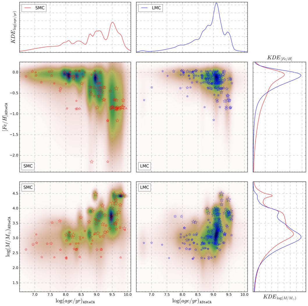
Figure 11: Adaptive Gaussian KDEs for age, metallicity, and mass. Top and right plots are 1D KDEs, center plots are 2D KDEs. Observed clusters are plotted as red and blue stars for the S/LMC, respectively. Sizes are scaled according to each cluster’s radius. A small scatter is introduced for clarity.

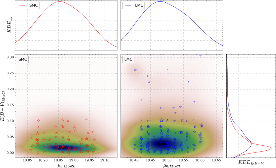
Figure 12: Same as Fig. 11 for $E_{(B-V)}$ and distance modulus.

Figs. 11 and 12 show 1D and 2D density maps constructed via Eqs. 4 and 5. A distinct period of cluster formation is visible in the LMC around ${\sim}$5 Gyr, which culminated ${\sim}$1.3 Gyrs ago. A similar but less pronounced peak is seen for the SMC, with a drop in cluster formation around ${\sim}$2 Gyr. Height differences between the SMC and LMC KDEs, is related to the relative decline in cluster formation. While the LMC sharply drops to almost zero from ${\sim}$1 Gyr to present times, the SMC shows a softer descent with smaller peaks around ${\sim}$250 Myr and ${\sim}$130 Myr. The well known “age gap” in the LMC between 3–10 Gyrs (Balbinot et al., 2010) is present, visible as a marked drop in the $KDE_{\log(age/yr)}$ curve at $\sim 9.5$ dex.

The 2D KDE age-metallicity map shows how spread out these values are for clusters in the SMC, compared to those in the LMC. Although the SMC abundance reaches substantially lower values, the right 1D KDE reveals [Fe/H] peaks between 0 dex and -0.2 dex, for clusters in both Clouds.

The age-mass 2D map shows a clustering around younger ages and smaller masses for the LMC. The SMC cluster seen in the bottom right corner is HW42 ($\alpha{=}1^{h}01^{m}08^{s}$, $\delta{=}-74^{\circ}04^{\prime}25^{\prime\prime}$ [J2000.0]), a small cluster (radius ${<}20$ pc) located close the the SMC’s center. Though its position in the map is somewhat anomalous, the 1$\sigma$ error in its age and mass estimates could move it to $\log(age/yr){\simeq}9.4$ and $\log(M/M_{\odot}){\simeq}2.6$. This cluster is classified as a possible emissionless association by Bica & Schmitt (1995). There is a tendency in both Clouds for the clusters’ mass and size to grow with estimated age, as expected (due to the mass-to-light ratio increase with age; see Popescu et al., 2012, Sect. 4).

As seen in Fig. 12 (top), the 1D KDEs of the distance moduli are well behaved and normal in their distribution. A Gaussian fit to these curves results in best fit values of 18.96$\pm$0.08 mag and 18.49$\pm$0.08 mag for the S/LMC. Literature mean distances are thus properly recovered. Reddening values are much more concentrated in the sample of SMC clusters around $E_{B-V}{\approx}0.015$ mag. LMC reddenings are dispersed below $E_{B-V}{\approx}0.1$ mag, with a shallower peak located at ${\sim}0.03$ mag.

6.3 Age-metallicity relation

A stellar system’s age-metallicity relation (AMR) is an essential tool to learn about its chemical enrichment evolution. In Piatti (2010) an AMR method was devised using age bins of different sizes, to take age errors into account. It was applied to derive AMRs in Piatti & Geisler (2013), and adapted to obtain star cluster frequency distributions in Piatti (2013). We propose a new method based on the KDE technique described in Sect. 6, with a number of advantages over previous ones. Mathematical details are given in Appendix D, where the method is applied to generate AMRs using literature age and metallicity values.

ASteCA AMRs for the S/LMC can be seen in Fig. 13 as red and blue continuous lines, respectively. Stars show the position of all clusters in our sample, with sizes scaled according to their radii. Shaded regions represent the 1$\sigma$ standard deviations of the AMRs, spanning a [Fe/H] width of ${\sim}0.2$ dex for the entire age range, for both Clouds. The blue (top) and red (bottom) vertical segments in the top plot are the bin edges determined for each age interval by Knuth’s algorithm. The final AMR functions are mostly unaffected by the chosen binning method. Using Knuth’s algorithm results in ${sim}11$ age intervals of widths between 0.35 and 1 Gyr, as seen in Fig. 13. If instead we use 100 intervals of ${\sim}0.1$ Gyr width, only the SMC curve is perturbed in the region $\mathrm{Age}{<800}$ Myr where [Fe/H] values are raised by ${\sim}0.1$ dex. If the two SMC clusters with very low metal abundances ([Fe/H]${<-}2$ dex) are excluded from our data, the AMR moves upwards in the [Fe/H] axis by less than 0.05 dex, for ages below 500 Myr.

Several chemical evolution models and empirical AMRs are found in published articles. We show in Fig. 13 – center and bottom plots – AMR functions presented in twelve other works.

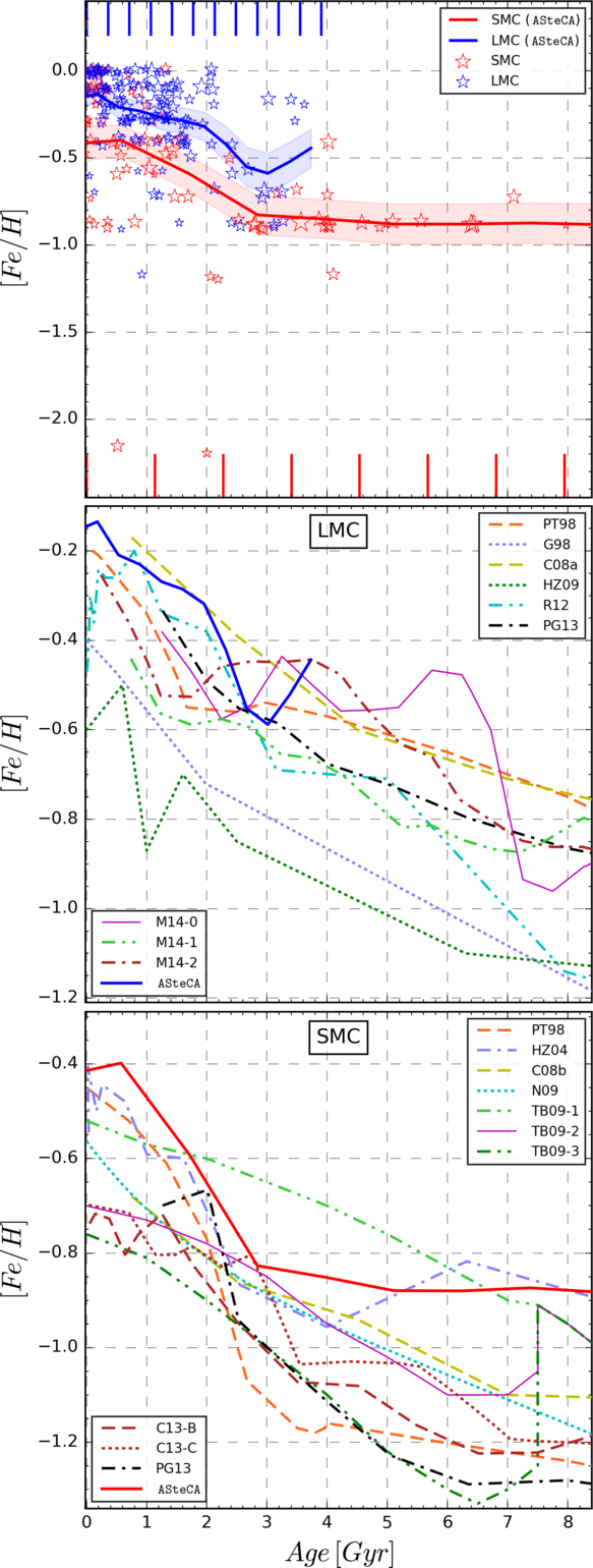
Figure 13: ASteCA’s age-metallicity relation for the S/LMC (red/blue solid lines). See text in Sect. 6.3 for more details.

These external studies constitute a representative sample of the different methods and data used over the past twenty years: Pagel & Tautvaisiene (1998, PT98; bursting models), Geha et al. (1998, G98; closed-box model with Holtzman SFH), Harris & Zaritsky (2004, HZ04), Carrera et al. (2008b, C08a; average of four disk frames), Carrera et al. (2008a, C08b; average of thirteen frames), Harris & Zaritsky (2009, HZ09), Noël et al. (2009, N09; 5th degree polynomial fit to the AMRs of their three observed regions), Tsujimoto & Bekki (2009, TB09; 1: no merger model, 2: equal mass merger, 3: one to four merger), Rubele et al. (2012, R12; four tiles average), Cignoni et al. (2013, C13; B: Bologna, C: Cole), Piatti & Geisler (2013, PG13), and Meschin et al. (2014, M14; 0: field LMC0, 1: field LMC1, 2: field LMC2). Details on how these AMRs were constructed can be consulted in each reference. All of the above mentioned articles used field stars for the obtention of their AMRs. This is, as far as we are aware, the first work were the AMR function for both galaxies is derived entirely from observed star clusters.

The AMRs’ trend coincides with what has already been found, namely that the metallicity increases for younger ages (particularly below 3 Gyr). On average, our AMR estimates are displaced slightly towards more metal rich values. Most [Fe/H] values in the external studies are obtained using a solar metallicity of $z_{\odot}{=}0.019$, while we used the more recent value $z_{\odot}{=}0.0152$. As was shown in Sect. 5.1, this difference means [Fe/H] estimates will be ${\sim}0.1$ dex smaller for external studies.

For the LMC galaxy, Fig. 13 center plot, we see a marked drop in metallicity from ${\sim-}0.45$ dex beginning around 3.8 Gyr, and ending 3 Gyrs ago at ${\sim-}0.6$ dex. The M14-0 curve seems to reproduce this behavior, but shifted ${\sim}0.8$ Gyr towards younger ages. This high metallicity value of the LMC’s AMR at its old end, is caused by the three clusters with [Fe/H]${\approx-0.2}$ dex located beyond ${\sim}3.5$ Gyr; the oldest ages estimated by ASteCA. Without any older clusters available in the LMC, it is hard to assess whether this is a statistically significant feature of the AMR. After the drop, there is a steep climb from 3 Gyr to 2 Gyr reaching almost [Fe/H]${\sim-}0.3$ dex, and then a sustained shallower increase up to the estimated present day’s metal content of ${\sim-}0.15$ dex. Our average metallicity value for present day clusters coincides reasonably well with the PT98 bursting model, which shows nonetheless a very different rate of increase from 2 Gyr to present times. The C08a AMR, while lacking finer details, provides a better match for this age range. The HZ09 and G98 AMRs differ the most not only from the ASteCA AMR, but from the rest of the group.

The SMC ASteCA AMR is shown along ten published AMRs in Fig. 13, bottom. The peak around ${\sim}7.5$ Gyr predicted by TB09 in its two merger models (1:1, and 1:4 merger) is not visible in our AMR. ASteCA’s AMR remains largely stable around a value of [Fe/H]${\simeq-}0.9$ dex until approximately 3 Gyrs ago, where the rate of growth increases considerably. From that point up to the present day, the average metallicity for clusters in the SMC grows by ${\sim}0.4$ dex. The abundance increase for ages ${<}3$ Gyrs, is only reproduced by the PT8 model, and the HZ04 function. The PT98 model starts diverging from our AMR at ${\sim}2$ Gyr, until a gap of ${\sim}0.4$ dex in [Fe/H] is generated. In contrast, the HZ04 curve remains much closer to our own throughout the entire age range. These two AMRs estimate a present day metallicity very close to the [Fe/H]${\approx}-0.4$ dex value estimated by ASteCA.

Overall, our AMRs can not be explained by any single model or empirical AMR function, and are best reproduced by a combination of several. A similar result was found in Piatti & Geisler (2013) although their field stars AMRs are significantly different from ours, mainly for the SMC. It is important to remember that ASteCA’s AMRs are averaged over the structure of both Magellanic Clouds. In Fig. 1 we showed that our set of clusters covers a large portion of the surface of these galaxies. If more clusters where available so that the AMRs could be estimated by S/LMC sectors, it is possible that different results would arise.

7 Summary and conclusions

We presented an homogeneous catalog of 239 star clusters in the Large and Small Magellanic Clouds, observed with the Washington photometric system. The clusters span a wide range in metallicity and age, and are spatially distributed throughout both galaxies. The fundamental parameters metallicity, age, reddening, distance modulus, and total mass were determined using the ASteCA package. This tool allows the automated processing of a cluster’s positional and photometric data, resulting in estimates of both its structural and intrinsic/extrinsic properties. As shown in Paper I, the advantages of using ASteCA include reproducible and objective results, along with a proper handling of the uncertainties involved in the synthetic cluster matching process. This permits the generation of a truly homogeneous catalog of observed clusters, with their parameters fully recovered. Our resulting catalog is complete for all the analyzed parameters, including metallicity and mass, two properties often assumed or not obtained at all.

Internal errors show no biases present in our determination of fundamental parameters, as seen in Sect. 4. The analysis of our results in Sect. 5.1, demonstrate that the assigned values for the clusters are in good agreement with published literature which used the same Washington photometry. Metallicity was the most discrepant parameter, with ASteCA’s [Fe/H] values on average ${\sim}0.22$ dex larger than those present in the literature. Half of this difference is due to the solar abundance used in this work. The remaining ${\sim}0.1$ dex is explained by the confirmation bias effect in most cluster studies, that will assume canonical [Fe/H] values rather than derive them through statistically valid means. We also compared our results with articles that used different photometric systems, in Sect. 5.2. While the age differences in this case are somewhat larger, they can be mostly explained by effects outside the code.

We performed in Sect. 5.2.1 a detailed comparative study of masses obtained through integrated photometry studies, with our own estimates from CMD analysis. Although for smaller clusters the estimation is reasonable, mass values are systematically underestimated for larger clusters, due to the effect of stellar crowding in our own photometry.

A method for deriving the distribution of any fundamental parameter – or a combination of two of them – is presented in Sect. 6.1. It takes into account the information contained by the uncertainties, often excluded from the analysis. By relying on Gaussian kernels, it is robust and independent of ad-hoc binning choices. An age-metallicity relation is derived in Sect. 6.3, for cluster systems in both galaxies. The AMRs generated can not be fully matched by any model or empirical determination found in the recent literature.

We demonstrated that the ASteCA package is able to produce proper estimations for the fundamental parameters of observed star clusters, within the limitations imposed by the photometric data. A necessary statistically valid error analysis can be performed, thanks to its built-in bootstrap error assignment method. The tool is proven capable of operating almost entirely unassisted, on large databases of clusters. This is an increasingly essential feature of any astrophysical analysis tool, given the growing importance of big data and the necessity to conduct research on large astronomical data sets.

Appendix A Total cluster mass validation

The likelihood used in this work (Eq. 1) allows to set the total cluster mass as a free parameter to be optimized. To validate ASteCA’s mass recovery we processed 768 synthetic clusters generated with the MASSCLEAN tool, 384 for each Magellanic Cloud. These clusters imitate the metallicity, and age range for clusters in both Clouds, with a large maximum mass. The distance and reddening parameters were fixed; see table 4. The process of generating a MASSCLEAN cluster was described in Paper I, Sect. 3. It is worth noting that these clusters are affected by stellar crowding, only in their faintest magnitudes (using a theoretical completeness function similar to that presented in Small et al. 2013). As such, their mass estimations will not suffer from the systematic underestimation seen in Sect. 5.2.1. Each MASSCLEAN cluster had its $V$ vs ($B-V)$ CMD (in the $UBRIJHK$ photometric system) analyzed by ASteCA.

Table 4: Parameter values used to generate the set of 768 MASSCLEAN clusters.

Parameter	Values	N
z	0.001, 0.004, 0.015, 0.03	4
$\log\mathrm{(age/yr)}$	7, 7.2, 7.5, 7.7, 8, 8.2, 8.5, 8.7, 9, 9.2, 9.5, 9.7	12
$\mu_{0}$	18.9 (SMC), 18.5 (LMC)	2
$E_{B-V}$	0.1	1
Mass ($M_{\odot}$)	500, 1000, 5000, 10000, 25000, 50000, 100000, 250000	8

In Fig 14 we show the masses recovered for the 768 MASSCLEAN clusters. The x-axis displays the true MASSCLEAN mass values. The y-axis shows the logarithmic mass differences, in the sense ASteCA minus MASSCLEAN. Colors follow the differences in $\log(age/yr)$ (ASteCA minus MASSCLEAN), shown in the right plot colorbar. Average age differences for each mass region are: $-0.3{\pm}0.6$ dex ($\overline{M}{\leq}1000\,[M_{\odot}]$), $-0.05{\pm}0.19$ dex ($1000{<}\overline{M}{\leq}10000\,[M_{\odot}]$), $-0.01{\pm}0.13$ dex ($\overline{M}{>}10000\,[M_{\odot}]$). As expected, clusters with larger masses have their ages more accurately recovered. On average, the difference between ASteCA (estimated) minus MASSCLEAN (true) logarithmic ages in the full mass range is ${\sim}-0.1{\pm}0.4$ dex. Gray bands represent the mean and standard deviation for the logarithmic mass differences, $\overline{\Delta M_{\log}}$. For low mass clusters – $500\,M_{\odot}$ or $1000\,M_{\odot}$ – the code assigns masses in a range between ${\sim}200{-}3000$ $M_{\odot}$. In this region ASteCA underestimates clusters’ masses by ${\sim}200\,M_{\odot}$. This effect is tied to an improper age estimation, where ASteCA incorrectly assigns younger ages to scarcely populated clusters, and compensates the low number of stars by decreasing the total mass. Such an issue is not unexpected for very low mass clusters.

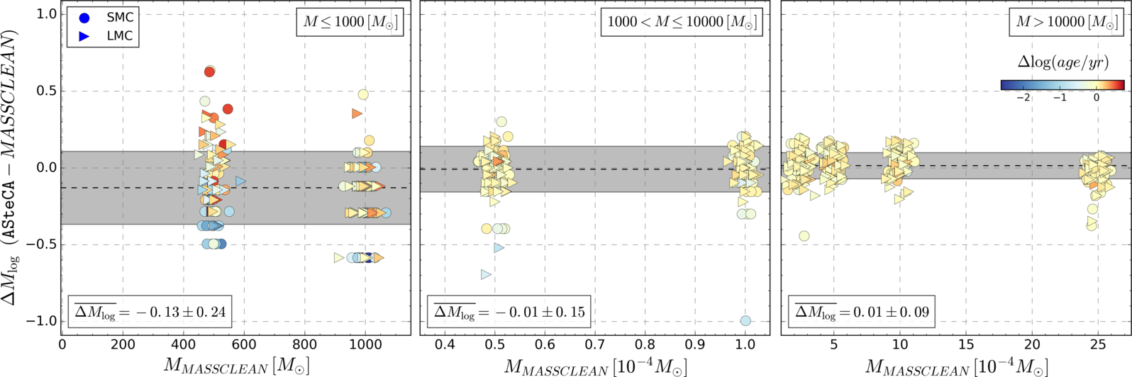
Figure 14: Recovered masses by ASteCA for the 768 MASSCLEAN clusters. Logarithmic mass differences $\Delta M_{\log}$ are obtained in the sense ASteCA minus MASSCLEAN, and shown in the y-axis. MASSCLEAN masses in the x-axis are perturbed with a small random scatter.

Table 5 shows the correlation matrix between the five cluster parameters. We see the usual correlations appear (age-metallicity, metallicity-distance, age-reddening, etc.), as found in Paper I (Table 3). Total mass shows a small positive correlation with the distance modulus. When distance is overestimated, the matched synthetic CMD will contain fewer low mass stars due to the magnitude limit. The likelihood will compensate this loss by increasing its mass.

Table 5: Correlation matrix for parameter deltas, defined for each cluster in the sense ASteCA minus MASSCLEAN.

$\Delta param$	$\Delta z$	$\Delta\log(age/yr)$	$\Delta\mu$	$\Delta E_{B-V}$	$\Delta M$
$\Delta z$	1.	-0.36	0.24	-0.15	0.03
$\Delta\log(age/yr)$	–	1.	-0.15	-0.28	0.01
$\Delta\mu$	–	–	1.	0.05	0.13
$\Delta E_{B-V}$	–	–	–	1.	0.0
$\Delta M$	–	–	–	–	1.

A.1 Metallicity estimation for different mass values

The metallicity ($z$) estimated for the MASSCLEAN set is displayed in Fig. 15, where tendencies are visible. First, as the cluster’s mass grows so does the accuracy of the metallicity estimates. Although the average difference between true and estimated values remains close to $\overline{\Delta z}{\approx}0.001$ for the entire mass range – this is expected, as $z{=}0.001$ is the step used by ASteCA –, its standard deviation drops from ${\sim}0.01$ to $0.004$ for the more massive clusters. Most of the poorest solutions obtained by ASteCA – those with $|\Delta z|{>}0.01$ dex – are associated to low mass scarcely populated clusters, with ${\sim}40$ true member stars on average (from two up to a hundred) in their analyzed CMDs. This poor solutions set is composed of 91 clusters – ${\sim}12\%$ of the sample – 58 of which have $M{\leq}1000\,M_{\odot}$. Of these 58 low mass clusters, 38 are assigned younger ages by the code due to an improper field star decontamination process (an expected issue when the number of true members is very low). Of the 82 clusters with the worst age estimates by ASteCA – $|\Delta\log(age/yr)|{\geq}0.5$ dex, ${\sim}11\%$ of the MASSCLEAN sample – ${\sim}90\%$ (73) are clusters with $M{\leq}1000\,M_{\odot}$. Leaving out these 82 clusters, the average difference in $z$ for the entire mass range is ${\sim}0.0008{\pm}0.006$ dex; a rather small difference with reasonable dispersion.

The second tendency is the overestimation of $z$ for the lowest metallicities, and its underestimation for the largest ones. A balanced distribution around $\Delta z{=}0$ line is mostly seen for abundances in the middle portion of the analyzed range. This trend is more noticeable for lower masses, but can be found for all mass values. This is a statistical artifact that arises due to the necessarily limited metallicity range analyzed. For clusters with the lowest metal contents ($z{=}0.001$), ASteCA can only assign equal or larger metallicities since negative $z$ values are not possible. Equivalently, for clusters with the largest abundances ($z{=}0.03$) the code can only associate equal or lower metallicities because of the upper $z$ limit used by ASteCA, which is precisely $z{=}0.03$. This “bias” could be avoided for large metallicity clusters, by increasing the $z$ range upper limit. It can not be avoided for the lowest metal abundances.

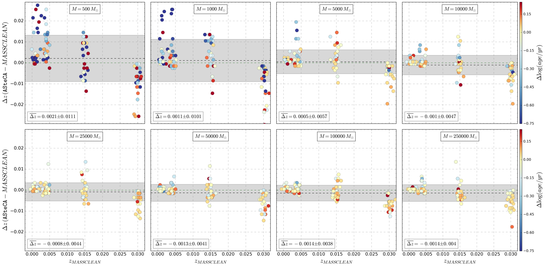
Figure 15: ASteCA metallicity estimates for each mass used to generate MASSCLEAN clusters. Colors are associated to $\log(age/yr)$ differences, shown in the colorbars to the right. The green dashed horizontal line is the $\Delta[Fe/H]{=}0$ line, shown as reference.

An external source of errors also needs to be taken into account when analyzing ASteCA’s metallicity (and age) estimates, for MASSCLEAN clusters. This is the intrinsic differences between Marigo et al. (2008) isochrones – used to generate MASSCLEAN clusters – and PARSEC (Bressan et al. 2012) isochrones – used by ASteCA to find the optimal fundamental parameters. These differences are a source of error in the matching process that is not straightforward to quantify. The two sets of tracks have non-negligible dissimilarities beyond the turn-off points, for most of the age range where they can be produced. This can be seen in Fig. 16, where isochrones from both sets are compared for five different $\log(age/yr)$ values from 7.5 to 9.5 dex. For ages up to 8 dex, PARSEC isochrones present a turn-off point located at lower $\log(L/L_{\odot})$ values, particularly for lower metallicities. This causes a shift in the more evolved portions of the isochrone, displacing the Marigo isochrones towards larger $\log(L/L_{\odot})$ values. Beyond that age this effects reverses, and PARSEC isochrones are now lifted above the Marigo tracks. Given the many known correlations between fundamental parameters it is not easy to predict how the matching algorithm will resolve such instances.

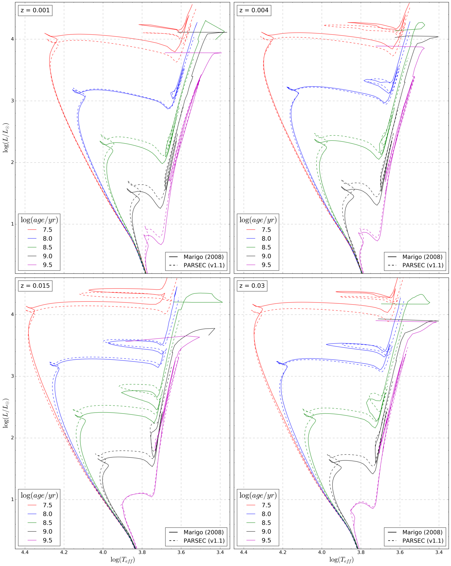
Figure 16: Marigo et al. (2008) versus PARSEC (Bressan et al. 2012) isochrones, for different metallicities and ages.

Appendix B Outliers

Ten of the analyzed clusters in this work – ${\sim}4\%$ of the set – show age differences with the literature $\Delta\log(age/yr){>}0.5$. Such a large age difference translates into two very dissimilar isochrones fitted to the same coeval star sequence, which makes this sub-sample of clusters stand out. For these “outliers” no configuration of the DA plus the employed binning methods could be found, that resulted in synthetic CMD matches with age values close to those found in the literature. All clusters in the outliers sample had smaller ages assigned by the code, compared to the literature, see Table  6. These differences go from 0.55 dex up to 1.6 dex in the most extreme case of LMC-KMHK975.

Table 6: Clusters with large age differences between the literature and values found by the code (“outliers”). Equatorial coordinates are expressed in degrees for the $J2000.0$ epoch. Ages are given as $\log(age/yr)$ for literature (L) and ASteCA (A). The difference between both estimates (L-A) is given in the last column as $\Delta$.

Cluster	$\alpha(^{\circ})$	$\delta(^{\circ})$	L	A	$\Delta$
L-KMHK975	82.49583	-67.87889	8.30	6.70	1.60
L-SL579	83.55417	-67.85639	8.15	7.00	1.15
L-BSDL631	76.64167	-68.42722	8.35	7.50	0.85
L-KMHK979	82.41250	-70.98389	7.90	7.30	0.60
L-H88-316	85.41250	-69.22944	8.25	7.70	0.55
S-L35	12.00417	-73.48611	8.34	6.90	1.44
S-H86-188	15.05833	-72.45833	8.10	6.70	1.40
S-L39	12.32500	-73.37167	8.05	7.00	1.05
S-B134	17.25417	-73.20667	8.15	7.20	0.95
S-K47	15.79583	-72.27361	7.90	7.00	0.90

In Fig. 17 CMDs for these clusters are plotted, two per row. Each CMD pair shows the cluster region with the literature isochrone fit (left), and the best match isochrone found by ASteCA (right). Colors in the right CMD correspond to the MPs assigned by the DA, while semi-transparent stars are those removed by the cell-by-cell density based cleaning algorithm (see Sect.3.3).

For most of the outliers, the same process is identified as the main cause responsible for the observed age differences. While the literature by-eye isochrone fit aligns the brighter part of the cluster’s sequence with the turn off point of a an older isochrone, ASteCA decides instead that this is the top portion of a much younger isochrone with no discernible turn off. The statistical mismatch due to the removal of low mass stars by the DA – discussed in Sect. 5.1 – can also be seen to affect some of the fits. In particular, SMC clusters SL579 and H86-188 show signs of this effect in the best synthetic CMD match selected by ASteCA (see Fig. 17, CMDs b and h).

These age estimates could be brought closer to literature values, if a more restrictive age range was used (e.g.: a minimum value of $\log(age/yr){=}7.5$ dex instead of 6 dex as used in this work). Lacking external evidence to substantiate this a priori restriction, we choose to keep the values obtained by ASteCA, with this section acting as a cautionary note.

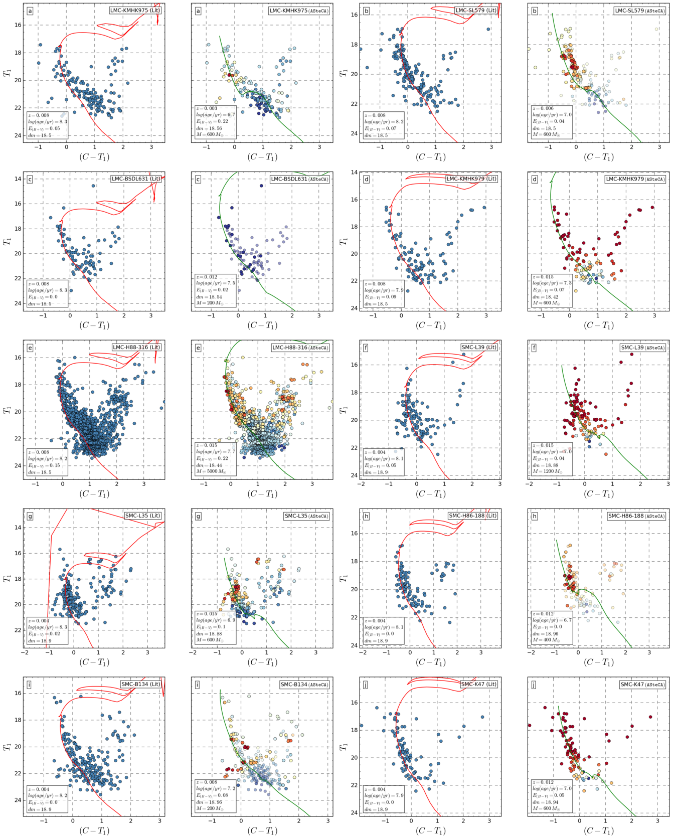
Figure 17: CMDs for the outliers set. Description of the plots in the main text of the section.

Appendix C Color-magnitude diagrams for the P99, P00, C06, and G10 databases

Figs. 18 to 35 present the CMDs of clusters cross-matched with our own sample in the databases P99, P00, C06, and G10, i.e.: those that used the isochrone fit method in their analysis. Same data distribution in the plotted CMDs as that described for Fig. 17.

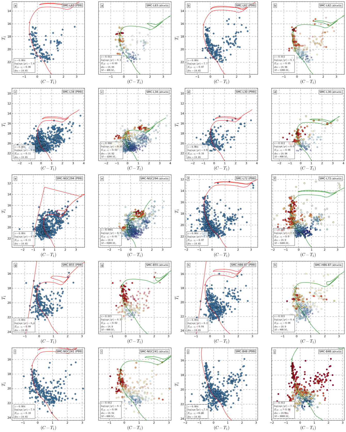
Figure 18: CMDs for the P99 database.

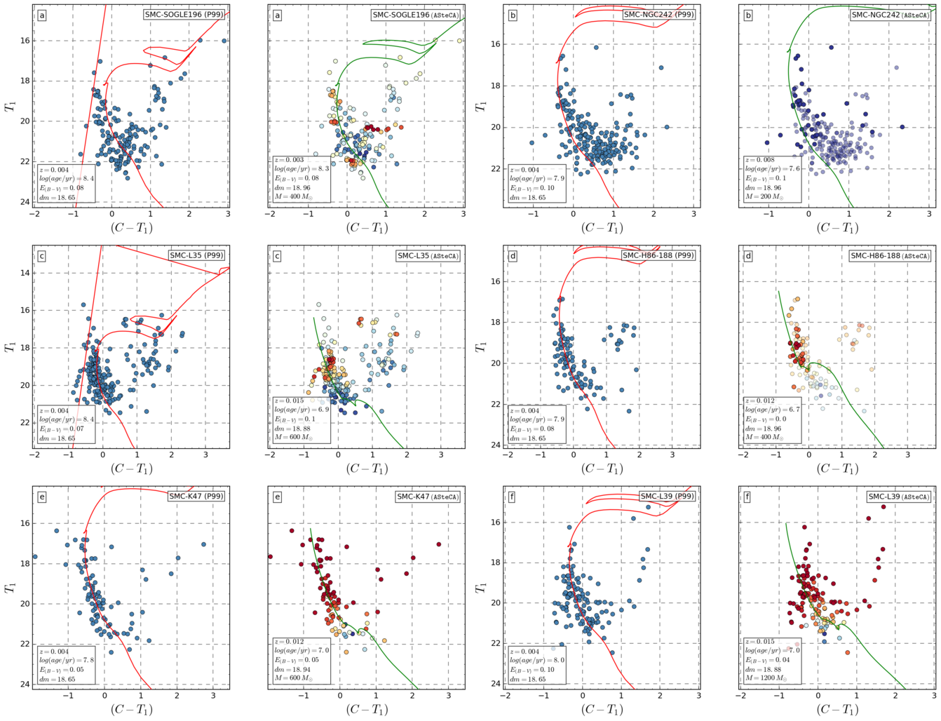
Figure 19: CMDs for the P99 database.

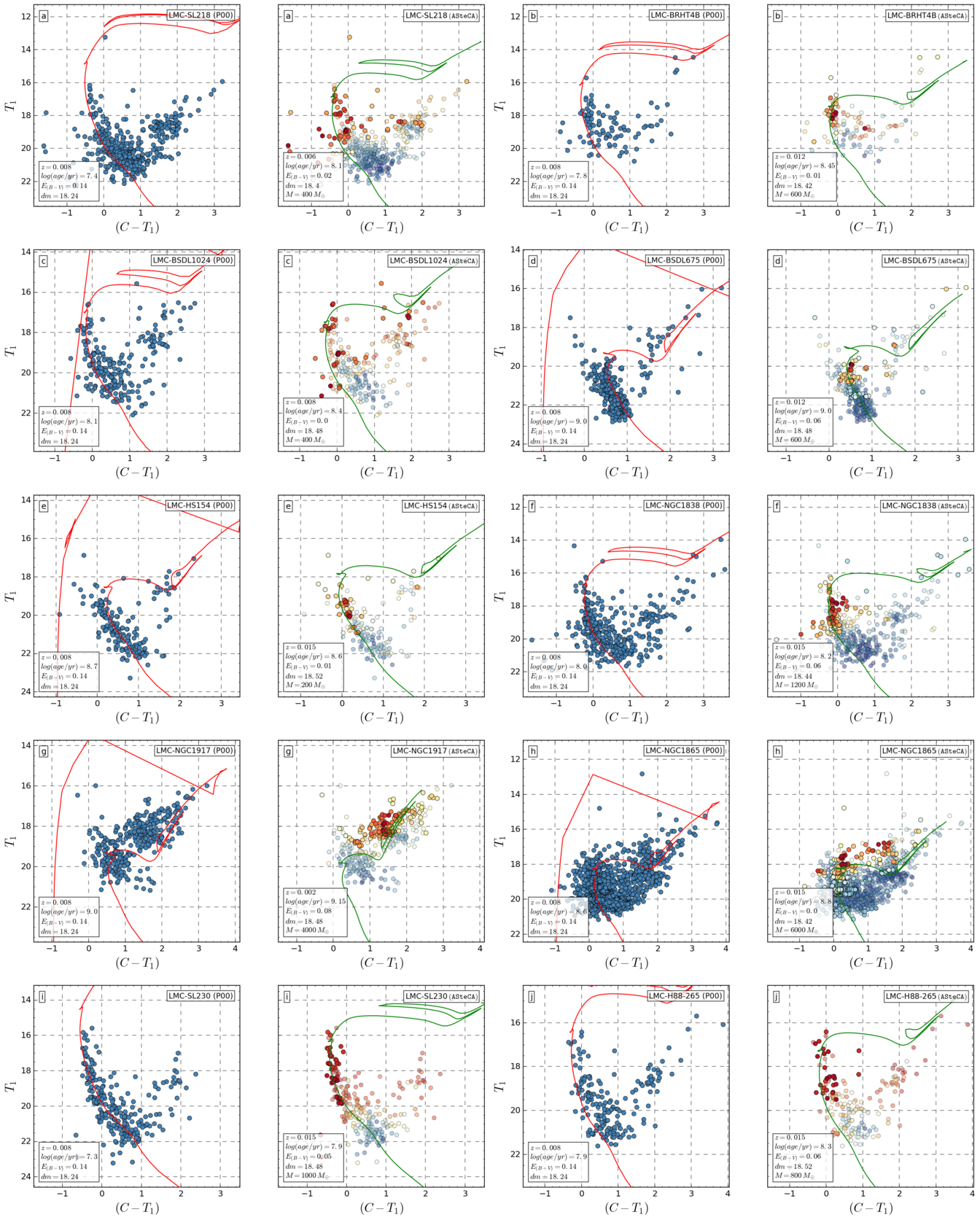
Figure 20: CMDs for the P00 database.

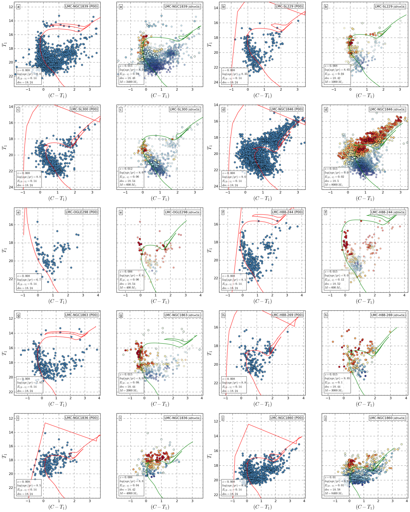
Figure 21: CMDs for the P00 database.

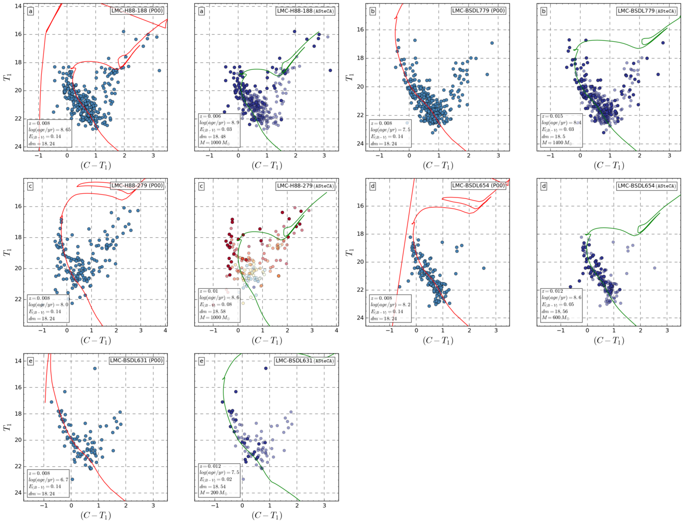
Figure 22: CMDs for the P00 database.

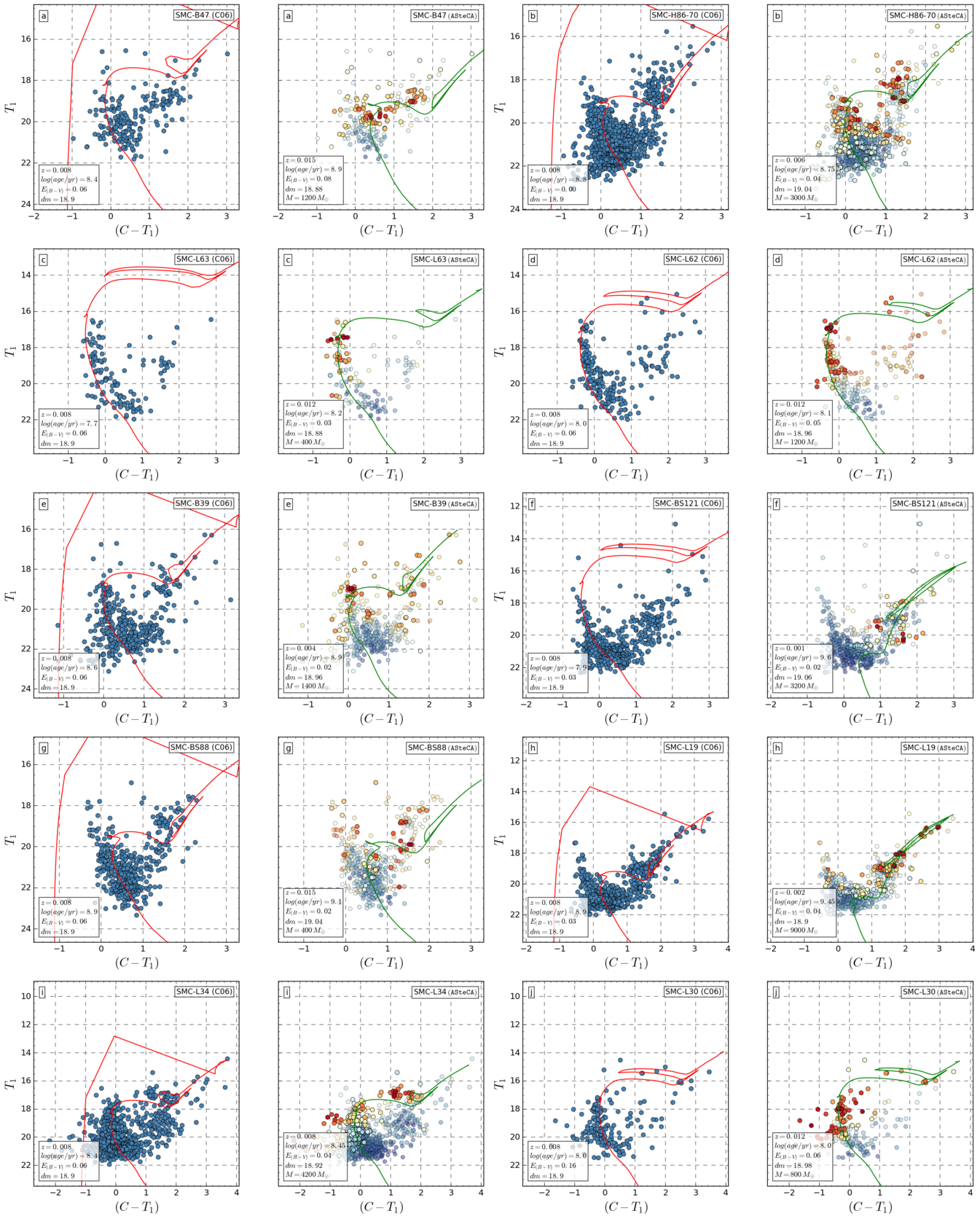
Figure 23: CMDs for the C06 database.

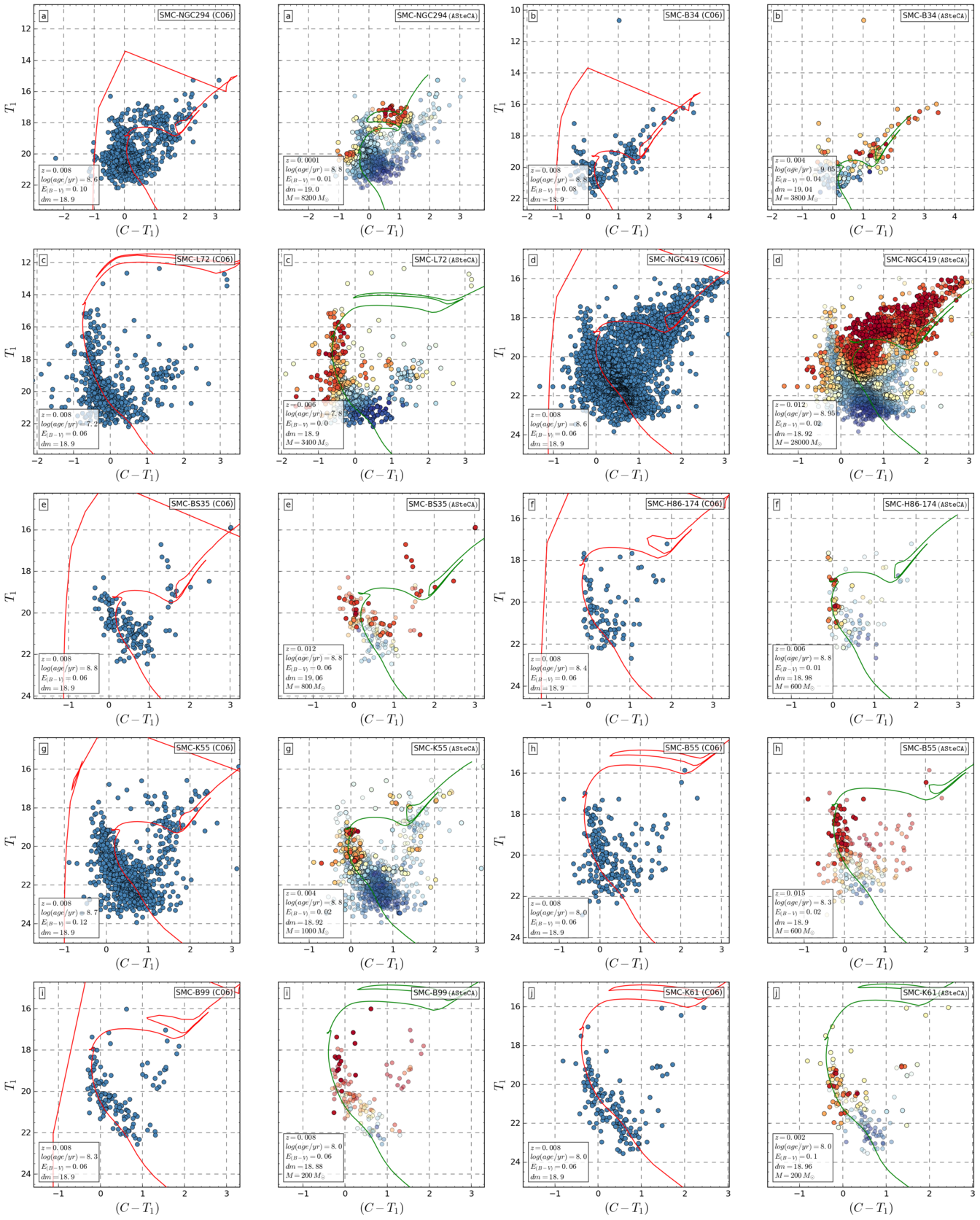
Figure 24: CMDs for the C06 database.

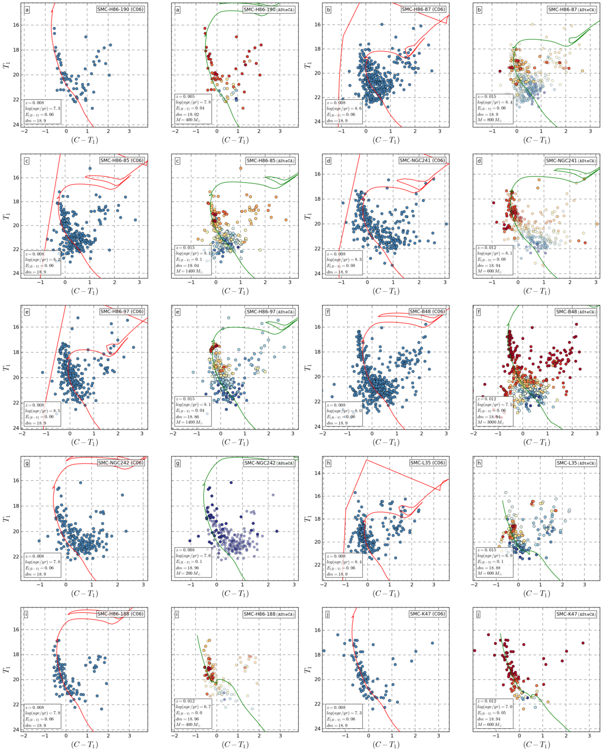
Figure 25: CMDs for the C06 database.

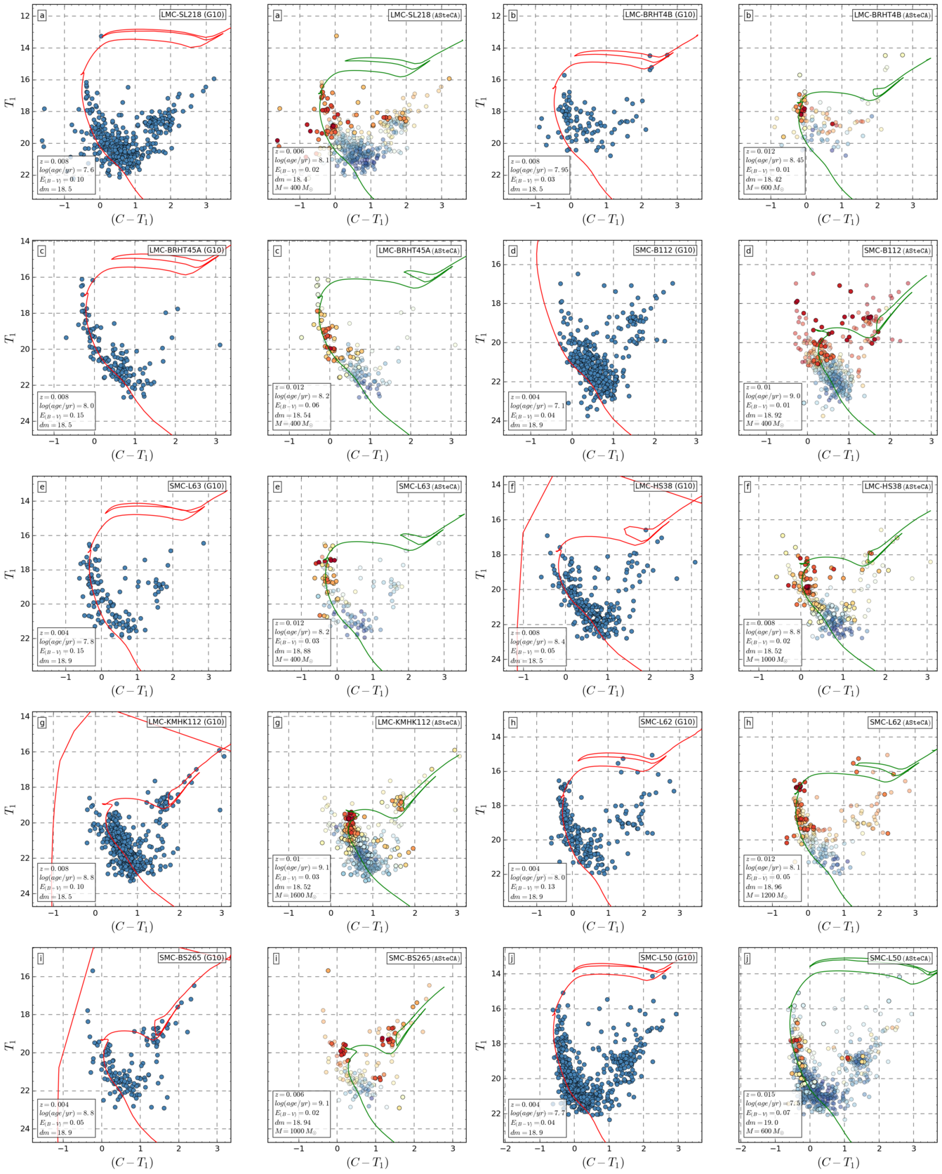
Figure 27: CMDs for the G10 database.

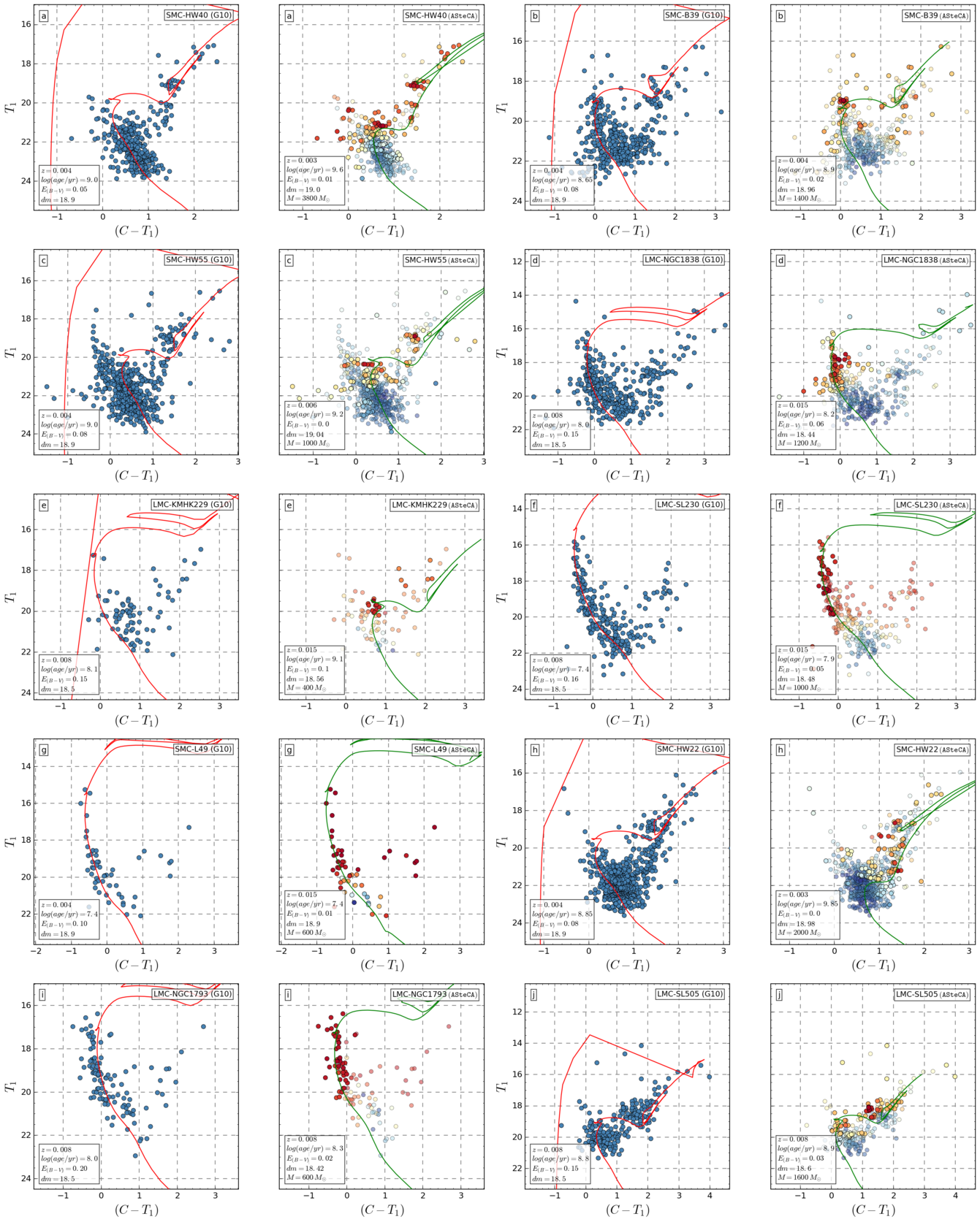
Figure 28: CMDs for the G10 database.

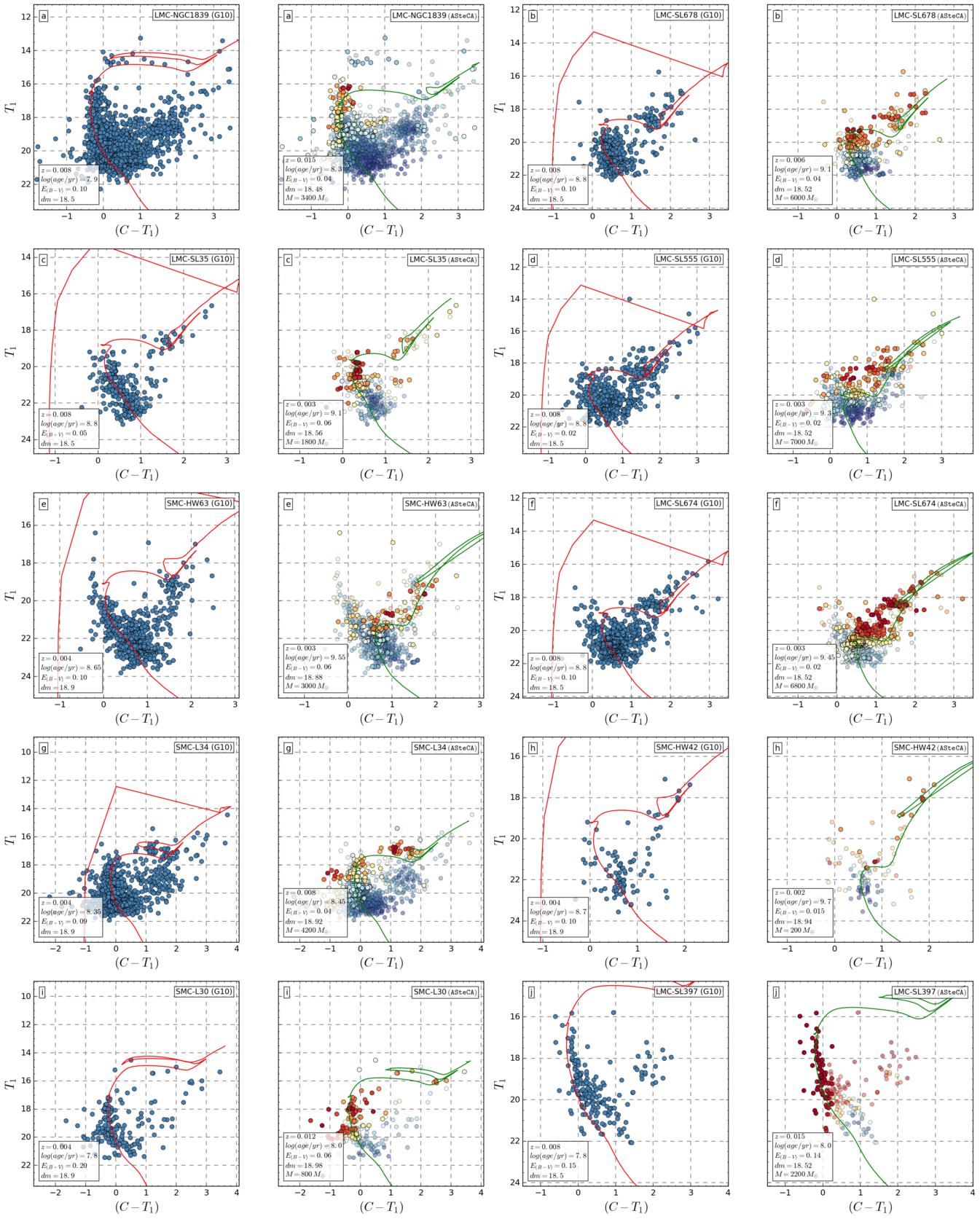
Figure 29: CMDs for the G10 database.

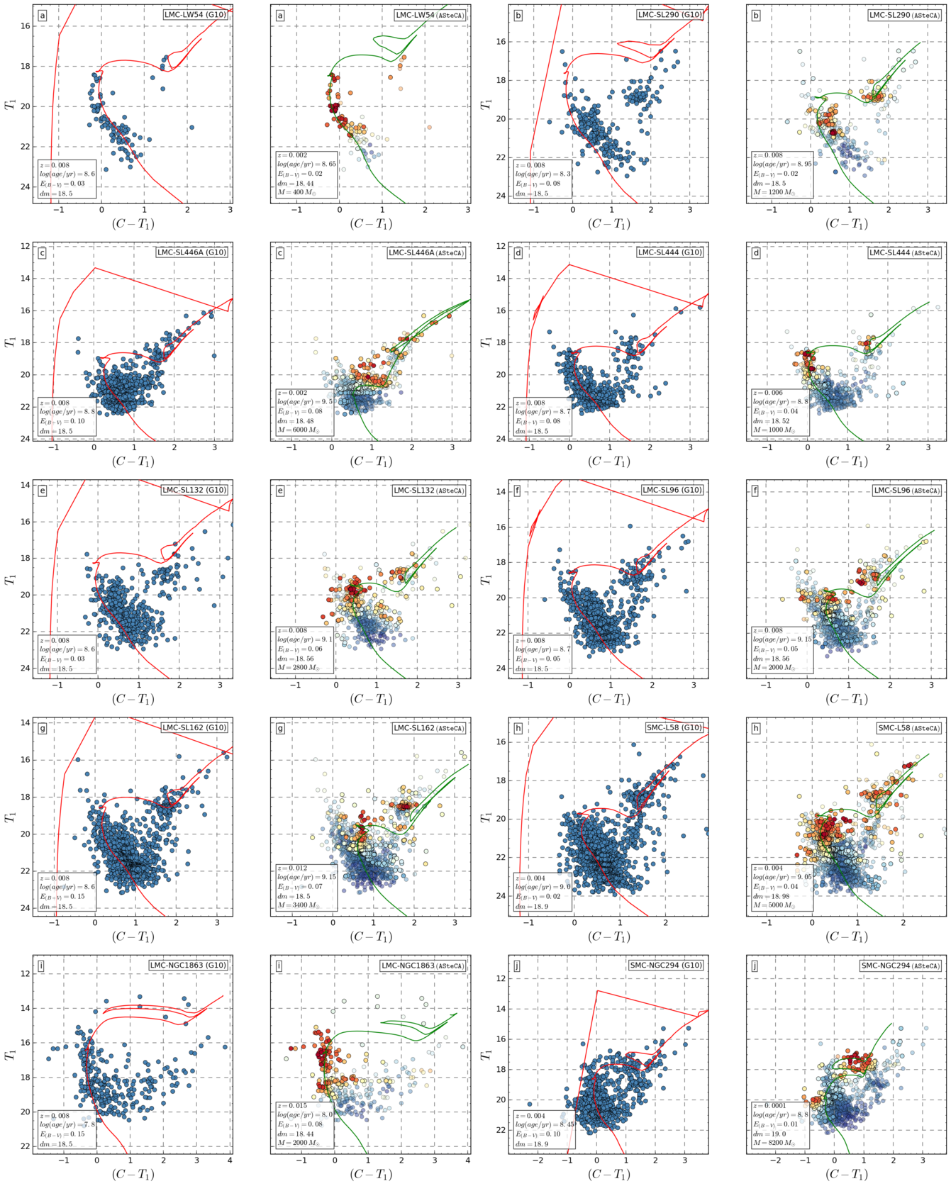
Figure 30: CMDs for the G10 database.

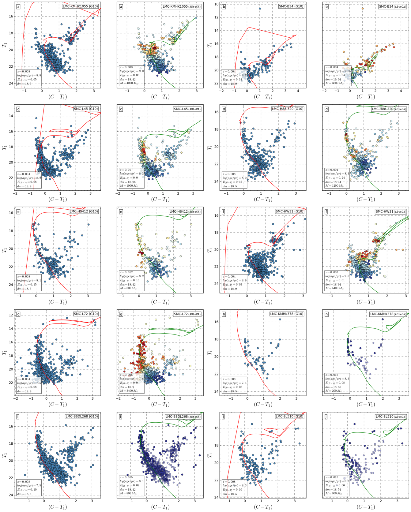
Figure 31: CMDs for the G10 database.

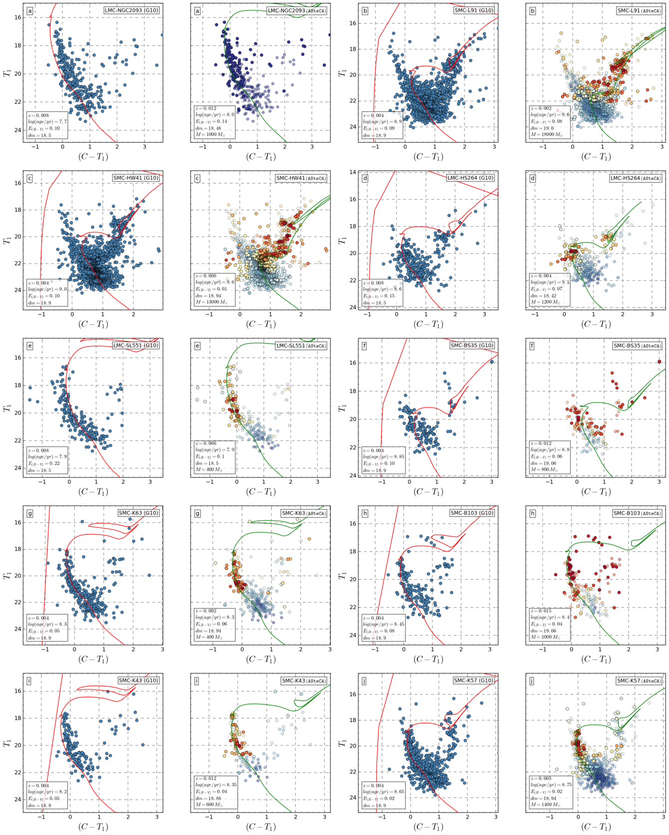
Figure 32: CMDs for the G10 database.

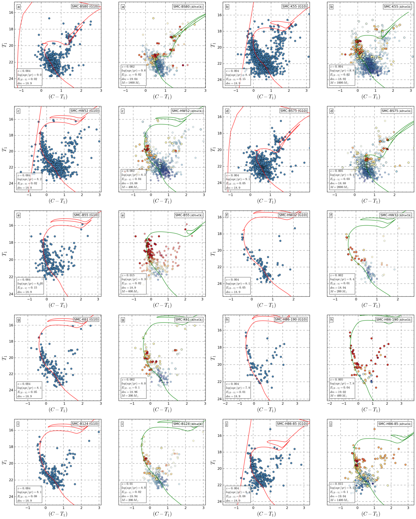
Figure 33: CMDs for the G10 database.

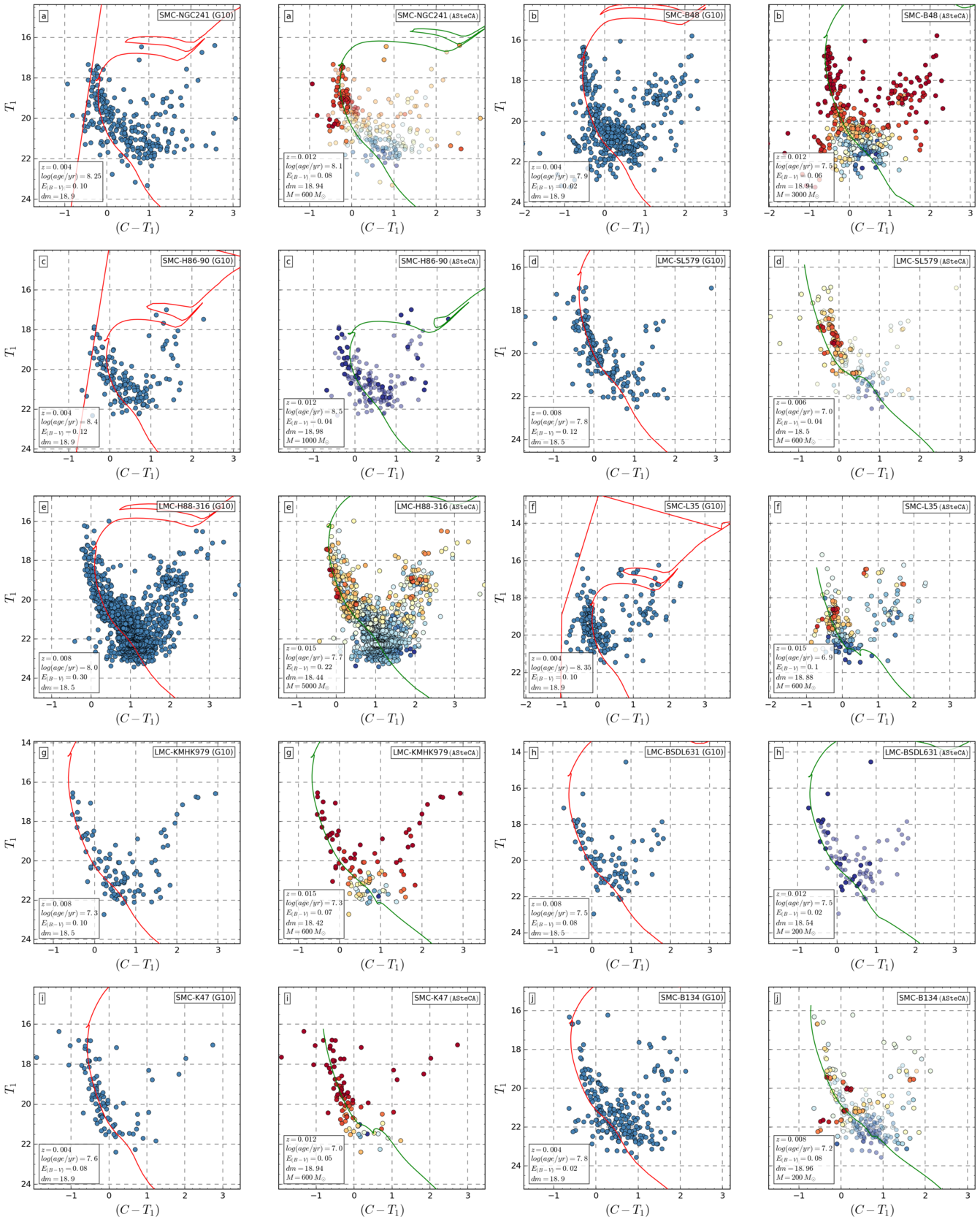
Figure 34: CMDs for the G10 database.

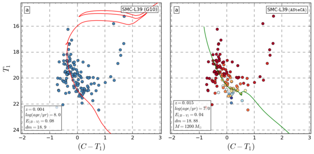
Figure 35: CMDs for the G10 database.

Appendix D Mathematical description of the age-metallicity relationship

We use the KDE technique described in Sect. 6 to generate an AMR representative of the observed data, with some important improvements over previous methods. First, unlike a regular histogram, a Gaussian density map has no dependence on the number, size (fixed or variable) or location of bins. Second, the errors in the two parameters used to obtain the density map (age and metallicity), are organically included in the function that generates it (as explained in Sect. 6). No ad-hoc procedure is needed to incorporate the information carried by these values, into the final AMR.

The process of creating an AMR function requires assigning a unique [Fe/H] to a single age value, for the available age range. A dense grid is created to divide the age-metallicity 2D density map into N steps of 0.01 dex width, covering the ranges of both parameters. Every point in this grid is evaluated in the KDE map and its value ($w_{i}$) is stored, along with its age-metallicity coordinates ($age_{i},\;[\mathrm{Fe/H}]_{i}$). The N ages in the grid are then associated to N single representative [Fe/H] values, obtained as the mean metallicity value weighted by the KDE function at that particular age. The formal equation can be written as

$$\overline{[Fe/H]}_{age_{i}}=\frac{\sum w_{i}{[Fe/H]}_{i}}{\sum w_{i}}$$ (6)

where the summations are performed over the N steps in the metallicity range, ${[Fe/H]}_{i}$ is the metallicity value at step $i$, and $w_{i}$ is the value of the 2D KDE map for that fixed age and metallicity coordinates. The $age_{i}$ subindex in Eq. 6 indicates that this mean metallicity was calculated for a fixed age value, and thus represents a unique point in the AMR. A similar version of this method was employed in Noël et al. (2009, see Eq. 3) to derive AMR estimates for three observed fields. We apply the above formula to all ages in the grid defined at the beginning of the process. The standard deviation for each $\overline{[Fe/H]}_{age_{i}}$ value is calculated as

$$\sigma_{age_{i}}^{2}=\frac{\sum w_{i}\sum[w_{i}{({[Fe/H]}_{i}-\overline{[Fe/H]}_{age_{i}})}^{2}]}{{(\sum w_{i})}^{2}-\sum w_{i}^{2}}$$ (7)

where again all summations are applied over N, and the descriptions given for the parameters in Eq. 6 apply. At this point, this method already gives us an AMR function estimate, since every age step is mapped to a unique metallicity. The downsides are that the AMR is noisy due to the very small step of 0.01 dex used, and the associated errors are quite large. This latter effect arises because the weighted standard deviation, Eq. 7, is affected not only by errors in both measured parameters but also by the intrinsic dispersion in the metallicity values found for any given age. We therefore calculate the average [Fe/H] for an age interval, rather than assigning a metallicity value to each age step in the grid. Dividing the age range into intervals requires a decision about the step width, much like when constructing a histogram, bringing back the issue of binning. We have two advantages here: a) we use Knuth’s algorithm (see Sect. 3.4) to obtain the optimal binning for our data, and b) the final AMR function is very robust to changes in the binning method selected, so even the previous choice is not crucial in determining the shape of our AMR. Finally, the $\overline{[Fe/H]}_{age_{i}}$ values obtained for every ${age_{i}}$ within a defined age interval, are averaged. Errors are propagated through the standard formula, disregarding covariant terms (Bevington & Robinson 2003, Eq. 3.14).

In Fig. 36 we show the AMRs for both Clouds, generated using metallicity and age values taken from the “literature” articles, see Table. 1. Most clusters in these works are assigned fixed metallicities of -0.7 dex (SMC) and -0.4 dex (LMC), particularly for estimated ages below 1 Gyr. This explains the average difference of ${\sim}0.2$ dex that can be appreciated, when compared to ASteCA’s AMRs (Fig. 13).

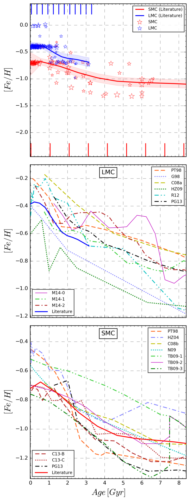
Figure 36: Age-metallicity relationships for our set of 239 clusters, using $\log\mathrm{(age/yr)}$ and [Fe/H] values taken from the literature.