Coarse graining the phase space of $N$ qubits

Abstract

We develop a systematic coarse graining procedure for systems of $N$ qubits. We exploit the underlying geometrical structures of the associated discrete phase space to produce a coarse-grained version with reduced effective size. Our coarse-grained spaces inherit key properties of the original ones. In particular, our procedure naturally yields a subset of the original measurement operators, which can be used to construct a coarse discrete Wigner function. These operators also constitute a systematic choice of incomplete measurements for the tomographer wishing to probe an intractably large system.

I Introduction

Recently, the understanding of many-body quantum systems has dramatically progressed. Nowadays we are achieving an amazing degree of control over larger and larger systems Bloch et al. (2008); Blatt and Roos (2012). Therefore, verification during each stage of experimental procedures is of utmost importance; quantum tomography is the appropriate tool for that purpose.

The goal of quantum tomography is to reconstruct the state of a system by performing multiple measurements on identically prepared copies of the system. Once the experimental data are extracted, a numerical procedure determines which density matrix fits best the measurements. This estimation can be performed using different approaches, such as maximum likelihood estimation Paris and Řeháček (2004), or Bayesian methods Bužek et al. (1998); Schack et al. (2001); Huszár and Houlsby (2012); Granade et al. (2016). However, tomography becomes harder as we explore more intricate systems. If we look at the simple, yet illustrative case of $N$ qubits, which will serve as the consistent thread in this paper, one has to make at least $2^{N}+1$ measurements in different bases before one can claim to know everything about an a priori unknown system. With such an exponential scaling in the number of qubits, it is clear that current methods rapidly become intractable for present state-of-the-art experiments.

As a result, more sophisticated tomographical techniques are called for. New protocols try to simplify the process by making an educated guess about the nature of the state. Among other assumptions, this includes rank deficiency Gross et al. (2010); Cramer et al. (2010); Flammia et al. (2012); Landon-Cardinal and Poulin (2012); Baumgratz et al. (2013), extra symmetries Tóth et al. (2010); Moroder et al. (2012); Klimov et al. (2013), or Gaussianity Řeháček et al. (2009). While all these approaches are extremely efficient, their pitfall is that when the starting guess is inaccurate, they produce significant systematic errors.

Here, we pursue a different approach, inspired by a notion from statistical mechanics: coarse graining Castiglione et al. (2008). This operation transforms a probability density in phase space into a “coarse-grained” density that is a piecewise constant function, a result of density averaging in cells. This is the chief idea behind the renormalization group White (1992), which allows a systematic investigation of the changes of a physical system as viewed at different scales.

In our case, we consider a system of qubits and look at the associated phase space, which turns out to be a discrete grid of $2^{N}\times 2^{N}$ points. We assign to each suitably defined line in phase space a specific rank-one projection operator representing a pure quantum state. For each point of the grid, a suitable quasi-probability as the Wigner function can be directly computed from the measurement of the states associated with the lines passing through that point. We coarse grain by combining groups of these lines into thick lines, which we will show to be lines in the phase space of an effectively smaller system. Our coarse-grained phase spaces are endowed with many nice properties.

Most notably, our procedure systematically and naturally reveals a subset of measurements which one could use to perform incomplete tomography. In addition, using the coarse-grained points and lines, we show that one can define a discrete Wigner function in largely the same way as it is defined in the original space. When plotted, the coarse functions resemble smoothed out versions of the originals, preserving many of their prominent visual features.

II Phase space of $N$ qubits

A qubit is a two-dimensional quantum system, with Hilbert space isomorphic to $\mathbb{C}^{2}$. It is customary to choose two normalized orthogonal states, say $\{|0\rangle,|1\rangle\}$, as a computational basis. The unitary matrices

$$\sigma_{z}=|0\rangle\langle 0|-|1\rangle\langle 1|\,,\qquad\qquad\sigma_{x}=|0\rangle\langle 1|+|1\rangle\langle 0|\,,$$ (1)

generate the Pauli group $\mathcal{P}_{1}$, which consists of all the Pauli matrices plus the identity, with multiplicative factors $\pm 1,\pm i$ Chuang and Nielsen (2000).

For $N$ qubits, the corresponding Hilbert space is the tensor product $\mathbb{C}^{2}\otimes\cdots\otimes\mathbb{C}^{2}=\mathbb{C}^{2^{N}}$. A compact way of labeling both states and elements of the corresponding Pauli group $\mathcal{P}_{N}$ is by using the finite field $\mathbb{F}_{2^{N}}$. In Appendix A we briefly summarize the basic notions of finite fields needed to proceed.

Let $|\nu\rangle$, $\nu\in\mathbb{F}_{2^{N}}$, be an orthonormal basis in the Hilbert space $\mathbb{C}^{2^{N}}$ (henceforth, field elements will be denoted by Greek letters). The elements of the basis can be labeled by powers of a primitive element $\sigma$ (i.e., a root of an irreducible primitive polynomial): $\{|0\rangle,\,|\sigma\rangle,\ldots,\,|\sigma^{2^{N}-1}=1\rangle\}$. Now the equivalent version of (1) is Grassl et al. (2003); Vourdas (2004, 2007)

$$Z_{\alpha}=\sum_{\nu}\chi(\alpha\nu)\,|\nu\rangle\langle\nu|\,,\qquad X_{\beta}=\sum_{\nu}|\nu+\beta\rangle\langle\nu|\,,$$ (2)

so that

$$Z_{\alpha}X_{\beta}=\chi(\alpha\beta)\,X_{\beta}Z_{\alpha}\,,$$ (3)

which is the discrete counterpart of the Weyl-Heisenberg algebra for continuous variables Binz and Pods (2008). Here, the additive character $\chi$ is defined as $\chi(\alpha)=\exp[i\pi\mathop{\mathrm{tr}}\nolimits(\alpha)]$ and the trace of a field element (we distinguish it from the trace of an operator by the lower case “tr”) is defined in Appendix A. Moreover, $Z_{\alpha}$ and $X_{\beta}$ are related through the finite Fourier transform Klimov et al. (2005)

$$\mathcal{F}=\frac{1}{\sqrt{2^{N}}}\sum_{\nu,\nu^{\prime}}\chi(\nu\,\nu^{\prime})\,|\nu\rangle\langle\nu^{\prime}|\,,$$ (4)

so that $X_{\alpha}=\mathcal{F}\,Z_{\alpha}\,\mathcal{F}^{\dagger}$.

The operators (2) generate the Pauli group $\mathcal{P}_{N}$ of $N$ qubits and, with a suitable choice of basis, they can be factorized into a tensor product of single-qubit Pauli operators. To this end, it is convenient to consider $\mathbb{F}_{2^{N}}$ as an $N$-dimensional linear space over $\mathbb{Z}_{2}$. It is spanned by an abstract basis $\{\theta_{1},\ldots,\theta_{N}\}$, so that given a field element $\alpha$ the expansion

$$\alpha=\sum_{i=1}^{N}a_{i}\,\theta_{i}\,,\qquad a_{i}\in\mathbb{Z}_{2}\,,$$ (5)

allows us the identification $\alpha\Leftrightarrow(a_{1},\ldots,a_{N})$. The basis $\{\theta_{i}\}$ can be chosen to be orthonormal with respect to the trace operation; i.e., $\mathop{\mathrm{tr}}\nolimits(\theta_{i}\,\theta_{j})=\delta_{ij}$. This is a self-dual basis, which always exist for the case of qubits. In this way, we associate each qubit with a particular element of the self-dual basis: qubit${}_{i}\Leftrightarrow\theta_{i}$. Using this basis, we have the factorization

$$Z_{\alpha}=\sigma_{z}^{a_{1}}\otimes\cdots\otimes\sigma_{z}^{a_{N}},\qquad X_{\beta}=\sigma_{x}^{b_{1}}\otimes\cdots\otimes\sigma_{x}^{b_{N}}\,,$$ (6)

where $a_{i}=\mathop{\mathrm{tr}}\nolimits(\alpha\theta_{i})$ and $b_{i}=\mathop{\mathrm{tr}}\nolimits(\beta\theta_{i})$ are the corresponding expansion coefficients for $\alpha$ and $\beta$ in the self-dual basis.

We next recall Wootters (2004); Gibbons et al. (2004) that the grid defining the phase space for $N$ qubits can be appropriately labeled by the discrete points $(\alpha,\beta)$, which are precisely the indices of the operators $Z_{\alpha}$ and $X_{\beta}$: $\alpha$ is the “horizontal” axis and $\beta$ the “vertical” one. In this grid we can introduce the set of displacements

$$D(\alpha,\beta)=\Phi(\alpha,\beta)\,Z_{\alpha}X_{\beta}\,,$$ (7)

where $\Phi(\alpha,\beta)$ is a phase required to avoid plugging extra factors when acting with $D$. A sensible choice for the case of qubits is $\Phi^{2}(\alpha,\beta)=\chi(\alpha\beta)$, which ensures the Hermiticity of the displacement operators. In addition, we impose $\Phi(\alpha,0)=1$ and $\Phi(0,\beta)=1$, which means that the displacements along the “position” axis $\alpha$ and the “momentum” axis $\beta$ are not associated with any phase. These displacement operators shift phase space points, so the action of $D(\alpha^{\prime},\beta^{\prime})$ maps $(\alpha,\beta){\mapsto}(\alpha+\alpha^{\prime},\beta+\beta^{\prime})$, justifying their designation. Note that we still have to fix the sign of the phase $\Phi(\alpha,\beta)$. We choose the phase as

$$\Phi(\alpha,\beta)=i^{\mathop{\mathrm{tr}}\nolimits(\alpha\beta)}(-1)^{f(\alpha\beta)}\,,$$ (8)

where $f(x)=\sum_{0\leq j<i\leq m-1}x^{2^{i}+2^{j}}$, which ensures that the operators defined in Eq. (17) below are rank-one projections.

On the phase space grid one can introduce a variety of geometrical structures with much the same properties as in the continuous case Klimov et al. (2007, 2009); Muñoz et al. (2012). The simplest are the straight lines passing through the origin (also called rays), with equations

$$\alpha=0,\qquad\mathrm{or}\qquad\beta=\lambda\alpha\,.$$ (9)

The rays have a very remarkable property: the monomials $D(\alpha,\beta)$ belonging to the same ray commute, and thus, have a common system of eigenvectors $\{|\psi_{\nu,\lambda}\rangle\}$,

$$D(\alpha,\lambda\alpha)|\psi_{\nu,\lambda}\rangle=\exp(i\xi_{\nu,\lambda})|\psi_{\nu,\lambda}\rangle,$$ (10)

where $\lambda$ is fixed and $\exp(i\xi_{\nu,\lambda})$ is the corresponding eigenvalue, so $|\psi_{\nu,0}\rangle=|\nu\rangle$ are eigenstates of $Z_{\alpha}$ (displacement operators labeled by the ray $\beta=0$, which we take as the horizontal axis). The projection operators associated with the lines of equal slope are the projections onto these eigenvactors. Indeed, we have that

$$|\langle\psi_{\nu,\lambda}|\psi_{\nu^{\prime},\lambda^{\prime}}\rangle|^{2}=\delta_{\lambda,\lambda^{\prime}}\delta_{\nu,\nu^{\prime}}+\frac{1}{2^{N}}(1-\delta_{\lambda,\lambda^{\prime}}),$$ (11)

and, in consequence, they are mutually unbiased bases (MUBs) Wootters and Fields (1989).

Now suppose for each ray we disregard the origin $(0,0)$, whose monomial is the identity operator. This leaves us with $2^{N}-1$ commuting operators. If we then consider the whole bundle of $2^{N}+1$ rays (which are obtained by varying the “slope” $\lambda$ over all of $\mathbb{F}_{2^{N}}$), we can construct a complete set of MUB operators arranged in a $(2^{N}-1)\times(2^{N}+1)$ table Bandyopadhyay et al. (2002).

To round up the scenario, we need to represent states in phase space. The discrete Wigner function Björk et al. (2008) is the appropriate tool. It can be considered as an invertible mapping

$$W_{\varrho}(\alpha,\beta)=\frac{1}{2^{N}}\mathop{\mathrm{Tr}}\nolimits[\varrho\,\Delta(\alpha,\beta)]\,,$$ (12)

so that

$$\varrho=\sum_{\alpha,\beta}\Delta(\alpha,\beta)\,W_{\varrho}(\alpha,\beta)\,.$$ (13)

The operational kernel is defined as

$$\Delta(\alpha,\beta)=\frac{1}{2^{N}}\sum_{\alpha^{\prime},\beta^{\prime}}\chi(\alpha\alpha^{\prime}-\beta\beta^{\prime})\,D(\alpha^{\prime},\beta^{\prime})\,,$$ (14)

which, in view of equation (4), can be interpreted as a double Fourier transform of $D(\alpha,\beta)$. One can check that this kernel has all the good properties Stratonovich (1956): it is Hermitian, normalized and covariant under the Pauli group. As a result, for each point on the grid, the corresponding value of the Wigner function can be computed from the probabilities of measuring the pure states associated with the lines passing through that point.

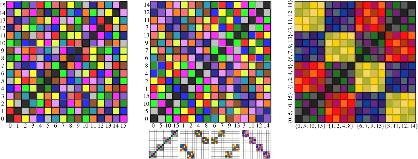
Figure 1: Graphical sketch of coarse graining. Here we consider dimension 16, and its diagonal ray, $\beta=\alpha$. The first panel plots all the lines of the form $\beta=\alpha+\gamma$, parametrized by the shift $\gamma$. Points on the same line have the same colour. Axis labels correspond to powers of the primitive element of $\mathbb{F}_{16}$, with the convention that $\sigma^{0}$ is denoted by 0 and $\sigma^{15}=1$. The middle panel shows the original grid with the axis labels permuted such that coset elements are grouped together. We can see that this leads to distinct $4\times 4$ blocks containing points of exactly four different colours. These are shown expanded out in the small, lower four grids. One notices that these “coarse” blocks form the diagonal ray and all its translates in dimension $4$, which we show superimposed in the last panel.

III Coarse graining

As heralded in the Introduction, our goal is to tailor a procedure that allows us to coarse grain the phase space of a multiqubit system; i.e., to break it down into simpler sub-components.

To this end, we consider the number $N$ of qubits to be composite, i.e. $N=mn$. Let $\{\mu_{0},\ldots,\mu_{n-1}\}$ be a basis of $\mathbb{F}_{2^{mn}}$ with respect to $\mathbb{F}_{2^{m}}$. We define

$$\mathfrak{C}_{0}=\left\{\sum_{j=1}^{n-1}\tau_{j}\mu_{j}\enskip|\enskip\tau_{j}\in\mathbb{F}_{2^{m}}\right\}\,,$$ (15)

i.e., the subspace made of linear combinations of basis elements $\mu_{1},\ldots,\mu_{n-1}$ with coefficients in the base field $\mathbb{F}_{2^{m}}$. We can use this set $\mathfrak{C}_{0}$, which we henceforth refer to as the initial coset, to decompose the field $\mathbb{F}_{2^{mn}}$ into cosets:

$$\mathfrak{C}_{\tau}=\tau\mu_{0}+\mathfrak{C}_{0},\qquad\tau\in\mathbb{F}_{2^{m}}\,.$$ (16)

The coarse-grained space will be labeled according to these cosets.

We can imagine the process of coarse graining as partitioning the grid $\mathbb{F}_{2^{mn}}\times\mathbb{F}_{2^{mn}}$ in such a way that we superimpose a grid of size $2^{m}\times 2^{m}$ on top, with each superimposed point indexed by cosets rather than field elements in the original grid. Each point in the coarse grid then contains a sub-grid the same size as $\mathbb{F}_{2^{m}}^{n-1}\times\mathbb{F}_{2^{m}}^{n-1}$. To provide some intuition for this, we show a visual example of this process in action in Fig. 1.

Our procedure for coarse-graining the grid arises naturally from consideration of the line structure of phase space. We will use the thin lines in $\mathbb{F}_{2^{mn}}$ to create thick lines in the coarse phase space, by grouping together lines having the same slope, and with intercepts in the same coset. We write thin lines in the big field $\mathbb{F}_{2^{mn}}$ as $|\ell^{(\lambda)}_{\gamma}\rangle$, where $\lambda$ is the slope, and $\gamma$ is the intercept. A large, coarse-grained line is denoted as $|L^{(\lambda)}_{\mathfrak{C}_{\tau}}\rangle$, where now the intercept is a whole coset.

To each line in the fine-grained phase space we can assign a projector $|\ell^{(\lambda)}_{\gamma}\rangle\langle\ell^{(\lambda)}_{\gamma}|$, constructed as a linear combination of the displacement operators. We choose as our convention for the rays $(\gamma=0)$ the all-positive sum

$$|\ell^{(\lambda)}_{0}\rangle\langle\ell^{(\lambda)}_{0}|=\frac{1}{2^{mn}}\sum_{\alpha}D(\alpha,\lambda\alpha).$$ (17)

These lines are eigenstates with eigenvalue $+1$ for all displacement operators in the sum. Projectors with nonzero intercepts are obtained by conjugating that of the ray with an appropriate displacement operator.

The coarse lines are produced by grouping together lines with intercepts in the same coset:

$$|L^{(\lambda)}_{\mathfrak{C}_{\tau}}\rangle\langle L^{(\lambda)}_{\mathfrak{C}_{\tau}}|=\sum_{\gamma\in\mathfrak{C}_{\tau}}|\ell^{(\lambda)}_{\gamma}\rangle\langle\ell^{(\lambda)}_{\gamma}|\,.$$ (18)

The possible choices of slope for these lines will be limited to elements of the subfield $\mathbb{F}_{2^{m}}$, as these have natural analogues between the two fields.

As discussed in more detail in Appendix B, the coarse rays of Eq. (18) can be simplified and rewritten as the sum of displacement operators

$$|{L}^{(\lambda)}_{\mathfrak{C}_{0}}\rangle\langle{L}^{(\lambda)}_{\mathfrak{C}_{0}}|=\frac{1}{2^{mn}}\sum_{\lambda}\left[\sum_{\gamma\in\mathfrak{C}_{0}}\chi(\gamma\alpha)\right]D(\alpha,\lambda\alpha)\,.$$ (19)

One can check here that the inner sum over the elements of $\mathfrak{C}_{0}$ will cause some of the displacement operators to vanish. The sum in brackets in Eq. (19) is either zero or a positive constant. Hence, the projection associated to the thick lines are a sum over a subset of the displacement operators associated with the thin lines. This leads us to the key idea of our work: rather than measuring all the displacement operators, we measure only those which are present in the rays of the coarse-grained space.

We note here that the choice of $\mathfrak{C}_{0}$ is not unique, and will ultimately determine the resultant set of displacement operators. For example, a special case occurs when the dimension of the system is square. In this case, we can consider the relationship between the fields as a quadratic field extension, i.e. when $n=2$. In this case we can partition $\mathbb{F}_{2^{2m}}$ into $\mathbb{F}_{2^{m}}\times\mathbb{F}_{2^{m}}$. We can then choose the initial coset as the copy of the subfield $\mathbb{F}_{2^{m}}\subset\mathbb{F}_{2^{2m}}$:

$$\mathfrak{C}_{0}=\{\sigma^{i\left(2^{m}+1\right)},\enskip i=0,\ldots,2^{m}-1\}\,,$$ (20)

where $\sigma$ is a primitive element of $\mathbb{F}_{2^{mn}}$ and we use the notation $\sigma^{0}$ for 0. The subsequent cosets are obtained additively from this subfield using the representatives $\tau_{i}=\sigma^{2^{m}\left(i-1\right)+i}$.

Finally, the coarse-grained phase space inherits a coarse-grained Wigner function. A coarse kernel can be constructed by grouping together kernel operators from the same coset, i.e.

$$\mathfrak{D}(\mathfrak{C}_{\tau},\mathfrak{C}_{\xi})=\sum_{\alpha\in\mathfrak{C}_{\tau}}\sum_{\beta\in\mathfrak{C}_{\xi}}\Delta(\alpha,\beta)\,.$$ (21)

Desired properties of a Wigner function all follow from the original kernel. As was the case with the displacement operators, differing choices of the subset $\mathfrak{C}_{0}$ will lead to differing Wigner functions.

IV Examples

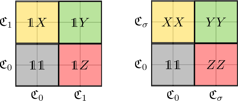
Figure 2: Resultant operators from coarse-graining a dimension 4 system down to dimension $2$. Colours are indicative of particular coarse rays. The left image coarse grains by taking $\mathfrak{C}_{0}=\{0,\sigma\}$, whereas the lower image uses the subfield $\mathfrak{C}_{0}=\{0,1\}$.

We illustrate the previous ideas with some relevant examples. We have written a Python software package capable of generating all the following results, which we make available online Bal

The first nontrivial instance we can have is the case of two qubits, so dimension $4$. Using the irreducible primitive polynomial $x^{2}+x+1=0$, we have that $\mathbb{F}_{4}=\{0,1,\sigma,\sigma^{2}=\sigma+1\}$. The self-dual basis is $\{\sigma,\sigma+1\}$, and we use it to produce the displacement operators.

Another basis for $\mathbb{F}_{4}/\mathbb{F}_{2}$ is $\{1,\sigma\}$. Taking all scalar multiples of $\mu_{1}=\sigma$ from the prime field gives us $\mathfrak{C}_{0}=\{0,\sigma\}$. We then obtain $\mathfrak{C}_{1}=1+\mathfrak{C}_{0}=\{1,\sigma^{2}\}$. For each ray, we can list the operators which survive in the inner sum over $\mathfrak{C}_{0}$ in Eq. (19). Moreover, we can label the points of the coarse-grained grids by those displacement operators. Disregarding the identity operator, the resulting set $\{\openone X,\openone Z,\openone Y\}$ constitutes the appropriate measurements to be performed to determine which coarse-grained line they are in. They are essentially Pauli measurements on one of the two qubits in the system.

Alternatively, the dimension is a square, so we can choose as our initial coset the subfield $\mathbb{F}_{2}$: $\mathfrak{C}_{0}=\{0,1\}$. This yields the second coset $\mathfrak{C}_{\sigma}=\{\sigma,\sigma^{2}\}$. We once again compute the surviving operators using Eq. (19). The final result now is $\{XX,YY,ZZ\}$. Here, we see that we are making a measurement with the same Pauli operator on both qubits, thereby capturing the full correlations between the two qubits. Figure 2 shows both partitioning methods side by side.

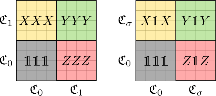
Figure 3: Resultant operators from coarse-graining a dimension $8$ system down to dimension $2$. (Left panel) Coarse graining using the basis $\{1,\sigma,\sigma^{2}\}$. The resultant measurements are unitarily equivalent to a case where two of the qubits remain untouched. (Right panel) Resultant operators when the coarse-graining uses the initial basis $\{\sigma,\sigma^{4},\sigma^{5}\}$. Here we obtain the interesting result that all resultant operators commute.

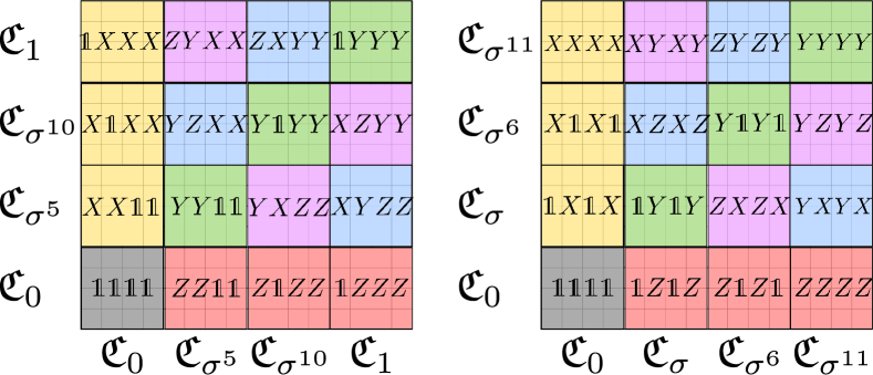
Figure 4: Resultant operators from coarse-graining a dimension $16$ system down to dimension $4$. The left panel contains the surviving operators from the general basis method, the right panel from choosing the subfield as $\mathfrak{C}_{0}$. The cosets are listed in Eqs. (25) and (26) respectively. In the case of the left panel, these operators are unitarily equivalent to a set where two qubits are untouched and the 2-qubit MUB operators are applied to the rest. The right panel has no such transformation.

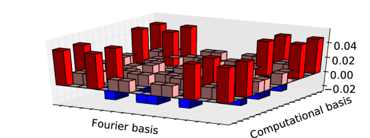
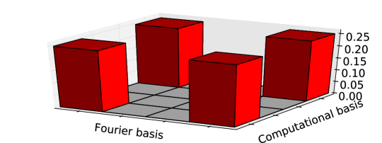
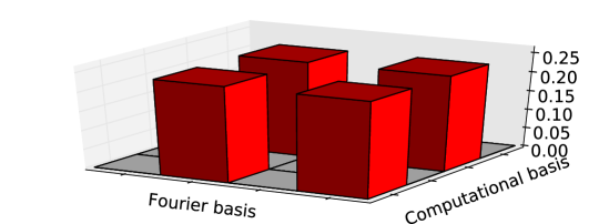
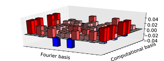
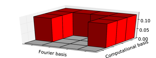
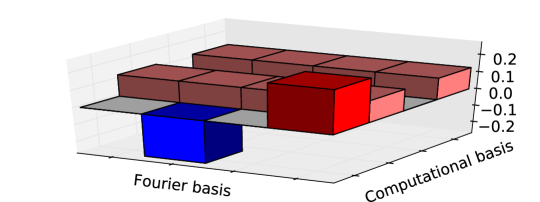
Figure 5: (Top) Coarse-grained Wigner function for the state $\frac{1}{2}(|00\rangle+|11\rangle)\otimes(|00\rangle+|11\rangle)$. (Left) The original Wigner function in dimension 16. The $x$-axis represents the computational basis, in the standard ordering $|0000\rangle,|0001\rangle,|0010\rangle$, etc. The Fourier basis, as defined via Eq. (4), is on the $y$-axis and is similarly ordered. (Centre) Coarse graining over $\mathbb{F}_{4}$ with the polynomial basis $\{1,\sigma\}$. Here the axes are not labeled by single states, but rather by a set of states associated with each coset. (Right) Coarse graining with the subfield as the initial coset. (Bottom) The same coarse graining procedure as above, but applied to the state $\frac{1}{2}(|0001\rangle+|0010\rangle+|0100\rangle+|1000\rangle)$.

Our next example is the case of dimension 8. We choose $\sigma$ a root of the irreducible primitive polynomial $x^{3}+x+1=0$, and obtain a self-dual basis $\{\sigma^{3},\sigma^{5},\sigma^{6}\}$. An obvious choice for a basis of $\mathbb{F}_{8}/\mathbb{F}_{2}$ is a polynomial basis $\{1,\sigma,\sigma^{2}\}$. To construct $\mathfrak{C}_{0}$, we must take all possible linear combinations of $\sigma$ and $\sigma^{2}$ with coefficients in $\mathbb{F}_{2}$. This produces

$$\mathfrak{C}_{0}=\{0,\sigma,\sigma^{2},\sigma^{4}\}.$$ (22)

We obtain the second coset by adding the remaining subfield element $1$ to $\mathfrak{C}_{0}$:

$$\mathfrak{C}_{1}=\{1,\sigma^{3},\sigma^{5},\sigma^{6}\}.$$ (23)

The traces of all elements in $\mathfrak{C}_{0}$ are $0$, and the traces for all elements in $\mathfrak{C}_{1}$ are $1$. The surviving four operators are shown in Fig. 3.

Using a Clifford transformation, we can “trace out” two of the qubits. The sequence of CNOT gates: CNOT₁₂ – CNOT₁₃ – CNOT₂₁ – CNOT₃₁ transforms the set into $\{X\openone\openone,Z\openone\openone,Y\openone\openone\}$, so we see that this partitioning is, after a global change of basis, equivalent to measuring each Pauli on only a single qubit.

If we choose instead the basis $\{\sigma,\sigma^{4},\sigma^{5}\}$ to build our cosets, we get a more interesting result:

$$\mathfrak{C}_{0}=\{0,1,\sigma^{4},\sigma^{5}\},\qquad\mathfrak{C}_{\sigma}=\{\sigma,\sigma^{2},\sigma^{3},\sigma^{6}\}.$$ (24)

The operators that survive have the form $Z_{\alpha}X_{\beta}$, $\alpha,\beta\in\{0,\sigma^{4}\}$, yielding the operators in Fig. 3, which all commute. In this case, we are already ignoring one of the three qubits. However, it is not possible to find a Clifford which will trace out a remaining one as was the case with the polynomial basis case. So, in a sense, using this partitioning we are ignoring fewer qubits than before.

Dimension $16$ is perhaps the first really interesting case. First of all, we can consider it in two ways: $m=1,n=4$, or $m=2,n=2$. Essentially, to do the partitioning, we can look at $\mathbb{F}_{16}$ as a quartic extension over $\mathbb{F}_{2}$, or a quadratic extension over $\mathbb{F}_{4}$. We consider the quadratic case, so we can coarse grain in two ways. We work with $\mathbb{F}_{16}$ as constructed by the irreducible primitive polynomial $x^{4}+x+1$ over $\mathbb{F}_{2}$, and $x^{2}+x+\sigma^{\prime}$ over $\mathbb{F}_{4}$ where we denote a primitive element of $\mathbb{F}_{4}$ as $\sigma^{\prime}$. We know from Eq. (20) that $\sigma^{\prime}=\sigma^{5}$, where $\sigma$ is the primitive element in $\mathbb{F}_{16}$. Then $\mathbb{F}_{4}$ in $\mathbb{F}_{16}$ can be written as $\{0,\sigma^{5},\sigma^{10},\sigma^{15}=1\}$.

For the general case, we choose the basis $\{1,\sigma\}$. Taking all $\mathbb{F}_{4}$-multiples of $\sigma$, we obtain $\mathfrak{C}_{0}=\{0,\sigma,\sigma^{6},\sigma^{11}\}$. The full set of cosets is:

$$\begin{array}[]{ll}\mathfrak{C}_{0}=\{0,\sigma,\sigma^{6},\sigma^{11}\},&\mathfrak{C}_{\sigma^{5}}=\{\sigma^{5},\sigma^{2},\sigma^{9},\sigma^{3}\},\\ \mathfrak{C}_{\sigma^{10}}=\{\sigma^{10},\sigma^{8},\sigma^{7},\sigma^{14}\},&\mathfrak{C}_{1}=\{1,\sigma^{4},\sigma^{13},\sigma^{12}\}.\end{array}$$ (25)

Proceeding in the standard way, and taking into account that a self-dual basis is $\{\sigma^{3},\sigma^{7},\sigma^{12},\sigma^{13}\}$, we obtain the operators in Fig. 4. What is (un)interesting about these operators is that we can transform them all into operators which completely ignore two of the qubits. In particular, consider the following sequence of operations: CNOT₄₃ – CNOT₃₂ – CNOT₃₁ – CNOT₁₄ – CNOT₂₄. Application of this to the operators of the first panel of Fig. 4 yields a new set of operators where the last two qubits contain only $\openone$, and the first two qubits contain the full set of MUB operators on two qubits.

Alternatively, we can choose our initial coset as the subfield, and the coset representatives as $\tau_{i}=\sigma^{4(i-1)+i}$. We obtain the cosets

$$\begin{array}[]{ll}\mathfrak{C}_{0}=\{0,1,\sigma^{5},\sigma^{10}\},&\mathfrak{C}_{\sigma}=\{\sigma,\sigma^{4},\sigma^{2},\sigma^{8}\},\\ \mathfrak{C}_{\sigma^{6}}=\{\sigma^{6},\sigma^{13},\sigma^{9},\sigma^{7}\},&\mathfrak{C}_{\sigma^{11}}=\{\sigma^{11},\sigma^{12},\sigma^{3},\sigma^{14}\}.\end{array}$$ (26)

Using Eq. (19) we get the table shown in the right panel of Fig. 4. Unlike in the previous case, there is no transformation which will lead to us ‘tracing out’ two of the qubits. However, we can bring these operators into a more basic form by applying the sequence CNOT₁₃ – CNOT₂₄. The resultant operators have the property that on the first two qubits, we only have $X$, and on the last two qubits only $Z$, so that they all commute.

To conclude, we present some of the coarse-grained Wigner functions we obtain using our method. Those in dimensions 4 and 8 are somewhat trivial, so we focus on dimension 16. Wigner functions for the states $\frac{1}{2}(|00\rangle+|11\rangle)(|00\rangle+|11\rangle)$ and $\frac{1}{2}(|0001\rangle+|0010\rangle+|0100\rangle+|1000\rangle)$ are presented in Fig. 5.

Recall in Section II that we could associate the elements of $\mathbb{F}_{2^{N}}$ with a basis in our Hilbert space. Then, in the coarse Wigner functions, when we group the field elements into cosets, we can consider this also as grouping together the associated basis states. Hence, the probabilities in these Wigner functions become distributed over the cosets which contain the constituent basis states of our target state. As a result, the coarse Wigner functions resemble ‘smoother’ versions of the original one to varying degrees.

V Conclusions

Compared to the continuous Wigner function, the discrete Wigner function is an adolescent formulation, slowly developing into adult maturity. Discrete phase space imposes several new challenges, which leads to an intricate mapping of the Wigner function.

Our coarse graining procedure shows a way to facilitate our understanding when the number of qubits is high. While it is always possible to ignore part of the system and to determine the full Wigner function of the resulting reduced density matrix, our approach allows more choices regarding which information of the whole system is measured. In another extremal case, the coarse-grained Wigner function is completely determined by a set of commuting operators that can be measured simultaneously.

However, several open questions remain. An obvious next step would be to extend the coarse graining procedure to multi-qudit systems. Furthermore, knowing the coarse-grained function, does there exist another subset of measurements which will allow us to zoom in on specific areas of it and gain more information? A logical first choice would be to extend the set of measurements such that they include all operators that correspond to slopes in the subfield. For example, in the dimension $16$ case, we would measure all operators for the rays $\alpha=0$ and $\beta=\lambda\alpha,\lambda\in\{0,\sigma^{5},\sigma^{10},\sigma^{15}\}$, rather than just three from each. This strategy would allow us to optimize measurements in a very subtle way. Work along these lines is in progress.

VI Acknowledgments

O.D.M. is funded by Canada’s NSERC. She is also grateful for hospitality at the MPL. IQC is supported in part by the Government of Canada and the Province of Ontario. L.L.S.S. acknowledges financial support from the Spanish MINECO (Grant No. FIS2015-67963-P).

Appendix A Finite fields

In this appendix we briefly recall some background needed for this paper. The reader interested in more mathematical details is referred, e.g., to the excellent monograph by Lidl and Niederreiter Lidl and Niederreiter (1986).

A commutative ring is a nonempty set $R$ with two binary operations, called addition and multiplication, such that it is an Abelian group with respect to addition, and the multiplication is associative. The most typical example is the ring of integers $\mathbb{Z}$, with the standard sum and multiplication. On the other hand, the simplest example of a finite ring is the set $\mathbb{Z}_{n}$ of integers modulo $n$, which has exactly $n$ elements.

A field $F$ is a commutative ring with division, i.e., such that 0 does not equal 1 and all elements of $F$ except 0 have a multiplicative inverse (note that 0 and 1 here stand for the identity elements for the addition and multiplication, respectively, which may differ from the familiar real numbers 0 and 1). Elements of a field form Abelian groups with respect to addition and multiplication (in this latter case, the zero element is excluded). Note that the finite ring $\mathbb{Z}_{d}$ is a field if and only if $d$ is a prime number.

The characteristic of a finite field is the smallest positive integer $d$ such that

$$\underbrace{1+1+\ldots+1}_{\mbox{\scriptsize$d$ times}}=0$$ (27)

and it is always a prime number. Any finite field contains a prime subfield $\mathbb{Z}_{d}$ and has $d^{n}$ elements, where $n$ is a natural number. Moreover, the finite field containing $d^{n}$ elements is unique up to isomorphism and is called the Galois field $\mathbb{F}_{d^{n}}$.

We denote as $\mathbb{Z}_{d}[x]$ the ring of polynomials with coefficients in $\mathbb{Z}_{d}$. If $P(x)$ is an irreducible polynomial of degree $n$ (that is, one that cannot be factorized over $\mathbb{Z}_{d}$), the quotient space $\mathbb{Z}_{d}[X]/P(x)$ provides an adequate representation of $\mathbb{F}_{d^{n}}$. Its elements can be written as polynomials that are defined modulo the irreducible polynomial $P(x)$. The multiplicative group of $\mathbb{F}_{d^{n}}$ is cyclic and its generator is called a primitive element of the field.

As a trivial example of a nonprime field, we consider the polynomial $x^{2}+x+1=0$, which is irreducible over $\mathbb{Z}_{2}$. If $\sigma$ is a root of this polynomial, the elements $\{0,1,\sigma,\sigma^{2}=\sigma+1=\sigma^{-1}\}$ form the finite field $\mathbb{F}_{2^{2}}$ and $\sigma$ is a primitive element.

A basic map is the trace

$$\mathop{\mathrm{tr}}\nolimits(\alpha)=\alpha+\alpha^{d}+\ldots+\alpha^{d^{n-1}}\,.$$ (28)

The image of the trace is always in the prime field $\mathbb{Z}_{d}$ and satisfies

$$\mathop{\mathrm{tr}}\nolimits(\alpha+\alpha^{\prime})=\mathop{\mathrm{tr}}\nolimits(\alpha)+\mathop{\mathrm{tr}}\nolimits(\alpha^{\prime})\,.$$ (29)

In terms of it we define an additive character as

$$\chi(\alpha)=\exp\left[\frac{2\pi i}{d}\mathop{\mathrm{tr}}\nolimits(\alpha)\right]\,,$$ (30)

which possesses two important properties:

$$\chi(\alpha+\alpha^{\prime})=\chi(\alpha)\chi(\alpha^{\prime}),\qquad\sum_{\alpha^{\prime}\in\mathbb{F}_{d^{n}}}\chi(\alpha\alpha^{\prime})=d^{n}\delta_{0,\alpha}\,.$$ (31)

Any finite field $\mathbb{F}_{d^{n}}$ can be also considered as an $n$-dimensional linear vector space over its prime field $\mathbb{F}_{d}$. Given a basis $\{\theta_{j}\}$, ($j=1,\ldots,n$) in this vector space, any field element can be represented as

$$\alpha=\sum_{j=1}^{n}a_{j}\,\theta_{j},$$ (32)

with $a_{j}\in\mathbb{Z}_{d}$. In this way, we map each element of $\mathbb{F}_{d^{n}}$ onto an ordered set of natural numbers $\alpha\Leftrightarrow(a_{1},\ldots,a_{n})$.

Two bases $\{\theta_{1},\ldots,\theta_{n}\}$ and $\{\theta_{1}^{\prime},\ldots,\theta_{n}^{\prime}\}$ are dual when

$$\mathop{\mathrm{tr}}\nolimits(\theta_{k}\theta_{l}^{\prime})=\delta_{k,l}.$$ (33)

A basis that is dual to itself is called self-dual. A self-dual basis exists if and only if either $d$ is even or both $n$ and $d$ are odd.

There are several natural bases in $\mathbb{F}_{d^{n}}$. One is the polynomial basis, defined as

$$\{1,\sigma,\sigma^{2},\ldots,\sigma^{n-1}\},$$ (34)

where $\sigma$ is a primitive element. An alternative is a normal basis, constituted of

$$\{\sigma,\sigma^{d},\ldots,\sigma^{d^{n-1}}\}.$$ (35)

The appropriate choice of basis depends on the specific problem at hand. For example, in $\mathbb{F}_{2^{2}}$ the elements $\{\sigma,\sigma^{2}\}$ are both roots of the irreducible polynomial. The polynomial basis is $\{1,\sigma\}$ and its dual is $\{\sigma^{2},1\}$, while the normal basis $\{\sigma,\sigma^{2}\}$ is self-dual.

Appendix B Derivation of equation for line operators

Here we present the derivation of our equation for the surviving displacement operators. We begin by considering the projectors for the rays,

$$|\ell^{(\lambda)}_{0}\rangle\langle\ell^{(\lambda)}_{0}|=\frac{1}{2^{mn}}\sum_{\alpha}D(\alpha,\lambda\alpha)=\frac{1}{2^{mn}}\sum_{\alpha}\Phi(\alpha,\lambda\alpha)Z_{\alpha}X_{\lambda\alpha}\,.$$ (36)

As mentioned in Sec. II, the projectors for the shifted lines can be obtained by applying an appropriate displacement operator to induce a transformation. Let us ignore for now the ray with infinite slope, $\alpha=0$. Then for the rest of the rays, we can shift them vertically by applying the displacement operators of the form $D(0,\gamma)$:

$$|\ell^{(\lambda)}_{\gamma}\rangle\langle\ell^{(\lambda)}_{\gamma}| = \frac{1}{2^{mn}}\sum_{\alpha}D(0,\gamma)D(\alpha,\lambda\alpha)D^{\dagger}(0,\gamma)$$ (37)

$$= \frac{1}{2^{mn}}\sum_{\alpha}\Phi(\alpha,\lambda\alpha)X_{\gamma}Z_{\alpha}X_{\lambda\alpha}X_{\gamma}\,,$$

where we recall the convention that all the phases $\Phi(0,\gamma)=1$.

Here, we can make further use of the commutation relation in Eq. (3). We obtain

$$|\ell^{(\lambda)}_{\gamma}\rangle\langle\ell^{(\lambda)}_{\gamma}| = \frac{1}{2^{mn}}\sum_{\alpha}\Phi(\alpha,\lambda\alpha)\chi(\gamma\alpha)Z_{\alpha}X_{\lambda\alpha}$$ (38)

$$= \frac{1}{2^{mn}}\sum_{\alpha}\chi(\gamma\alpha)D\left(\alpha,\lambda\alpha\right).$$

It is then straightforward to see that the thick rays, which are obtained by summing over all intercepts $\gamma$ in coset $\mathfrak{C_{0}}$, can be written as

$$|{L}^{(\lambda)}_{\mathfrak{C}_{0}}\rangle\langle{L}^{(\lambda)}_{\mathfrak{C}_{0}}|=\frac{1}{2^{mn}}\sum_{\lambda}\left[\sum_{\gamma\in\mathfrak{C}_{0}}\chi(\gamma\alpha)\right]D(\alpha,\lambda\alpha).$$ (39)

Finally, we mention that for the infinite slope the analysis proceeds in exactly the same way, but that the lines are translated by displacement operators of the form $D(\gamma,0)$ and Eq. (3) gives us $\chi(\gamma\beta)$ instead.

Only those operators which have a non-zero term in the sum will contribute, thus we consider them as the effective displacement operators in the coarse phase space.

References

- Bloch et al. (2008) I. Bloch, J. Dalibard, and W. Zwerger, “Many-body physics with ultracold gases,” Rev. Mod. Phys. 80, 885–964 (2008).
- Blatt and Roos (2012) R. Blatt and C. F. Roos, “Quantum simulations with trapped ions,” Nat. Phys. 8, 277–284 (2012).
- Paris and Řeháček (2004) M. G. A. Paris and J. Řeháček, eds., Quantum State Estimation, Lect. Not. Phys., Vol. 649 (Springer, Berlin, 2004).
- Bužek et al. (1998) V. Bužek, R. Derka, G. Adam, and P. L. Knight, “Reconstruction of quantum states of spin systems: From quantum Bayesian inference to quantum tomography,” Ann. Phys. 266, 454–496 (1998).
- Schack et al. (2001) R. Schack, T. A. Brun, and C. M. Caves, “Quantum Bayes rule,” Phys. Rev. A 64, 014305 (2001).
- Huszár and Houlsby (2012) F. Huszár and N. M. T. Houlsby, “Adaptive Bayesian quantum tomography,” Phys. Rev. A 85, 052120– (2012).
- Granade et al. (2016) Christopher Granade, Joshua Combes, and D G Cory, “Practical Bayesian tomography,” New J. Phys. 18, 033024 (2016).
- Gross et al. (2010) D. Gross, Y.-K. Liu, S. T. Flammia, S. Becker, and J. Eisert, “Quantum state tomography via compressed sensing,” Phys. Rev. Lett. 105, 150401 (2010).
- Cramer et al. (2010) M. Cramer, M. B. Plenio, S. T. Flammia, R. Somma, D. Gross, S. D. Bartlett, O. Landon-Cardinal, D. Poulin, and Y. K. Liu, “Efficient quantum state tomography,” Nat. Commun. 1, 149 EP (2010).
- Flammia et al. (2012) S. T. Flammia, D. Gross, Y.-K. Liu, and J. Eisert, “Quantum tomography via compressed sensing: error bounds, sample complexity and efficient estimators,” New J. Phys. 14, 095022 (2012).
- Landon-Cardinal and Poulin (2012) O. Landon-Cardinal and D. Poulin, “Practical learning method for multi-scale entangled states,” New J. Phys. 14, 085004 (2012).
- Baumgratz et al. (2013) T. Baumgratz, D. Gross, M. Cramer, and M. B. Plenio, “Scalable reconstruction of density matrices,” Phys. Rev. Lett. 111, 020401 (2013).
- Tóth et al. (2010) G. Tóth, W. Wieczorek, D. Gross, R. Krischek, C. Schwemmer, and H. Weinfurter, “Permutationally invariant quantum tomography,” Phys. Rev. Lett. 105, 250403 (2010).
- Moroder et al. (2012) T. Moroder, P. Hyllus, G. Tóth, C. Schwemmer, A. Niggebaum, S. Gaile, O. Gühne, and H. Weinfurter, “Permutationally invariant state reconstruction,” New J. Phys. 14, 105001 (2012).
- Klimov et al. (2013) A. B. Klimov, G. Björk, and L. L. Sánchez-Soto, “Optimal quantum tomography of permutationally invariant qubits,” Phys. Rev. A 87, 012109 (2013).
- Řeháček et al. (2009) J. Řeháček, S. Olivares, D. Mogilevtsev, Z. Hradil, M. G. A. Paris, S. Fornaro, V. D’Auria, A. Porzio, and S. Solimeno, “Effective method to estimate multidimensional Gaussian states,” Phys. Rev. A 79, 032111 (2009).
- Castiglione et al. (2008) P. Castiglione, M. Falcioni, A. Lesne, and A. Vulpiani, Chaos and Coarse Graining in Statistical Mechanics (Cambridge University Press, Cambridge, 2008).
- White (1992) S. R. White, “Density matrix formulation for quantum renormalization groups,” Phys. Rev. Lett. 69, 2863–2866 (1992).
- Chuang and Nielsen (2000) I. Chuang and M. Nielsen, Quantum Computation and Quantum Information (Cambridge University Press, Cambridge, 2000).
- Grassl et al. (2003) M. Grassl, M. Rötteler, and T. Beth, “Efficient quantum circuits for non-qubit quantum error-correction codes,” Int. J. Found. Comput. Sci. 14, 757–775 (2003).
- Vourdas (2004) A. Vourdas, “Quantum systems with finite Hilbert space,” Rep. Prog. Phys. 67, 267–320 (2004).
- Vourdas (2007) A. Vourdas, “Quantum systems with finite Hilbert space: Galois fields in quantum mechanics,” J. Phys. A 40, R285–R331 (2007).
- Binz and Pods (2008) E. Binz and S. Pods, The Geometry of Heisenberg Groups (American Mathematical Society, Providence, 2008).
- Klimov et al. (2005) A. B. Klimov, L. L. Sánchez-Soto, and H. de Guise, “Multicomplementary operators via finite Fourier transform,” J. Phys. A 38, 2747–2760 (2005).
- Wootters (2004) W. K. Wootters, “Picturing qubits in phase space,” IBM J. Res. Dev. 48, 99–110 (2004).
- Gibbons et al. (2004) K. S. Gibbons, M. J. Hoffman, and W. K. Wootters, “Discrete phase space based on finite fields,” Phys. Rev. A 70, 062101 (2004).
- Klimov et al. (2007) A. B. Klimov, J. L. Romero, G. Björk, and L. L. Sánchez-Soto, “Geometrical approach to mutually unbiased bases,” J. Phys. A 40, 3987–3998 (2007).
- Klimov et al. (2009) A. B. Klimov, J. L. Romero, G. Björk, and L. L. Sánchez-Soto, “Discrete phase-space structure of -qubit mutually unbiased bases,” Ann. Phys. 324, 53–72 (2009).
- Muñoz et al. (2012) C. Muñoz, A. B. Klimov, and L L Sánchez-Soto, “Symmetric discrete coherent states for -qubits,” J. Phys. A 45, 244014 (2012).
- Wootters and Fields (1989) W. K. Wootters and B. D. Fields, “Optimal state-determination by mutually unbiased measurements,” Ann. Phys. 191, 363–381 (1989).
- Bandyopadhyay et al. (2002) S. Bandyopadhyay, P. O. Boykin, V. Roychowdhury, and F. Vatan, “A new proof for the existence of mutually unbiased bases,” Algorithmica 34, 512–528 (2002).
- Björk et al. (2008) G. Björk, A. B. Klimov, and L. L. Sánchez-Soto, “The discrete Wigner function,” Prog. Opt. 51, 469–516 (2008).
- Stratonovich (1956) R. L. Stratonovich, “On distributions in representation space,” Sov. Phys. JETP 31, 1012–1020 (1956).
- (34) https://github.com/glassnotes/balthasar .
- Lidl and Niederreiter (1986) R. Lidl and H. Niederreiter, Introduction to Finite Fields and their Applications (Cambridge University Press, Cambridge, 1986).