Stochastic Convergence of A Nonconforming Finite Element Method for the Thin Plate Spline Smoother for Observational Data

Abstract

The thin plate spline smoother is a classical model for finding a smooth function from the knowledge of its observation at scattered locations which may have random noises. We consider a nonconforming Morley finite element method to approximate the model. We prove the stochastic convergence of the finite element method which characterizes the tail property of the probability distribution function of the finite element error. We also propose a self-consistent iterative algorithm to determine the smoothing parameter based on our theoretical analysis. Numerical examples are included to confirm the theoretical analysis and to show the competitive performance of the self-consistent algorithm for finding the smoothing parameter.

Key words. Thin plate spline, Morley element, stochastic convergence, optimal parameter choice.

1 Introduction

The thin plate spline smoother is a classical mathematical model for finding a smooth function from the knowledge of its observation at scattered locations which may subject to random noises. Let $\Omega$ be a bounded Lipschitz domain in ${\mathbf{R}}^{d}$ ($d\leq 3$) and $u_{0}\in H^{2}(\Omega)$ be the unknown smooth function. Let $\{x_{i}\}^{n}_{i=1}\subset\Omega$ be the scattered locations in the domain where the observation is taken. We want to approximate $u_{0}$ from the noisy data $y_{i}=u_{0}(x_{i})+e_{i},\ 1\leq i\leq n$, where $\{e_{i}\}^{n}_{i=1}$ are independent and identically distributed random variables on some probability space ($\mathfrak{X},\mathcal{F},\mathbb{P})$ satisfying $\mathbb{E}[e_{i}]=0$ and $\mathbb{E}[e^{2}_{i}]\leq\sigma^{2}$. Here and in the following $\mathbb{E}[X]$ denotes the expectation of the random variable $X$. The thin plate spline smoother, i.e., $D^{2}$-spline smoother to approximate $u_{0}$, is defined to be the unique solution of the following variational problem

$$\mathop{\rm min}\limits_{u\in H^{2}(\Omega)}\frac{1}{n}\sum\limits_{i=1}^{n}{(u(x_{i})-y_{i})^{2}+\lambda_{n}|u|_{H^{2}(\Omega)}^{2}},$$ (1.1)

where $\lambda_{n}>0$ is the smoothing parameter.

The spline model for scattered data has been extensively studied in the literature. For $\Omega={\mathbf{R}}^{d}$, [4] proved that (1.1) has a unique solution $u_{n}\in H^{2}({\mathbf{R}}^{d})$ when the set $\mathbb{T}=\{x_{i}:i=1,2,\cdots,n\}$ is not collinear (i.e. the points in $\mathbb{T}$ are not on the same plane). Explicit formula of the solution is constructed in [4] based on radial basis functions. [8] derived the convergence rate for the expectation of the error $|u_{n}-u_{0}|_{H^{j}(\Omega)}^{2}$, $j=0,1,2$. Under the assumption that $e_{i}$, $i=1,2,\cdots,n$, are also sub-Gaussion random variables, [10] proved the stochastic convergence of the error in terms of the empirical norm $\|u_{n}-u_{0}\|_{n}:=(n^{-1}\sum^{n}_{i=1}|u_{n}(x_{i})-u_{0}(x_{i})|^{2})^{1/2}$ when $d=1$. The stochastic convergence which provides additional tail information of the probability distribution function for the random error is very desirable for the approximation of random variables. We refer to [12] for further information of the thin plate spline smoothers.

It is well-known that the numerical method based on radial basis functions to solve the thin plate spline smoother requires to solve a symmetric indefinite dense linear system of equations of the size $O(n)$, which is challenging for applications with very large data sets [6]. Conforming finite element methods for the solution of thin plate model are studied in [1] and the references therein. In [6] a mixed finite element method for solving ${\rm NewA}u_{n}$ is proposed and the expectation of the finite element error is proved. The advantage of the mixed finite element method in [6] lies in that one can use simple $H^{1}(\Omega)$-conforming finite element spaces. The $H^{1}$ smoother in [6] that the mixed finite element method aims to approximate is not equivalent to the thin plate spline model (1.1).

In this paper we consider the nonconforming finite element approximation to the problem (1.1). We use the Morley element [5, 7, 9] which is of particular interest for solving fourth order PDEs since it has the least number of degrees of freedom on each element. The difficulty of the finite element analysis for the thin plate smoother is the low stochastic regularity of the solution $u_{n}$. One can only prove the boundedness of ${\mathbb{E}}[|u_{n}|_{H^{2}(\Omega)}^{2}]$ (see Theorem 2.2 below). This difficulty is overcome by a smoothing operator based on the $C^{1}$-element for any Morley finite element functions. We also prove the probability distribution function of the empirical norm of the finite element error has an exponentially decaying tail. For that purpose we also prove the convergence of the error $\|u_{n}-u_{0}\|_{n}$ in terms of the Orlicz $\psi_{2}$ norm (see Theorem 4.13 below) which improves the result in [10].

One of the central issues in the application of the thin plate model is the choice of the smoothing parameter $\lambda_{n}$. In the literature it is usually made by the method of cross validation [12]. The analysis in this paper suggests the optimal choice should be

$$\lambda_{n}^{1/2+d/8}=O(\sigma n^{-1/2}(|u_{0}|_{H^{2}(\Omega)}+\sigma n^{-1/2})^{-1}).$$ (1.2)

Since one does not know $u_{0}$ and the upper bound of the variance $\sigma$ in practical applications, we propose a self-consistent algorithm to determine $\lambda_{n}$ from the natural initial guess $\lambda_{n}=n^{-\frac{4}{4+d}}$. Our numerical experiments show this self-consistent algorithm performs rather well.

The layout of the paper is as follows. In section 2 we recall some preliminary properties of the thin plate model. In section 3 we introduce the nonconforming finite element method and show the convergence of the finite element solution in terms of the expectation of Sobolev norms. In section 4 we study the tail property of the probability distribution function for the finite element error based on the theory of empirical process for sub-Gaussion noises. In section 5 we introduce our self-consistent algorithm for finding the smooth parameter $\lambda_{n}$ and show several numerical examples to support the analysis in this paper.

2 The thin plate model

In this section we collect some preliminary results about the thin plate smoother (1.1). In this paper, we will always assume that $\Omega$ is a bounded Lipschitz domain satisfying the uniform cone condition. We will also assume that $\mathbb{T}$ are uniformly distributed in the sense that [8] there exists a constant $B>0$ such that $\frac{h_{\max}}{h_{\min}}\leq B$, where

$$h_{\max}=\mathop{\rm sup}\limits_{x\in\Omega}\mathop{\rm inf}\limits_{1\leq i\leq n}|x-x_{i}|,\ \ \ \ h_{\min}=\mathop{\rm inf}\limits_{1\leq i\neq j\leq n}|x_{i}-x_{j}|.$$

It is easy to see that there exist constants $B_{1},B_{2}$ such that $B_{1}n^{-1/d}\leq h_{\max}\leq Bh_{\min}\leq B_{2}n^{-1/d}$.

We write the empirical inner product between the data and any function $v\in C(\bar{\Omega})$ as $(y,v)_{n}=\frac{1}{n}\sum^{n}_{i=1}y_{i}v(x_{i})$. We also write $(u,v)_{n}=\frac{1}{n}\sum^{n}_{i=1}u(x_{i})v(x_{i})$ for any $u,v\in C(\bar{\Omega})$ and the empirical norm $\|u\|_{n}=(\frac{1}{n}\sum_{i=1}^{n}u^{2}(x_{i}))^{1/2}$ for any $u\in C(\bar{\Omega})$. By [8, Theorems 3.3-3.4], there exists a constant $C>0$ depending only on $\Omega,B$ such that for any $u\in H^{2}(\Omega)$ and sufficiently small $h_{\max}$,

$$\|u\|_{L^{2}(\Omega)}\leq C(\|u\|_{n}+h_{\max}^{2}|u|_{H^{2}(\Omega)}),\ \ \|u\|_{n}\leq C(\|u\|_{L^{2}(\Omega)}+h_{\max}^{2}|u|_{H^{2}(\Omega)}).$$ (2.1)

It follows from (2.1) and Lax-Milgram lemma that the minimization problem (1.1) has a unique solution $u_{n}\in H^{2}(\Omega)$. The following convergence result is proved in [8].

Lemma 2.1.

Let $U_{n}\in H^{2}({\mathbf{R}}^{d})$ be the solution of following variational problem:

$$\mathop{\rm min}\limits_{u\in D^{-2}L^{2}({\mathbf{R}}^{d})}\|u-y\|^{2}_{n}+\lambda_{n}|u|_{H^{2}({\mathbf{R}}^{d})}^{2},$$ (2.2)

where $D^{-2}L^{2}({\mathbf{R}}^{d})=\{u|D^{\alpha}u\in L^{2}({\mathbf{R}}^{d}),\ |\alpha|=2\}$. Then there exist constants $\lambda_{0}>0$ and $C>0$ such that for any $\lambda_{n}\leq\lambda_{0}$ and $n\lambda_{n}^{d/4}\geq 1$,

$${\mathbb{E}}\big{[}\|U_{n}-u_{0}\|^{2}_{n}\big{]}\leq C\lambda_{n}|u_{0}|^{2}_{H^{2}(\Omega)}+\frac{C\sigma^{2}}{n\lambda^{d/4}_{n}},$$ (2.3)

$${\mathbb{E}}\big{[}|U_{n}|^{2}_{H^{2}(\Omega)}\big{]}\leq C|u_{0}|^{2}_{H^{2}(\Omega)}+\frac{C\sigma^{2}}{n\lambda^{1+d/4}_{n}}.$$ (2.4)

Define the bilinear form $a:H^{2}(\Omega)\times H^{2}(\Omega)\to{\mathbf{R}}$ as

$$a_{\Omega}(u,v)={\sum\limits_{1\leq i,j\leq d}\int_{\Omega}{\frac{\partial^{2}u}{\partial x_{i}\partial x_{j}}\frac{\partial^{2}v}{\partial x_{i}\partial x_{j}}}}dx,\ \ \ \ \forall u,v\in H^{2}(\Omega).$$ (2.5)

It is obvious that $|u|_{H^{2}(\Omega)}^{2}=a(u,u)$ for any $u\in H^{2}(\Omega)$.

Theorem 2.2.

Let $u_{n}\in H^{2}(\Omega)$ be the unique solution of (1.1). Then there exist constants $\lambda_{0}>0$ and $C>0$ such that for any $\lambda_{n}\leq\lambda_{0}$ and $n\lambda_{n}^{d/4}\geq 1$,

$$\mathbb{E}\big{[}\|u_{n}-u_{0}\|^{2}_{n}\big{]}\leq C\lambda_{n}|u_{0}|^{2}_{H^{2}(\Omega)}+\frac{C\sigma^{2}}{n\lambda^{d/4}_{n}},$$ (2.6)

$$\mathbb{E}\big{[}|u_{n}|^{2}_{H^{2}(\Omega)}\big{]}\leq C|u_{0}|^{2}_{H^{2}(\Omega)}+\frac{C\sigma^{2}}{n\lambda^{1+d/4}_{n}}.$$ (2.7)

Proof.

It is clear that $u_{n}\in H^{2}(\Omega)$ and $U_{n}\in H^{2}({\mathbf{R}}^{d})$ satisfy the following variational forms:

$$\lambda_{n}a_{\Omega}(u_{n},v)+(u_{n},v)_{n}=(y,v)_{n},\ \forall v\in H^{2}(\Omega),$$ (2.8)

$$\lambda_{n}a_{{\mathbf{R}}^{d}}(U_{n},w)+(U_{n},w)_{n}=(y,w)_{n},\ \forall w\in H^{2}({\mathbf{R}}^{d}).$$ (2.9)

Let $F:H^{2}(\Omega)\to D^{-2}L^{2}({\mathbf{R}}^{d})$ be the extension operator defined by

$$Fu=\mathop{\rm argmin}\limits_{v\in D^{-2}L^{2}({\mathbf{R}}^{d}),v|_{\Omega}=u}\ |v|_{H^{2}(\Omega)}.$$

It is known [4, 8] that $Fu=u$ in $\Omega$ and $|Fu|_{H^{2}({\mathbf{R}}^{d})}\leq C|u|_{H^{2}(\Omega)}$ for some constant $C>0$. We write $\tilde{u}=Fu$ in ${\mathbf{R}}^{d}$ in the following. Thus, it follows from (2.8)-(2.9) that

$$\lambda_{n}a_{\Omega}(u_{n}-U_{n},v)+(u_{n}-U_{n},v)_{n}=\lambda_{n}a_{{\mathbf{R}}^{d}\backslash\bar{\Omega}}(U_{n},\tilde{v}),\ \ \ \ \forall v\in H^{2}(\Omega),$$

which implies by taking $v=u_{n}-U_{n}|_{\Omega}\in H^{2}(\Omega)$ that

$$\lambda_{n}|u_{n}-U_{n}|_{H^{2}(\Omega)}^{2}+\|u_{n}-U_{n}\|_{n}^{2} \leq \lambda_{n}|U_{n}|_{H^{2}({\mathbf{R}}^{d})}|\tilde{u}_{n}-\tilde{U}_{n}|_{H^{2}({\mathbf{R}}^{d})}$$

$$\leq C\lambda_{n}|U_{n}|_{H^{2}({\mathbf{R}}^{d})}|u_{n}-U_{n}|_{H^{2}(\Omega)},$$

where $\tilde{U}_{n}=F(U_{n}|_{\Omega})$. Therefore

$$|u_{n}-U_{n}|^{2}_{H^{2}(\Omega)}\leq C|U_{n}|_{H^{2}({\mathbf{R}}^{d})}^{2},\ \ \ \ \|u_{n}-U_{n}\|_{n}^{2}\leq\lambda_{n}|U_{n}|^{2}_{H^{2}({\mathbf{R}}^{d})}.$$ (2.10)

Since $U_{n}$ is the solution of (2.2) and $\tilde{U}_{n}=U_{n}$ in $\Omega$, we have $|U_{n}|_{H^{2}({\mathbf{R}}^{d})}\leq|\tilde{U}_{n}|_{H^{2}({\mathbf{R}}^{d})}\leq C|U_{n}|_{H^{2}(\Omega)}$. Therefore, $\mathbb{E}[|u_{n}|_{H^{2}(\Omega)}^{2}]\leq C\mathbb{E}[|U_{n}|_{H^{2}(\Omega)}^{2}]$, which implies (2.7) by using (2.4). Similarly one obtains (2.6) from the second estimate in (2.10) and (2.3)-(2.4). This completes the proof. ∎

Theorems 2.1 and 2.2 suggest that an optimal choice of the parameter $\lambda_{n}$ is such that $\lambda_{n}^{1+d/4}=O((\sigma^{2}n^{-1})|u_{0}|_{H^{2}(\Omega)}^{-2})$.

3 Nonconforming finite element method

In this section we consider the nonconforming finite element approximation to the thin plate model (1.1) whose solution $u_{n}\in H^{2}(\Omega)$ satisfies the following weak formulation

$$\lambda_{n}a_{\Omega}(u_{n},v)+(u_{n},v)_{n}=(y,v)_{n},\ \forall v\in H^{2}(\Omega).$$ (3.1)

We assume $\Omega$ is a polygonal or polyhedral domain in ${\mathbf{R}}^{d}$ $(d=2,3)$ in the reminder of this paper. Let ${\cal M}_{h}$ be a family of shape regular and quasi-uniform finite element meshes over the domain $\Omega$. We will use the Morley element [5] for 2D, [9] for 3D to define our nonconforming finite element method. The Morley element is a triple $(K,P_{K},\Sigma_{K})$, where $K\in{\cal M}_{h}$ is a simplex in ${\mathbf{R}}^{d}$, $P_{K}=P_{2}(K)$ is the set of second order polynomials in $K$, and $\Sigma_{K}$ is the set of the degrees of freedom. In 2D, for the element $K$ with vertices $a_{i},1\leq i\leq 3$, and mid-points $b_{i}$ of the edge opposite to the vertex $a_{i}$, $1\leq i\leq 3$, $\Sigma_{K}=\{p(a_{i}),\partial_{\nu}p(b_{i}),1\leq i\leq 3,\forall p\in C^{1}(K)\}$. In 3D, for the element $K$ with edges $S_{ij}$ which connects the vertices $a_{i},a_{j}$, $1\leq i<j\leq 4$, and faces $F_{j}$ opposite to $a_{j}$, $1\leq j\leq 4$, $\Sigma_{K}=\{\frac{1}{|S_{ij}|}\int_{S_{ij}}p,1\leq i<j\leq 4,\frac{1}{|F_{j}|}\int_{F_{j}}\partial_{\nu}p,1\leq j\leq 4,\forall p\in C^{1}(K)\}$. Here $\partial_{\nu}p$ is the normal derivative of $p$ of the edges (2D) or faces (3D) of the element. We refer to Figure 3.1 for the illustration of the degrees of freedom of the Morley element.

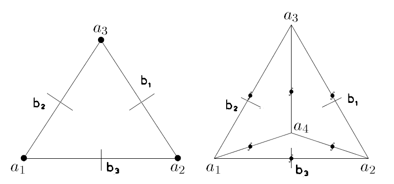
Fig. 3.1: The degrees of freedom of 2D Morley (left) and 3D Morley (right) element.

Let $V_{h}$ be the Morley finite element space

$$V_{h}=\{v_{h}:v_{h}|_{K}\in P_{2}(K),\forall K\in{\cal M}_{h},f(v_{h}|_{K_{1}})=f(v_{h}|_{K_{2}}),\forall f\in\Sigma_{K_{1}}\cap\Sigma_{K_{2}}\}.$$

The functions in $V_{h}$ may not be continuous in $\Omega$. Given a set $G\subset{\mathbf{R}}^{2}$, let ${\cal M}_{h}(G)=\{K\in{\cal M}_{h}:G\cap K\not=\emptyset\}$ and $N(G)$ the number of elements in ${\cal M}_{h}(G)$. For any $v_{h}\in V_{h}$, we define

$$\hat{v}_{h}(x_{i})=\frac{1}{N(x_{i})}\sum_{K^{\prime}\in{\cal M}_{h}(x_{i})}(v_{h}|_{K^{\prime}})(x_{i}),\ \ i=1,2,\cdots,n.$$ (3.2)

Notice that if $x_{i}$ is located inside some element $K$, then ${\cal M}_{h}(x_{i})=\{K\}$ and $\hat{v}_{h}(x_{i})=v_{h}(x_{i})$, $i=1,2,\cdots,n$. With this definition we know that $(\hat{v}_{h},\hat{w}_{h})_{n}$ and $(e,\hat{w}_{h})_{n}$ are well-defined for any $v_{h},w_{h}\in V_{h}$.

Let

$$a_{h}(u_{h},v_{h})=\sum_{K\in{\cal M}_{h}}\sum_{1\leq i,j\leq d}\int_{K}\frac{\partial^{2}u_{h}}{\partial x_{i}\partial x_{j}}\frac{\partial^{2}v_{h}}{\partial x_{i}\partial x_{j}}dx,\ \ \ \ \forall u_{h},v_{h}\in V_{h}.$$

The finite element approximation of the problem (3.1) is to find $u_{h}\in V_{h}$ such that

$$\lambda_{n}a_{h}(u_{h},v_{h})+(\hat{u}_{h},\hat{v}_{h})_{n}=(y,\hat{v}_{h})_{n},\ \ \ \ \forall v_{h}\in V_{h}.$$ (3.3)

Since the sampling point set $\mathbb{T}$ is not collinear, by Lax-Milgram lemma, the problem (3.3) has a unique solution.

Let $I_{K}:H^{2}(K)\to P_{2}(K)$ be the canonical local nodal value interpolant of Morley element [7, 9] and $I_{h}:L^{2}(\Omega)\to V_{h}$ be the global nodal value interpolant such that $(I_{h}u)|_{K}=I_{K}u$ for any $K\in{\cal M}_{h}$ and piecewise $H^{2}(K)$ functions $u\in L^{2}(\Omega)$. We introduce the mesh dependent semi-norm $|\cdot|_{m,h}$, $m\geq 0$,

$$|v|_{m,h}=\left(\sum_{K\in{\cal M}_{h}}|v|_{H^{m}(K)}^{2}\right)^{1/2},$$

for any $v\in L^{2}(\Omega)$ such that $v|_{K}\in H^{m}(K),\forall K\in{\cal M}_{h}$.

Lemma 3.3.

We have

$$|u-I_{K}u|_{H^{m}(K)}\leq Ch_{K}^{2-m}|u|_{H^{2}(K)},\ \ \forall u\in H^{m}(K),0\leq m\leq 2,$$ (3.4)

$$\|u-\widehat{I_{h}u}\|_{n}\leq Ch^{2}|u|_{H^{2}(\Omega)},\ \ \forall u\in H^{2}(\Omega),$$ (3.5)

where $h_{K}$ is the diameter of the element $K$ and $h=\max_{K\in{\cal M}_{h}}h_{K}$.

Proof.

Since $I_{K}p=p$ for any $p\in P_{2}(K)$ [9], the estimate (3.4) follows from the standard interpolation theory for finite element method [3]. Moreover, we have, by local inverse estimates and the standard interpolation estimates

$$\|u-I_{K}u\|_{L^{\infty}(K)} \leq \inf_{p\in P_{2}(K)}\left[\|u-p\|_{L^{\infty}(K)}+|K|^{-1/2}\|I_{K}(u-p)\|_{L^{2}(K)}\right]$$

$$\leq Ch_{K}^{2-d/2}|u|_{H^{2}(K)}.$$

Let $\mathbb{T}_{K}=\{x_{i}\in\mathbb{T}:x_{i}\in K,1\leq i\leq n\}$. By the assumption $\mathbb{T}$ is uniformly distributed and the mesh is quasi-uniform, we know that the cardinal $\#\mathbb{T}_{K}\leq Cnh^{d}$. Thus

$$\|u-\widehat{I_{h}u}\|_{n}^{2}\leq\frac{1}{n}\sum_{K\in{\cal M}_{h}}\#\mathbb{T}_{K}\|u-I_{K}u\|_{L^{\infty}(K)}^{2}\leq Ch^{4}|u|_{H^{2}(\Omega)}^{2}.$$

This proves (3.5). ∎

The following property of Morley element will be used below.

Lemma 3.4.

Let $K,K^{\prime}\in{\cal M}_{h}$ and $F=K\cap K^{\prime}$. There exists a constant C independent of $h$ such that for any $v_{h}\in V_{h}$, $|\alpha|\leq 2$,

$$\|\partial^{\alpha}(v_{h}|_{K}-v_{h}|_{K^{\prime}})\|_{L^{\infty}(F)}\leq Ch^{2-|\alpha|-d/2}(|v_{h}|_{H^{2}(K)}+|v_{h}|_{H^{2}(K^{\prime})}).$$

Proof.

By [9, Lemma 5] we know that

$$\|v_{h}|_{K}-v_{h}|_{K^{\prime}}\|_{L^{2}(F)}\leq Ch^{3/2}(|v_{h}|_{H^{2}(K)}+|v_{h}|_{H^{2}(K^{\prime})}).$$

By using the inverse estimate we then obtain

$$\|\partial^{\alpha}(v_{h}|_{K}-v_{h}|_{K^{\prime}})\|_{L^{\infty}(F)} \leq Ch^{-|\alpha|}\|v_{h}|_{K}-v_{h}|_{K^{\prime}}\|_{L^{\infty}(F)}$$

$$\leq Ch^{-|\alpha|-(d-1)/2}\|v_{h}|_{K}-v_{h}|_{K^{\prime}}\|_{L^{2}(F)}$$

$$\leq Ch^{2-|\alpha|-d/2}(|v_{h}|_{H^{2}(K)}+|v_{h}|_{H^{2}(K^{\prime})}).$$

This proves the lemma. ∎

Lemma 3.5.

There exists a linear operator $\Pi_{h}:V_{h}\to H^{2}(\Omega)$ such that for any $v_{h}\in V_{h}$,

$$|v_{h}-\Pi_{h}v_{h}|_{m,h}\leq Ch^{2-m}|v_{h}|_{2,h},\ \ m=0,1,2,$$ (3.6)

$$\|\hat{v}_{h}-\Pi_{h}v_{h}\|_{n}\leq Ch^{2}|v_{h}|_{2,h},$$ (3.7)

where the constant $C$ is independent of $h$.

Proof.

We will only prove the lemma for the case $d=2$. The case of $d=3$ will be briefly discussed in the appendix of this paper. We will construct $\Pi_{h}v_{h}$ by using the Agyris element. We recall [3, P.71] that for any $K\in{\cal M}_{h}$, Agyris element is a triple $(K,P_{K},\Lambda_{K})$, where $P_{K}=P_{5}(K)$ and the set of degrees of freedom, with the notation in Figure 3.2, $\Lambda_{K}=\{p(a_{i}),Dp(a_{i})(a_{j}-a_{i}),D^{2}p(a_{i})(a_{j}-a_{i},a_{k}-a_{i}),\partial_{\nu}p(b_{i}),1\leq i,j,k\leq 3,j\not=i,k\not=i,\forall p\in C^{2}(K)\}$. Let $X_{h}$ be the Agyris finite element space

$$X_{h}=\{v_{h}:v_{h}|_{K}\in P_{5}(K),\forall K\in{\cal M}_{h},f(v_{h}|_{K_{1}})=f(v_{h}|_{K_{2}}),\forall f\in\Lambda_{K_{1}}\cap\Lambda_{K_{2}}.\}$$

It is known that $X_{h}\subset H^{2}(\Omega)$.

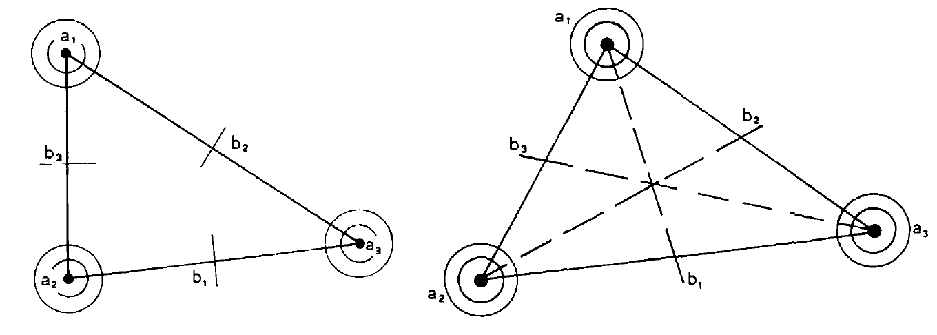
Fig. 3.2: The degrees of freedom of Agyris element (left) and Hermite triangle of type (5) (right).

We define the operator $\Pi_{h}$ as follows. For any $v_{h}\in V_{h}$, $w_{h}:=\Pi_{h}v_{h}\in X_{h}$ such that for any $K\in{\cal M}_{h}$, $w_{h}|_{K}\in P_{5}(K)$ and

$$\partial^{\alpha}(w_{h}|_{K})(a_{i})=\frac{1}{N(a_{i})}\sum_{K^{\prime}\in{\cal M}_{h}(a_{i})}\partial^{\alpha}(v_{h}|_{K^{\prime}})(a_{i}),\ \ 1\leq i\leq 3,\ \ |\alpha|\leq 2,$$ (3.8)

$$\partial_{\nu}(w_{h}|_{K})(b_{i})=\partial_{\nu}(v_{h}|_{K})(b_{i}),\ \ 1\leq i\leq 3.$$ (3.9)

Here ${\cal M}_{h}(a_{i})$ and $N(a_{i})$ are defined above (3.2). To show the estimate (3.6) we follow an idea in [3, Theorem 6.1.1] and use the element Hermite triangle of type (5) [3, P.102], which is a triple $(K,P_{K},\Theta_{K})$, where $P_{K}=P_{5}(K)$ and the set of degrees of freedom $\Theta_{K}=\{p(a_{i}),Dp(a_{i})(a_{j}-a_{i}),D^{2}p(a_{i})(a_{j}-a_{i},a_{k}-a_{i}),Dp(b_{i})(a_{i}-b_{i}),1\leq i,j,k\leq 3,j\not=i,k\not=i,\forall p\in C^{2}(K)\}$. The finite element space of Hermite triangle of type (5) is $H^{1}$ conforming and a regular family of Hermite triangle of type (5) is affine-equivalent. For any $K\in{\cal M}_{h}$, denote by $p_{i},p_{ij},p_{ijk},q_{i}$ the basis functions associated with the degrees of freedom $p(a_{i}),Dp(a_{i})(a_{j}-a_{i}),D^{2}p(a_{i})(a_{j}-a_{i},a_{k}-a_{i}),Dp(b_{i})(a_{i}-b_{i})$, $1\leq i,j,k\leq 3,j\not=i,k\not=i$.

For any $v_{h}\in V_{h}$, we also define a linear operator $q_{h}:=\Lambda_{h}v_{h}$ as follows: for any $K\in{\cal M}_{h}$, $q_{h}|_{K}\in P_{5}(K)$ and

$$\partial^{\alpha}(q_{h}|_{K})(a_{i})=\frac{1}{N(a_{i})}\sum_{K^{\prime}\in{\cal M}_{h}(a_{i})}\partial^{\alpha}(v_{h}|_{K^{\prime}})(a_{i}),\ \ 1\leq i\leq 3,\ \ |\alpha|\leq 2,$$ (3.10)

$$D(q_{h}|_{K})(b_{i})(a_{i}-b_{i})=D(v_{h}|_{K})(b_{i})(a_{i}-b_{i}),\ \ 1\leq i\leq 3.$$ (3.11)

Then from the definition of Morley element and Hermite triangle of type (5), we know that $\phi_{h}|_{K}:=(v_{h}-q_{h})|_{K}\in P_{5}(K)$ satisfies

$$\phi_{h}(x) = \sum_{i,j=1,2,3,j\not=i}D(\phi_{h}|_{K})(a_{i})(a_{j}-a_{i})p_{ij}(x)$$

$$+ \sum_{i,j,k=1,2,3,j\not=i,k\not=i}D^{2}(\phi_{h}|_{K})(a_{i})(a_{j}-a_{i},a_{k}-a_{i})p_{ijk}(x).$$

Since a regular family of Hermite triangle of type (5) is affine-equivalent, by standard scaling argument [3, Theorem 3.1.2], we obtain easily $|q_{i}|_{H^{m}(K)}+|p_{i}|_{H^{m}(K)}+|p_{ij}|_{H^{m}(K)}+|p_{ijk}|_{H^{m}(K)}\leq Ch_{K}^{1-m}$, $m=0,1,2$. Thus, for $m=0,1,2$,

$$|\phi_{h}|_{H^{m}(K)}\leq Ch_{K}^{1-m}\left(\sum_{i=1}^{3}\sum_{1\leq|\alpha|\leq 2}h^{|\alpha|}|\partial^{\alpha}(v_{h}|_{K})(a_{i})-\partial^{\alpha}(q_{h}|_{K})(a_{i})|^{2}\right)^{1/2}.$$ (3.12)

By Lemma 3.4 and the fact that $\partial^{\alpha}(q_{h}|_{K})(a_{i})$ is the local average of $\partial^{\alpha}v_{h}$ over elements around $a_{i}$ in (3.10)

$$|\partial^{\alpha}(v_{h}|_{K})(a_{i})-\partial^{\alpha}(q_{h}|_{K})(a_{i})|\leq Ch^{1-|\alpha|}\left(\sum_{K^{\prime}\in{\cal M}_{h}(a_{i})}|v_{h}|_{H^{2}(K^{\prime})}^{2}\right)^{1/2},\ \ \ \ \forall 1\leq|\alpha|\leq 2.$$

Inserting above estimate into (3.12), we get

$$|v_{h}-q_{h}|_{H^{m}(K)}\leq Ch^{2-m}\left(\sum_{K^{\prime}\in{\cal M}_{h}(K)}|v_{h}|_{H^{2}(K^{\prime})}^{2}\right)^{1/2},\ \ m=0,1,2.$$ (3.13)

By (3.8)-(3.11) we know that $q_{h}-w_{h}\in P_{5}(K)$ and satisfies

$$q_{h}(x)-w_{h}(x) = \sum\limits_{i=1}^{3}D(q_{h}|_{K}-w_{h}|_{K})(b_{i})(a_{i}-b_{i})q_{i}(x).$$

On the other hand, for $1\leq i\leq 3$,

$$D(q_{h}|_{K}-w_{h}|_{K})(b_{i})(a_{i}-b_{i})=\partial_{\nu}(q_{h}|_{K}-v_{h}|_{K})(b_{i})[(a_{i}-b_{i})\cdot\nu],$$

since $\partial_{\nu}(w_{h}|_{K})(b_{i})=\partial_{\nu}(v_{h}|_{K})(b_{i})$ by (3.9) and the tangential derivative of $(q_{h}|_{K}-w_{h}|_{K})$ vanishes as a consequence of (3.8) and (3.10). Since $|q_{i}|_{H^{m}(K)}\leq Ch_{K}^{1-m}$ for $m=0,1,2$, we obtain then

$$|q_{h}-w_{h}|_{H^{m}(K)} \leq Ch^{2-m}\left(\sum^{3}_{i=1}|\partial_{\nu}(q_{h}|_{K}-v_{h}|_{K})(b_{i})|^{2}\right)^{1/2}$$ (3.14)

$$\leq Ch^{2-m}\left(\sum_{K^{\prime}\in{\cal M}_{h}(K)}|v_{h}|_{H^{2}(K^{\prime})}^{2}\right)^{1/2},\ \ m=0,1,2,$$

where in the second inequality we have used the fact that by the inverse estimate and (3.13),

$$|\partial_{\nu}(q_{h}|_{K}-v_{h}|_{K})(b_{i})|\leq|q_{h}-v_{h}|_{W^{1,\infty}(K)} \leq Ch^{-1}_{K}|q_{h}-v_{h}|_{H^{1}(K)}$$

$$\leq C\left(\sum_{K^{\prime}\in{\cal M}_{h}(K)}|v_{h}|_{H^{2}(K^{\prime})}^{2}\right)^{1/2}.$$

Combining (3.13) and (3.14) shows (3.6).

To show (3.7), we use the notation in the proof of Lemma 3.3, the inverse estimate and (3.6) to get

$$\|\hat{v}_{h}-w_{h}\|_{n}^{2}\leq\frac{C}{n}\sum_{K\in{\cal M}_{h}}\#\mathbb{T}_{K}\|v_{h}-w_{h}\|_{L^{\infty}(K)}^{2}\leq C\|v_{h}-w_{h}\|^{2}_{L^{2}(\Omega)}\leq Ch^{4}|v_{h}|_{2,h}^{2}.$$

This completes the proof. ∎

For any function $v$ which is piecewise in $C^{2}(K)$ for any $K\in{\cal M}_{h}$, we use the convenient energy norm

$$|{\hskip-1.0pt}\|v|{\hskip-1.0pt}\|_{h}=\left(\lambda_{n}|v|_{2,h}^{2}+\|\hat{v}\|_{n}^{2}\right)^{1/2}.$$

Here $\hat{v}(x_{i})$, $i=1,2,\cdots,n$, is defined as in (3.2), that is, $\hat{v}(x_{i})$ is the local average of all $v|_{K^{\prime}}(x_{i})$, where $K^{\prime}\in{\cal M}_{h}$ such that $x_{i}\in K^{\prime}$.

Theorem 3.6.

Let $u_{n}\in H^{2}(\Omega)$ be the unique solution of (3.1) and $u_{h}\in V_{h}$ be the solution of (3.3). Then there exist constants $\lambda_{0}>0$ and $C>0$ such that for any $\lambda_{n}\leq\lambda_{0}$ and $n\lambda_{n}^{d/4}\geq 1$,

$$\mathbb{E}\big{[}\|u_{0}-\hat{u}_{h}\|_{n}^{2}\big{]}\leq C(\lambda_{n}+h^{4})|u_{0}|^{2}_{H^{2}(\Omega)}+C\left[1+\frac{h^{4}}{\lambda_{n}}+\left(\frac{h^{4}}{\lambda_{n}}\right)^{1-d/4}\right]\frac{\sigma^{2}}{n\lambda_{n}^{d/4}}.$$ (3.15)

In particular, if $h^{4}\leq C\lambda_{n}$, we have

$$\mathbb{E}\big{[}\|u_{0}-\hat{u}_{h}\|_{n}^{2}\big{]}\leq C\lambda_{n}|u_{0}|_{H^{2}(\Omega)}^{2}+\frac{C\sigma^{2}}{n\lambda_{n}^{d/4}}.$$ (3.16)

Proof.

We start by using the Strang lemma [3]

$$|{\hskip-1.0pt}\|u_{n}-\hat{u}_{h}|{\hskip-1.0pt}\|_{h}\leq C\inf_{v_{h}\in V_{h}}|{\hskip-1.0pt}\|u_{n}-\hat{v}_{h}|{\hskip-1.0pt}\|_{h}+C\sup_{0\not=v_{h}\in V_{h}}\frac{|\lambda_{n}a_{h}(u_{n},v_{h})+(u_{n}-y,\hat{v}_{h})_{n}|}{|{\hskip-1.0pt}\|v_{h}|{\hskip-1.0pt}\|_{h}}.$$ (3.17)

By Lemma 3.3 we have

$$\inf_{v_{h}\in V_{h}}|{\hskip-1.0pt}\|u_{n}-\hat{v}_{h}|{\hskip-1.0pt}\|_{h}\leq C(\lambda_{n}^{1/2}+h^{2})|u_{n}|_{H^{2}(\Omega)}.$$ (3.18)

Since for any $v_{h}\in V_{h}$, $\Pi_{h}v_{h}\in H^{2}(\Omega)$, by (3.1) and the fact that $y_{i}=u_{0}(x_{i})+e_{i}$, $i=1,2,\cdots n$, to obtain

$$\lambda_{n}a_{h}(u_{n},v_{h})+(u_{n}-y,\hat{v}_{h})_{n}$$

$$= \lambda_{n}a_{h}(u_{n},v_{h}-\Pi_{h}v_{h})+(u_{n}-y,\hat{v}_{h}-\Pi_{h}v_{h})_{n}$$

$$\leq \lambda_{n}|u_{n}|_{H^{2}(\Omega)}|v_{h}-\Pi_{h}v_{h}|_{2,h}+\|u_{n}-u_{0}\|_{n}\|\hat{v}_{h}-\Pi_{h}v_{h}\|_{n}+(e,\hat{v}_{h}-\Pi_{h}v_{h})_{n}.$$

Now by using Lemma 3.5 we have

$$\sup_{0\not=v_{h}\in V_{h}}\frac{|\lambda_{n}a_{h}(u_{n},v_{h})+(u_{n}-y,\hat{v}_{h})_{n}|}{|{\hskip-1.0pt}\|v_{h}|{\hskip-1.0pt}\|_{h}}$$ (3.19)

$$\leq C\lambda_{n}^{1/2}|u_{n}|_{H^{2}(\Omega)}+C\frac{h^{2}}{\lambda_{n}^{1/2}}\|u_{n}-u_{0}\|_{n}+\sup_{0\not=v_{h}\in V_{h}}\frac{|(e,\hat{v}_{h}-\Pi_{h}v_{h})_{n}|}{|{\hskip-1.0pt}\|v_{h}|{\hskip-1.0pt}\|_{h}}.$$

Since $e_{i}$, $i=1,2,\cdots,n$, are independent and identically distributed random variables, we have

$$\mathbb{E}\big{[}|(e,\hat{v}_{h}-\Pi_{h}v_{h})_{n}|^{2}\big{]}=\sigma^{2}n^{-1}\|\hat{v}_{h}-\Pi_{h}v_{h}\|_{n}^{2}\leq C\sigma^{2}n^{-1}h^{4}|v_{h}|_{2,h}^{2},$$

where we have used Lemma 3.5 in the last inequality.

Let $N_{h}$ be the dimension of $V_{h}$ which satisfies $N_{h}\leq Ch^{-d}$ since the mesh is quasi-uniform. Recall that if $\{X_{i}\}_{i=1}^{N_{h}}$ are random variables, ${\mathbb{E}}[\sup_{1\leq i\leq N_{h}}|X_{i}|]\leq\sum^{N_{h}}_{i=1}{\mathbb{E}}[|X_{i}|]$. We have then

$$\mathbb{E}\left[\sup_{0\not=v_{h}\in V_{h}}\frac{|(e,v_{h}-\Pi_{h}v_{h})_{n}|^{2}}{|{\hskip-1.0pt}\|v_{h}|{\hskip-1.0pt}\|_{h}^{2}}\right]\leq N_{h}\cdot\sup_{0\not=v_{h}\in V_{h}}\mathbb{E}\left[\frac{|(e,v_{h}-\Pi_{h}v_{h})_{n}|^{2}}{|{\hskip-1.0pt}\|v_{h}|{\hskip-1.0pt}\|_{h}^{2}}\right]\leq C\frac{\sigma^{2}h^{4-d}}{n\lambda_{n}}.$$ (3.20)

Combining (3.17)-(3.20) we obtain

$$\mathbb{E}\big{[}|{\hskip-1.0pt}\|u_{n}-\hat{u}_{h}|{\hskip-1.0pt}\|_{h}^{2}\big{]}\leq C\lambda_{n}\mathbb{E}\big{[}|u_{n}|_{H^{2}(\Omega)}^{2}\big{]}+C\frac{h^{4}}{\lambda_{n}}\mathbb{E}\big{[}\|u_{n}-u_{0}\|_{n}^{2}\big{]}+C\frac{\sigma^{2}h^{4-d}}{n\lambda_{n}}.$$

This completes the proof by using Theorem 2.2. ∎

4 Stochastic convergence

In this section we study the stochastic convergence of the error $\|u_{0}-\hat{u}_{h}\|_{n}$ which characterizes the tail property of $\mathbb{P}(\|u_{0}-\hat{u}_{h}\|_{n}\geq z)$ for $z>0$. We assume the noises $e_{i}$, $i=1,2,\cdots,n$, are independent and identically distributed sub-Gaussian random variables with parameter $\sigma>0$. A random variable $X$ is sub-Gaussion with parameter $\sigma$ if it satisfies

$$\mathbb{E}\left[e^{\lambda(X-\mathbb{E}[X])}\right]\leq e^{\frac{1}{2}\sigma^{2}\lambda^{2}},\ \ \ \ \forall\lambda\in{\mathbf{R}}.$$ (4.1)

The probability distribution function of a sub-Gaussion random variable has a exponentially decaying tail, that is, if $X$ is a sub-Gaussion random variable, then

$$\mathbb{P}(|X-{\mathbb{E}}[X]|\geq z)\leq 2e^{-\frac{1}{2}z^{2}/\sigma^{2}},\ \ \forall z>0.$$ (4.2)

In fact, by Markov inequality, for any $\lambda>0$,

$$\mathbb{P}(X-{\mathbb{E}}[X]\geq z)=\mathbb{P}(\lambda(X-{\mathbb{E}}[X])\geq\lambda z)\leq e^{-\lambda z}{\mathbb{E}}[e^{\lambda(X-{\mathbb{E}}[X])}]\leq e^{-\lambda z-\frac{1}{2}\sigma^{2}\lambda^{2}}.$$

By taking $\lambda=z/\sigma^{2}$ yields $\mathbb{P}(X-{\mathbb{E}}[X]\geq z)\leq e^{-\frac{1}{2}z^{2}/\sigma^{2}}$. Similarly, one can prove $\mathbb{P}(X-{\mathbb{E}}[X]\leq-z)\leq e^{-\frac{1}{2}z^{2}/\sigma^{2}}$. This shows (4.2).

4.1 Stochastic convergence of the thin plate splines

We will use several tools from the theory of empirical processes [11, 10] for our analysis. We start by recalling the definition of Orlicz norm. Let $\psi$ be a monotone increasing convex function satisfying $\psi(0)=0$. Then the Orilicz norm $\|X\|_{\psi}$ of a random variable $X$ is defined as

$$\|X\|_{\psi}=\inf\left\{C>0:\mathbb{E}\left[\psi\left(\frac{|X|}{C}\right)\right]\leq 1\right\}.$$ (4.3)

By using Jensen inequality, it is easy to check $\|X\|_{\psi}$ is a norm. In the following we will use the $\|X\|_{\psi_{2}}$ norm with $\psi_{2}(t)=e^{t^{2}}-1$ for any $t>0$. By definition we know that

$$\mathbb{P}(|X|\geq z)\leq 2\,e^{-z^{2}/\|X\|_{\psi_{2}}^{2}},\ \ \ \ \forall z>0.$$ (4.4)

The following lemma is from [11, Lemma 2.2.1] which shows the inverse of this property.

Lemma 4.7.

If there exist positive constants $C,K$ such that $\mathbb{P}(|X|>z)\leq Ke^{-Cz^{2}},\ \forall z>0$, then $\|X\|_{\psi_{2}}\leq\sqrt{(1+K)/C}$.

Let $T$ be a semi-metric space with the semi-metric $d$ and $\{X_{t}:t\in T\}$ be a random process indexed by $T$. Then the random process $\{X_{t}:t\in T\}$ is called sub-Gaussian if

$$\mathbb{P}(|X_{s}-X_{t}|>z)\leq 2e^{-\frac{1}{2}z^{2}/d(s,t)^{2}},\ \ \ \ \forall s,t\in T,\ \ z>0.$$ (4.5)

For a semi-metric space $(T,d)$, an important quantity to characterize the complexity of the set $T$ is the entropy which we now introduce. The covering number $N(\varepsilon,T,d)$ is the minimum number of $\varepsilon$-balls that cover $T$. A set is called $\varepsilon$-separated if the distance of any two points in the set is strictly greater than $\varepsilon$. The packing number $D(\varepsilon,T,d)$ is the maximum number of $\varepsilon$-separated points in $T$. $\log N(\varepsilon,T,d)$ is called the covering entropy and $\log D(\varepsilon,T,d)$ is called the packing entropy. It is easy to check that [11, P.98]

$$N(\varepsilon,T,d)\leq D(\varepsilon,T,d)\leq N(\frac{\varepsilon}{2},T,d).$$ (4.6)

The following maximal inequality [11, Section 2.2.1] plays an important role in our analysis.

Lemma 4.8.

If $\{X_{t}:t\in T\}$ is a separable sub-Gaussian random process, then

$$\|\sup_{s,t\in T}|X_{s}-X_{t}|\|_{\psi_{2}}\leq K\int^{\mathrm{diam}\,T}_{0}\sqrt{\log D(\varepsilon,T,d)}\ d\varepsilon.$$

Here $K>0$ is some constant.

The following result on the estimation of the entropy of Sobolev spaces is due to Birman-Solomyak [2].

Lemma 4.9.

Let $Q$ be the unit square in ${\mathbf{R}}^{d}$ and $SW^{\alpha,p}(Q)$ be the unit sphere of the Sobolev space $W^{\alpha,p}(Q)$, where $\alpha>0,p\geq 1$. Then for $\varepsilon>0$ sufficient small, the entropy

$$\log N(\varepsilon,SW^{\alpha,p}(Q),\|\cdot\|_{L^{q}(Q)})\leq C\varepsilon^{-d/\alpha},$$

where if $\alpha p>d$, $1\leq q\leq\infty$, otherwise if $\alpha p\leq d$, $1\leq q\leq q^{*}$ with $q^{*}=p(1-\alpha p/d)^{-1}$.

For any $\delta>0,\rho>0$, define

$$S_{\delta,\rho}(\Omega):=\{u\in H^{2}(\Omega):\|u\|_{n}\leq\delta,|u|_{H^{2}(\Omega)}\leq\rho\}.$$ (4.7)

The following lemma estimates the entropy of the set $S_{\delta,\rho}(\Omega)$.

Lemma 4.10.

There exists a constant $C$ independent of $\delta,\rho,\varepsilon$ such that

$$\log N(\varepsilon,S_{\delta,\rho}(\Omega),\|\cdot\|_{L^{\infty}(\Omega)})\leq C\left(\frac{\rho+\delta}{\varepsilon}\right)^{d/2}.$$

Proof.

By (2.1) we have for any $u\in S_{\delta,\rho}(\Omega)$, $\|u\|_{H^{2}(\Omega)}\leq C(\|u\|_{L^{2}(\Omega)}+|u|_{H^{2}(\Omega)})\leq C(\|u\|_{n}+|u|_{H^{2}(\Omega)})\leq C(\delta+\rho)$, where we have used the fact that $h_{\max}\leq Cn^{-1/d}\leq C$. The lemma now follows from Lemma 4.9. ∎

The following lemma is proved by the argument in [11, Lemma 2.2.7].

Lemma 4.11.

$\{E_{n}(u):=(e,u)_{n}:u\in H^{2}(\Omega)\}$ is a sub-Gaussian random process with respect to the semi-distance $d(u,v)=\|u-v\|_{n}^{*}$, where $\|u\|^{*}_{n}:=\sigma n^{-1/2}\|u\|_{n}$.

Proof.

By definition $E_{n}(u)-E_{n}(v)=\sum^{n}_{i=1}c_{i}e_{i}$, where $c_{i}=\frac{1}{n}(u-v)(x_{i})$. Since $e_{i}$ is a sub-Gaussion random variable with parameter $\sigma$ and ${\mathbb{E}}[e_{i}]=0$, by (4.1), ${\mathbb{E}}[e^{\lambda e_{i}}]\leq e^{\frac{1}{2}\sigma^{2}\lambda^{2}},\forall\lambda>0$. Thus, since $e_{i}$, $i=1,2,\cdots,n$, are independent random variables,

$${\mathbb{E}}\left[e^{\lambda\sum^{n}_{i=1}c_{i}e_{i}}\right]\leq e^{\frac{1}{2}\sigma^{2}\lambda^{2}\sum^{n}_{i=1}c_{i}^{2}}=e^{\frac{1}{2}\sigma^{2}n^{-1}\lambda^{2}\|u-v\|_{n}^{2}}=e^{\frac{1}{2}d(u,v)^{2}\lambda^{2}}.$$

This shows $E_{n}(u)-E_{n}(v)$ is a sub-Gaussion random variable with parameter $d(u,v)$. By (4.2) we have

$$\mathbb{P}(|E_{n}(u)-E_{n}(v)|\geq z)\leq 2e^{-\frac{1}{2}z^{2}/d(u,v)^{2}},\ \ \forall z>0.$$

This shows the lemma by the definition of sub-Gaussion random process (4.5). ∎

The following lemma which improves Lemma 4.7 will be used in our subsequent analysis.

Lemma 4.12.

If $X$ is a random variable which satisfies

$$\mathbb{P}(|X|>\alpha(1+z))\leq C_{1}e^{-z^{2}/K_{1}^{2}},\ \ \forall\alpha>0,z\geq 1,$$

where $C_{1},K_{1}$ are some positive constants, then $\|X\|_{\psi_{2}}\leq C(C_{1},K_{1})\alpha$ for some constant $C(C_{1},K_{1})$ depending only on $C_{1},K_{1}$.

Proof.

If $y\geq 2\alpha$, then $z=(y/\alpha)-1\geq 1$. Thus

$$\mathbb{P}(|X|>y)=\mathbb{P}(|X|>\alpha(1+z))\leq C_{1}\exp\left[-\frac{1}{K_{1}^{2}}\left(\frac{y}{\alpha}-1\right)^{2}\right].$$

Since $(\frac{y}{\alpha}-1)^{2}\geq\frac{1}{2}(\frac{y}{\alpha})^{2}-1$ by Cauchy-Schwarz inequality, we obtain

$$\mathbb{P}(|X|>y)\leq C_{1}e^{\frac{1}{K_{1}^{2}}}e^{-\frac{y^{2}}{2K_{1}^{2}\alpha^{2}}}=C_{1}e^{\frac{1}{K_{1}^{2}}}e^{-\frac{y^{2}}{K^{2}_{2}}},$$

where $K_{2}:=\sqrt{2}\alpha K_{1}$. On the other hand, if $y<2\alpha$, then

$$\mathbb{P}(|X|>y)\leq e^{\frac{y^{2}}{K_{2}^{2}}}e^{-\frac{y^{2}}{K_{2}^{2}}}\leq e^{\frac{2}{K^{2}_{1}}}e^{-\frac{y^{2}}{K_{2}^{2}}}.$$

Therefore, $\mathbb{P}(|X|>y)\leq C_{2}e^{-y^{2}/K_{2}^{2}}$, $\forall y>0$, where $C_{2}=\max(C_{1}e^{1/{K_{1}^{2}}},e^{2/K_{1}^{2}})$. This implies by Lemma 4.7,

$$\|X\|_{\psi_{2}}\leq\sqrt{1+C_{2}}K_{2}=C(C_{1},K_{1})\alpha,\ \ \mbox{where }C(C_{1},K_{1})=\sqrt{2}K_{1}\sqrt{1+C_{2}}.$$

This completes the proof. ∎

Theorem 4.13.

Let $u_{n}\in H^{2}(\Omega)$ be the solution of (3.1). Denote by $\rho_{0}=|u_{0}|_{H^{2}(\Omega)}+\sigma n^{-1/2}$. If we take

$$\lambda_{n}^{1/2+d/8}=O(\sigma n^{-1/2}\rho_{0}^{-1}),$$ (4.8)

then there exists a constant $C>0$ such that

$$\|\,\|u_{n}-u_{0}\|_{n}\,\|_{\psi_{2}}\leq C\lambda_{n}^{1/2}\rho_{0},\ \ \ \ \|\,|u_{n}|_{H^{2}(\Omega)}\,\|_{\psi_{2}}\leq C\rho_{0}.$$ (4.9)

Proof.

We will only prove the first estimate in (4.9) by the peeling argument. The other estimate can be proved in a similar way. It follows from (2.8) that

$$\|u_{n}-u_{0}\|^{2}_{n}+\lambda_{n}|u_{n}|_{H^{2}(\Omega)}^{2}\leq 2(e,u_{n}-u_{0})_{n}+\lambda_{n}|u_{0}|_{H^{2}(\Omega)}^{2}.$$ (4.10)

Let $\delta>0,\ \rho>0$ be two constants to be determined later, and

$$A_{0}=[0,\delta),A_{i}=[2^{i-1}\delta,2^{i}\delta),\ \ B_{0}=[0,\rho),B_{j}=[2^{j-1}\rho,2^{j}\rho),\ \ \ \ i,j\geq 1.$$ (4.11)

For $i,j\geq 0$, define

$$F_{ij}=\{v\in H^{2}(\Omega):~{}\|v\|_{n}\in A_{i}~{},~{}|v|_{H^{2}(\Omega)}\in B_{j}\}.$$

Then we have

$$\mathbb{P}(\|u_{n}-u_{0}\|_{n}>\delta)\leq\sum_{i=1}^{\infty}\sum_{j=0}^{\infty}\mathbb{P}(u_{n}-u_{0}\in F_{ij}).$$ (4.12)

Now we estimate $\mathbb{P}(u_{n}-u_{0}\in F_{ij})$. By Lemma 4.11, $\{(e,v)_{n}:v\in H^{2}(\Omega)\}$ is a sub-Gaussion random process with respect to the semi-distance $d(u,v)=\sigma n^{-1/2}\|u-v\|_{n}$. It is easy to see that

$$\mathrm{diam}\,F_{ij}\leq\sigma n^{-1/2}\sup_{u-u_{0},v-u_{0}\in F_{ij}}(\|u-u_{0}\|_{n}+\|v-u_{0}\|_{n})\leq 2\sigma n^{-1/2}\cdot 2^{i}\delta.$$

Then by (4.6) and the maximal inequality in Lemma 4.8 we have

$$\|\sup_{u-u_{0}\in F_{ij}}|(e,u-u_{0})_{n}|\|_{\psi_{2}} \leq K\int^{\sigma n^{-1/2}\cdot 2^{i+1}\delta}_{0}\sqrt{\log N\left(\frac{\varepsilon}{2},F_{ij},d\right)}\,d\varepsilon$$

$$= K\int^{\sigma n^{-1/2}\cdot 2^{i+1}\delta}_{0}\sqrt{\log N\left(\frac{\varepsilon}{2\sigma n^{-1/2}},F_{ij},\|\cdot\|_{n}\right)}\,d\varepsilon.$$

By Lemma 4.10 we have the estimate for the entropy

$$\log N\left(\frac{\varepsilon}{2\sigma n^{-1/2}},F_{ij},\|\cdot\|_{n}\right) \leq \log N(\frac{\varepsilon}{2\sigma n^{-1/2}},F_{ij},\|\cdot\|_{L^{\infty}(\Omega)})$$

$$\leq C\left(\frac{2\sigma n^{-1/2}\cdot(2^{i}\delta+2^{j}\rho)}{\varepsilon}\right)^{d/2}.$$

Therefore,

$$\|\sup_{u-u_{0}\in F_{ij}}|(e,u-u_{0})_{n}\|_{\psi_{2}} \leq K\int^{\sigma n^{-1/2}\cdot 2^{i+1}\delta}_{0}\left(\frac{2\sigma n^{-1/2}\cdot(2^{i}\delta+2^{j}\rho)}{\varepsilon}\right)^{d/4}\,d\varepsilon$$ (4.13)

$$= C\sigma n^{-1/2}(2^{i}\delta+2^{j}\rho)^{d/4}(2^{i}\delta)^{1-d/4}$$

$$\leq C\sigma n^{-1/2}[2^{i}\delta+(2^{i}\delta)^{1-d/4}(2^{j}\rho)^{d/4}].$$

By (4.10) and (4.4) we have for $i,j\geq 1$:

$$\mathbb{P}(u_{n}-u_{0}\in F_{ij}) \leq \mathbb{P}(2^{2(i-1)}\delta^{2}+\lambda_{n}2^{2(j-1)}\rho^{2}\leq 2\mathop{\sup}\limits_{u-u_{0}\in F_{ij}}|(e,u-u_{0})_{n}|+\lambda_{n}\rho^{2}_{0})$$

$$= \mathbb{P}(2\mathop{\sup}\limits_{u-u_{0}\in F_{ij}}|(e,u-u_{0})_{n}|\geq 2^{2(i-1)}\delta^{2}+\lambda_{n}2^{2(j-1)}\rho^{2}-\lambda_{n}\rho^{2}_{0})$$

$$\leq 2\exp\left[-\frac{1}{C\sigma^{2}n^{-1}}\left(\frac{2^{2(i-1)}\delta^{2}+\lambda_{n}2^{2(j-1)}\rho^{2}-\lambda_{n}\rho^{2}_{0}}{2^{i}\delta+(2^{i}\delta)^{1-d/4}(2^{j}\rho)^{d/4}}\right)^{2}\right].$$

Now we take

$$\delta^{2}=\lambda_{n}\rho_{0}^{2}(1+z)^{2},\ \rho=\rho_{0},\ \ \mbox{where }z\geq 1.$$ (4.14)

Since by assumption $\lambda_{n}^{1/2+d/8}=O(\sigma n^{-1/2}\rho_{0}^{-1})$ and $\sigma n^{-1/2}\rho_{0}^{-1}\leq 1$, we have $\lambda_{n}\leq C$ for some constant. By some simple calculation we have for $i,j\geq 1$,

$$\mathbb{P}(u_{n}-u_{0}\in F_{ij}) \leq 2\exp\left[-C\left(\frac{2^{2(i-1)}z(1+z)+2^{2(j-1)}}{2^{i}(1+z)+(2^{i}(1+z))^{1-d/4}(2^{j})^{d/4}}\right)^{2}\right].$$

By using the elementary inequality $ab\leq\frac{1}{p}a^{p}+\frac{1}{q}b^{q}$ for any $a,b>0,p,q>1,p^{-1}+q^{-1}=1$, we have $(2^{i}(1+z))^{1-d/4}(2^{j})^{d/4}\leq(1+z)2^{i}+2^{j}$. Thus

$$\mathbb{P}(u_{n}-u_{0}\in F_{ij})\leq 2\exp\left[-C(2^{2i}z^{2}+2^{2j})\right].$$

Similarly, one can prove for $i\geq 1,j=0$,

$$\mathbb{P}(u_{n}-u_{0}\in F_{i0})\leq 2\exp\left[-C(2^{2i}z^{2})\right].$$

Therefore, since $\sum^{\infty}_{j=1}e^{-C(2^{2j})}\leq e^{-C}<1$ and $\sum^{\infty}_{i=1}e^{-C(2^{2i}z^{2})}\leq e^{-Cz^{2}}$, we obtain finally

$$\sum_{i=1}^{\infty}\sum_{j=0}^{\infty}\mathbb{P}(u_{n}-u_{0}\in F_{ij}) \leq 2\sum_{i=1}^{\infty}\sum_{j=1}^{\infty}e^{-C(2^{2i}z^{2}+2^{2j})}+2\sum^{\infty}_{i=1}e^{-C(2^{2i}z^{2})}$$

$$\leq 4e^{-Cz^{2}}.$$

Now inserting the estimate to (4.12) we have

$$\mathbb{P}(\|u_{n}-u_{0}\|_{n}>\lambda_{n}^{1/2}\rho_{0}(1+z))\leq 4e^{-Cz^{2}},\ \ \ \ \forall z\geq 1.$$ (4.15)

This implies by using Lemma 4.12 that $\|\|u_{n}-u_{0}\|_{n}\|_{\psi_{2}}\leq C\lambda_{n}^{1/2}\rho_{0}$. This completes the proof. ∎

We remark that (4.15) implies that

$$\lim_{z\to\infty}\overline{\lim_{n\to\infty}}\ \mathbb{P}(\|u_{n}-u_{0}\|_{n}>\lambda_{n}^{1/2}\rho_{0}(1+z))=0.$$

In terms of the terminology of the stochastic convergence order, we have $\|u_{n}-u_{0}\|_{n}=O_{p}(\lambda_{n}^{1/2})\rho_{0}$ which by the assumption (4.8) yields

$$\|u_{n}-u_{0}\|_{n}=O_{p}(n^{-\frac{2}{4+d}})\sigma^{\frac{4}{4+d}}\rho_{0}^{-\frac{4}{4+d}}.$$

This estimate is proved in [10, Section 10.1.1] when $d=1$. Our result in Theorem 4.13 is stronger in the sense that it also provides the tail property of the probability distribution function of the random error $\|u_{n}-u_{0}\|_{n}$.

4.2 Stochastic convergence of the finite element method

The following lemma provides the estimate of the entropy of finite dimension subsets [10, Corollary 2.6].

Lemma 4.14.

Let $G$ be a finite dimensional subspace of $L^{2}(\Omega)$ of dimension $N>0$ and $G_{R}=\{f\in G:\|f\|_{L^{2}(\Omega)}\leq R\}$. Then

$$N(\varepsilon,G_{R},\|\cdot\|_{L^{2}(\Omega)})\leq(1+4R/\varepsilon)^{N},\ \ \forall\varepsilon>0.$$

Lemma 4.15.

Let $G_{h}:=\{v_{h}\in V_{h}:|{\hskip-1.0pt}\|v_{h}|{\hskip-1.0pt}\|_{h}=(\lambda_{n}|v_{h}|_{2,h}^{2}+\|\hat{v}_{h}\|_{n}^{2})^{1/2}\leq 1\}$. Assume that $h=O(\lambda_{n}^{1/4})$ and $n\lambda_{n}^{d/4}\geq 1$. Then

$$\|\,\sup_{v_{h}\in G_{h}}|(e,\hat{v}_{h}-\Pi_{h}v_{h})_{n}|\,\|_{\psi_{2}}\leq C\sigma n^{-1/2}\lambda_{n}^{-d/8}.$$

Proof.

Similar to the proof of Lemma 4.11 we know that $\{\hat{E}_{n}(v_{h}):=(e,\hat{v}_{h}-\Pi_{h}v_{h})_{n},\ \forall v_{h}\in G_{h}\}$ is a sub-Gaussion random process with respect to the semi-distance $\hat{d}(v_{h},w_{h})=\sigma n^{-1/2}\|(\hat{v}_{h}-\Pi_{h}v_{h})-(\hat{w}_{h}-\Pi_{h}w_{h})\|_{n}$. By Lemma 3.5, for any $v_{h}\in G_{h}$, $\|\hat{v}_{h}-\Pi_{h}v_{h}\|_{n}\leq Ch^{2}|v_{h}|_{2,h}\leq Ch^{2}\lambda_{n}^{-1/2}\leq C$, where we have used the assumption $h=O(\lambda_{n}^{1/4})$ in the last inequality. This implies that the diameter of $G_{h}$ is bounded by $C\sigma n^{-1/2}$. Now by the maximal inequality in Lemma 4.8

$$\|\,\sup_{v_{h}\in G_{h}}|(e,\hat{v}_{h}-\Pi_{h}v_{h})_{n}|\,\|_{\psi_{2}}\leq K\int_{0}^{C\sigma n^{-1/2}}\sqrt{\log N\left(\frac{\varepsilon}{2},G_{h},\hat{d}\right)}\ d\varepsilon.$$ (4.16)

For any $v_{h}\in V_{h}$, by Lemma 3.5, $\Pi_{h}v_{h}\in H^{2}(\Omega)$ and thus by (2.1)

$$\|\Pi_{h}v_{h}\|_{L^{2}(\Omega)} \leq C(h^{2}_{\max}|\Pi_{h}v_{h}|_{H^{2}(\Omega)}+\|\Pi_{h}v_{h}\|_{n})$$

$$\leq C(n^{-2/d}\lambda_{n}^{-1/2}+\|\Pi_{h}v_{h}-\hat{v}_{h}\|_{n}+\|\hat{v}_{h}\|_{n})$$

$$\leq C(n^{-2/d}\lambda_{n}^{-1/2}+Ch^{2}\lambda_{n}^{-1/2}+1)$$

$$\leq C,$$

where we have used $h=O(\lambda_{n}^{1/4})$ and $n\lambda_{n}^{d/4}\geq 1$ in the last inequality. Thus

$$\|v_{h}\|_{L^{2}(\Omega)}\leq\|v_{h}-\Pi_{h}v_{h}\|_{L^{2}(\Omega)}+\|\Pi_{h}v_{h}\|_{L^{2}(\Omega)}\leq Ch^{2}|v_{h}|_{2,h}+C\leq C,\ \ \ \ \forall v_{h}\in G_{h}.$$ (4.17)

Moreover, by Lemma 3.5 and inverse estimate,

$$\hat{d}(v_{h},w_{h})\leq C\sigma n^{-1/2}h^{2}|v_{h}-w_{h}|_{2,h}\leq C\sigma n^{-1/2}\|v_{h}-w_{h}\|_{L^{2}(\Omega)},\ \ \ \ \forall v_{h},w_{h}\in V_{h}.$$ (4.18)

Now since the dimension of $V_{h}$ is bounded by $Ch^{-d}$, Lemma 4.14 together with (4.17)-(4.18) implies

$$\log N\left(\frac{\varepsilon}{2},G_{h},\hat{d}\right) = \log N\left(\frac{\varepsilon}{C\sigma n^{-1/2}},G_{h},\|\cdot\|_{L^{2}(\Omega)}\right)$$

$$\leq Ch^{-d}(1+{\sigma n^{-1/2}}/\varepsilon).$$

Inserting this estimate to (4.16)

$$\|\,\sup_{v_{h}\in G_{h}}|(e,\hat{v}_{h}-\Pi_{h}v_{h})_{n}|\,\|_{\psi_{2}} \leq C\int_{0}^{C\sigma n^{-1/2}}\sqrt{Ch^{-d}(1+\sigma n^{-1/2}/\varepsilon)}\,d\varepsilon$$

$$\leq Ch^{-d/2}\sigma n^{-1/2}.$$

This completes the proof since $h=O(\lambda_{n}^{1/4})$. ∎

The following theorem is the main result of this section.

Theorem 4.16.

Let $u_{h}\in V_{h}$ be the solution of (3.3). Denote by $\rho_{0}=|u_{0}|_{H^{2}(\Omega)}+\sigma n^{-1/2}$. If we take

$$h=O(\lambda_{n}^{1/4})\ \ \mbox{and }\ \lambda_{n}^{1/2+d/8}=O(\sigma n^{-1/2}\rho_{0}^{-1}),$$ (4.19)

then there exists a constant $C>0$ such that

$$\|\,\|\hat{u}_{h}-u_{0}\|_{n}\,\|_{\psi_{2}}\leq C\lambda_{n}^{1/2}\rho_{0},\ \ \ \ \|\,|u_{h}|_{H^{2}(\Omega)}\,\|_{\psi_{2}}\leq C\rho_{0}.$$ (4.20)

Proof.

By (3.17)-(3.19) we have

$$\lambda_{n}^{1/2}|u_{h}|_{H^{2}(\Omega)}+\|\hat{u}_{h}-u_{0}\|_{n}$$

$$\leq C(1+\frac{h^{2}}{\lambda_{n}^{1/2}})\|u_{n}-u_{0}\|_{n}+C(h^{2}+\lambda_{n}^{1/2})(|u_{n}|_{H^{2}(\Omega)}+|u_{0}|_{H^{2}(\Omega)})$$

$$+ C\sup_{0\not=v_{h}\in V_{h}}\frac{|(e,\hat{v}_{h}-\Pi_{h}v_{h})_{n}|}{|{\hskip-1.0pt}\|v_{h}|{\hskip-1.0pt}\|_{h}}.$$

The theorem follows now from Theorem 4.13, Lemma 4.15 and the assumption $\sigma n^{-1/2}\leq C\lambda_{n}^{1/2+d/8}\rho_{0}$. ∎

By (4.4), we know from Theorem 4.16 that

$$\mathbb{P}(\|\hat{u}_{h}-u_{0}\|_{n}\geq z)\leq 2e^{-z^{2}/(C\lambda_{n}\rho_{0}^{2})},\ \ \ \ \forall z>0,$$

that is, the probability density function of the random error $\|\hat{u}_{h}-u_{0}\|_{n}$ decays exponentially as $n\to\infty$.

5 Numerical examples

From Theorem 4.16 we know that the mesh size should be comparable with $\lambda_{n}^{1/4}$. The smoothing parameter $\lambda_{n}$ is usually determined by the cross-validation in the literature [12]. Here we propose a self-consistent algorithm to determine the parameter $\lambda_{n}$ based on $\lambda_{n}^{1/2+d/8}=\sigma n^{-1/2}(|u_{0}|_{H^{2}(\Omega)}+\sigma n^{-1/2})^{-1}$ as indicated in Theorem 4.16. In the algorithm we estimate $|u_{0}|_{H^{2}(\Omega)}$ by $|u_{h}|_{2,h}$ and $\sigma$ by $\|u_{h}-y\|_{n}$ since $\|u_{0}-y\|_{n}=\|e\|_{n}$ provides a good estimation of the variance by the law of large number.

Algorithm 5.1.

(Self-consistent algorithm for finding $\lambda_{n}$)
$1^{\circ}$ Given an initial guess of $\lambda_{n,0}$;
$2^{\circ}$ For $k\geq 0$ and $\lambda_{n,k}$ known, compute $u_{h}$ with the parameter $\lambda_{n,k}$ over a quasi-uniform mesh of the mesh size $h=\lambda^{1/4}_{n,k}$;
$3^{\circ}$ Compute $\lambda^{1/2+d/8}_{n,k+1}=\|u_{h}-y\|_{n}n^{-1/2}(|u_{h}|_{2,h}+\|u_{h}-y\|_{n}n^{-1/2})^{-1}$.

Now we show several examples to confirm our theoretical analysis. We will always take $\Omega=(0,1)\times(0,1)$ and $\{x_{i}\}_{i=1}^{n}$ being uniformly distributed over $\Omega$. We take $u_{0}=\sin(2\pi x^{2}+3\pi y)e^{\sqrt{x^{3}+y}}$, see Figure 5.3. The finite element mesh of $\Omega$ is construct by first dividing the domain into $h^{-1}\times h^{-1}$ uniform rectangles and then connecting the lower left and upper right vertices of each rectangle.

Example 5.1.

In this example we show that the choice of the smoothing parameter $\lambda_{n}$ by (4.19) is optimal. We set $e_{i},~{}i=1,2,\cdots,n$, being independent normal random variables with variance $\sigma=1$ and $n=2500$. Since $|u_{0}|_{H^{2}(\Omega)}\approx 200$, (4.19) suggests the optimal choice of $\lambda_{n}\approx 3\times 10^{-6}$. Figure 5.4 shows that $\lambda_{n}=1\times 10^{-6}$ is the best choice among 11 deferent choices $\lambda_{n}=10^{-k}$, $k=1,2,\cdots,10$. Here we also choose the mesh size $h=\lambda^{1/4}_{n}$ according to Theorem 4.16.

Fig. 5.3: The surface plot of the exact solution $u_{0}$.

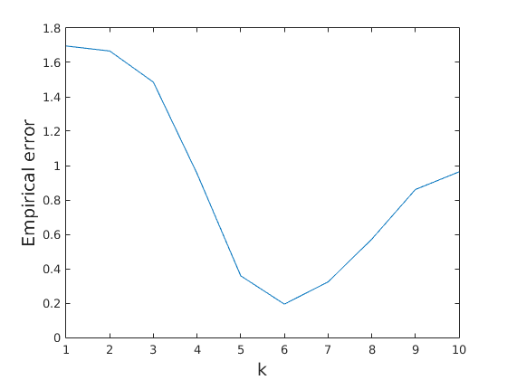
Fig. 5.4: The empirical error $\|u_{0}-u_{h}\|_{n}$ for 11 different choices of $\lambda_{n}=10^{-k},k=0,1,\cdots,10$. The mesh size $h=\lambda_{n}^{1/4}$.

Example 5.2.

In this example we show the empirical error $\|u_{0}-u_{h}\|_{n}$ depends linearly on $\lambda_{n}^{1/2}$ to confirm (4.20). We set $e_{i},~{}i=1,2,\cdots,n$, to be independent normal random variables with variance $\sigma=1$. We take $n$ varying from $2500$ to $9\times 10^{4}$. In this test we use the optimal $\lambda_{n}$ and take the mesh size $h=\lambda^{1/4}_{n}$. Figure 5.5 (a) shows clearly the linear dependence of the empirical error on $\lambda_{n}^{1/2}$. We also run the test for combined random errors, i.e., $e_{i}=\eta_{i}+\alpha_{i}$, where $\eta_{i}$ and $\alpha_{i}$ are independent normal random variables with variance $\sigma_{1}=1$ and $\sigma_{2}=10$. Figure 5.5 (b) shows also the linear dependence of the empirical error on $\lambda_{n}^{1/2}$.

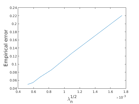
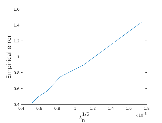
(a)	(b)

Fig. 5.5: (a) The linear dependence of the empirical error $\|u_{0}-u_{h}\|_{n}$ on $\lambda_{n}^{1/2}$ for $\sigma=1$. (b) The linear dependence of the empirical error $\|u_{0}-u_{h}\|_{n}$ on $\lambda_{n}^{1/2}$ for combined random noises.

Example 5.3.

We test the efficiency of the Algorithm 5.1 to estimate the smoothing parameter $\lambda_{n}$. We will show two experiments of different noise levels. In the first test we set $e_{i},~{}i=1,2,\cdots,n$, being independent normal random variables with variance $\sigma=1$ and $n=2500$. Figure 5.6 (a) and (b) show clearly that the sequence of $\{\lambda_{n,k}\}$ generated by Algorithm 5.1 converges. $\lambda_{n,16}=4.12\times 10^{-6}$ agrees with the optimal choice $3\times 10^{-6}$ given by (4.19). Furthermore, $\|u_{h}-y\|_{n}=0.99$ provides a good estimate of the variance $\sigma$.

We now consider the combined random noise. Let $e_{i}=\eta_{i}+\alpha_{i},~{}i=1,2,\cdots,n$, where $\eta_{i}$ and $\alpha_{i}$ are independent normal random variables with variance $\sigma_{1}=1$ and $\sigma_{2}=10$. It is obvious that $\sigma^{2}={\mathbb{E}}e_{i}^{2}=\sigma_{1}^{2}+\sigma_{2}^{2}=101$. Let $n=4\times 10^{4}$. Again Figure 5.6 (c) and (d) show the sequence $\{\lambda_{n,k}\}$ generated by Algorithm 5.1 converges. Now $\lambda_{n,19}=2.16\times 10^{-5}$ which fits well the optimal choice $1.03\times 10^{-5}$ given by (4.19). Also $\|u_{h}-y\|_{n}=10.07$ gives a good estimate of the variance $\sigma$.

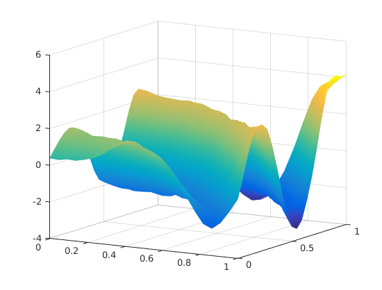
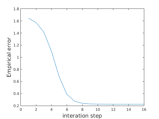
(a)	(b)
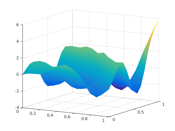
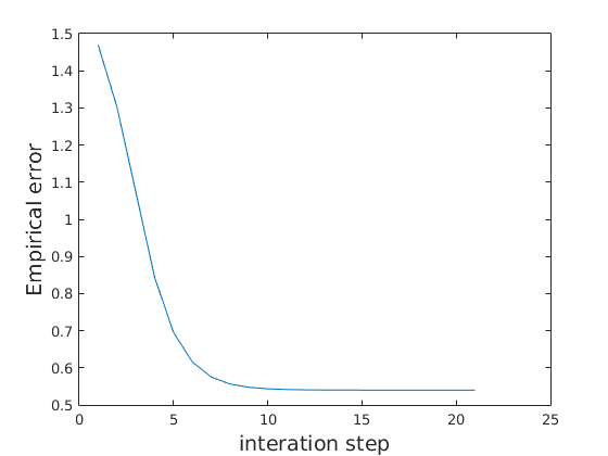
(c)	(d)

Fig. 5.6: (a) The solution $u_{h}$ at the end of iteration for $\sigma=1$. (b) The empirical error $\|u_{0}-u_{h}\|_{n}$ of each iteration for $\sigma=1$. (c) The solution $u_{h}$ at the end of iteration for the combined random error $e_{i}=\eta_{i}+\alpha_{i}$. (d) The empirical error $\|u_{0}-u_{h}\|_{n}$ of each iteration for the combined random error $e_{i}=\eta_{i}+\alpha_{i}$.

6 Appendix: Proof of Lemma 3.5 when $d=3$

The proof is very similar to the proof for 2D case in section 3. We will construct $\Pi_{h}v_{h}$ by using the three dimensional $C^{1}$ element of Zhang constructed in [13] which simplifies an earlier construction of Zenisek [14]. For any tetrahedron $K\in{\cal M}_{h}$, the $C^{1}-P_{9}$ element in [13] is a triple $(K,P_{K},\Lambda_{K})$, where $P_{K}=P_{9}(K)$ and the set of degrees of freedom $\Lambda_{K}$ consists of the following $220$ functionals: for any $p\in C^{2}(K)$,

$1^{\circ}$

The nodal values of $p(a_{i}),Dp(a_{i})(a_{j}-a_{i}),D^{2}p(a_{i})(a_{j}-a_{i},a_{k}-a_{i}),D^{3}(a_{i})(a_{j}-a_{i},a_{k}-a_{i},a_{l}-a_{i}),D^{4}p(a_{i})(a_{j}-a_{i},a_{k}-a_{i},a_{l}-a_{i},a_{n}-a_{i}),1\leq i\leq 4,1\leq j\leq k\leq l\leq n\leq 4,i\not\in\{j,k,l,n\}$, where $\{a_{i}\}^{4}_{i=1}$ are the vertices of $K$; (120 functionals)

$2^{\circ}$

The 2 first order normal derivatives $\partial_{\nu_{k}}p(a_{ij})$ and 3 second order normal derivatives $\partial^{2}_{\nu_{k}\nu_{l}}p(b_{ij}),\partial^{2}_{\nu_{k}\nu_{l}}p(c_{ij})$ on the edge with vertices $a_{i},a_{j}$, $1\leq i\not=j\leq 4$, where $\nu_{k},k=1,2,$ are unit vectors perpendicular to the edge, and $a_{ij}=(a_{i}+a_{j})/2$, $b_{ij}=(2a_{i}+a_{j})/3$, $c_{ij}=(a_{i}+2a_{j})/3$; (48 functionals)

$3^{\circ}$

The nodal value $p(a_{ijk})$ and 6 normal derivatives $\partial_{\nu}p(a_{ijk}^{n})$ on the face with vertices $a_{i},a_{j},a_{k}$, $1\leq i,j,k\leq 4,i\not=j,j\not=k,k\not=i$, $n=1,2,\cdots,6$, where $a_{ijk}$ is the barycenter of the face and $a_{ijk}^{1}=(2a_{i}+a_{j}+a_{k})/4,a_{ijk}^{2}=(a_{i}+2a_{j}+a_{k})/4,a_{ijk}^{3}=(a_{i}+a_{j}+2a_{k})/4,a_{ijk}^{4}=(4a_{i}+a_{j}+a_{k})/6,a_{ijk}^{5}=(a_{i}+4a_{j}+a_{k})/6,a_{ijk}^{6}=(a_{i}+a_{j}+4a_{k})/6$; (24 functionals)

$4^{\circ}$

The nodal values $p(d_{i})$, $1\leq i\leq 4$, at internal points $d_{1}=(2a_{1}+a_{2}+a_{3}+a_{4})/5,d_{2}=(a_{1}+2a_{2}+a_{3}+a_{4})/5,d_{3}=(a_{1}+a_{2}+2a_{3}+a_{4})/5,d_{4}=(a_{1}+a_{2}+a_{3}+2a_{4})/5$. (4 functionals)

Let $X_{h}$ be the finite element space

$$X_{h}=\{v_{h}:v_{h}|_{K}\in P_{9}(K),\forall K\in{\cal M}_{h},f(v_{h}|_{K_{1}})=f(v_{h}|_{K_{2}}),\forall f\in\Lambda_{K_{1}}\cap\Lambda_{K_{2}}\}.$$

It is known that $X_{h}\subset H^{2}(\Omega)$. We define the operator $\Pi_{h}$ as follows. For any $v_{h}\in V_{h}$, $w_{h}:=\Pi_{h}v_{h}\in X_{h}$ such that for any $K\in{\cal M}_{h}$, $w_{h}|_{K}\in P_{9}(K)$, for the degrees of freedom at vertices $a_{i}$, $1\leq i\leq 4$,

$$\partial^{\alpha}(w_{h}|_{K})(a_{i})=\frac{1}{N(a_{i})}\sum_{K^{\prime}\in{\cal M}_{h}(a_{i})}\partial^{\alpha}(v_{h}|_{K^{\prime}})(a_{i}),\ \ |\alpha|\leq 4,$$ (6.1)

for the degrees of freedom on the edge with vertices $a_{i},a_{j}$, $1\leq i\not=j\leq 4$,

$$\partial_{\nu_{k}}(w_{h}|_{K})(a_{ij})=\frac{1}{N(a_{ij})}\sum_{K^{\prime}\in{\cal M}_{h}(a_{ij})}\partial_{\nu_{k}}(v_{h}|_{K^{\prime}})(a_{ij}),\ \ k=1,2,$$ (6.2)

$$\partial_{\nu_{k}\nu_{l}}(w_{h}|_{K})(b_{ij})=\frac{1}{N(b_{ij})}\sum_{K^{\prime}\in{\cal M}_{h}(b_{ij})}\partial_{\nu_{k}\nu_{l}}(v_{h}|_{K^{\prime}})(b_{ij}),\ \ k,l=1,2,$$ (6.3)

$$\partial_{\nu_{k}\nu_{l}}(w_{h}|_{K})(c_{ij})=\frac{1}{N(c_{ij})}\sum_{K^{\prime}\in{\cal M}_{h}(c_{ij})}\partial_{\nu_{k}\nu_{l}}(v_{h}|_{K^{\prime}})(c_{ij}),\ \ k,l=1,2,$$ (6.4)

for the degrees of freedom on the faces with vertices $a_{i},a_{j},a_{k}$, $1\leq i,j,k\leq 4,i\not=j,j\not=k,k\not=i$,

$$(w_{h}|_{K})(a_{ijk})=\frac{1}{N(a_{ijk})}\sum_{K^{\prime}\in{\cal M}_{h}(a_{ijk})}(v_{h}|_{K^{\prime}})(a_{ijk}),$$ (6.5)

$$\partial_{\nu}(w_{h}|_{K})(a_{ijk}^{n})=\frac{1}{N(a_{ijk}^{n})}\sum_{K^{\prime}\in{\cal M}_{h}(a_{ijk}^{n})}\partial_{\nu}(v_{h}|_{K^{\prime}})(a_{ijk}^{n}),\ \ n=1,2\,\cdots,6,\$$ (6.6)

and finally for the degrees of freedom at the interior points $d_{i},1\leq i\leq 4$,

$$(w_{h}|_{K})(d_{i})=(v_{h}|_{K})(d_{i}).$$ (6.7)

To show the desired estimate (3.6) in 3D we use the $C^{0}$-$P_{9}$ element in [13] which is a triple $(K,P_{K},\Theta_{K})$, where $P_{K}=P_{9}(K)$ and the set of degrees of freedom $\Theta_{K}$ is defined by replacing some of the degrees of freedom of the $C^{1}-P_{9}$ element $\Lambda_{K}$ as follows:

$1^{\circ}$

For the edge with vertices $a_{i},a_{j}$, $1\leq i\not=j\leq 4$, replace the 2 edge first order normal derivatives by $Dp(a_{ij})(a_{k}-a_{ij}),Dp(a_{ij})(a_{l}-a_{ij})$ and denote the corresponding nodal basis functions $p_{ij}^{k}(x),p_{ij}^{l}(x)$, where $a_{k},a_{l}$ are the other 2 vertices of $K$ other than $a_{i},a_{j}$;

$2^{\circ}$

For the edge with vertices $a_{i},a_{j}$, $1\leq i\not=j\leq 4$, replace the 3 edge second order normal derivatives by $D^{2}p(b_{ij})(a_{k}-b_{ij},a_{l}-b_{ij}),D^{2}p(c_{ij})(a_{k}-b_{ij},a_{l}-b_{ij})$ and denote the corresponding nodal basis functions $p_{ij}^{kl}(x),q_{ij}^{kl}(x)$, where $a_{k},a_{l}$ are the other 2 vertices of $K$ other than $a_{i},a_{j}$;

$3^{\circ}$

For the face with vertices $a_{i},a_{j},a_{k}$, $1\leq i,j,k\leq 4,i\not=j,j\not=k,k\not=i$, replace the face normal derivatives by $Dp(a_{ijk}^{n})(a_{l}-a_{ijk}^{n})$ and denote the corresponding nodal basis functions $p_{ijk}^{n}(x)$, where $a_{l}$ is the vertex of $K$ other than $a_{i},a_{j},a_{k}$, $n=1,2\cdots,6$.

A regular family of this $C^{0}-P_{9}$ element is affine-equivalent. For any $v_{h}\in V_{h}$, we also define an operator $q_{h}:=\Lambda_{h}v_{h}$ in a similar way as the definition of $\Pi_{h}$ by replacing the average normal derivatives in (6.2)-(6.4) and (6.6) by the corresponding directional derivatives in the definition of degrees of freedom for the $C^{0}-P_{9}$ element. By the same argument as that in the proof of 2D case in section 3 we have

$$|v_{h}-q_{h}|_{H^{m}(K)}\leq Ch^{2-m}\left(\sum_{K^{\prime}\in{\cal M}_{h}(K)}|v_{h}|_{H^{2}(K^{\prime})}^{2}\right)^{1/2},\ \ m=0,1,2.$$ (6.8)

Next we expend $q_{h}-w_{h}\in P_{9}(K)$ in terms of the nodal basis functions of the $C^{0}-P_{9}$ element. From the definition of the $C^{1}-P_{9}$ and $C^{0}-P_{9}$ elements, we have $q_{h}-w_{h}=\phi_{e}+\phi_{f}$ in $K$, where the edge part of the function $q_{h}-w_{h}$ is

$$\phi_{e}(x) = \sum_{\stackrel{{\scriptstyle 1\leq i\not=j\leq 4}}{{\{k,l\}\in\{1,2,3,4\}\backslash\{i,j\},k\not=l}}}\Big{[}D(q_{h}|_{K}-w_{h}|_{K})(a_{ij})(a_{k}-a_{ij})p_{ij}^{k}(x)$$

$$\hskip 85.35826pt+\ D(q_{h}|_{K}-w_{h}|_{K})(a_{ij})(a_{l}-a_{ij})p_{ij}^{l}(x)\Big{]}$$

$$+\sum_{\stackrel{{\scriptstyle 1\leq i\not=j\leq 4}}{{\{k,l\}\in\{1,2,3,4\}\backslash\{i,j\},k\leq l}}}\Big{[}D^{2}(q_{h}|_{K}-w_{h}|_{K})(b_{ij})(a_{k}-b_{ij},a_{l}-b_{ij})p_{ij}^{kl}(x)$$

$$\hskip 85.35826pt+\ D^{2}(q_{h}|_{K}-w_{h}|_{K})(c_{ij})(a_{k}-c_{ij},a_{l}-c_{ij})q_{ij}^{kl}(x)\Big{]},$$

and the face part of the function $q_{h}-w_{h}$ is

$$\phi_{f}(x)=\sum_{\stackrel{{\scriptstyle 1\leq i,j,k\leq 4,i\not=j,j\not=k,k\not=i}}{{\{l\}\in\{1,2,3,4\}\backslash\{i,j,k\}}}}\sum^{6}_{n=1}D(q_{h}|_{K}-w_{h}|_{K})(a_{ijk}^{n})(a_{l}-a_{ijk}^{n})p_{ijk}^{n}(x).$$

Since the tangential derivatives of $q_{h}-w_{h}$ along the edges vanish, we obtain by the same argument as that in the proof of 2D case in section 3 that

$$|\phi_{e}|_{H^{m}(K)}\leq Ch^{2-m}\left(\sum_{K^{\prime}\in{\cal M}_{h}(K)}|v_{h}|_{H^{2}(K^{\prime})}^{2}\right)^{1/2},\ \ m=0,1,2.$$ (6.9)

On any face $F$ of $K$, $q_{h}-w_{h}-\phi_{e}\in P_{9}(F)$ and its nodal values at 3 vertices up to 4th order derivatives vanish, its first order normal derivative at the midpoint and two second order normal derivatives at two internal trisection points on 3 edges vanish, and the nodal value at the barycenter also vanishes. This implies $q_{h}-w_{h}-\phi_{e}=0$ on any face of the element $K$. Let $\tau_{ijk}^{n}$ be the tangential unit vector on the face of vertices $a_{i},a_{j},a_{k}$ such that

$$a_{l}-a_{ijk}^{n}=[(a_{l}-a_{ijk}^{n})\cdot\tau_{ijk}^{n}]\tau^{n}_{ijk}+[(a_{l}-a_{ijk}^{n})\cdot\nu]\nu.$$

Now by (6.4), (6.8)-(6.9), and the inverse estimate we have

$$|D(q_{h}|_{K}-w_{h}|_{K})(a_{ijk}^{n})(a_{l}-a_{ijk}^{n})|$$ (6.10)

$$\leq |[(a_{l}-a_{ijk}^{n})\cdot\tau_{ijk}^{n}]D\phi_{e}(a_{ijk}^{n})\tau_{ijk}^{n}|+|[(a_{l}-a_{ijk}^{n})\cdot\nu]D(q_{h}|_{K}-w_{h}|_{K})(a_{ijk}^{n})\nu|$$

$$\leq Ch^{1/2}\left(\sum_{K^{\prime}\in{\cal M}_{h}(K)}|v_{h}|_{h^{2}(K^{\prime})}^{2}\right)^{1/2}.$$

Since a regular family of $C^{0}-P_{9}$ element is affine-equivalent, we have $|p_{ijk}^{n}|_{H^{m}(K)}\leq Ch^{3/2-m}$, $m=0,1,2$. Therefore, by (6.10) we obtain

$$|\phi_{f}|_{H^{m}(K)}\leq Ch^{2-m}\left(\sum_{K^{\prime}\in{\cal M}_{h}(K)}|v_{h}|_{H^{2}(K^{\prime})}^{2}\right)^{1/2},\ \ m=0,1,2.$$ (6.11)

Combining (6.8), (6.9), (6.11) yields the desired estimate (3.6) in 3D since $v_{h}-w_{h}=(v_{h}-q_{h})+\phi_{e}+\phi_{f}$ in $K$. The estimate (3.7) can be proved in the same way as the proof for the 2D case in section 3. This completes the proof. $\Box$

References

- [1] R. Arcangéli, R. Manzanilla, and J.J. Torrens, Approximation spline de surfaces de type explicite comportant des failles, Math. Model. Numer. Anal. 31 (1997), pp. 643-676.
- [2] M.S. Birman and M.Z. Solomyak, Piecewise polynomial approximations of functions of the classes , Mat. Sb. 73 (1967), pp. 331-355.
- [3] P.G. Ciarlet, The Finite Element Method for Elliptic Problems, North-Holland, Amsterdam, 1978.
- [4] J. Duchon, Splines minimizing rotation-invariant semi-norms in Sobolev spaces, in Constructive Theory of Functions of Several Variables, Lecture Notes in Mathematics 571, 1977, pp. 85-100.
- [5] L.S.D. Morley, The triangular equilibrium element in the solution of plate bending problems, Aero. Quart. 19 (1968), pp. 149-169.
- [6] S. Roberts, M. Hegland, and I. Altas, Approximation of a thin plate spline smoother using continuous piecewise polynomial functions, SIAM J. Numer. Anal. 41 (2003), pp. 208-234.
- [7] Z.-C. Shi, On the error estimates of Morley element, Numerica Mathematica Sinica 12 (1990), pp. 113-118. (in Chinese)
- [8] F.I. Utreras, Convergence rates for multivariate smoothing spline functions, J. Approx.Theory 52 (1988), pp. 1-27.
- [9] M. Wang and J. Xu, The Morley element for fourth order elliptic equations in any dimensions, Numer. Math. 103 (2006), pp. 155-169.
- [10] S.A. van de Geer, Empirical process in M-estimation, Cambridge University Press, Cambridge, 2000.
- [11] A.W. van der Vaart and J.A. Wellner, Weak Convergence and Empirical Processes: with Applications to Statistics, Springer, New York, 1996.
- [12] G. Wahba, Spline Models for Observational Data, SIAM, Philadelphia, 1990.
- [13] S. Zhang, A family of 3D continuously differentiable finite elements on tetrahedral grids, Appl. Numer. Math. 59 (2009), pp. 219-233.
- [14] A. Zenisek, Alexander polynomial approximation on tetrahedrons in the finite element method, J. Approx. Theory 7 (1973), pp. 334-351.