Extracting three-body breakup observables from CDCC calculations with core excitations

Abstract

Background

Core-excitation effects in the scattering of two-body halo nuclei have been investigated in previous works. In particular, these effects have been found to affect in a significant way the breakup cross sections of neutron-halo nuclei with a deformed core. To account for these effects, appropriate extensions of the continuum-discretized coupled-channels (CDCC) method have been recently proposed.

Purpose

We aim to extend these studies to the case of breakup reactions measured under complete kinematics or semi-inclusive reactions in which only the angular or energy distribution of one of the outgoing fragments is measured.

Method

We use the standard CDCC method as well as its extended version with core excitations (XCDCC), assuming a pseudo-state basis for describing the projectile states. Two- and three-body observables are computed by projecting the discrete two-body breakup amplitudes, obtained within these reaction frameworks, onto two-body scattering states with definite relative momentum of the outgoing fragments and a definite state of the core nucleus.

Results

Our working example is the one-neutron halo ¹¹Be. Breakup reactions on protons and ⁶⁴Zn targets are studied at 63.7 MeV/nucleon and 28.7 MeV, respectively. These energies, for which experimental data exist, and the targets provide two different scenarios where the angular and energy distributions of the fragments are computed. The importance of core dynamical effects is also compared for both cases.

Conclusions

The presented method provides a tool to compute double and triple differential cross sections for outgoing fragments following the breakup of a two-body projectile, and might be useful to analyze breakup reactions with other deformed weakly-bound nuclei, for which core excitations are expected to play a role. We have found that, while dynamical core excitations are important for the proton target at intermediate energies, they are very small for the Zn target at energies around the Coulomb barrier.

I Introduction

Recent experimental activities with nuclei in the proximity of the drip-lines have increased the interest in this region of the nuclear landscape. In particular, special attention has been paid to halo nuclei, spatial extended quantum systems with one or two loosely bound valence particles, for example ¹¹Be or ¹¹Li. Breakup reactions have shown to be a useful tool for extracting information from these exotic structures Nakamura and Kondo (2012). Reliable and well understood few-body reaction frameworks to describe breakup reactions of exotic nuclei, such as haloes, are therefore needed. Particularly, it is timely to estimate what are the relevant excitations mechanisms for the reaction. In the case of elastic breakup, that we address here, several few-body formalisms have been developed to extract the corresponding cross sections: Continuum-Discretized Coupled-Channels (CDCC) method Rawitscher (1974); Austern et al. (1987), the adiabatic approximation Banerjee and Shyam (2000); Tostevin et al. (1998), the Faddeev/AGS equations Faddeev (1960); Alt et al. (1967), and a variety of semiclassical approximations Typel and Baur (1994); Esbensen and Bertsch (1996); Kido et al. (1994); Typel and Baur (2001); Capel et al. (2004); García-Camacho et al. (2006). The CDCC method is based upon an explicit discretization of all channels in the continuum and requires the solution of an extensive set of coupling equations. It has been applied at both low and intermediate energies.

The standard formulation of these approaches ignore the possible excitations of the constituent fragments: the states of the few-body system are usually described by pure single-particle configurations, ignoring the admixtures of different core states in the wave functions of the projectile. These admixtures are known to be important, particularly in the case of well-deformed nuclei, such as the ¹¹Be halo nucleus Lay et al. (2012). In addition, for such two-body weakly bound system, dynamic core excitation effects in breakup have been recently studied with an extension of the Distorted Wave Born Approximation (DWBA) formalism within a no-recoil approximation Crespo et al. (2011); Moro and Crespo (2012); Moro and Lay (2012); Moro et al. (2012) and found to be important. This method is based in the Born approximation and ignores higher order effects (such as continuum-continuum couplings). A recent attempt to incorporate core excitation effects within a coupled-channels calculation was done in Ref. de Diego et al. (2014), using an extended version of the CDCC formalism Summers et al. (2006), hereafter referred to as XCDCC. The different calculations have shown that, for light targets, dynamic core excitations give rise to sizable changes in the magnitude of the breakup cross sections. Additionally, these excitations have been found to be dominant in resonant breakup of ¹⁹C on a proton target Lay et al. (2016). These effects have also been studied within the Faddeev/AGS approach in the analysis of breakup and transfer reactions Crespo et al. (2011); Deltuva (2015); Deltuva et al. (2016).

Within the CDCC and XCDCC reaction formalisms, the breakup is treated as an excitation of the projectile to the continuum so the theoretical cross sections are described in terms of the c.m. scattering angle of the projectile and the relative energy of the constituents, using two-body kinematics. Because of this, experimental data should be transformed to the c.m. frame for comparison, but this process is ambiguous in the case of inclusive data. This is a common situation, for example, in the case of reactions involving neutron-halo nuclei in which very often only the charged fragments are detected. Furthermore, even in exclusive breakup experiments under complete kinematics, in which this transformation is feasible, the possibility of comparing the calculated and experimental cross sections for different configurations (angular and energy) of the outgoing fragments provides a much deeper insight of the underlying processes, as demonstrated by previous analyses performed by exclusive breakup measurements with stable nuclei Aarts et al. (1984). The continuous developments at the radioactive beam facilities opens the exciting possibility of extending these studies to unstable nuclei. This will require improvements and extensions of existing formalisms to provide these observables.

In the case of the CDCC framework, fivefold fully exclusive cross sections were already derived in Tostevin et al. (2001). In the present work we extend this framework to the XCDCC formalism and we provide more insight into the contribution of core admixtures (CA) and dynamic core excitation (DCE) in the collision process. A proper inclusion of core excitation effects in the description of kinematically fully exclusive observables in the laboratory frame is the primary motivation of this manuscript with the aim of pinning down the effect of this degree of freedom in angular and energy distributions. Additionaly, this allows to compute breakup observables for specific states of the core nucleus, which could be of utility in experiments using gamma rays coincidences. The calculations are carried out within the combined XCDCC+THO framework de Diego et al. (2014) for breakup reactions of ¹¹Be on protons and ⁶⁴Zn targets with full three-body kinematics. The formalism is applied to investigate the angular and energy distributions of the ¹⁰Be fragments resulting from the breakup, for which new measurements have been made Di Pietro et al. (2010).

The paper is organized as follows. In Sec. II we briefly discuss the structure approach to describe two-body loosely-bound systems with core excitation. In Sec. III, the expression of the scattering wave functions is derived. The three-body breakup amplitudes are shown in Sec. IV and the related most exclusive observables are presented in Sec. V. In Sec. VI, we show some working examples. We study ¹¹Be+$p$ and ¹¹Be+⁶⁴Zn reactions at low energies and we calculate the angular and energy distributions of the ¹⁰Be fragments after the breakup. In Sec. VII, the main results and remarks of this work are collected.

II The Structure formalism

In this manuscript, the composite projectile is assumed to be well described by a valence nucleon coupled to a core nucleus and the projectile states are described in the weak-coupling limit. Thus, these states are expanded as a superposition of products of single-particle configurations and core states. The energies and wavefunctions of the projectile are calculated using the pseudo-state (PS) method Matsumoto et al. (2003), that is, diagonalizing the model Hamiltonian in a basis of square-integrable functions. For the relative motion between the valence particle and the core, we use a recently proposed extension of the analytical Transformed Harmonic Oscillator (THO) basis Lay et al. (2012), which incorporates the possible excitations of the constituents of the composite system. This approach differs from the binning procedure Tostevin et al. (2001), where the continuum spectrum is represented by a set of wave packets, constructed as a superposition of scattering states calculated by direct integration of the multi-channel Schrödinger equation. The main advantage of the PS method relies on the fact that it provides a suitable representation of the continuum spectrum with a reduced number of functions and, as we will see below, it is particularly convenient to describe narrow resonances.

We briefly review the features of the PS basis used in this work to describe the states of the two-body composite projectile. The full Hamiltonian, under the weak-coupling limit, would be written as:

$$H=\hat{T}_{r}+V_{cv}({\mathbf{r}},\xi)+H_{\rm core}(\xi),$$ (1)

where $\hat{T}_{r}$ (kinetic energy) and $V_{cv}({\mathbf{r}},\xi)$ (effective potential) describe the relative motion between the core and the valence while $H_{\rm core}(\xi)$ is the intrinsic hamiltonian of the core, whose internal degrees of freedom are described through the coordinate $\xi$. The eigenstates of $H_{\rm core}(\xi)$ corresponding to energies $\epsilon_{I}$ (defined by the intrinsic spin of the core, $I$) will be denoted by $\phi_{I}$ and, additional quantum numbers, required to fully specify the core states, will be given below.

The core-valence interaction is assumed to contain a noncentral part, responsible for the CA in the projectile states. In general, this potential can be expanded into multipoles:

$$V_{cv}({\mathbf{r}},\xi)=\sum_{\lambda\mu}V_{\lambda\mu}(r,\xi)Y_{\lambda\mu}(\hat{r}).$$ (2)

In this work the projectile is treated within the particle-rotor model Bohr and Mottelson (1969) with a permanent core deformation (assumed to be axially symmetric). Thus, in the body-fixed frame, the surface radius is parameterized in terms of the deformation parameter, $\beta_{2}$, as $R(\hat{\xi})=R_{0}[1+\beta_{2}\,Y_{20}(\hat{\xi})]$, with $R_{0}$ an average radius. The full valence-core interaction is obtained by deforming a central potential $V^{(0)}_{cv}(r)$ as follows,

$$V_{cv}({\mathbf{r}},\hat{\xi})=V_{cv}^{(0)}\left(r-\delta_{2}Y_{20}(\hat{\xi})\right),$$ (3)

where $\delta_{2}=\beta_{2}R_{0}$ is the so-called deformation length. The transformation to the space-fixed reference frame is made through the rotation matrices ${\cal D}^{\lambda}_{\mu 0}(\alpha,\beta,\gamma)$ (depending on the Euler angles $\{\alpha,\beta,\gamma\}$). After expanding in spherical harmonics (see e.g. Ref. Tamura (1965)), the potential in Eq. (3) reads

$$V_{cv}({\mathbf{r}},\hat{\xi})=\sqrt{4\pi}\sum_{\lambda\mu}{\cal V}^{\lambda}_{cv}(r){\cal D}^{\lambda}_{\mu 0}(\alpha,\beta,\gamma)Y_{\lambda\mu}(\hat{r}),$$ (4)

with the radial form factors ($u=\cos\theta^{\prime}$):

$${\cal V}^{\lambda}_{cv}(r)=\frac{\sqrt{2\lambda+1}}{2}\int_{-1}^{1}V_{cv}\left(r-\delta_{2}Y_{20}(\theta^{\prime},0)\right)P_{\lambda}(u)~{}{\mathrm{d}}u.$$ (5)

In comparison with Eq. (2) we have for a particle-rotor model:

$$V_{\lambda\mu}^{rotor}(r,\hat{\xi})=\sqrt{4\pi}{\cal V}^{\lambda}_{cv}(r){\cal D}^{\lambda}_{\mu 0}(\alpha,\beta,\gamma).$$ (6)

The eigenstates of the Hamiltonian (1) will be a superposition of several valence configurations and core states $\alpha=\{\ell,s,j,I\}$, with $\vec{\ell}$ (valence-core orbital angular momentum) and $\vec{s}$ (spin of the valence) both coupled to $\vec{j}$ (total valence particle angular momentum), for a given total angular momentum and parity of the composite projectile, $J^{\pi}$ , i.e.:

$$\Psi_{\varepsilon,J,M}({\mathbf{r}},\xi)=\sum_{\alpha}^{n_{\alpha}}\frac{R^{J}_{\varepsilon,\alpha}(r)}{r}\Phi_{\alpha,J,M}(\hat{r},\xi_{v},\xi_{c}),$$ (7)

where $n_{\alpha}$ is the number of such channel configurations and the set of functions

$$\Phi_{\alpha,J,M}(\hat{r},\xi_{v},\xi_{c})\equiv\left[{\cal Y}_{\ell sj}(\hat{r})\otimes\phi_{I}(\xi)\right]_{JM}$$ (8)

is the so-called spin-orbit basis.

The functions $R^{J}_{\varepsilon,\alpha}(r)$ are here obtained by diagonalizing the Hamiltonian in a basis of square-integrable states, such as the THO basis. For each channel $\alpha$, we consider a set of $N$ functions $R^{THO}_{n,\alpha}(r)$ (with $n=1,\ldots,N$). The eigenvectors of the Hamiltonian will be of the form:

$$\Psi^{(N)}_{i,J,M}({\mathbf{r}},\xi)=\sum_{\alpha}^{n_{\alpha}}\sum_{n=1}^{N}c^{i}_{n,\alpha,J}\frac{R^{THO}_{n,\alpha}(r)}{r}\Phi_{\alpha,J,M}(\hat{r},\xi_{v},\xi_{c}),$$ (9)

where $i$ is an index that identifies each eigenstate and $c^{i}_{n,\alpha,J}$ are the corresponding expansion coefficients in the truncated basis, obtained by diagonalization of the full Hamiltonian (1).

For numerical applications, the sum over the index of the THO basis can be actually performed to get

$$\Psi^{(N)}_{i,J,M}({\mathbf{r}},\xi_{v},\xi_{c})=\sum_{\alpha}\frac{g_{i,\alpha}^{J}(r)}{r}\Phi_{\alpha,J,M}(\hat{r},\xi_{v},\xi_{c})$$ (10)

where the radial function is:

$$g_{i,\alpha}^{J}(r)=\sum_{n=1}^{N}c^{i}_{n,\alpha,J}R^{THO}_{n,\alpha}(r).$$ (11)

The negative eigenvalues of the Hamiltonian (1) are identified with the energies of bound states whereas the positive ones correspond to a discrete representation of the continuum spectrum.

III Scattering wave functions

For the calculation of the three-body scattering observables (see Sec. IV) we need also the exact scattering states of the valence+core system for a given asymptotic relative wave vector $\bm{k}_{I}$, and given spins of the core ($I$) and valence particle ($s$), as well as their respective projections ($\mu$ and $\sigma$, respectively), that will be denoted as $\phi_{{\mathbf{k}}_{I};I\mu;s\sigma}^{(+)}({\mathbf{r}},\xi_{v},\xi_{c})$. These states can be written as a linear combination of the continuum states with good angular momentum $J,M$, that are of the form

$$\Psi^{(+)}_{\alpha,J,M}(k_{I},{\mathbf{r}},\xi_{v},\xi_{c})=\sum_{\alpha^{\prime}}\frac{f^{J}_{\alpha:\alpha^{\prime}}(k_{I},r)}{r}\Phi_{\alpha^{\prime},J,M}(\hat{r},\xi_{v},\xi_{c}),$$ (12)

where the radial functions $f^{J}_{\alpha:\alpha^{\prime}}(k_{I},r)$ are the solution of the coupled differential equations,

$$\left[E_{\alpha^{\prime}}-T_{r\ell^{\prime}}-V^{J}_{\alpha^{\prime}:\alpha^{\prime}}\right]f^{J}_{\alpha:\alpha^{\prime}}(k_{I},r)=$$

$$\sum_{\alpha^{\prime\prime}\neq\alpha^{\prime}}V^{J}_{{\alpha^{\prime}:\alpha^{\prime\prime}}}f^{J}_{\alpha:\alpha^{\prime\prime}}(k_{I},r),$$ (13)

where $E_{\alpha^{\prime}}=E_{\alpha}-\epsilon_{I^{\prime}}+\epsilon_{I}$, as a consequence of the energy conservation in the nucleon-core system when the latter is in the state $I$ or $I^{\prime}$, $T_{r\ell^{\prime}}$ is the relative kinetic energy operator, and $V^{J}_{{\alpha^{\prime}:\alpha^{\prime\prime}}}$ are the coupling potentials given by

$$V^{J}_{{\alpha^{\prime}:\alpha^{\prime\prime}}}(r)=\langle\alpha^{\prime}JM|V_{vc}|\alpha^{\prime\prime}JM\rangle$$ (14)

with $|\alpha^{\prime}JM\rangle$ denoting the spin-basis defined in Eq. (8).

These radial functions behave asymptotically as a plane wave in a given incoming channel $\alpha$ and outgoing waves in all channels, i.e.:

$$f^{J}_{\alpha:\alpha^{\prime}}(k_{I},r)\rightarrow e^{i\sigma_{\ell}}\left[F_{\ell}(k_{I}r)\delta_{\ell,\ell^{\prime}}+T^{J}_{\alpha,\alpha^{\prime}}H^{(+)}_{\ell^{\prime}}(k_{I}r)\right],$$ (15)

where $\sigma_{\ell}$ are the Coulomb phase shifts, $F_{\ell}(k_{I}r)$ the regular Coulomb function and $T^{J}_{\alpha,\alpha^{\prime}}$ the T-matrix, that is directly related to the S-matrix according to:

$$S^{J}_{\alpha,\alpha^{\prime}}=\delta_{\alpha,\alpha^{\prime}}+2iT^{J}_{\alpha,\alpha^{\prime}}.$$ (16)

In terms of these good-angular momentum states, the scattering states result (see Appendix A)

$$\phi_{{\mathbf{k}}_{I};I\mu;s\sigma}^{(+)}({\mathbf{r}},\xi_{v},\xi_{c})= \frac{4\pi}{k_{I}r}\sum_{\ell,j,J,M}i^{\ell}Y^{*}_{\ell m}(\hat{k_{I}})\langle\ell ms\sigma|jm_{j}\rangle\langle jm_{j}I\mu|JM\rangle\sum_{\alpha^{\prime}}f^{J}_{\alpha:\alpha^{\prime}}(k_{I},r)\Phi_{\alpha^{\prime},J,M}(\hat{r},\xi_{v},\xi_{c}),$$ (17)

where $m_{j}=M-\mu$, and $m=m_{j}-\sigma$.

IV Breakup amplitudes

The scattering problem can be described by means of the breakup transition amplitude $T_{\mu\sigma;M_{0}}^{Is;J_{0}}(\bm{k}_{I},\bm{K})$ connecting an initial state $|J_{0}M_{0}\rangle$ with a three-body final state comprised by the target (assumed to be structureless), the valence particle and the core, whose motion is described in terms of the relative momentum, $\bm{k}_{I}$, and a c.m. wave vector, $\bm{K}$, that differs from the initial momentum, $\bm{K}_{0}$, in $|J_{0}M_{0}\rangle$.

We proceed to relate $T_{\mu\sigma;M_{0}}^{Is;J_{0}}$ to the discrete XCDCC two-body inelastic amplitudes $T_{M_{0},M^{\prime}}^{i,J_{0},J^{\prime}}(\theta_{i},K_{i})$, obtained after solving the coupled equations in the XCDCC method and evaluated on the discrete values of $\bm{K}$, given by the $\{\bm{K}_{i}\}=\{\theta_{i},K_{i}\}$ grid. In order to obtain this relationship, we replace the exact three-body wave function by its XCDCC approximation in the exact (prior form) breakup transition amplitude. That is, we take $\Psi_{J_{0},M_{0}}(\bm{K}_{0})\simeq\Psi_{J_{0},M_{0}}^{XCD}(\bm{K}_{0})$ and therefore we can write:

$$T_{\mu\sigma;M_{0}}^{Is;J_{0}}(\bm{k}_{I},\bm{K})\simeq\langle\phi_{\bm{k}_{I};I\mu;s\sigma}^{(-)}e^{i{\mathbf{K}}\cdot{\mathbf{R}}}|U|\Psi_{J_{0},M_{0}}^{XCD}(\bm{K}_{0})\rangle,$$ (18)

with the interaction $U$ between the projectile and the target described by a complex potential expressed as follows:

$$U=U_{ct}(\bm{r},\bm{R},\xi)+U_{vt}(\bm{r},\bm{R}),$$ (19)

where, in addition to the projectile coordinates $\bm{r}$ and $\xi$, we have the relative coordinate $\bm{R}$ between the projectile center of mass and the target. Furthermore, the core-target interaction ($U_{ct}$) contains a non-central part, responsible for the dynamic core excitation and de-excitation mechanism, while the valence particle-target interaction ($U_{vt}$) is assumed to be central. The scattering wave functions $\phi_{\bm{k}_{I};I\mu;s\sigma}^{(-)}$ are just the time reversal of those defined in Eq. (17), and whose explicit expression is given in Appendix A.

Next, assuming the validity of the completeness relation in the truncated basis, we get:

$$T_{\mu\sigma;M_{0}}^{Is;J_{0}}(\bm{k}_{I},\bm{K}) \simeq\sum_{i,J^{\prime},M^{\prime}}\langle\phi_{\bm{k}_{I};I\mu;s\sigma}^{(-)}|\Psi^{(N)}_{i,J^{\prime},M^{\prime}}\rangle$$

$$\times\langle\Psi^{(N)}_{i,J^{\prime},M^{\prime}}e^{i{\mathbf{K}}\cdot{\mathbf{R}}}|U|\Psi_{J_{0},M_{0}}^{XCD}(\bm{K}_{0})\rangle$$

$$=\sum_{i,J^{\prime},M^{\prime}}\langle\phi_{\bm{k}_{I};I\mu;s\sigma}^{(-)}|\Psi^{(N)}_{i,J^{\prime},M^{\prime}}\rangle T_{M_{0},M^{\prime}}^{i,J_{0},J^{\prime}}(\bm{K}),$$ (20)

where the transition matrix elements $T_{M_{0},M^{\prime}}^{i,J_{0},J^{\prime}}(\bm{K})$ are to be interpolated from the discrete ones $T_{M_{0},M^{\prime}}^{i,J_{0},J^{\prime}}(\theta_{i},K_{i})$. The interpolation method follows closely the procedure of Ref. Tostevin et al. (2001), with the difference that in this reference the continuum states of the projectile are described through a set of single-channel bins.

The overlaps between the final scattering states and the pseudo-states are explicitly given in the Appendix B, so Eq. (20) yields the following transition amplitude:

$$T_{\mu\sigma;M_{0}}^{Is;J_{0}}(\bm{k}_{I},\bm{K}) \simeq\frac{4\pi}{k_{I}}\sum_{J^{\prime}}\sum_{\ell,m,j}(-i)^{\ell}Y_{\ell m}(\hat{k}_{I})\langle\ell ms\sigma|jm_{j}\rangle$$

$$\times\langle jm_{j}I\mu|J^{\prime}M^{\prime}\rangle\sum_{i}{\cal G}_{\alpha}^{i,J^{\prime}}(k_{I})T_{M_{0},M^{\prime}}^{i,J_{0},J^{\prime}}(\bm{K}),$$ (21)

where

$${\cal G}_{\alpha}^{i,J^{\prime}}(k_{I})=\sum_{\alpha^{\prime}}\int f^{J}_{\alpha:\alpha^{\prime}}(k_{I},r)g_{i,\alpha^{\prime}}^{J}(r)dr$$ (22)

are the overlaps between the radial parts of the scattering states and pseudo-states wave functions. Notice that these overlaps are not analytical and they must be calculated at the energies given by the relative momentum $k_{I}$. In practice, we compute the term involving the summation over $i$ in the r.h.s. of Eq. (21) on a uniform momentum mesh, and interpolate this sum at the required $k_{I}$ values when combining them with the scattering amplitudes. In fact, Eq. (20) is formally equivalent to the relation appearing in Ref. Tostevin et al. (2001) and the main difference concerns the calculation of the overlaps. Moreover, the above expressions can be used within the standard CDCC method (i.e. without core excitations), in which case the core internal degrees of freedom ($\xi$) are omitted.

V Two- and Three-body observables

The transition amplitudes in Eq. (21), $T_{\mu\sigma;M_{0}}^{Is;J_{0}}(\bm{k}_{I},\bm{K})$ (with the relative momentum $\bm{k}_{I}$ and the c.m. wave vector $\bm{K}$), contain the dynamics of the process for the coordinates describing the relative and center of mass motion of the core and the valence particle. From these amplitudes we can derive the two-body observables for a fixed spin of the core, $I$, the solid angles describing the orientations of $\bm{k}_{I}$ ($\Omega_{k}$) and $\bm{K}$ ($\Omega_{K}$), as well as the relative energy between the valence and the core, $E_{\mathrm{rel}}$. These observables factorize into the transition matrix elements and a kinematical factor:

$$\frac{d^{3}\sigma^{(I)}}{d\Omega_{k}d\Omega_{K}dE_{\mathrm{rel}}}= \frac{\mu_{cv}k_{I}}{(2\pi)^{5}\hbar^{6}}\frac{K}{K_{0}}\frac{\mu_{pt}^{2}}{2J+1}$$

$$\times\sum_{\mu,\sigma,M_{0}}|T_{\mu\sigma;M_{0}}^{Is;J_{0}}(\bm{k}_{I},\bm{K})|^{2},$$ (23)

where $\mu_{cv}$ and $\mu_{pt}$ are the valence-core and projectile-target reduced masses. The integration over the angular part of $\bm{k}_{I}$ can be analytically done giving rise to the following expression for the two-body relative energy-angular cross section distributions:

$$\frac{d^{2}\sigma^{(I)}}{d\Omega_{K}dE_{\mathrm{rel}}}= \frac{1}{2\pi^{3}\hbar^{6}}\frac{K}{K_{0}}\frac{\mu_{pt}^{2}\mu_{cv}}{2J+1}\frac{1}{k_{I}}$$

$$\times\sum_{J^{\prime},M^{\prime},M_{0}}\sum_{\ell,j}|\sum_{i}{\cal G}_{\alpha}^{i,J^{\prime}}(k_{I})T_{M_{0},M^{\prime}}^{i,J_{0},J^{\prime}}(\bm{K})|^{2}.$$ (24)

This expression provides angular and energy distributions as a function of the continuous relative energy $E_{\mathrm{rel}}$ from the discrete (pseudo-state) amplitudes. As shown in the next section, this representation is particularly useful to describe narrow resonances in the continuum even with a small number of pseudo-states.

The three-body observables, assuming the energy of the core is measured, are given by Tostevin et al. (2001):

$$\frac{d^{3}\sigma^{(I)}}{d\Omega_{c}d\Omega_{v}dE_{c}}=\frac{2\pi\mu_{pt}}{\hbar^{2}K_{0}}\frac{1}{2J+1}$$ (25)

$$\times\sum_{\mu,\sigma,M_{0}}|T_{\mu\sigma;M_{0}}^{Is;J_{0}}(\bm{k}_{I},\bm{K})|^{2}\rho(\Omega_{c},\Omega_{v},E_{c}),$$

where the phase space term $\rho(\Omega_{c},\Omega_{v},E_{c})$, i.e., the number of states per unit core energy interval at solid angles $\Omega_{c}$ and $\Omega_{v}$, takes the form Fuchs (1982):

$$\rho(\Omega_{c},\Omega_{v},E_{c})=\frac{m_{c}m_{v}\hbar k_{c}\hbar k_{v}}{(2\pi\hbar)^{6}}$$ (26)

$$\times\left[\frac{m_{t}}{m_{v}+m_{t}+m_{v}(\bm{k}_{c}-\bm{K}_{tot})\cdot\bm{k}_{v}/k_{v}^{2}}\right].$$

Here, the particle masses are given by $m_{c}$ (core), $m_{v}$ (valence), and $m_{t}$ (target) while $\hbar\bm{k}_{c}$ and $\hbar\bm{k}_{v}$ are the core and valence particle momenta in the final state. The total momentum of the system corresponds to $\hbar\bm{K}_{tot}$ and the connection with the momenta in Eq. (21) is made through:

$$\bm{K}=\bm{k}_{c}+\bm{k}_{v}-\frac{m_{p}}{M_{tot}}\bm{K}_{tot};\quad\bm{k}_{I}=\frac{m_{c}}{m_{p}}\bm{k}_{v}-\frac{m_{v}}{m_{p}}\bm{k}_{c}$$ (27)

with $m_{p}=m_{c}+m_{v}$ and $M_{tot}=m_{c}+m_{v}+m_{t}$ the total masses of the projectile and the three-body system, respectively.

VI Application to ¹¹Be reactions

As an illustration of the formalism we evaluate several angular and energy distributions after a proper integration of the two- and three-body observables presented in the preceding section. In particular, we consider the scattering of the halo nucleus ¹¹Be on ¹H and ⁶⁴Zn targets, comparing with data when available. The bound and unbound states of the ¹¹Be nucleus are known to contain significant admixtures of core-excited components Fortier et al. (1999); Winfield et al. (2001); Cappuzzello et al. (2001), and hence core excitation effects are expected to be important.

As in previous works Crespo et al. (2011); de Diego et al. (2014); Chen et al. (2016), the ¹¹Be structure is described with the Hamiltonian of Ref. Nunes et al. (1996) (model Be12-b), which consists of a Woods-Saxon central part ($R=2.483$ fm, $a=0.65$ fm) and a parity-dependent strength ($V_{c}=-54.24$ MeV for positive-parity states and $V_{c}=-49.67$ MeV for negative-parity ones). The potential contains also a spin-orbit term, whose radial dependence is given by $4/r$ times the derivative of the central Woods-Saxon part, and strength $V_{\mathrm{so}}=8.5$ MeV. For the ${}^{10}{\rm Be}$ core, this model assumes a permanent quadrupole deformation $\beta_{2}$=0.67 (i.e. $\delta_{2}$=1.664 fm). Only the ground state ($0^{+}$) and the first excited state ($2^{+}$, $E_{x}=3.368$ MeV) are included in the model space.

VI.1 ¹¹Be+ $p$ resonant breakup

We first perform a proof of principle calculation and apply the method to the breakup of ¹¹Be on a proton target at 63.7 MeV/nucleon. Previous work Moro and Crespo (2012) showed that the main contributions to the total energy distribution arise from the single-particle excitation mechanism populating the $5/2^{+}_{1}$ resonance at $E_{x}$=1.78 MeV Kelley et al. (2012) and the contribution from the excitation of the $3/2^{+}_{1}$ resonance ($E_{x}$=3.40 MeV, Kelley et al. (2012)) due to the collective excitation of the ¹⁰Be core.

We repeat, in here, the calculations of Ref. Moro and Crespo (2012) for the angular distribution using the XCDCC formalism for the reaction dynamics, and the pseudo-state basis for the structure of ¹¹Be. Continuum states up to $J=5/2$ (both parities) were found to be enough for convergence of the calculated observables. These states were generated diagonalizing the ¹¹Be Hamiltonian in a THO basis with $N=12$ radial functions and valence-core orbital angular momenta $\ell\leq 5$. For the interaction between the projectile and the target, Eq. (19), we used the approximate proton-neutron Gaussian interaction as in Ref. Moro and Crespo (2012); the central part of the core-target potential was calculated by a folding procedure, using the JLM nucleon-nucleon effective interaction Jeukenne et al. (1977) and the ¹⁰Be ground-state density from a Antisymmetrized Molecular Dynamics (AMD) calculation Takashina and Kanada-Enyo (2008). For the range of the JLM interaction, we used the value prescribed in the original work, $t=$1.2 fm, and the imaginary part was renormalized by a factor $N_{i}=$0.8, obtained from the systematic study of Ref. Cortina-Gil et al. (1997). The XCDCC coupled equations were integrated up to 100 fm and for total angular momenta $J_{T}\leq 65$.

In Fig. 1 we show the two-body breakup angular distributions, as a function of the ¹¹Be^∗ c.m. scattering angle, and we compare the total results with the experimental data within the two available relative energy intervals Shrivastava et al. (2004), $E_{\mathrm{rel}}=0-2.5$ (top panel) and $E_{\mathrm{rel}}=2.5-5$ (bottom panel). As in previous calculations Crespo et al. (2011); de Diego et al. (2014), the agreement with the data is fairly reasonable with the exception of the first data point in the higher energy interval. The peak appearing at small scattering angles for the lower energy interval is due to Coulomb breakup and it was not present in our previous calculations due to the smaller cutoff in the total angular momentum. We show also the separate contribution for each of the states of the core. We note that both contributions include the core excitation effect through the admixtures of core-excited components in the projectile (structure effect) and the core-target potential (dynamics). However, the production of ¹⁰Be($2^{+}$) is only kinematically allowed when the excitation energy is above the ¹⁰Be(2⁺)+$n$ threshold, which lies at an excitation energy of 3.87 MeV with respect to the ¹¹Be(g.s.). Consequently, for the lower energy interval (top panel) the system will necessarily decay into ¹⁰Be(g.s.)+$n$, irrespective of the importance of the DCE mechanism. Notice that the emitted ¹⁰Be($2^{+}$) fragments would be accompanied by the emission of a $\gamma$-ray with the energy corresponding to the excitation energy of this state, thus allowing an unambiguous separation of both contributions.

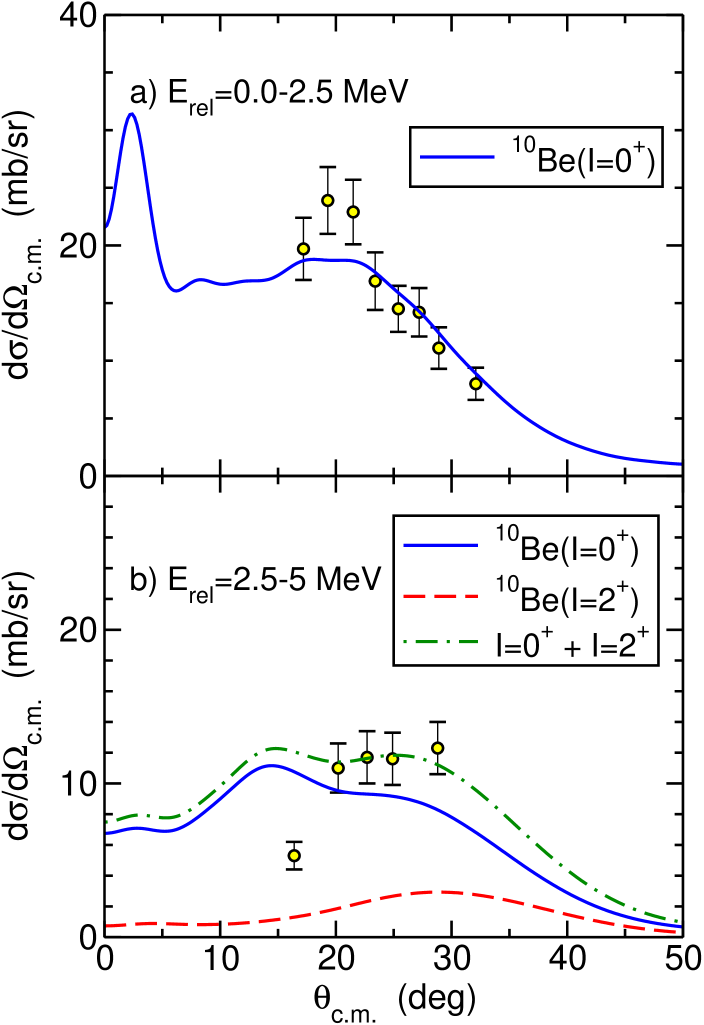
Figure 1: (Color online) Differential breakup cross sections of ¹¹Be on protons at 63.7 MeV/nucleon, with respect to the outgoing ¹¹Be^∗ c.m. scattering angle and the neutron-core relative energy intervals $E_{\mathrm{rel}}=0-2.5$ MeV (top) and $E_{\mathrm{rel}}=2.5-5$ MeV (bottom). The contributions corresponding to the considered outgoing core states are also shown. See text for details.

This is better seen in Fig. 2, where the differential energy cross section is plotted after integration over the angular variables $\Omega_{K}$ in Eq. (V). The solid line is the full XCDCC calculation, considering the core excitation effects in both the structure and the dynamics of the reaction, and includes the two possible final states of the ¹⁰Be nucleus. The ¹⁰Be(2⁺) contribution (red dashed line) only appears for $E_{\mathrm{rel}}>3.4$ MeV, corresponding to the ¹⁰Be($2^{+}$)+$n$ threshold. As already noted, above this energy, the ¹⁰Be fragments can be produced in either the g.s. or the $2^{+}$ excited state. We also show the calculation omitting the DCE mechanism (green dot-dashed curve) and considering only the CA contributions in the structure of the projectile. By comparing with the total distribution, it becomes apparent that the DCE mechanism is very important in this reaction. In particular, the energy spectrum is dominated by two sharp peaks corresponding to the $5/2^{+}_{1}$ and $3/2^{+}_{1}$ resonances with the latter mostly populated by a DCE mechanism Crespo et al. (2011). Despite the relatively small THO basis, the energy profile of these resonances is accurately reproduced and this highlights the advantage of the pseudo-state method over the binning procedure when describing narrow resonances. Finally, besides the resonant contribution, we also note that there is a non-resonant background at low relative energies and above the ¹⁰Be(2⁺)+$n$ threshold.

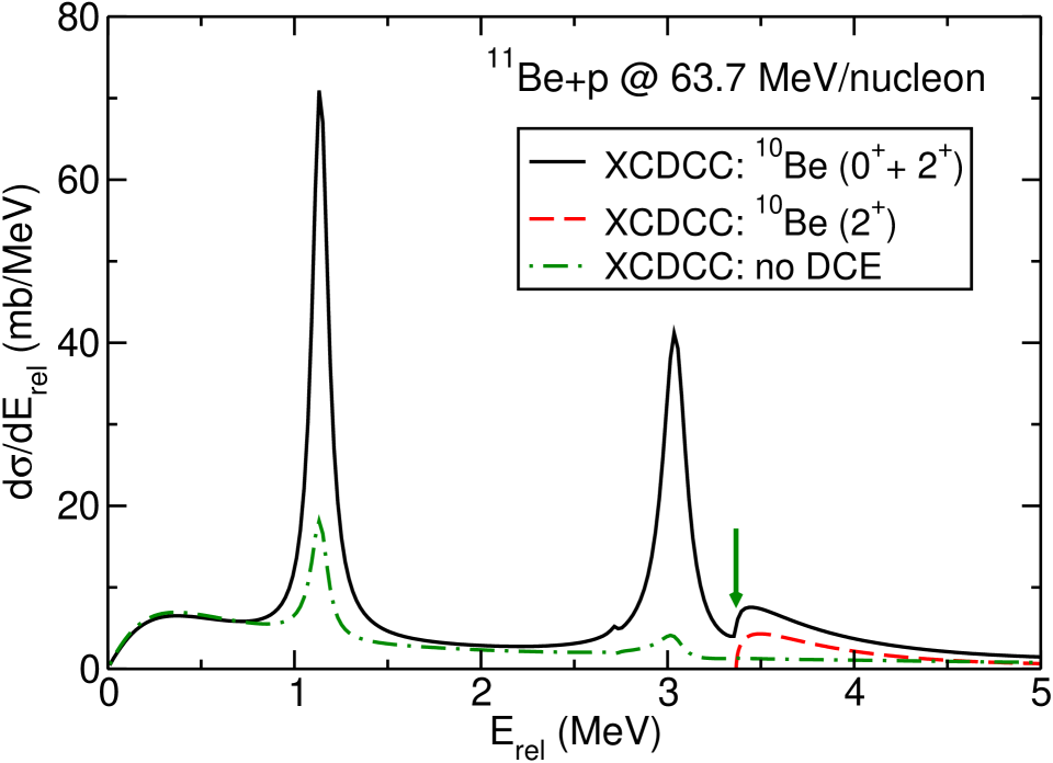
Figure 2: (Color online) Differential energy distribution following the breakup of ¹¹Be on protons at 63.7 MeV/nucleon. Solid and dashed (red) lines correspond to the full ($0^{+}$+$2^{+}$) and the $2^{+}$ contribution of the XCDCC calculation while the dot-dashed line (green) represents the result without dynamic core excitation. The arrow indicates the energy of the ¹⁰Be(2⁺)+$n$ threshold.

Regarding the three-body observables [Eq. (25)], we present in Fig. 3 the energy distributions of the ¹⁰Be fragments from the breakup process at four laboratory angles, plotting separately the $0^{+}$ and $2^{+}$ contributions. We observe from this plot the increasing relative importance of the ¹⁰Be$(2^{+})$ distribution with the angle. This is expected since larger scattering angles of the core implies a stronger interaction with the proton target. It is also apparent that this distribution is shifted to lower energies with respect to the ¹⁰Be(g.s.) due to the higher excitation energy required to produce the ¹⁰Be$(2^{+})$ fragments. The angle-integrated contributions can be seen in Fig. 4, where we note the dominance from the $0^{+}$ component to the overall energy distribution although the $2^{+}$ contribution amounts to 13% of the total cross section at this energy.

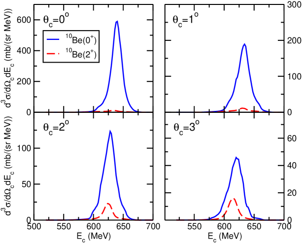
Figure 3: (Color online) Calculated laboratory-frame double differential cross section for the ¹⁰Be fragments emitted in the process ¹¹Be+$p$ at 63.7 MeV/nucleon when four different scattering angles are considered. The blue solid and red dashed lines refer to the contributions from the different core states.

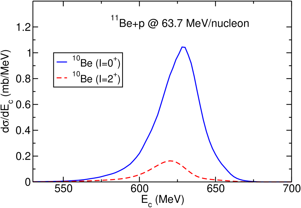
Figure 4: (Color online) Calculated differential energy cross section, as a function of the ¹⁰Be energy in the laboratory frame, for the reaction ¹¹Be+$p$ at 63.7 MeV/nucleon. The solid (blue) and dashed (red) lines describe those calculations when the $I=0$ or $I=2$ state of the core is adopted.

VI.2 ¹¹Be+ ⁶⁴Zn breakup

We consider the ¹¹Be+⁶⁴Zn reaction at 28.7 MeV for which inclusive breakup data have been reported in Ref. Di Pietro et al. (2010) and have been analyzed within the standard CDCC framework in several works Keeley et al. (2010); Di Pietro et al. (2012); Druet and Descouvemont (2012) and also within the XCDCC framework de Diego et al. (2014). The results presented here follow closely those included in this latter reference, but with two main differences: firstly, in that work the ¹⁰Be scattering angle was approximated by the ¹¹Be^∗ angle, assuming two-body kinematics, whereas the appropriate kinematical transformation is applied here; secondly, the XCDCC calculations are performed here in an augmented model space, including higher values of the relative orbital angular momentum between the valence and core particles. In addition, the former analysis is extended by studying the individual contributions of the ¹⁰Be $0^{+}$ and $2^{+}$ states when computing the two- and three-body observables. For the sake of comparison, we also perform standard CDCC calculations similar to those presented in Di Pietro et al. (2012) but using a larger model space, as detailed below.

For the CDCC calculations, ¹¹Be continuum states up to $J=9/2$ (both parities) and $J=11/2^{-}$ were included for maximum $n$-¹⁰Be relative energies and orbital angular momenta $E_{rel}^{\mathrm{max}}=12$ MeV and $\ell_{\mathrm{max}}=5$, respectively. A THO basis with $N=30$ was employed and the involved interactions (i.e., the $n$-¹⁰Be, ¹⁰Be-⁶⁴Zn, and $n$-⁶⁴Zn potentials) were the same as in Ref. Di Pietro et al. (2012) except for that between the neutron and ¹⁰Be. As in Di Pietro et al. (2012), we use for this potential that from Ref. Capel et al. (2004), but we slightly modify the depth for $\ell=2$ in order to reproduce the energy of the $5/2_{1}^{+}$ resonance obtained with the deformed model Be12-b. As for the XCDCC calculations, the following continuum states were considered: for $J\leq 5/2$ (both parities), $\ell_{\mathrm{max}}=3$ and $E_{rel}^{\mathrm{max}}=12$ MeV. For $5/2<J\leq 11/2$, we used $\ell_{\mathrm{max}}=5$ and $E_{rel}^{\mathrm{max}}=9$ MeV. A THO basis with $N=20$ functions was used for all $J^{\pi}$ with the same potentials between the projectile constituents and the target as those used in Ref. de Diego et al. (2014). The coupled equations were solved in this case with the parallelized version of the Fresco coupled-channels code Thompson (1988). The inclusion of high-lying excited states produces numerical instabilities in the solution of the coupled equations. A stabilization procedure similar to that proposed in Baylis and Peel (1982) was used to get stable results.

In Fig. 5 we compare the data from Ref. Di Pietro et al. (2010) with the present calculations. For the XCDCC calculations, the $0^{+}$ and $2^{+}$ contributions are shown separately as solid (blue) or dashed (red) lines, although the latter is found to be negligible in this case. The new CDCC calculation (green dot-dashed curve) appears to be closer to the results with core deformation but both of them clearly underestimate the experimental breakup cross section, in accordance with previous results de Diego et al. (2014). Nevertheless, these former calculations were carried out within a reduced model space and the proper kinematical transformation was not applied. The remaining discrepancy with the data could be due to the contribution of non-elastic breakup events (neutron absorption or target excitation) in the data since the neutrons were not detected in the experiment of Ref. Di Pietro et al. (2010). In this regard, it is worth recalling that the CDCC method provides only the so-called elastic breakup component, so the target is left in the ground state. The inclusion of these non-elastic breakup contributions has been recently the subject of several works Carlson et al. (2016); Lei and Moro (2015); Potel et al. (2015) but the consideration of this effect is beyond the scope of the present work.

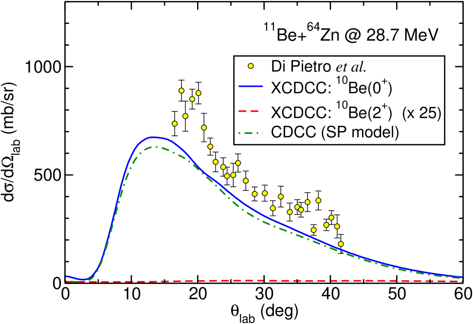
Figure 5: (Color online) Differential cross section, as a function of the laboratory angle, for the ¹⁰Be fragments resulting from the breakup of ¹¹Be on ⁶⁴Zn at $E_{lab}=28.7$ MeV. The solid line (blue) is the calculation when the core ground state, $I=0$, is selected in Eq. (25) after integration over $\Omega_{v}$ and $E_{c}$. The dashed line (red) refers to the $2^{+}$ contribution. A single-particle calculation, omitting the core deformation, is also shown as a dot-dashed curve (green). Experimental data are from Ref. Di Pietro et al. (2010).

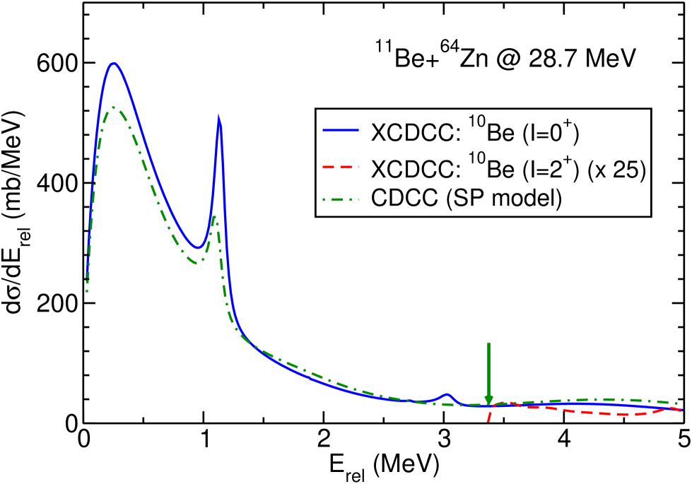
Figure 6: (Color online) Calculated ¹⁰Be differential energy cross section for the reaction ¹¹Be+⁶⁴Zn at 28.7 MeV. The solid (blue) and dashed (red) lines represent the contributions with $I=0$ or $I=2$ as the core states in the two-body distributions (V) after integration over $\Omega_{K}$. The dot-dashed (green) line considers the same calculation without core deformation, assuming a single-particle model for the projectile within the standard CDCC framework. The arrow indicates the energy of the ¹⁰Be(2⁺)+$n$ threshold.

In Fig. 6 we show the breakup cross section as a function of the ¹¹Be excitation energy, with respect to the ¹⁰Be(g.s.)+$n$ threshold. The solid (blue) and dashed (red) lines correspond to the ¹⁰Be(g.s) and ¹⁰Be($2^{+}$) contributions. Most of the cross section is concentrated at low excitation energies, close to the breakup threshold, being negligible for excitation energies above the ¹⁰Be($2^{+}$)+$n$ threshold. Consequently, in this reaction the ¹⁰Be will be mostly produced in its ground state. Moreover, it is remarkable the presence of a prominent peak at energies around the low-lying 5/2⁺ resonance, where the dominant component corresponds to the ¹⁰Be(0⁺) configuration. A second bump, corresponding to the population of the 3/2${}^{+}_{1}$ resonance, can be barely seen. This small contribution reflects the scarce relevance of the DCE mechanism for this medium-mass target as pointed out in Ref. de Diego et al. (2014) but, contrary to the conclusions therein, the core excitation effects in the structure of the ¹¹Be are not so large and the assumption of a single-particle model for the projectile yields a similar breakup cross section (green dot-dashed line). In addition, unlike the case of the proton target, a dominant non-resonant breakup is found at low relative energies.

The different role of DCE for elastic breakup in the cases of the proton and ⁶⁴Zn targets can be ascribed to the dominance of the dipole Coulomb couplings in the latter case, which hinders the effect of the quadrupole couplings associated with the excitation of the ¹⁰Be core. We expect that, for heavier targets, this dominance is enhanced and therefore the effect of the DCE mechanism will be further reduced.

Finally, a small core excitation effect is also apparent in Fig. 7, where we show the breakup energy distributions of the ¹⁰Be emitted fragments within the standard CDCC (only considering the ¹⁰Be(0⁺) state) or XCDCC (including both 0⁺ or 2⁺ states in ¹⁰Be) reaction formalisms at four laboratory angles. The relative importance of the $2^{+}$ state increases with increasing angle but its absolute magnitude is negligible in all cases. It is also observed an overall reduction of the mean energy of the 2⁺ core state, as a consequence of the more negative Q-value. The corresponding angle-integrated energy distribution is shown in Fig. 8. As expected, this distribution is completely dominated by the ¹⁰Be(g.s.) contribution, displaying an asymmetric shape with a maximum around 26 MeV and a large low-energy tail extending down to 15 MeV. For core energies above the peak, the distribution exhibits a pronounced drop as a consequence of the kinematical cutoff from the energy conservation together with the interaction between the phase space factor and the breakup amplitude in the semi-inclusive cross section. Actually, the sharp falloff would be present unless the breakup amplitude is very small around the maximum energy Crespo et al. (2009).

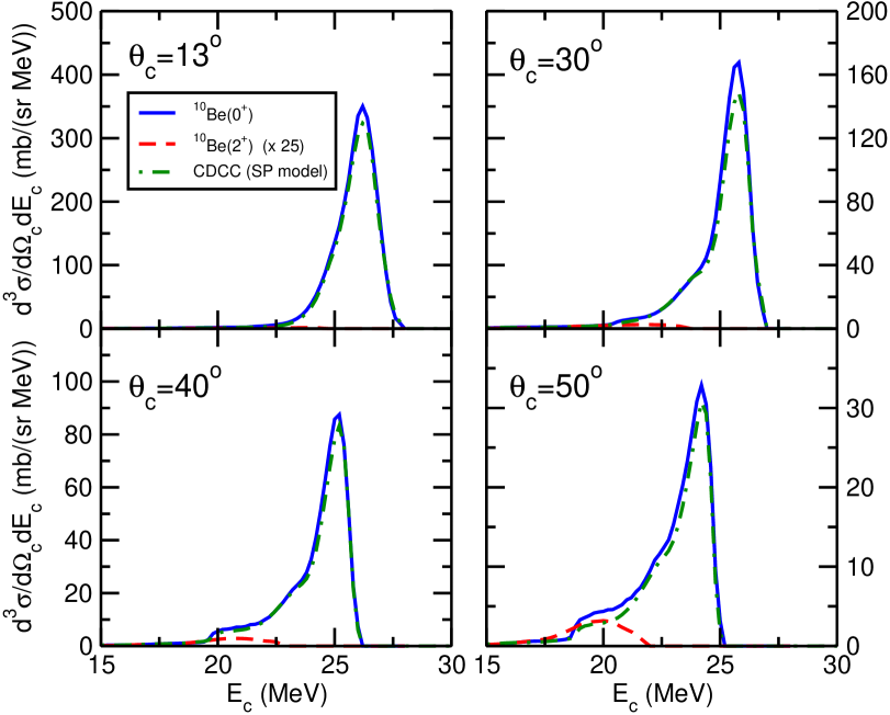
Figure 7: (Color online) Calculated laboratory frame ¹⁰Be cross section energy distributions for the process ¹¹Be+⁶⁴Zn at 28.7 MeV with different laboratory angles in Eq. (25). Under the XCDCC framework we study both the $0^{+}$ (blue solid) or $2^{+}$ (red dashed) contributions while the standard CDCC method provides the distributions without core deformation (green dot-dashed).

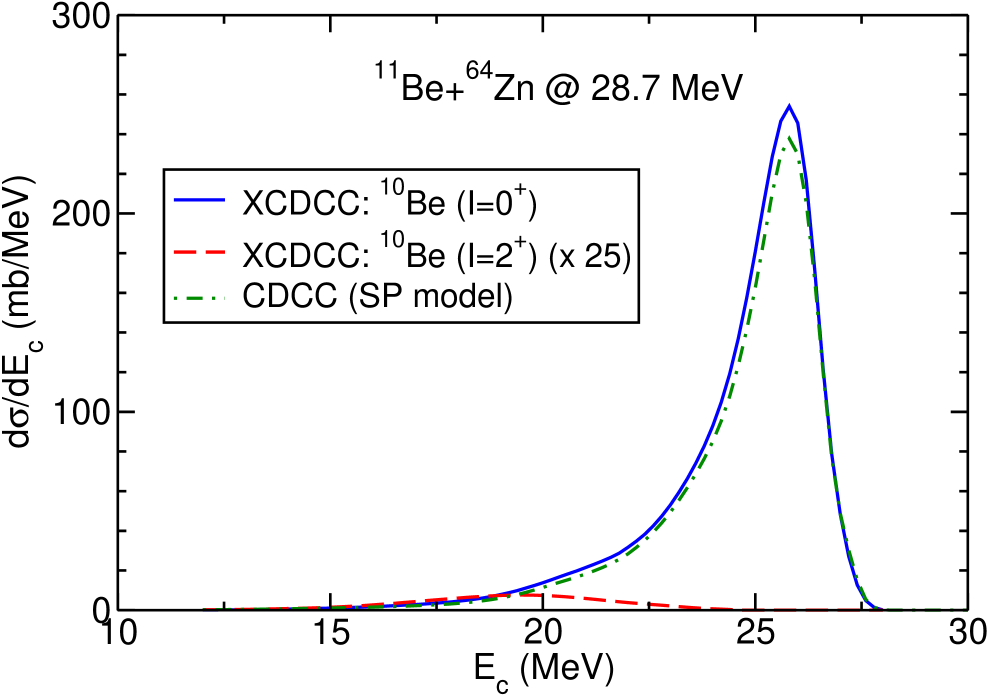
Figure 8: (Color online) Calculated laboratory frame ¹⁰Be differential energy cross section for the breakup reaction ¹¹Be+⁶⁴Zn at 28.7 MeV. The blue solid and red dashed lines account for the components obtained with the different core states in the XCDCC calculation. The distribution computed with the standard CDCC method (no deformation) is also shown (green dot-dashed).

VII Summary and conclusions

In this paper we have presented a formalism for the calculation of two- and three-body breakup observables from XCDCC calculations. The method has been applied to the case of the scattering of a two-body projectile consisting on a core and a valence particle, and taking explicitly into account core excitations. The method is based on a convolution of the discrete XCDCC scattering amplitudes with the exact core+valence scattering states. The formalism is a natural extension of that presented in Ref. Tostevin et al. (2001) for the standard CDCC method, the main difference being the multi-channel character of the projectile states in the present case. The convoluted transition amplitudes are then multiplied by the corresponding phase-space factor to produce the desired (two- or three-body) differential cross sections. The formalism provides the separate cross section for specific states of the core nucleus, thus permitting a more direct connection with experimental observables.

The method has been applied to the scattering of ¹¹Be on protons and ⁶⁴Zn. The ¹¹Be nucleus is described in a simple particle-rotor model, in which the ¹⁰Be core is assumed to have a permanent axial deformation Nunes et al. (1996). The core-target interaction is obtained by deforming a central phenomenological potential. Within the developed approach the angular and energy distributions of the ¹⁰Be fragments (with an intrinsic spin, $I$) following the breakup of ¹¹Be have been calculated and compared with experimental data, when available.

In the ¹¹Be+$p$ reaction, we find that a significant part of the breakup cross section corresponds to the ¹⁰Be excited state. Moreover, we have confirmed the importance of the DCE mechanism, arising from the non-central part of the core-target interaction, for the excitation of the low-lying $5/2^{+}$ and $3/2^{+}$ resonances Moro and Crespo (2012).

We have also studied the ¹¹Be+⁶⁴Zn reaction at 28.7 MeV, extending the previous analysis performed in Ref. de Diego et al. (2014). Although in that reference a sizable difference was observed between the calculations with and without deformation, the present calculations suggest that this difference is largely reduced if a sufficiently large model space is employed for the XCDCC calculation. In view of these new results, we may conclude that, unlike the proton target case, the effect of core excitation is very small in this reaction as far as the breakup cross sections concern. As a consequence, the ¹⁰Be(2⁺) yield is found to be negligibly small. We may anticipate that this conclusion will also hold for other medium-mass or heavy systems. The qualitative difference with respect to the proton case stems from the larger importance of Coulomb couplings in the ⁶⁴Zn case.

Although all the calculations presented in this work have been performed for the ¹¹Be nucleus, we believe that the results are extrapolable to other weakly-bound nuclei and, consequently, the effects discussed here should be taken in consideration for an accurate description and interpretation of the data. Finally, we notice that the semi-inclusive differential cross sections presented in this paper can be used to produce transverse and longitudinal momentum distributions, which have been used to obtain spectroscopic information using both light and proton targets.

Appendix A Calculation of multi-channel scattering states

Here we derive the coefficients $C_{\ell,j,J,M}$, that relate the scattering states with the solution of the Schrödinder equation for good values of $J,M$ according to the expansion

$$\phi_{{\mathbf{k}}_{I};I\mu;s\sigma}^{(+)}({\mathbf{r}},\xi_{v},\xi_{c})=\sum_{\ell,j,J,M}C_{\ell,j,J,M}\Psi^{(+)}_{\alpha,J,M}(k_{I},{\mathbf{r}},\xi_{v},\xi_{c}).$$ (28)

The expansion coefficients are determined by replacing the functions $\Psi^{(+)}_{\alpha,J,M}(k_{I},{\mathbf{r}},\xi_{v},\xi_{c})$ by their asymptotic behaviour, Eq. (15),

$$\phi_{{\mathbf{k}}_{I};I\mu;s\sigma}^{(+)}({\mathbf{r}},\xi_{v},\xi_{c}) \rightarrow\sum_{\ell,j,J,M}e^{i\sigma_{\ell}}C_{\ell,j,J,M}\sum_{\alpha^{\prime}}\left[\frac{F_{\ell}(k_{I}r)}{r}\delta_{\ell,\ell^{\prime}}\right.$$

$$+\left.T^{J}_{\alpha,\alpha^{\prime}}\frac{H^{(+)}_{\ell^{\prime}}(k_{I}r)}{r}\right]\Phi_{\alpha^{\prime},J,M}(\hat{r},\xi_{v},\xi_{c})$$

where, in the r.h.s. of the equation, we have separated for convenience the part containing the regular Coulomb function.

To compare this with the asymptotic behaviour we need the partial-wave decomposition of the plane wave:

$$e^{i{\mathbf{k}}_{I}\cdot{\mathbf{r}}}=\frac{4\pi}{k_{I}r}\sum_{\ell,m}i^{\ell}(k_{I}r)j_{\ell}(k_{I}r)Y^{*}_{\ell m}(\hat{k_{I}})Y_{\ell m}(\hat{r}).$$ (30)

More generally, in presence of Coulomb, the expansion above becomes:

$$\chi_{C}({{\mathbf{k}}_{I},{\mathbf{r}}})=\frac{4\pi}{k_{I}r}\sum_{\ell,m}i^{\ell}e^{i\sigma_{\ell}}F_{\ell}(k_{I}r)Y^{*}_{\ell m}(\hat{k_{I}})Y_{\ell m}(\hat{r}).$$ (31)

Using this result, the plane wave reads:

$$\chi_{C}({{\mathbf{k}}_{I},{\mathbf{r}}})\varphi^{(v)}_{s\sigma}(\xi_{v})\varphi^{(c)}_{I\mu}(\xi_{c})=$$

$$\frac{4\pi}{k_{I}r}\sum_{\ell,m}i^{\ell}e^{i\sigma_{\ell}}F_{\ell}(k_{I}r)Y^{*}_{\ell m}(\hat{k_{I}})Y_{\ell m}(\hat{r})\varphi^{(v)}_{s\sigma}(\xi_{v})\varphi^{(c)}_{I\mu}(\xi_{c}).$$

In oder to express this state in terms of the basis (8), we use the following expansions:

$$Y_{\ell m}(\hat{r})\varphi^{(v)}_{s\sigma}(\xi_{v})=\sum_{j,m_{j}}\langle\ell ms\sigma|jm_{j}\rangle{\cal Y}_{(\ell s)jm_{j}}(\hat{r},\xi_{v})$$ (33)

$${\cal Y}_{(\ell s)jm_{j}}(\hat{r},\xi_{v})\varphi^{(c)}_{I\mu}(\xi_{c})=\sum_{JM}\langle jm_{j}I\mu|JM\rangle\Phi_{\alpha,J,M}(\hat{r},\xi_{v},\xi_{c}).$$ (34)

So, collecting results,

$$\chi_{C}({{\mathbf{k}}_{I},{\mathbf{r}}})\varphi^{(v)}_{s\sigma}(\xi_{v})\varphi^{(c)}_{I\mu}(\xi_{c}) =\frac{4\pi}{k_{I}r}\sum_{\ell,m}Y^{*}_{\ell m}(\hat{k_{I}})i^{\ell}e^{i\sigma_{\ell}}F_{\ell}(k_{I}r)\sum_{j,m_{j}}\sum_{J,M}\langle\ell ms\sigma|jm_{j}\rangle\langle jm_{j}I\mu|JM\rangle\Phi_{\alpha,J,M}(\hat{r},\xi_{v},\xi_{c}).$$ (35)

The above expression gives the plane-wave part of Eq. (LABEL:phi_asym_coefs), so we get for the $C$ coefficients:

$$C_{\ell,j,J,M}=\frac{4\pi}{k_{I}}\sum_{m,m_{j}}i^{\ell}Y^{*}_{\ell m}(\hat{k_{I}})\langle\ell ms\sigma|jm_{j}\rangle\langle jm_{j}I\mu|JM\rangle.$$ (36)

Therefore, the scattering states $\phi_{{\mathbf{k}}_{I};I\mu;s\sigma}^{(+)}({\mathbf{r}},\xi_{v},\xi_{c})$ are expressed as follows:

$$\phi_{{\mathbf{k}}_{I};I\mu;s\sigma}^{(+)}({\mathbf{r}},\xi_{v},\xi_{c})$$ (37)

$$= \frac{4\pi}{k_{I}r}\sum_{\ell,j,J,M}i^{\ell}Y^{*}_{\ell m}(\hat{k_{I}})\langle\ell ms\sigma|jm_{j}\rangle\langle jm_{j}I\mu|JM\rangle$$

$$\times\sum_{\alpha^{\prime}}f^{J}_{\alpha:\alpha^{\prime}}(k_{I},r)\Phi_{\alpha^{\prime},J,M}(\hat{r},\xi_{v},\xi_{c}),$$

where $m_{j}=M-\mu$, and $m=m_{j}-\sigma$.

The scattering states appearing in the T-matrix amplitude, Eq. (18), are $(\phi_{{\mathbf{k}}_{I};I\mu;s\sigma}^{(-)}({\mathbf{r}},\xi_{v},\xi_{c}))^{*}$, which can be derived from $\phi_{{\mathbf{k}}_{I};I\mu;s\sigma}^{(+)}({\mathbf{r}},\xi_{v},\xi_{c})$ by application of the time-reversal operator, resulting Howell (2008),

$$(\phi_{{\mathbf{k}}_{I};I\mu;s\sigma}^{(-)}({\mathbf{r}},\xi_{v},\xi_{c}))^{*}=\frac{4\pi}{k_{I}r}\sum_{\begin{subarray}{c}\ell,j,m,m_{j}\\ J,M\end{subarray}}i^{\ell}Y_{\ell m}(\hat{k_{I}})\langle\ell ms\sigma|jm_{j}\rangle\langle jm_{j}I\mu|JM\rangle\sum_{\alpha^{\prime}}(-1)^{\ell^{\prime}+I+I^{\prime}}f^{J}_{\alpha:\alpha^{\prime}}(k_{I},r)\Phi^{*}_{\alpha^{\prime},J,M}(\hat{r},\xi_{v},\xi_{c}).$$ (38)

Appendix B Overlap functions

Starting from the states (38), and writing the THO eigenstates for a given angular momentum and projection $J^{\prime},M^{\prime}$ as:

$$\Psi^{(N)}_{i,J^{\prime},M^{\prime}}({\mathbf{r}},\xi_{v},\xi_{c})=\sum_{\alpha^{\prime\prime}}\frac{g_{i,\alpha^{\prime\prime}}^{J^{\prime}}(r)}{r}\Phi_{\alpha^{\prime\prime},J^{\prime},M^{\prime}}(\hat{r},\xi_{v},\xi_{c}),$$ (39)

the overlap between them yields

$$\langle\phi_{\bm{k}_{I};I\mu;s\sigma}^{(-)}|\Psi^{(N)}_{i,J^{\prime},M^{\prime}}\rangle =\frac{4\pi}{k_{I}}\sum_{\ell,m,j}(-i)^{\ell}Y_{\ell m}(\hat{k_{I}})\langle\ell ms\sigma|jm_{j}\rangle$$

$$\times\langle jm_{j}I\mu|J^{\prime}M^{\prime}\rangle{\cal G}_{\alpha}^{i,J^{\prime}}(k_{I}),$$ (40)

which, in addition to geometric coefficients, contain the function ${\cal G}_{\alpha}^{i,J^{\prime}}(k_{I})=\sum_{\alpha^{\prime}}(-1)^{\ell+\ell^{\prime}+I+I^{\prime}}{\cal O}_{\alpha,\alpha^{\prime}}^{i,J^{\prime}}(k_{I})$, with the ${\cal O}_{\alpha,\alpha^{\prime}}^{J}(k_{I})$ representing the overlaps between the radial functions:

$${\cal O}_{\alpha,\alpha^{\prime}}^{i,J}(k_{I})=\int f^{J}_{\alpha:\alpha^{\prime}}(k_{I},r)g_{i,\alpha^{\prime}}^{J}(r)dr.$$ (41)

We also note that the total parity of the pseudo-states, $\Psi^{(N)}_{i,J^{\prime},M^{\prime}}({\mathbf{r}},\xi_{v},\xi_{c})$, is given by the factor $(-1)^{\ell+I}$ and, consequently, the phase appearing in the function ${\cal G}_{\alpha}^{i,J^{\prime}}(k_{I})$ is equal to one.

References

- Nakamura and Kondo (2012) T. Nakamura and Y. Kondo, Clusters in Nuclei, Vol.2, Lecture Notes in Physics, vol. 848 (Springer-Verlag Berlin Heidelberg, 2012), C. Beck ed.
- Rawitscher (1974) G. H. Rawitscher, Phys. Rev. C 9, 2210 (1974).
- Austern et al. (1987) N. Austern, Y. Iseri, M. Kamimura, M. Kawai, G. Rawitscher, and M. Yahiro, Phys. Rep. 154, 125 (1987).
- Banerjee and Shyam (2000) P. Banerjee and R. Shyam, Phys. Rev. C 61, 047301 (2000).
- Tostevin et al. (1998) J. A. Tostevin, S. Rugmai, and R. C. Johnson, Phys. Rev. C 57, 3225 (1998).
- Faddeev (1960) L. D. Faddeev, Zh. Eksp. Theor. Fiz. 39, 1459 (1960), [Sov. Phys. JETP 12, 1014 (1961)].
- Alt et al. (1967) E. O. Alt, P. Grassberger, and W. Sandhas, Nucl. Phys. B 2, 167 (1967).
- Typel and Baur (1994) S. Typel and G. Baur, Phys. Rev. C 50, 2104 (1994).
- Esbensen and Bertsch (1996) H. Esbensen and G. F. Bertsch, Nucl. Phys. A 600, 37 (1996).
- Kido et al. (1994) T. Kido, K. Yabana, and Y. Suzuki, Phys. Rev. C 50, R1276 (1994).
- Typel and Baur (2001) S. Typel and G. Baur, Phys. Rev. C 64, 024601 (2001).
- Capel et al. (2004) P. Capel, G. Goldstein, and D. Baye, Phys. Rev. C 70, 064605 (2004).
- García-Camacho et al. (2006) A. García-Camacho, A. Bonaccorso, and D. M. Brink, Nucl. Phys. A 776, 118 (2006).
- Lay et al. (2012) J. A. Lay, A. M. Moro, J. M. Arias, and J. Gómez-Camacho, Phys. Rev. C 85, 054618 (2012).
- Crespo et al. (2011) R. Crespo, A. Deltuva, and A. M. Moro, Phys. Rev. C 83, 044622 (2011).
- Moro and Crespo (2012) A. M. Moro and R. Crespo, Phys. Rev. C 85, 054613 (2012).
- Moro and Lay (2012) A. M. Moro and J. A. Lay, Phys. Rev. Lett. 109, 232502 (2012).
- Moro et al. (2012) A. M. Moro, R. de Diego, J. A. Lay, R. Crespo, R. C. Johnson, J. M. Arias, and J. Gómez-Camacho, in AIP Conference Proceedings-American Institute of Physics (2012), vol. 1491, p. 335.
- de Diego et al. (2014) R. de Diego, J. M. Arias, and A. M. Moro, Phys. Rev. C 89, 064609 (2014).
- Summers et al. (2006) N. C. Summers, F. M. Nunes, and I. J. Thompson, Phys. Rev. C 74, 014606 (2006).
- Lay et al. (2016) J. A. Lay, R. de Diego, R. Crespo, A. M. Moro, J. M. Arias, and R. C. Johnson, Phys. Rev. C 94, 021602(R) (2016).
- Deltuva (2015) A. Deltuva, Phys. Rev. C 91, 024607 (2015).
- Deltuva et al. (2016) A. Deltuva, A. Ross, E. Norvaišas, and F. M. Nunes, Phys. Rev. C 94, 044613 (2016).
- Aarts et al. (1984) E. Aarts, R. Malfliet, R. De Meijer, and S. Van Der Werf, Nuclear Physics A 425, 23 (1984).
- Tostevin et al. (2001) J. A. Tostevin, F. M. Nunes, and I. J. Thompson, Phys. Rev. C 63, 024617 (2001).
- Di Pietro et al. (2010) A. Di Pietro, G. Randisi, V. Scuderi, L. Acosta, F. Amorini, M. J. G. Borge, P. Figuera, M. Fisichella, L. M. Fraile, J. Gomez-Camacho, et al., Phys. Rev. Lett. 105, 022701 (2010).
- Matsumoto et al. (2003) T. Matsumoto, T. Kamizato, K. Ogata, Y. Iseri, E. Hiyama, M. Kamimura, and M. Yahiro, Phys. Rev. C 68, 064607 (2003).
- Bohr and Mottelson (1969) A. Bohr and B. Mottelson, Nuclear Structure (1969), New York, W. A. Benjamin ed.
- Tamura (1965) T. Tamura, Rev. Mod. Phys. 37, 679 (1965).
- Fuchs (1982) H. Fuchs, Nucl. Instrum. Methods Phys. Res. 200, 361 (1982).
- Fortier et al. (1999) S. Fortier et al., Phys. Lett. B 461, 22 (1999).
- Winfield et al. (2001) J. S. Winfield et al., Nucl. Phys. A 683, 48 (2001).
- Cappuzzello et al. (2001) F. Cappuzzello, A. Cunsolo, S. Fortier, A. Foti, M. Khaled, H. Laurent, H. Lenske, J. M. Maison, A. L. Melita, C. Nociforo, et al., Phys. Lett. B 516, 21 (2001).
- Chen et al. (2016) J. Chen, J. Lou, Y. Ye, Z. Li, Y. Ge, Q. Li, J. Li, W. Jiang, Y. Sun, H. Zang, et al., Physical Review C 93, 034623 (2016).
- Nunes et al. (1996) F. M. Nunes, J. A. Christley, I. J. Thompson, R. C. Johnson, and V. D. Efros, Nucl. Phys. A 609, 43 (1996).
- Kelley et al. (2012) J. H. Kelley et al., Nucl. Phys. A 880, 88 (2012), ISSN 0375-9474.
- Jeukenne et al. (1977) J. P. Jeukenne, A. Lejeune, and C. Mahaux, Phys. Rev. C 16, 80 (1977).
- Takashina and Kanada-Enyo (2008) M. Takashina and Y. Kanada-Enyo, Phys.Rev. C 77, 014604 (2008).
- Cortina-Gil et al. (1997) M. D. Cortina-Gil, P. Roussel-Chomaz, N. Alamanos, J. Barrette, W. Mittig, F. S. Dietrich, F. Auger, Y. Blumenfeld, J. M. Casandjian, M. Chartier, et al., Phys. Lett. B 401, 9 (1997).
- Shrivastava et al. (2004) A. Shrivastava et al., Phys. Lett. B 596, 54 (2004).
- Keeley et al. (2010) N. Keeley, N. Alamanos, K. W. Kemper, and K. Rusek, Phys. Rev. C 82, 034606 (2010).
- Di Pietro et al. (2012) A. Di Pietro, V. Scuderi, A. M. Moro, L. Acosta, F. Amorini, M. J. G. Borge, P. Figuera, M. Fisichella, L. M. Fraile, J. Gomez-Camacho, et al., Phys. Rev. C 85, 054607 (2012).
- Druet and Descouvemont (2012) T. Druet and P. Descouvemont, Eur. Phys. J. A 48, 147 (2012).
- Thompson (1988) I. J. Thompson, Comp. Phys. Rep. 7, 167 (1988).
- Baylis and Peel (1982) W. E. Baylis and S. J. Peel, Comp. Phys. Comm. 25, 7 (1982).
- Carlson et al. (2016) B. V. Carlson, R. Capote, and M. Sin, Few-Body Systems 57, 307 (2016).
- Lei and Moro (2015) J. Lei and A. M. Moro, Phys. Rev. C 92, 044616 (2015).
- Potel et al. (2015) G. Potel, F. M. Nunes, and I. J. Thompson, Phys. Rev. C 92, 034611 (2015).
- Crespo et al. (2009) R. Crespo, A. Deltuva, M. Rodríguez-Gallardo, E. Cravo, and A. C. Fonseca, Phys. Rev. C 79, 014609 (2009).
- Howell (2008) D. J. Howell, Ph.D. thesis, University of Surrey (2008).