M. Ablikim1, M. N. Achasov9,e, S. Ahmed14, X. C. Ai1, O. Albayrak5, M. Albrecht4, D. J. Ambrose44, A. Amoroso49A,49C, F. F. An1, Q. An46,a, J. Z. Bai1, R. Baldini Ferroli20A, Y. Ban31, D. W. Bennett19, J. V. Bennett5, N. B. Berger22, M. Bertani20A, D. Bettoni21A, J. M. Bian43, F. Bianchi49A,49C, E. Boger23,c, I. Boyko23, R. A. Briere5, H. Cai51, X. Cai1,a, O. Cakir40A, A. Calcaterra20A, G. F. Cao1, S. A. Cetin40B, J. F. Chang1,a, G. Chelkov23,c,d, G. Chen1, H. S. Chen1, H. Y. Chen2, J. C. Chen1, M. L. Chen1,a, S. Chen41, S. J. Chen29, X. Chen1,a, X. R. Chen26, Y. B. Chen1,a, H. P. Cheng17, X. K. Chu31, G. Cibinetto21A, H. L. Dai1,a, J. P. Dai34, A. Dbeyssi14, D. Dedovich23, Z. Y. Deng1, A. Denig22, I. Denysenko23, M. Destefanis49A,49C, F. De Mori49A,49C, Y. Ding27, C. Dong30, J. Dong1,a, L. Y. Dong1, M. Y. Dong1,a, Z. L. Dou29, S. X. Du53, P. F. Duan1, J. Z. Fan39, J. Fang1,a, S. S. Fang1, X. Fang46,a, Y. Fang1, R. Farinelli21A,21B, L. Fava49B,49C, O. Fedorov23, F. Feldbauer22, G. Felici20A, C. Q. Feng46,a, E. Fioravanti21A, M. Fritsch14,22, C. D. Fu1, Q. Gao1, X. L. Gao46,a, X. Y. Gao2, Y. Gao39, Z. Gao46,a, I. Garzia21A, K. Goetzen10, L. Gong30, W. X. Gong1,a, W. Gradl22, M. Greco49A,49C, M. H. Gu1,a, Y. T. Gu12, Y. H. Guan1, A. Q. Guo1, L. B. Guo28, R. P. Guo1, Y. Guo1, Y. P. Guo22, Z. Haddadi25, A. Hafner22, S. Han51, X. Q. Hao15, F. A. Harris42, K. L. He1, F. H. Heinsius4, T. Held4, Y. K. Heng1,a, T. Holtmann4, Z. L. Hou1, C. Hu28, H. M. Hu1, J. F. Hu49A,49C, T. Hu1,a, Y. Hu1, G. S. Huang46,a, J. S. Huang15, X. T. Huang33, X. Z. Huang29, Y. Huang29, Z. L. Huang27, T. Hussain48, Q. Ji1, Q. P. Ji30, X. B. Ji1, X. L. Ji1,a, L. W. Jiang51, X. S. Jiang1,a, X. Y. Jiang30, J. B. Jiao33, Z. Jiao17, D. P. Jin1,a, S. Jin1, T. Johansson50, A. Julin43, N. Kalantar-Nayestanaki25, X. L. Kang1, X. S. Kang30, M. Kavatsyuk25, B. C. Ke5, P. Kiese22, R. Kliemt14, B. Kloss22, O. B. Kolcu40B,h, B. Kopf4, M. Kornicer42, A. Kupsc50, W. Kühn24, J. S. Lange24, M. Lara19, P. Larin14, H. Leithoff22, C. Leng49C, C. Li50, Cheng Li46,a, D. M. Li53, F. Li1,a, F. Y. Li31, G. Li1, H. B. Li1, H. J. Li1, J. C. Li1, Jin Li32, K. Li13, K. Li33, Lei Li3, P. R. Li41, Q. Y. Li33, T. Li33, W. D. Li1, W. G. Li1, X. L. Li33, X. M. Li12, X. N. Li1,a, X. Q. Li30, Y. B. Li2, Z. B. Li38, H. Liang46,a, J. J. Liang12, Y. F. Liang36, Y. T. Liang24, G. R. Liao11, D. X. Lin14, B. Liu34, B. J. Liu1, C. X. Liu1, D. Liu46,a, F. H. Liu35, Fang Liu1, Feng Liu6, H. B. Liu12, H. H. Liu1, H. H. Liu16, H. M. Liu1, J. Liu1, J. B. Liu46,a, J. P. Liu51, J. Y. Liu1, K. Liu39, K. Y. Liu27, L. D. Liu31, P. L. Liu1,a, Q. Liu41, S. B. Liu46,a, X. Liu26, Y. B. Liu30, Y. Y. Liu30, Z. A. Liu1,a, Zhiqing Liu22, H. Loehner25, X. C. Lou1,a,g, H. J. Lu17, J. G. Lu1,a, Y. Lu1, Y. P. Lu1,a, C. L. Luo28, M. X. Luo52, T. Luo42, X. L. Luo1,a, X. R. Lyu41, F. C. Ma27, H. L. Ma1, L. L. Ma33, M. M. Ma1, Q. M. Ma1, T. Ma1, X. N. Ma30, X. Y. Ma1,a, Y. M. Ma33, F. E. Maas14, M. Maggiora49A,49C, Q. A. Malik48, Y. J. Mao31, Z. P. Mao1, S. Marcello49A,49C, J. G. Messchendorp25, G. Mezzadri21B, J. Min1,a, R. E. Mitchell19, X. H. Mo1,a, Y. J. Mo6, C. Morales Morales14, N. Yu. Muchnoi9,e, H. Muramatsu43, P. Musiol4, Y. Nefedov23, F. Nerling14, I. B. Nikolaev9,e, Z. Ning1,a, S. Nisar8, S. L. Niu1,a, X. Y. Niu1, S. L. Olsen32, Q. Ouyang1,a, S. Pacetti20B, Y. Pan46,a, P. Patteri20A, M. Pelizaeus4, H. P. Peng46,a, K. Peters10, J. Pettersson50, J. L. Ping28, R. G. Ping1, R. Poling43, V. Prasad1, H. R. Qi2, M. Qi29, S. Qian1,a, C. F. Qiao41, L. Q. Qin33, N. Qin51, X. S. Qin1, Z. H. Qin1,a, J. F. Qiu1, K. H. Rashid48, C. F. Redmer22, M. Ripka22, G. Rong1, Ch. Rosner14, X. D. Ruan12, A. Sarantsev23,f, M. Savrié21B, C. Schnier4, K. Schoenning50, S. Schumann22, W. Shan31, M. Shao46,a, C. P. Shen2, P. X. Shen30, X. Y. Shen1, H. Y. Sheng1, M. Shi1, W. M. Song1, X. Y. Song1, S. Sosio49A,49C, S. Spataro49A,49C, G. X. Sun1, J. F. Sun15, S. S. Sun1, X. H. Sun1, Y. J. Sun46,a, Y. Z. Sun1, Z. J. Sun1,a, Z. T. Sun19, C. J. Tang36, X. Tang1, I. Tapan40C, E. H. Thorndike44, M. Tiemens25, I. Uman40D, G. S. Varner42, B. Wang30, B. L. Wang41, D. Wang31, D. Y. Wang31, K. Wang1,a, L. L. Wang1, L. S. Wang1, M. Wang33, P. Wang1, P. L. Wang1, S. G. Wang31, W. Wang1,a, W. P. Wang46,a, X. F. Wang39, Y. Wang37, Y. D. Wang14, Y. F. Wang1,a, Y. Q. Wang22, Z. Wang1,a, Z. G. Wang1,a, Z. H. Wang46,a, Z. Y. Wang1, Z. Y. Wang1, T. Weber22, D. H. Wei11, J. B. Wei31, P. Weidenkaff22, S. P. Wen1, U. Wiedner4, M. Wolke50, L. H. Wu1, L. J. Wu1, Z. Wu1,a, L. Xia46,a, L. G. Xia39, Y. Xia18, D. Xiao1, H. Xiao47, Z. J. Xiao28, Y. G. Xie1,a, Q. L. Xiu1,a, G. F. Xu1, J. J. Xu1, L. Xu1, Q. J. Xu13, Q. N. Xu41, X. P. Xu37, L. Yan49A,49C, W. B. Yan46,a, W. C. Yan46,a, Y. H. Yan18, H. J. Yang34, H. X. Yang1, L. Yang51, Y. X. Yang11, M. Ye1,a, M. H. Ye7, J. H. Yin1, B. X. Yu1,a, C. X. Yu30, J. S. Yu26, C. Z. Yuan1, W. L. Yuan29, Y. Yuan1, A. Yuncu40B,b, A. A. Zafar48, A. Zallo20A, Y. Zeng18, Z. Zeng46,a, B. X. Zhang1, B. Y. Zhang1,a, C. Zhang29, C. C. Zhang1, D. H. Zhang1, H. H. Zhang38, H. Y. Zhang1,a, J. Zhang1, J. J. Zhang1, J. L. Zhang1, J. Q. Zhang1, J. W. Zhang1,a, J. Y. Zhang1, J. Z. Zhang1, K. Zhang1, L. Zhang1, S. Q. Zhang30, X. Y. Zhang33, Y. Zhang1, Y. H. Zhang1,a, Y. N. Zhang41, Y. T. Zhang46,a, Yu Zhang41, Z. H. Zhang6, Z. P. Zhang46, Z. Y. Zhang51, G. Zhao1, J. W. Zhao1,a, J. Y. Zhao1, J. Z. Zhao1,a, Lei Zhao46,a, Ling Zhao1, M. G. Zhao30, Q. Zhao1, Q. W. Zhao1, S. J. Zhao53, T. C. Zhao1, Y. B. Zhao1,a, Z. G. Zhao46,a, A. Zhemchugov23,c, B. Zheng47, J. P. Zheng1,a, W. J. Zheng33, Y. H. Zheng41, B. Zhong28, L. Zhou1,a, X. Zhou51, X. K. Zhou46,a, X. R. Zhou46,a, X. Y. Zhou1, K. Zhu1, K. J. Zhu1,a, S. Zhu1, S. H. Zhu45, X. L. Zhu39, Y. C. Zhu46,a, Y. S. Zhu1, Z. A. Zhu1, J. Zhuang1,a, L. Zotti49A,49C, B. S. Zou1, J. H. Zou1(BESIII Collaboration)1 Institute of High Energy Physics, Beijing 100049, People’s Republic of China
2 Beihang University, Beijing 100191, People’s Republic of China
3 Beijing Institute of Petrochemical Technology, Beijing 102617, People’s Republic of China
4 Bochum Ruhr-University, D-44780 Bochum, Germany
5 Carnegie Mellon University, Pittsburgh, Pennsylvania 15213, USA
6 Central China Normal University, Wuhan 430079, People’s Republic of China
7 China Center of Advanced Science and Technology, Beijing 100190, People’s Republic of China
8 COMSATS Institute of Information Technology, Lahore, Defence Road, Off Raiwind Road, 54000 Lahore, Pakistan
9 G.I. Budker Institute of Nuclear Physics SB RAS (BINP), Novosibirsk 630090, Russia
10 GSI Helmholtzcentre for Heavy Ion Research GmbH, D-64291 Darmstadt, Germany
11 Guangxi Normal University, Guilin 541004, People’s Republic of China
12 GuangXi University, Nanning 530004, People’s Republic of China
13 Hangzhou Normal University, Hangzhou 310036, People’s Republic of China
14 Helmholtz Institute Mainz, Johann-Joachim-Becher-Weg 45, D-55099 Mainz, Germany
15 Henan Normal University, Xinxiang 453007, People’s Republic of China
16 Henan University of Science and Technology, Luoyang 471003, People’s Republic of China
17 Huangshan College, Huangshan 245000, People’s Republic of China
18 Hunan University, Changsha 410082, People’s Republic of China
19 Indiana University, Bloomington, Indiana 47405, USA
20 (A)INFN Laboratori Nazionali di Frascati, I-00044, Frascati, Italy; (B)INFN and University of Perugia, I-06100, Perugia, Italy
21 (A)INFN Sezione di Ferrara, I-44122, Ferrara, Italy; (B)University of Ferrara, I-44122, Ferrara, Italy
22 Johannes Gutenberg University of Mainz, Johann-Joachim-Becher-Weg 45, D-55099 Mainz, Germany
23 Joint Institute for Nuclear Research, 141980 Dubna, Moscow region, Russia
24 Justus-Liebig-Universitaet Giessen, II. Physikalisches Institut, Heinrich-Buff-Ring 16, D-35392 Giessen, Germany
25 KVI-CART, University of Groningen, NL-9747 AA Groningen, The Netherlands
26 Lanzhou University, Lanzhou 730000, People’s Republic of China
27 Liaoning University, Shenyang 110036, People’s Republic of China
28 Nanjing Normal University, Nanjing 210023, People’s Republic of China
29 Nanjing University, Nanjing 210093, People’s Republic of China
30 Nankai University, Tianjin 300071, People’s Republic of China
31 Peking University, Beijing 100871, People’s Republic of China
32 Seoul National University, Seoul, 151-747 Korea
33 Shandong University, Jinan 250100, People’s Republic of China
34 Shanghai Jiao Tong University, Shanghai 200240, People’s Republic of China
35 Shanxi University, Taiyuan 030006, People’s Republic of China
36 Sichuan University, Chengdu 610064, People’s Republic of China
37 Soochow University, Suzhou 215006, People’s Republic of China
38 Sun Yat-Sen University, Guangzhou 510275, People’s Republic of China
39 Tsinghua University, Beijing 100084, People’s Republic of China
40 (A)Ankara University, 06100 Tandogan, Ankara, Turkey; (B)Istanbul Bilgi University, 34060 Eyup, Istanbul, Turkey; (C)Uludag University, 16059 Bursa, Turkey; (D)Near East University, Nicosia, North Cyprus, Mersin 10, Turkey
41 University of Chinese Academy of Sciences, Beijing 100049, People’s Republic of China
42 University of Hawaii, Honolulu, Hawaii 96822, USA
43 University of Minnesota, Minneapolis, Minnesota 55455, USA
44 University of Rochester, Rochester, New York 14627, USA
45 University of Science and Technology Liaoning, Anshan 114051, People’s Republic of China
46 University of Science and Technology of China, Hefei 230026, People’s Republic of China
47 University of South China, Hengyang 421001, People’s Republic of China
48 University of the Punjab, Lahore-54590, Pakistan
49 (A)University of Turin, I-10125, Turin, Italy; (B)University of Eastern Piedmont, I-15121, Alessandria, Italy; (C)INFN, I-10125, Turin, Italy
50 Uppsala University, Box 516, SE-75120 Uppsala, Sweden
51 Wuhan University, Wuhan 430072, People’s Republic of China
52 Zhejiang University, Hangzhou 310027, People’s Republic of China
53 Zhengzhou University, Zhengzhou 450001, People’s Republic of China
a Also at State Key Laboratory of Particle Detection and Electronics, Beijing 100049, Hefei 230026, People’s Republic of China
b Also at Bogazici University, 34342 Istanbul, Turkey
c Also at the Moscow Institute of Physics and Technology, Moscow 141700, Russia
d Also at the Functional Electronics Laboratory, Tomsk State University, Tomsk, 634050, Russia
e Also at the Novosibirsk State University, Novosibirsk, 630090, Russia
f Also at the NRC ”Kurchatov Institute, PNPI, 188300, Gatchina, Russia
g Also at University of Texas at Dallas, Richardson, Texas 75083, USA
h Also at Istanbul Arel University, 34295 Istanbul, Turkey
Abstract
We present an amplitude analysis of the decay based on
a data sample of 2.93 acquired by the BESIII detector at the resonance.
With a nearly background free sample of about 16000 events,
we investigate the substructure of the decay and
determine the relative fractions and the phases among the different intermediate processes.
Our amplitude model includes the two-body decays ,
and ,
the three-body decays and
, as well as
the four-body nonresonant decay .
The dominant intermediate process is ,
accounting for a fit fraction of .
pacs:
13.20.Ft, 14.40.Lb
I Introduction
The decay is one of the three
golden decay modes of the neutral meson
(the other two are
and ).
Due to a large branching fraction and low background it is well suited
to use as a reference channel for other decays of the meson PDG .
An accurate knowledge of its resonant substructure and the relative amplitudes and phases are important to
reduce systematic uncertainties in analyses that use this channel for reference.
In particular, the lack of knowledge of the substructure leads to one of the largest systematic uncertainties
in the measurement of the absolute branching fractions of the hadronic decays CLEODdecay .
The knowledge of the decay substructure in combination with a precise measurement
of strong phases can also help to improve the measurement of the CKM angle
(the phase of relative to ) ADS .
In the measurement of , the parametrization model is an important input information in a model dependent
method and also can be used to generate Monte Carlo (MC) simulations to check the sensitivity
in a model independent method K3Pigamma .
Furthermore, the branching fractions of intermediate processes can be used to
understand the mixing in theory AFFalk ; HYCheng .
The decay was studied by
Mark III MarKIII and E691 E691 more than twenty years ago.
Both measurements are affected by low statistics.
Using about signal events,
Mark III obtained the branching fractions for ,
, ,
as well as for the three- and four-body nonresonant decays.
Based on signal events and background events,
E691 obtained a similar result but without considering the decay mode.
The results from Mark III and E691 have large uncertainties.
Therefore, further experimental study of
decay is of great importance for improving the precision of future measurements.
In this paper, a data sample of about 2.93 datasample ; datasample2
collected at the resonance with the BESIII detector in 2010 and 2011 is used.
We perform an amplitude analysis of the decay
(the inclusion of charge conjugate reactions is implied) to study the
resonant substructure in this decay.
The decays into a pair without any
additional hadrons.
We employ a double-tag method to measure the branching fraction.
In order to suppress the backgrounds from other charmed meson decays and
continuum (QED and ) processes,
only the decay mode
is used to tag the pair.
A detailed discussion of background can be found in Sec. III.
The amplitude model is constructed using the covariant tensor formalism Zou .
II Detection and Data Sets
The BESIII detector is described in detail in Ref. detector . The geometrical acceptance
of the BESIII detector is 93% of the full solid angle.
Starting from the interaction point (IP), it consists of a main drift chamber (MDC),
a time-of-flight (TOF) system, a CsI(Tl) electromagnetic calorimeter (EMC) and a muon system (MUC) with
layers of resistive plate chambers (RPC) in the iron return yoke of a 1.0 T superconducting solenoid.
The momentum resolution for charged tracks in the MDC is 0.5% at a transverse momentum of 1 GeV.
Monte Carlo (MC) simulations are based on GEANT4 sim .
The production of is simulated with the KKMC KKMC
package, taking into account the beam energy spread and initial-state
radiation (ISR).
The PHOTOS FSR package is used to simulate the final-state radiation (FSR) of charged tracks.
The MC samples, which consist of decays to , non-,
ISR production of low mass charmonium states and continuum processes,
are referred to as “generic MC” samples.
The EvtGen EvtGen package is used to simulate
the known decay modes with branching fractions taken from
the Particle Data Group (PDG) PDG , and the remaining
unknown decays are generated with the LundCharm model LundCharm .
The effective luminosities of the generic MC samples correspond to at least 5 times
the data sample luminosity. They are used to investigate possible backgrounds.
The decay has
the same final state as signal and is investigated using a dedicated MC sample with
the decay chain of with
and ,
referred to as the “ MC”. The decay model of is
generated according to CLEO’s results KsKPi .
In amplitude analysis, two sets of signal MC samples using different decay models are generated.
One sample is generated with an uniform distribution in phase space
for the decay, which is used to calculate the MC
integrations and called the “PHSP MC” sample.
The other sample is generated according to the results obtained in this analysis for
the decay. It is used to
check the fit performance, calculate the goodness of fit and estimate the detector efficiency,
and is called the “SIGNAL MC” sample.
III Event Selection
Good charged tracks are required to have a point of closest approach
to the interaction point (IP) within cm along the beam axis and
within cm in the plane perpendicular to beam.
The polar angle between the track and the beam direction
is required to satisfy .
Charged particle identification (PID) is implemented by combining the
energy loss () in the MDC and the time-of-fight information from the TOF. Probabilities
and with the hypotheses of or are then calculated.
Tracks without PID information are rejected.
Charged kaon candidates are required to have ,
while the candidates are required to have .
The average efficiencies for the kaon and pions in are
% and % respectively.
The pair with and
is reconstructed with the requirement
that the two mesons have opposite charm and do not have any tracks in common.
Since the tracks in have distinct momenta from those
in , misreconstructed signal events and particle misidentification are negligible.
Furthermore, a vertex fit with the hypothesis that all tracks originate from the IP
is performed, and the of the fit is required to be less than .
For the and combinations,
two variables, and , are calculated:
(1)
and
(2)
where and are the reconstructed momentum and energy of a candidate,
is the calibrated beam energy.
The signal events form a peak around zero in the distribution
and around the mass in the distribution.
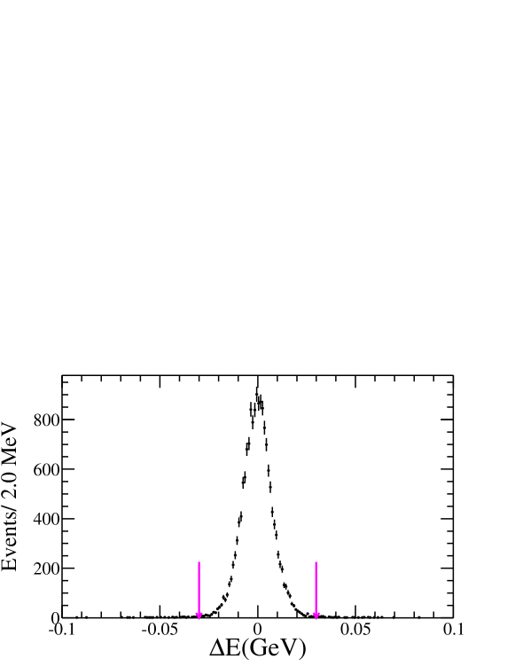
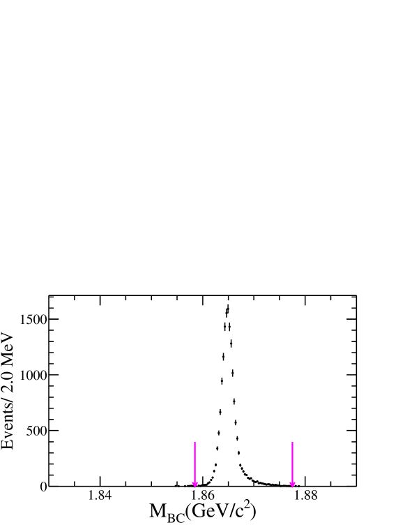
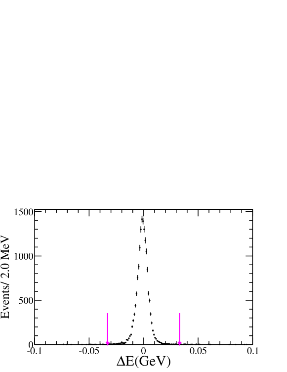
We require GeV for the final state,
GeV for the final state
and GeV/
for both of them. The corresponding and of selected candidate
are shown in Fig. 1, where the background is negligible.
Figure 1: Distributions of data for [(a) and (c)] and
[(b) and (d)] in side [(a) and (b)]
and in side [(c) and (d)]. The arrows indicate the selection criteria.
In each plot, all selection criteria described in this section
have been applied except the one on the variable.
To ensure the meson is on shell and improve the resolution,
the selected candidate events are further
subjected to a five-constraint (5C) kinematic fit, which constrains the
total four-momentum of all final state particles to the initial four-momentum of the system,
and the invariant mass of signal side
constrains to the mass in PDG PDG .
We discard events with a of the 5C kinematic fit larger than .
In order to suppress the background of with
, which has the same final state
as our signal decay, we perform a vertex constrained fit on any
pair in the signal side if the invariant mass falls into the mass window
GeV/
( is the nominal mass PDG ),
and reject the event if the corresponding significance of decay length
( the distance of the decay vertex to IP) is larger than 2.
The veto eliminates about 80% background
while retaining about 99% of signal events.
After applying all selection criteria, 15912 candidate events are obtained with a purity of 99.4,
as estimated by MC simulation.
The MC studies indicate that the dominant background arises from the
decay, the corresponding
produced number of events is estimated according to
(3)
where is the production
of
with and ,
is the signal yield with background subtracted
but without efficiency correction applied and is the corresponding efficiency obtained
from the SIGNAL MC sample, which is generated according to the results of fit to data
whose peaking background estimated from the generic MC sample.
and
are the branching fractions for and
, respectively, which are quoted from the PDG PDG .
According to Eq. (LABEL:Num_KsKPi), the number
of peaking background events () is estimated to be .
All other backgrounds from , and non-
decays are studied with the generic MC sample.
Their total contribution is estimated to be less than ten events, of which 5.5 and 2.0 are
from the decays and the non- decays, respectively.
These backgrounds are neglected in the following analysis and their effect is considered as a systematic
uncertainty, as discussed in Sec. VI.0.2.
IV Amplitude Analysis
The decay modes which may contribute to the decay
are listed in Table 1,
where the symbols S, P, V, A, and T denote a scalar,
pseudoscalar, vector, axial-vector, and tensor state, respectively.
The letters , , and in square brackets refer to the relative
angular momentum between the daughter particles.
The amplitudes and the relative phases between the different decay modes
are determined with a maximum likelihood fit.
IV.1 Likelihood function construction
The likelihood function is the product of the probability density function (PDF) of the observed events.
The signal PDF is given by
(4)
where is the detection efficiency parametrized in terms of the final four-momenta .
The index refers to the different particles in the final state.
is the standard element of the four-body phase space Zou , which is given by
(5)
is the total decay amplitude which is modeled as a
coherent sum over all contributing amplitudes
(6)
where the complex coefficient ( and
are the magnitude and phase for the amplitude, respectively)
and describe the relative contribution and the dynamics of the amplitude.
In four-body decays, the intermediate amplitude can be
a quasi-two-body decay or a cascade decay amplitude, and is given by
(7)
where the indices 1 and 2 correspond to the two intermediate resonances.
Here, and ()
are the propagator and the Blatt-Weisskopf barrier
factor Blatt , respectively, and
is the Blatt-Weisskopf barrier factor of the
decay.
The parameters and in the propagators are the invariant masses of the corresponding systems.
For nonresonant states with orbital angular momentum between the daughters,
we set the propagator to unity, which can be regarded as a very broad resonance.
The spin factor is constructed with the covariant tensor formalism Zou .
In practice, the presence of the two mesons imposes a
Bose symmetry in the final state.
This symmetry is explicitly accounted for in the amplitude by
exchange of the two pions with the same charge.
The contribution from the background is subtracted in the
likelihood calculation by assigning a negative weight to the background events
(8)
where is the number of candidate events in data,
and are the weight and
the number of events from the background MC sample, respectively.
In the nominal fit, only the peaking background
is considered, and the weight is
fixed to .
and are the four-momenta of the
final particle in the event of the data sample and in the
event of the background MC sample, respectively.
The normalization integral is determined by a MC technique taking into account the difference of detector
efficiencies for PID and tracking between data and MC simulation.
The weight for a given MC event is defined as
(9)
where and are the PID or
tracking efficiencies for charged tracks as a function of for the data and MC sample, respectively.
The efficiencies and are determined by studying the
sample for data and the MC sample respectively.
The MC integration is then given by
(10)
where is the index of the event of the MC sample and
is the number of the selected MC events.
is the PDF function used to generate the MC samples in MC integration.
In the numerator of Eq. (4), is independent of the fitted variables,
so it is regarded as a constant term in the fit.
IV.1.1 Spin factors
Due to the limited phase space available in the decay, we only consider the states with angular momenta up to 2.
As discussed in Ref. Zou , we define the spin projection operator
for a process
as
(11)
for spin 1,
(12)
for spin 2.
The covariant tensors for the final states of pure orbital
angular momentum are constructed from relevant momenta , , Zou
(13)
where .
Ten kinds of decay modes used in the analysis are listed in Table 1.
We use to represent the
decay from the meson and
to represent the decay from the intermediate state.
Table 1: Spin factors for different decay modes.
Decay mode
, ,
, ,
, ,
,
,
,
, ,
,
,
, ,
IV.1.2 Blatt-Weisskopf barrier factors
The Blatt-Weisskopf barrier factor Blatt is
a function of the angular momentum and the four-momenta
of the daughter particles.
For a process ,
the magnitude of the momentum of the daughter or in the rest system of is given by
(14)
with .
The Blatt-Weisskopf barrier factor is then given by
(15)
where . is the effective radius of the barrier, which is fixed to
for intermediate resonances and
for the meson.
is given by
(16)
(17)
(18)
IV.1.3 Propagator
The resonances and are parametrized
as relativistic Breit-Wigner function with
a mass depended width
(19)
where is the mass of resonance to be determined. is given by
(20)
where denotes the value of at .
The is parametrized as a relativistic Breit-Wigner function with a constant width
, and the is parametrized with the Gounaris-Sakurai line shape GS ,
which is given by
(21)
where
(22)
and the function is defined as
(23)
with
(24)
where is the charged pion mass.
The normalization condition at fixes the parameter .
It is found to be GS
(25)
IV.1.4 Parametrization of the -wave
For the -wave [denoted as ], we use the same parametrization as KPiS ,
which is extracted from scattering data LASS .
The model is built from a Breit-Wigner shape for the combined with an effective
range parametrization for the nonresonant component given by
(26)
with
(27)
(28)
where and denote the scattering length and effective interaction length.
and are the relative magnitudes (phases) for
the nonresonant and resonant terms, respectively.
and are defined as in Eq. (14) and Eq. (20), respectively.
In the fit, the parameters , , , , , , and
are fixed to the values obtained from the fit to the
Dalitz plot KPiS ,
as summarized in Table 2.
These fixed parameters will be varied within their uncertainties to estimate the corresponding
systematic uncertainties, which is discussed in detail in Sec. VI.0.1.
Table 2: -wave parameters,
obtained from the fit to the
Dalitz plot from KPiS .
(GeV/)
(GeV/)
(fixed)
IV.2 Fit fraction and the statistical uncertainty
We divide the fit model into several components according to the intermediate resonances,
which can be found in Sec. V.
The fit fractions of the individual components (amplitudes) are calculated according to the
fit results and are compared to other measurements.
In the calculation, a large phase space (PHSP) MC sample with neither detector acceptance nor resolution involved is used.
The fit fraction for an amplitude or a component (a certain subset of amplitudes) is defined as
(29)
where is either the amplitude
[]
or the component of a coherent sum of amplitudes
[],
is the number of the PHSP MC events.
To estimate the statistical uncertainties of the fit fractions,
we repeat the calculation of fit fractions by
randomly varying the fitted parameters according to the error matrix.
Then, for every amplitude or component, we fit the resulting distribution with a Gaussian function,
whose width gives the corresponding statistical uncertainty.
IV.3 Goodness of fit
To examine the performance of the fit process, the goodness of fit is
defined as follows.
Since the and all four final states particles have spin zero, the phase space of the decay
can be completely described by five
linearly independent Lorentz invariant variables.
Denoting as the one of the two identical pions which results in a higher
invariant mass
and the other pion as , we choose the five invariant masses
, ,
, and
.
To calculate the goodness of fit, the five-dimensional phase space is
first divided into cells with
equal size. Then, adjacent cells are combined until the number of events in each cell is larger than 20.
The deviation of the fit in each cell is calculated, ,
and the goodness of fit is quantified as ,
where and are the number of the observed events and
the expected number determined from the fit results in the cell, respectively,
and is the total number of cells.
The number of degrees of freedom (NDF) is given by , where
is the number of the free parameters in the fit.
V Results
In order to determine the optimal set of amplitude that contribute to
the decay ,
considering the results in PDG PDG ,
we start with the fit including the components with significant contribution
and add more amplitude in the fit one by one.
The corresponding statistical significance for the new amplitude is calculated with the change of the
log-likelihood value , taking the change of the degrees of
freedom into account.
In the and invariant mass spectra, there are
clear structures for and .
The intermediate resonance is observed
with or .
In the invariant mass spectrum, a broad bump appears.
We find this bump can be fitted as , which was also
observed by the Mark III MarKIII experiment.
If it is fitted with a nonresonant amplitude instead, we find that the significance for
with respect to is larger than .
The three-body nonresonant states come from two kinds of
contributions, and .
The
can be in a pseudoscalar, a vector or an axial-vector state, while
the can be in a scalar state.
The four-body nonresonant states are relatively complex, such as
VV, VS, TS, TV,
AP with VP or SP, all of which may contribute to the decay.
Since the process ,
has the largest fit fraction,
we fix the corresponding magnitude and phase to and and allow the
magnitudes and phases of the other processes to vary in the fit.
We keep the processes with significance larger than for the next iteration.
The fit involving both the
and the nonresonant contribution
does not result in a significantly improvement of fit,
but the fit fractions of the two amplitudes are much different
with the assumption of only and are nearly 100% correlated.
We avoid this kind of case and only consider the resonant term,
in agreement with the analysis of Mark III MarKIII .
For the process with
,
the corresponding significance is found to be only,
but we still include it in the fit
since the corresponding -wave process is found to have
a statistical significance of larger than .
Better projections in the invariant mass spectra
and an improved fit quality are also seen with this -wave process included.
Finally, we retain 23 processes categorized into seven components.
The other processes, not used in our nominal results but have been tested when determining
the nominal fit model, are listed in Appendix A.
The widths and masses of and are determined by the fit.
The results of are listed in Table 3.
Table 3: Masses and widths of intermediate resonances and ,
the first and second uncertainties are statistical and systematic, respectively.
Resonances
Mass (MeV/)
Width (MeV/)
The has a small fit fraction, and
we fix its mass and width to the PDG values PDG .
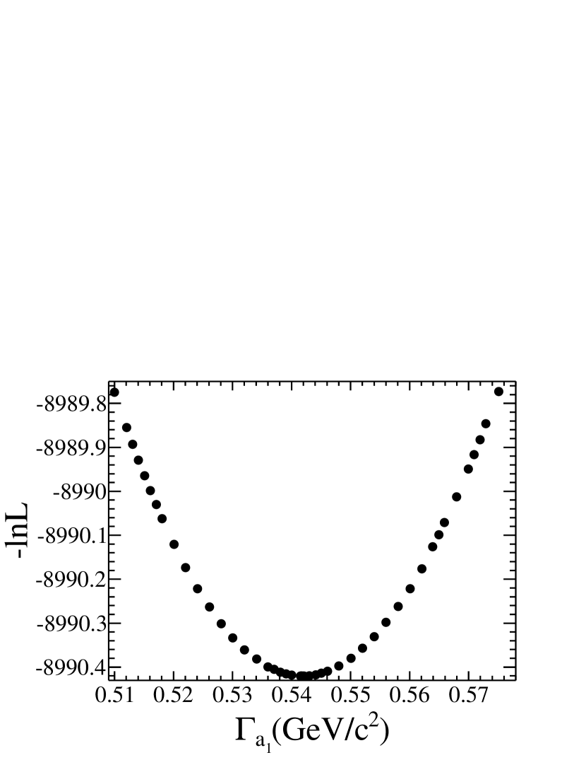
The has a mass close to the upper boundary of the
invariant mass spectrum.
Therefore, we determine its mass and width with a likelihood scan,
as shown in Fig. 2. The scan results are
(30)
where the uncertainties are statistical only.
The mass and width of are fixed to the scanned values in the nominal fit.
Figure 2: Likelihood scans of the width (a) and mass (b) of .
Our nominal fit yields a goodness of fit value of .
To calculate the statistical significance of a process, we repeat the fit process without the
corresponding process included, and the changes of log-likelihood value
and the number of free degree are taken into consideration.
The projections for eight invariant mass and the distribution of are shown in Fig. 3.
All of the components, amplitudes and the significance of amplitudes are listed in Table 4.
The fit fractions of all components are given in Table 5.
The phases and fit fractions of all amplitudes are given in Table 6.
Table 4: Statistical significances for different amplitudes.
Component
Amplitude
Significance ()
,
,
,
,
,
,
,
,
,
Table 5: Fit fractions for different components.
The first and second uncertainties are statistical and systematic, respectively.
Component
Fit fraction (%)
Mark III’s result
E691’s result
-
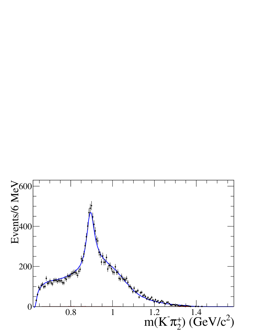
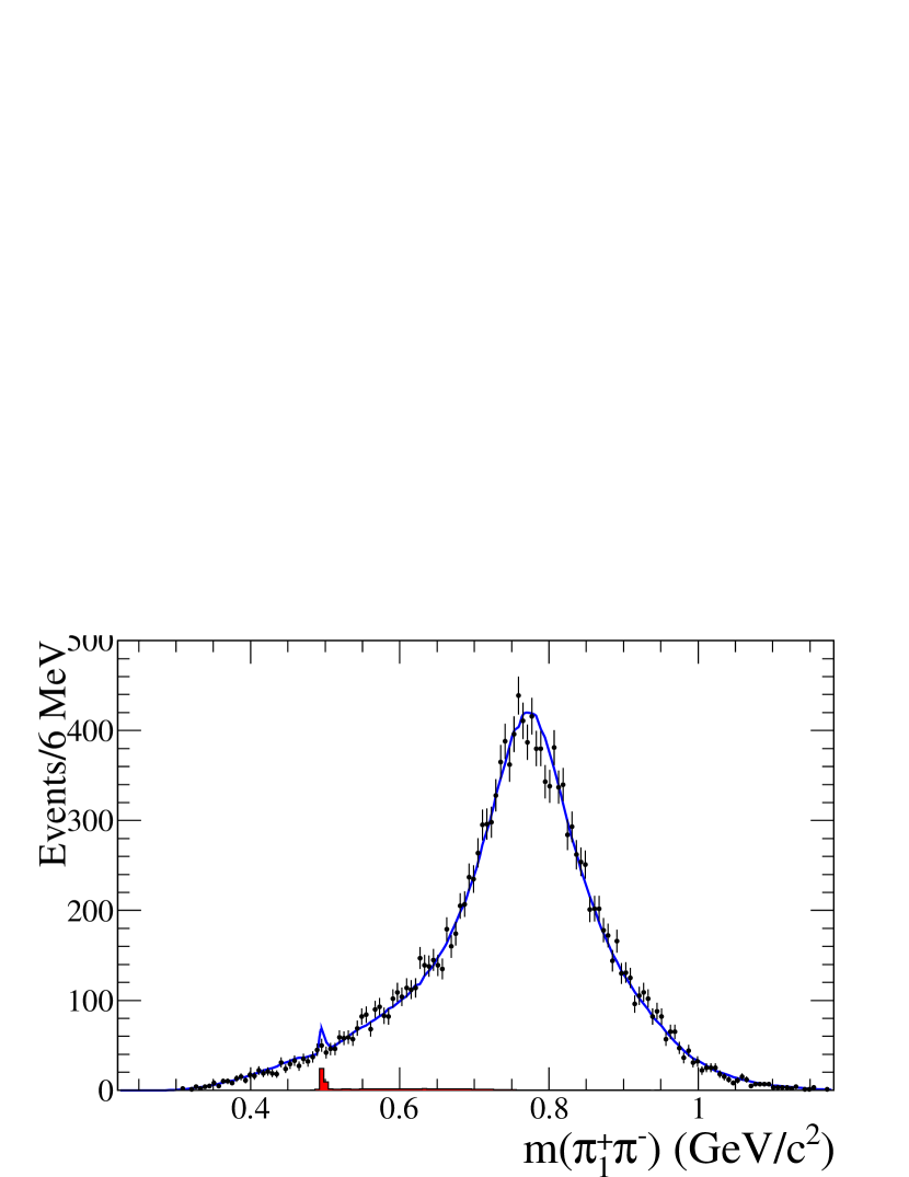
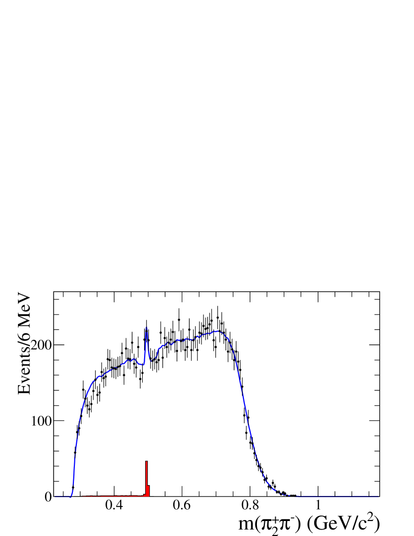
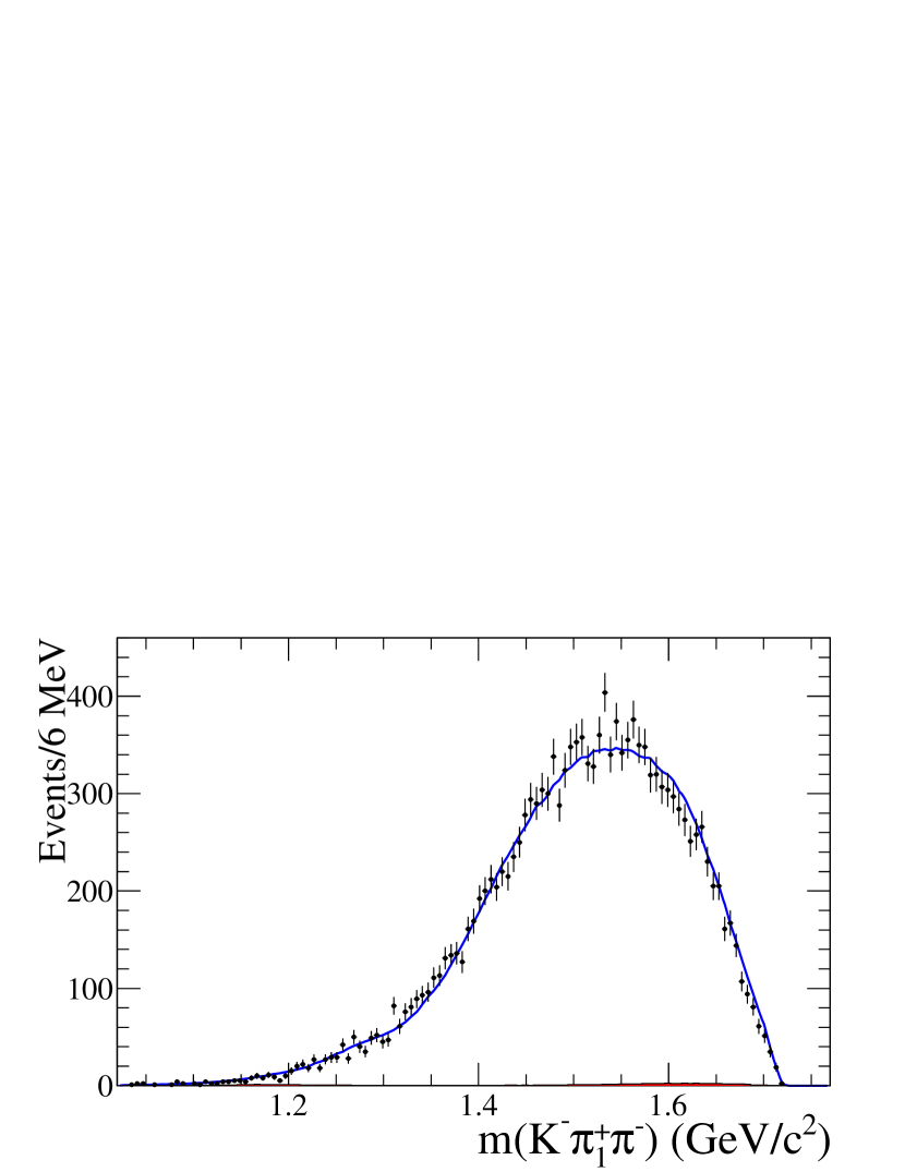
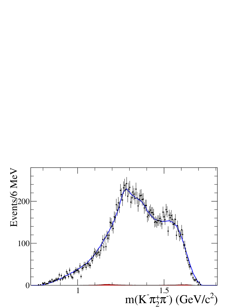
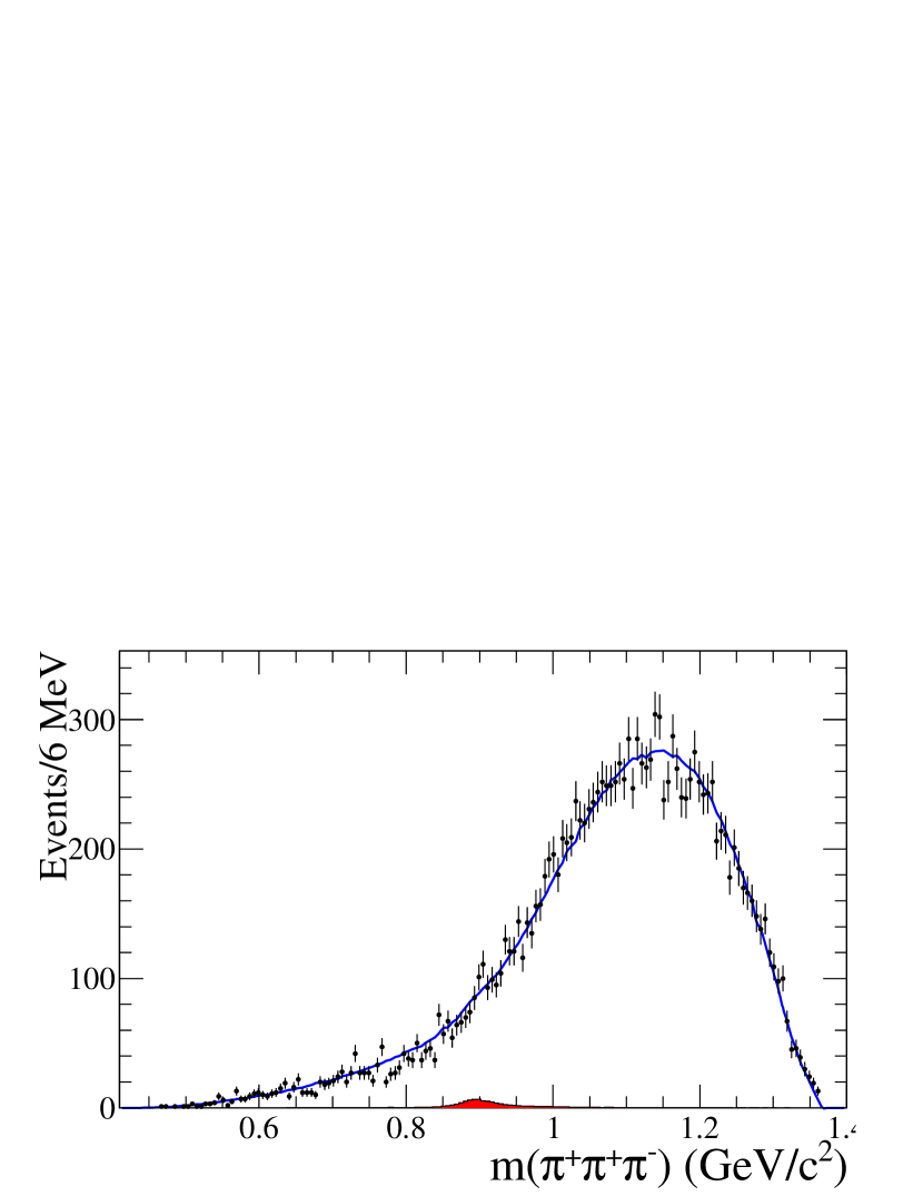
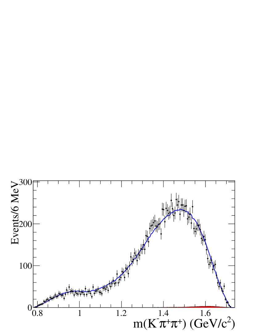
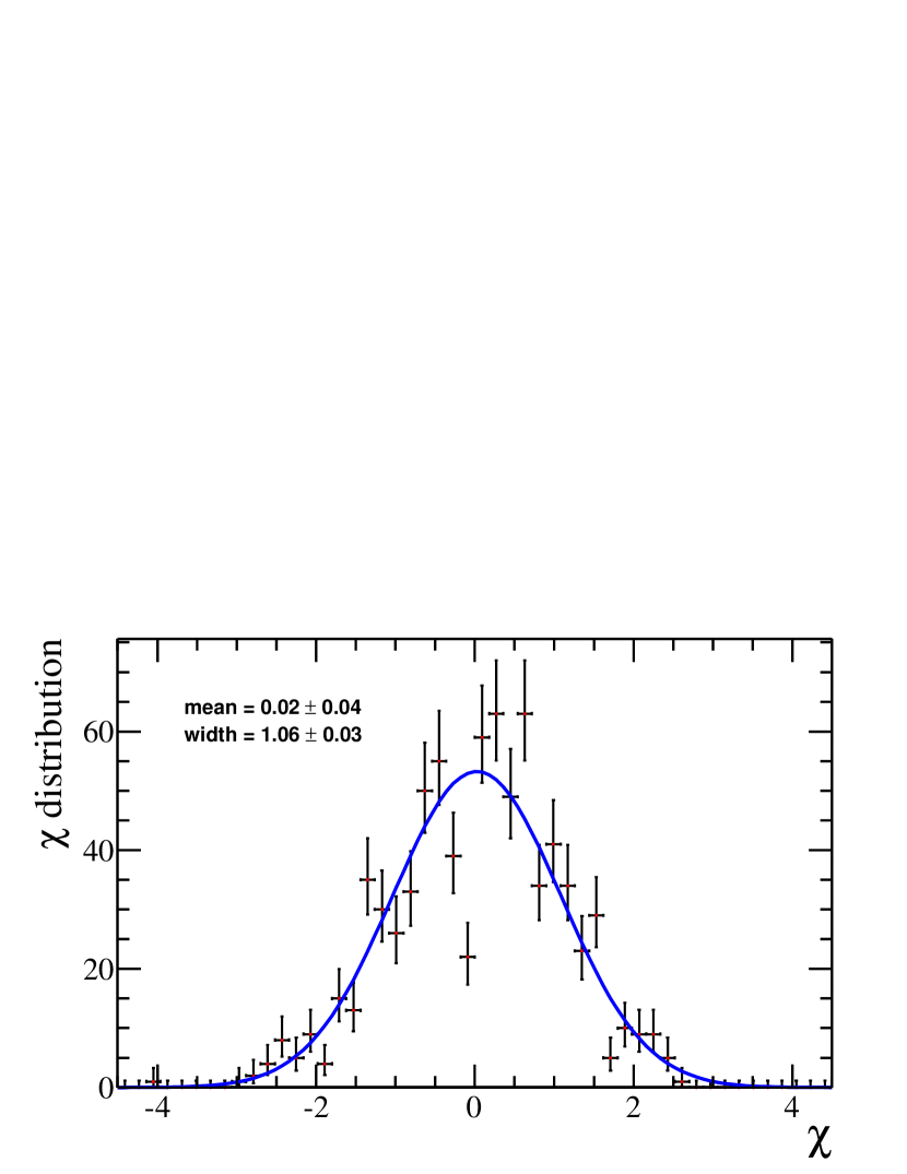
Figure 3:
Distribution of (a) , (b) , (c) ,
(d) , (e) , (f) ,
(g) and (h) ,
where the dots with error are data, and curves are for the fit projections.
The small red histograms in each projection shows the
peaking background. In (d), a peak of can be seen, which is consistent with the MC expectation.
The dip around the peak is caused by the requirements used to suppress the
background.
Plot (i) shows the fit (curve) to the distribution of the
(points with error bars) with a Gaussian function and the fitted values of the parameters (mean and width of Gaussian).
Table 6: Phases and fit fractions for different amplitudes.
The first and second uncertainties are statistical and systematic, respectively.
Amplitude
Fit fraction (%)
,
(fixed)
,
,
,
,
,
VI Systematic Uncertainties
The source of systematic uncertainties are divided into four categories:
(I) amplitude model, (II) background estimation,
(III) experimental effects and (IV) fitter performance.
The systematic uncertainties of the free parameters in the fit
and the fit fractions due to different contributions
are given in units of the statistical standard deviations
in Tables 7–9.
These uncertainties are added in quadrature, as they are uncorrelated,
to obtain the total systematic uncertainties.
Table 7: Systematic uncertainties on masses and widths of
intermediate resonances and .
Parameter
Source ()
total ()
I
II
III
IV
2.21
0.04
0.13
0.10
2.22
0.87
0.05
0.17
0.07
0.89
2.37
0.08
0.12
0.08
2.37
1.16
0.04
0.11
0.12
1.17
Table 8: Systematic uncertainties on fit fractions for different components.
Fit fraction
Source ()
total ()
I
II
III
IV
1.12
0.06
0.11
0.08
1.13
1.32
0.09
0.12
0.06
1.33
1.41
0.02
0.12
0.10
1.42
1.58
0.04
0.23
0.06
1.60
2.22
0.10
0.12
0.15
2.23
1.32
0.08
0.13
0.10
1.34
0.94
0.10
0.09
0.12
1.00
Table 9: Systematic uncertainties on phases and fit fractions for different amplitudes.
Source ()
total ()
I
II
III
IV
2.96
0.04
0.14
0.13
2.97
1.98
0.04
0.11
0.12
1.98
1.78
0.03
0.18
0.09
1.79
,
1.38
0.02
0.09
0.09
1.39
,
1.10
0.07
0.10
0.09
1.11
,
1.61
0.06
0.11
0.06
1.62
,
3.61
0.03
0.09
0.13
3.62
1.28
0.06
0.14
0.09
1.29
0.92
0.10
0.10
0.07
0.93
2.46
0.06
0.10
0.09
2.47
0.74
0.01
0.09
0.08
0.75
1.82
0.03
0.09
0.06
1.82
1.07
0.04
0.12
0.11
1.08
1.00
0.02
0.10
0.18
1.02
4.78
0.15
0.12
0.07
4.79
2.69
0.13
0.10
0.07
2.70
6.27
0.04
0.10
0.12
6.27
3.28
0.06
0.09
0.06
3.28
2.59
0.09
0.10
0.10
2.60
3.07
0.09
0.10
0.18
3.08
0.81
0.04
0.12
0.06
0.82
3.11
0.06
0.11
0.16
3.19
Fit fraction
Source ()
total ()
I
II
III
IV
1.76
0.04
0.09
0.10
1.77
0.27
0.02
0.09
0.12
0.31
1.79
0.06
0.12
0.17
1.80
,
1.48
0.10
0.12
0.07
1.45
,
0.93
0.04
0.09
0.06
0.94
,
1.01
0.05
0.11
0.16
1.03
,
1.12
0.03
0.12
0.13
1.14
,
1.58
0.04
0.23
0.06
1.60
1.38
0.08
0.09
0.09
1.39
0.93
0.06
0.09
0.16
0.95
2.81
0.09
0.11
0.09
2.82
0.69
0.03
0.09
0.06
0.70
0.93
0.06
0.09
0.16
0.95
1.06
0.05
0.09
0.20
1.08
0.60
0.02
0.00
0.10
0.61
3.10
0.07
0.09
0.06
3.10
1.14
0.08
0.10
0.07
1.15
1.29
0.12
0.10
0.12
1.30
1.73
0.07
0.09
0.07
1.73
2.08
0.12
0.10
0.07
2.09
3.54
0.05
0.10
0.11
3.54
0.87
0.07
0.11
0.07
0.88
0.99
0.09
0.10
0.08
1.01
VI.0.1 Amplitude model
Three sources are considered for the systematic uncertainty due to the amplitude model: the
masses and widths of the and the , the barrier effective radius
and the fixed parameters in the -wave model.
The uncertainty associated with the mass and width of and the are
estimated by varying the corresponding masses and widths
with 1 of errors quoted in PDG PDG , respectively.
The uncertainty related to the barrier effective radius is estimated by varying within
for the intermediate resonances and
for the in the fit.
The uncertainty from the input parameters of the -wave model are evaluated by varying the input values
within their uncertainties.
All the change of the results with respect to the nominal one are taken as the systematic uncertainties.
VI.0.2 Background estimation
The sources of systematic uncertainty related to the background include the amplitude and shape of
the background , and the
other potential backgrounds.
The uncertainties related to the background is
estimated by varying the number of background events within 1 of uncertainties and changing the shape
according to the uncertainties in PDF parameters from CLEO KsKPi .
The uncertainty due to the the other potential background is estimated by including the corresponding
background (estimated from generic MC sample) in the fit.
VI.0.3 Experimental effects
The uncertainty related to the experimental effects includes two separate components:
the acceptance difference between MC simulations and data caused by tracking and PID efficiencies,
and the detector resolution.
To determine the systematic uncertainty due to tracking and PID efficiencies,
we alter the fit by shifting the in Eq. (9)
within its uncertainty, and the changes of the nominal results
is taken as the systematic uncertainty.
The uncertainty caused by resolution is determined as the difference
between the pull distribution results obtained from simulated data using
generated and fitted four-momenta, as described in Sec. VI.0.4.
VI.0.4 Fitter performance
The uncertainty from the fit process is evaluated by studying toy MC samples.
An ensemble of 250 sets of SIGNAL MC samples with a size equal to the data sample are generated according to the
nominal results in this analysis.
The SIGNAL MC samples are fed into the event selection, and the same amplitude analysis is performed
on each simulated sample. The pull variables, , are
defined to evaluate the corresponding uncertainty, where is the input value
in the generator, and are the output value and the corresponding
statistical uncertainty, respectively.
The distribution of pull values for the 250 sets of sample are expected to be a normal Gaussian distribution,
and any shift on mean and widths indicate the bias on the fit values and its
statistical uncertainty, respectively.
Small biases for some fitted parameters
and fit fractions are observed. For the pull mean,
the largest bias is about 19% of a statistical uncertainty with a
deviation of about 3.0 from zero. For the pull width, the largest shift
is , about 3.0 standard deviations from 1.0.
We add in quadrature the mean and the mean error
in the pull and multiply this number with the statistical error to get the systematic error.
The fit results are given in Tables 1212.
The uncertainties in Tables 1212 are the statistical uncertainties of the
fits to the pull distributions.
Table 10: Pull mean and pull width of the pull distributions for the fitted masses and
widths of intermediate resonances and from
simulated data using either the generated or fitted four-momenta.
Parameter
Generated
Fitted
pull mean
pull width
pull mean
pull width
Table 11: Pull mean and pull width of the pull distributions for the different components from
simulated data using either the generated or fitted four-momenta.
Fit fraction
Generated
Fitted
pull mean
pull width
pull mean
pull width
Table 12: Pull mean and pull width of the pull distributions
for the phases and fit fractions of different amplitudes,
from simulated data using either the generated or fitted four-momenta.
Generated
Fitted
pull mean
pull width
pull mean
pull width
,
,
,
,
Fit fraction
Generated
Fitted
pull mean
pull width
pull mean
pull width
,
,
,
,
,
VII Conclusion
An amplitude analysis of the decay has been performed with the 2.93
of collision data at the resonance collected by the BESIII detector.
The dominant components,
, ,
four-body nonresonant decay and three-body nonresonant
improve upon the earlier results from Mark III and are
consistent with them within corresponding uncertainties.
The resonance observed
by Mark III is also confirmed in this analysis.
The detailed results are listed in Table 5.
About 40% of components comes from the nonresonant four-body ()
and three-body ( and )
decays. A detailed study considering the different orbital angular momentum is performed,
which was not included in the analyses of Mark III and E691. An
especially interesting process involving the
S-wave is described by an effective range parametrization.
By using the inclusive branching fraction
taken from the PDG PDG
and the fit fraction for the different components obtained in this analysis,
we calculate the exclusive absolute branching fractions for the individual components with
.
The results are summarized in Table 13 and are compared with the values quoted in PDG.
Our results have much improved precision; they may shed light in a
theoretical calculation.
The knowledge of
and
increase our understanding of the decay and ,
both of which are lacking in experimental measurements, but have large contributions to the decays.
Furthermore, knowledge of the submodes in the decay
will improve the determination of the reconstruction efficiency
when this mode is used to tag the as part of other measurements, like measurements of
branching fractions, the strong phase or the angle .
Table 13: Absolute branching fractions of the seven components and the
corresponding values in the PDG. Here, we denote and
.
The first two uncertainties are statistical and systematic, respectively.
The third uncertainties are propagated from the uncertainty of
.
Component
Branching fraction (%)
PDG value (%)
Acknowledgements.
The BESIII collaboration thanks the staff of BEPCII
and the IHEP computing center for their strong support.
This work is supported in part by National Key Basic Research Program
of China under Contract No. 2015CB856700;
National Natural Science Foundation of China (NSFC) under Contracts
No. 11075174, No. 11121092, No. 11125525, No. 11235011, No. 11322544, No. 11335008, No. 11375221, No. 11425524, No. 11475185, No. 11635010;
the Chinese Academy of Sciences (CAS) Large-Scale Scientific Facility Program;
Joint Large-Scale Scientific Facility Funds of the NSFC and CAS under Contracts
No. 11179007, No. U1232201, No. U1332201;
CAS under Contracts No. KJCX2-YW-N29, No. KJCX2-YW-N45;
100 Talents Program of CAS;
INPAC and Shanghai Key Laboratory for Particle Physics and Cosmology;
German Research Foundation DFG under Contract No. Collaborative Research Center CRC-1044;
Istituto Nazionale di Fisica Nucleare, Italy;
Ministry of Development of Turkey under Contract No. DPT2006K-120470;
Russian Foundation for Basic Research under Contract No. 14-07-91152;
U. S. Department of Energy under Contracts
No. DE-FG02-04ER41291, No. DE-FG02-05ER41374, No. DE-FG02-94ER40823, No. DESC0010118;
U.S. National Science Foundation;
University of Groningen (RuG) and the Helmholtzzentrum fuer Schwerionenforschung GmbH (GSI), Darmstadt;
WCU Program of National Research Foundation of Korea under Contract No. R32-2008-000-10155-0.
VIII Appendix A: Amplitudes Tested
The amplitudes listed below are tested when determining the nominal fit model,
but not used in our final fit result.
Cascade amplitudes
, -wave
, and -waves
,
,
,
Quasi-two-body amplitudes
Three-body amplitudes
, - and -waves
, and -waves
, and -waves
Four-body nonresonance amplitudes
- and -waves
- and -waves
- and -waves
References
(1) C. Patrignani et al. (Particle Data Group), Chin. Phys. C 40, 100001 (2016).
(2) G. Bonvicini et al. (CLEO Collaboration), Phys. Rev. D 89, 072002 (2014).
(3) D. Atwood, I. Dunietz and A. Soni, Phys. Rev. Lett. 78, 3257 (1997).
(4) S. Harnew and J. Rademacker, J. High Energy Phys. 03 (2015) 169.
(5) A. F. Falk, Y. Grossman, Z. Ligeti and A. A. Petrov, Phys. Rev. D 65, 054034 (2002).
(6) H. Y. Cheng and C. W. Chiang, Phys. Rev. D 81, 114020 (2010).
(7) D. Coffman et al. (Mark III Collaboration), Phys. Rev. D 45, 2196 (1992).
(8) J. C. Anjos et al. (E691 Collaboration), Phys. Rev. D 46, 1941 (1992).
(9) M. Ablikim et al. (BESIII Collaboration), Chin. Phys. C 37, 123001 (2013).
(10) M. Ablikim et al. (BESIII Collaboration), Phys. Lett. B 753, 629 (2016).
(11) B. S. Zou and D. V. Bugg, Eur. Phys. J. A 16, 537 (2003).
(12) M. Ablikim et al. (BESIII Collaboration), Nucl. Instrum. Methods Phys. Res., Sect. A 614, 345 (2010).
(13) S. Agostinelli et al. (GEANT4 Collaboration), Nucl. Instrum. Methods Phys. Res., Sect. A 506, 250 (2003).
(14) S. Jadach, B. F. L. Ward, and Z. Was, Phys. Rev. D 63, 113009 (2001).
(15) E. Barberio and Z. Was, Comput. Phys. Commun. 79, 291 (1994).
(16) D. J. Lange, Nucl. Instrum. Methods Phys. Res., Sect. A 462, 152 (2001);
R. G. Ping, Chin. Phys. C 32, 599 (2008).
(17) J. C. Chen et al., Phys. Rev. D 62, 034003 (2000).
(18) J. Insler et al. (CLEO Collaboration), Phys. Rev. D 85, 092016 (2012).
(19) S. U. Chung, Phys. Rev. D 48, 1225 (1993); 57, 431 (1998);
F. von Hippel and C. Quigg, Phys. Rev. D 5, 624 (1972).
(20) G. J. Gounaris and J. J. Sakurai, Phys. Rev. Lett. 21, 244 (1968).
(21) B. Aubert et al. ( Collaboration), Phys. Rev. D 78, 034023 (2008).
(22) D. Aston et al. (LASS Collaboration), Nucl. Phys. B296, 493 (1998).