Three-body halo states in effective field theory

Abstract

In this paper we study the renormalization of Halo effective field theory applied to the Helium-6 halo nucleus seen as an $\alpha$-neutron-neutron three-body state. We include the $0^{+}$ dineutron channel together with both the $3/2^{-}$ and $1/2^{-}$ neutron-$\alpha$ channels into the field theory and study all of the six lowest-order three-body interactions that are present. Furthermore, we discuss three different prescriptions to handle the unphysical poles in the P-wave two-body sector. In the simpler field theory without the $1/2^{-}$ channel present we find that the bound-state spectrum of the field theory is renormalized by the inclusion of a single three-body interaction. However, in the field theory with both the $3/2^{-}$ and $1/2^{-}$ included, the system can not be renormalized by only one three-body operator.

1 Introduction

Effective field theory (EFT) has become a widely used tool to construct interactions for few-body problems in atomic and nuclear physics. Examples are the nucleon-nucleon interaction constructed using Chiral EFT Epelbaum et al (2009); Machleidt and Entem (2011) and the atom-atom interaction for systems with a large scattering length Braaten and Hammer (2006); Hammer et al (2013). The properties of the corresponding three-body systems are usually obtained by the solution of the Faddeev equation. Halo nuclei Tanihata et al (1985); Jonson (2004) have become another arena for the application of EFTs. These are systems of tightly bound cores with weakly bound valence nucleons that can be found close to the neutron and proton driplines. Halo EFT uses the ratio of the valence-nucleon separation energy and the binding of the core as the expansion parameter for the low-energy EFT expansion. The core and valence nucleons are then the effective degrees of freedom used within this approach and the complexity of the problem is significantly reduced. An advantage of this approach is that the uncertainties of the model can be systematically reduced, by including more terms in the low-energy expansion.

Halo EFT has previously been applied to resonant two-body systems Bertulani et al (2002); Bedaque et al (2003); Higa et al (2008); Brown and Hale (2014), one-neutron halos Hammer and Phillips (2011); Rupak et al (2012); Acharya and Phillips (2013); Zhang et al (2014) and one-proton halos Ryberg et al (2014); Zhang et al (2014); Ryberg et al (2014, 2016). The ground state of Helium-6 has also been analyzed in Halo EFT, both by Rotureau and van Kolck Rotureau and van Kolck (2013) and by Ji, Elster and Phillips Ji et al (2014). Additional efforts on two-neutron halos can be found in Refs. Acharya et al (2013); Hagen et al (2013a, b).

One major tenet of EFTs is that observables have to be independent of any short-distance regulators. Such regulators have to be introduced to deal with the singularities that a low-momentum expansion typically introduces. One important consequence of this requirement is that operators frequently have to be promoted to lower order than naively expected from their mass dimension. One well-known example is the three-boson system where naive dimensional analysis implies that the three-body interaction should enter at N²LO. However, as was shown in an EFT treatment in Ref. Bedaque et al (1999) this interaction is needed already at LO for the theory to be renormalized.

Another problem that can occur in few-body systems is the appearance of spurious bound states in the two-body subsystem at cutoffs larger than the breakdown scale. This happens for example in the deuteron system when a chiral potential with a large momentum-space cutoff is employed, but also in Halo EFT when systems that interact resonantly in a relative P-wave are considered. For example, in the case of a low-lying P-wave two-body resonance one can fix the P-wave scattering length and effective range such that the two-body propagator reproduces this resonance. However, the denominator of such a propagator is then an order-three polynomial, which implies that additional two-body poles are present in the theory.

The Halo EFT analysis of the Helium-6 system is one example for which spurious bound states have become an immediate problem. The neutron-$\alpha$ interaction is resonant in the P-wave and the resulting two-body t-matrix has three poles in the complex plane with one of them being unphysical. In previous efforts it was suggested to remove the unitarity piece $ik^{3}$ from the denominator of the P-wave propagator, see Ref. Bedaque et al (2003). This prescription is possible if only one fine-tuning is assumed and it is restricted to LO. We propose and discuss two additional prescriptions.

In this paper, we derive (for the first time) the complete field-theoretical equations for the Helium-6 system from appropriate diagrammatics. The two-body sector is renormalized by fitting the low-energy constants to the resonance position and width of the Helium-5 system and the neutron-neutron scattering length. In Refs. Rotureau and van Kolck (2013); Ji et al (2014), the Helium-6 system was renormalized with the simplest possible three-body counterterm and an analysis of other possible operators was omitted. Here, we perform a renormalization analysis of the bound-state spectrum, using all of the six lowest-order three-body interactions that are present. We also compare the three different prescriptions of how to treat the unphysical P-wave poles in the two-body sector.

This manuscript is organized as follows: In Sec. 2, we discuss the EFT used to describe the Helium-6 system and its renormalization in the two-body sector. In Sec. 3 we analyze the renormalization of the three-body system. Finally, a conclusion is provided in Sec. 4.

2 Method

In this section, we present a framework for the treatment of the bound $0^{+}$ ground state of ${}^{6}\mathrm{He}$, which has a two-neutron separation energy of $1~{}\mathrm{MeV}$. It can be viewed as consisting of an $\alpha$ particle and two neutrons. The one-nucleon separation energy of the $\alpha$ particle is $20~{}\mathrm{MeV}$ and this defines the break-down scale in energy. Thus we have a good separation of scales. We include the S-wave dineutron channel and both the $3/2^{-}$ and $1/2^{-}$ channels of the P-wave neutron-$\alpha$ interaction. These two channels correspond to the two low-lying resonances of ${}^{5}\mathrm{He}$, with energy positions and widths $E^{(3/2^{-})}=0.798~{}\mathrm{MeV}$, $\Gamma^{(3/2^{-})}=0.648~{}\mathrm{MeV}$, $E^{(1/2^{-})}=2.07~{}\mathrm{MeV}$ and $\Gamma^{(1/2^{-})}=5.57~{}\mathrm{MeV}$, respectively Tilley et al (2002). We expect that the $3/2^{-}$ is more important than the $1/2^{-}$ channel, since it is lower in energy.

2.1 Lagrangian

The fields that are included in this field theory are the $1/2^{+}$ neutron, $n_{\sigma}$, the $0^{+}$ $\alpha$ core, $c$, the $0^{+}$ dineutron field, $b$, the ${}^{5}\mathrm{He}(3/2^{-})$ field, $d_{a}$, and the ${}^{5}\mathrm{He}(1/2^{-})$ field, $\tilde{d}_{\sigma}$. The spin indices are defined as $\sigma=-1/2,1/2$ and $a=-3/2,-1/2,1/2,3/2$. We will also use $\chi$ as a spin-$1/2$ and $b$ as a spin-$3/2$ index, together with $i,j=-1,0,1$ as spin-$1$ indices.

We write the Lagrangian for the $0^{+}$ channel of ${}^{6}\mathrm{He}$ as a sum of Lagrangian parts

$$\mathcal{L}=\mathcal{L}^{(1)}+\mathcal{L}^{(2)}+\mathcal{L}^{(3)}~{}.$$ (1)

The one-body part is given by

$$\mathcal{L}^{(1)}=c^{\dagger}\left[i\partial_{t}+\frac{\nabla^{2}}{8m}\right]c+n_{\sigma}^{\dagger}\left[i\partial_{t}+\frac{\nabla^{2}}{2m}\right]n_{\sigma}+\dots~{},$$ (2)

where the neutron, $n_{\sigma}$, has a mass $m$ and the core, $c$, has a mass $4m$. The dots refer to relativistic one-body corrections.

The two-body Lagrangian is given by

$$\mathcal{L}^{(2)}= d^{\dagger}_{a}\left[\Delta_{1}+\nu_{1}\left(i\partial_{t}+\frac{\nabla^{2}}{10m}\right)\right]d_{a}+g_{1}\mathcal{C}^{a}_{i\chi}\left[d^{\dagger}_{a}c\left(\frac{4}{5}i\overrightarrow{\nabla}_{i}-\frac{1}{5}i\overleftarrow{\nabla}_{i}\right)n_{\chi}+\mathrm{h.c.}\right]$$

$$+\tilde{d}^{\dagger}_{\sigma}\left[\tilde{\Delta}_{1}+\tilde{\nu}_{1}\left(i\partial_{t}+\frac{\nabla^{2}}{10m}\right)\right]\tilde{d}_{\sigma}+\tilde{g}_{1}\mathcal{C}^{\sigma}_{i\chi}\left[\tilde{d}^{\dagger}_{\sigma}c\left(\frac{4}{5}i\overrightarrow{\nabla}_{i}-\frac{1}{5}i\overleftarrow{\nabla}_{i}\right)n_{\chi}+\mathrm{h.c.}\right]$$

$$+b^{\dagger}\Delta_{0}b+\frac{1}{2}g_{0}\mathcal{C}^{0}_{\sigma\chi}\left(b^{\dagger}n_{\sigma}n_{\chi}+\mathrm{h.c.}\right)+\dots~{}.$$ (3)

The parameters $\Delta_{1}$, $\nu_{1}$ and $g_{1}$ define the neutron-$\alpha$ P-wave interaction in the $3/2^{-}$ channel and $\tilde{\Delta}_{1}$, $\tilde{\nu}_{1}$ and $\tilde{g}_{1}$ define the neutron-$\alpha$ P-wave interaction in the $1/2^{-}$ channel. The low-energy constants $\Delta_{0}$ and $g_{0}$ define the neutron-neutron S-wave interaction in the $0^{+}$ channel. We define the Clebsch-Gordan coefficients accoring to $\mathcal{C}^{a}_{i\chi}=\langle 1i\frac{1}{2}\chi|(1\frac{1}{2})\frac{3}{2}a\rangle$, $\mathcal{C}^{\sigma}_{i\chi}=\langle 1i\frac{1}{2}\chi|(1\frac{1}{2})\frac{1}{2}\sigma\rangle$ and $\mathcal{C}^{0}_{\sigma\chi}=\langle\frac{1}{2}\sigma\frac{1}{2}\chi|(\frac{1}{2}\frac{1}{2})00\rangle$. The derivative operators $(\frac{4}{5}i\overrightarrow{\nabla}_{i}-\frac{1}{5}i\overleftarrow{\nabla}_{i})$ ensure that the interactions are in the P-wave channel and that the Lagrangian obeys Galilean invariance. The dots refer to higher-order two-body interactions.

For the three-body part of the Lagrangian we have

$$\mathcal{L}^{(3)}= h_{1}\mathcal{C}^{0}_{a\chi i}\mathcal{C}^{0}_{a^{\prime}\chi^{\prime}i^{\prime}}\left(d_{a}^{\dagger}i\overleftrightarrow{\nabla}_{i}n_{\chi}^{\dagger}\right)\left(d_{a^{\prime}}i\overleftrightarrow{\nabla}_{i^{\prime}}n_{\chi^{\prime}}\right)$$

$$+h_{2}\mathcal{C}^{0}_{\sigma\chi i}\mathcal{C}^{0}_{a^{\prime}\chi^{\prime}i^{\prime}}\left[\left(\tilde{d}_{\sigma}^{\dagger}i\overleftrightarrow{\nabla}_{i}n_{\chi}^{\dagger}\right)\left(d_{a^{\prime}}i\overleftrightarrow{\nabla}_{i^{\prime}}n_{\chi^{\prime}}\right)+\mathrm{h.c.}\right]$$

$$+h_{3}\mathcal{C}^{0}_{\sigma\chi i}\mathcal{C}^{0}_{\sigma^{\prime}\chi^{\prime}i^{\prime}}\left(\tilde{d}_{\sigma}^{\dagger}i\overleftrightarrow{\nabla}_{i}n_{\chi}^{\dagger}\right)\left(\tilde{d}_{\sigma^{\prime}}i\overleftrightarrow{\nabla}_{i^{\prime}}n_{\chi^{\prime}}\right)$$

$$+h_{4}b^{\dagger}c^{\dagger}bc$$

$$+h_{5}\mathcal{C}^{0}_{a\chi i}\left[\left(d_{a}^{\dagger}i\overleftrightarrow{\nabla}_{i}n_{\chi}^{\dagger}\right)bc+\mathrm{h.c.}\right]$$

$$+h_{6}\mathcal{C}^{0}_{\sigma\chi i}\left[\left(\tilde{d}_{\sigma}^{\dagger}i\overleftrightarrow{\nabla}_{i}n_{\chi}^{\dagger}\right)bc+\mathrm{h.c.}\right]+\dots~{}.$$ (4)

Here we have defined the Galilean invariant P-wave interaction operators as $\overleftrightarrow{\nabla}=\frac{5}{6}\overrightarrow{\nabla}-\frac{1}{6}\overleftarrow{\nabla}$. The triple-subscript $\mathcal{C}$ objects are defined according to $\mathcal{C}^{0}_{a\chi i}=\mathcal{C}_{a\chi}^{j}\mathcal{C}_{ji}^{0}$ and $\mathcal{C}^{0}_{\sigma\chi i}=\mathcal{C}_{\sigma\chi}^{j}\mathcal{C}_{ji}^{0}$. The terms that we have included in this three-body Lagrangian part (4) are the lowest order interactions that are of scaling dimension $7$ (note that the p-wave dimer field has scaling dimension 1 and the dineutron field has scaling dimension 2). As such, they are expected to enter at N²LO. However, in order to achieve proper renormalization we need to promote at least one of them to LO. We will discuss this further in Sec. 3. Note that in previous treatments of ${}^{6}\mathrm{He}$ only the $h_{1}$ term has been considered Rotureau and van Kolck (2013); Ji et al (2014).

2.2 Two-body physics

We begin by considering the two-body sector of the field theory. This amounts to writing down the relevant dicluster propagators, that is the dineutron propagator and the ${}^{5}\mathrm{He}$ propagators for the $3/2^{-}$ and $1/2^{-}$ channels. We then discuss how to remove the unphysical pole of the P-wave propagators, using one of three prescriptions.

The dineutron subsystem

– For the neutron-neutron interaction we restrict ourselves to the S-wave interaction. This interaction has an unnaturally large scattering length, $a_{0}=-18.9~{}\mathrm{fm}$ Gårdestig (2009), which means that we must resum the interaction to infinite order. The resulting full LO dineutron propagator is therefore given by a geometric series, which we write in closed form as

$$iB(E,\mathbf{p})=\frac{i}{\Delta_{0}+\Sigma_{0}(E,\mathbf{p})}~{}.$$ (5)

The irreducible self-energy, $\Sigma_{0}$, is given by

$$\Sigma_{0}(E,\mathbf{p})=\frac{g_{0}^{2}m}{2\pi^{2}}\left[L_{1}-\frac{i\pi}{2}\sqrt{mE-\frac{\mathbf{p}^{2}}{4}}\right]~{},$$ (6)

with a divergence $L_{1}$, defined by

$$L_{n}=\int\mathrm{d}pp^{n-1}~{}.$$ (7)

This divergence is absorbed in the renormalization of the paramter $\Delta_{0}$. The scattering diagram is given in Fig. 1(a) where the double line defines the full dineutron propagator. The propagator (5) is given for a four-momentum $(E,\mathbf{p})$.

Figure 1: Elastic scattering in the two-body subsystems of ${}^{6}\mathrm{He}$. (a) The neutron-neutron scattering diagram. The full dineutron propagator is denoted by the double line. (b) The neutron-$\alpha$ elastic scattering diagram in the $3/2^{-}$ channel. The full ${}^{5}\mathrm{He}(3/2^{-})$ dicluster propagator is denoted by the double line with internal bottom-to-top right tilted lines. (c) The neutron-$\alpha$ elastic scattering diagram in the $1/2^{-}$ channel. The full ${}^{5}\mathrm{He}(1/2^{-})$ dicluster propagator is denoted by the double line with internal bottom-to-top left tilted lines.

By matching to ERE parameters, i.e. the neutron-neutron scattering length $a_{0}$, we write the full dineutron propagator as

$$B(E,\mathbf{p})=\frac{4\pi}{g_{0}^{2}m}\frac{1}{\frac{1}{a_{0}}+i\sqrt{m\left(E-\frac{\mathbf{p}^{2}}{4m}\right)}},$$ (8)

which is the expression that we will use in actual calculations.

The ${}^{5}\mathrm{He}$ subsystem

– For a P-wave interaction we need to also include the $\nu_{1}$ term of the Lagrangian part (3) to achieve proper renormalization. This term gives the effective range contribution. The LO full dicluster propagators for the P-wave $3/2^{-}$ channel is thus written as

$$iD(E,\mathbf{p})=\frac{i}{\Delta_{1}+\nu_{1}\left(E-\frac{\mathbf{p}^{2}}{10m}\right)+\Sigma_{1}(E,\mathbf{p})}~{},$$ (9)

where the irreducible self energy is given by

$$\Sigma(E,\mathbf{p})=\frac{4g_{1}^{2}m}{15\pi^{2}}\left[L_{3}+\left(\frac{8mE}{5}-\frac{4\mathbf{p}^{2}}{25}\right)L_{1}-\frac{i\pi}{2}\left(\frac{8mE}{5}-\frac{4\mathbf{p}^{2}}{25}\right)^{3/2}\right]~{}.$$ (10)

Note that the propagator (9) is written as a geometric series in closed form, similar to the dineutron propagator (5). In the P-wave irreducible self-energy (10) there are two independent divergences, given by the divergent integrals $L_{1}$ and $L_{3}$. In the renormalization of the parameters $\Delta_{1}$ and $g_{1}$ these divergent terms are absorbed, but one should note that this is the reason for why the effective range is needed at LO for the P-wave interaction to be properly renormalized. Matching the dicluster propagator (9) to the scattering t-matrix we can write the propagator using the ERE parameters, scattering length $a_{1}$ and effective range $r_{1}$, according to

$$D(E,\mathbf{p})=\frac{15\pi}{2mg_{1}^{2}}\frac{1}{\frac{1}{a_{1}}-\frac{1}{2}r_{1}\left(\frac{8mE}{5}-\frac{4\mathbf{p}^{2}}{25}\right)+i\left(\frac{8mE}{5}-\frac{4\mathbf{p}^{2}}{25}\right)^{3/2}}~{}.$$ (11)

The $3/2^{-}$ P-wave scattering diagram is given in Fig. 1(b) where we also define the $3/2^{-}$ dicluster propagator as the double line with internal bottom-to-top right-tilted lines.

The $1/2^{-}$ dicluster propagator is given in the same fashion as

$$\tilde{D}(E,\mathbf{p})=\frac{15\pi}{2m\tilde{g}_{1}^{2}}\frac{1}{\frac{1}{\tilde{a}_{1}}-\frac{1}{2}\tilde{r}_{1}\left(\frac{8mE}{5}-\frac{4\mathbf{p}^{2}}{25}\right)+i\left(\frac{8mE}{5}-\frac{4\mathbf{p}^{2}}{25}\right)^{3/2}}~{},$$ (12)

with $\tilde{a}_{1}$ and $\tilde{r}_{1}$ the corresponding scattering length and effective range, respectively. The $1/2^{-}$ scattering diagram is shown in Fig. 1(c), where the double line with internal bottom-to-top left-tilted lines defines the $1/2^{-}$ dicluster propagator.

We extract the ERE parameters for the P-wave channels by matching the ${}^{5}\mathrm{He}$ resonances to the pole positions of the dicluster propagators (11) and (12). The resulting values are $a_{1}=-76.12~{}\mathrm{fm}^{3}$, $r_{1}=-141.84~{}\mathrm{MeV}$, $\tilde{a}_{1}=-60.37~{}\mathrm{fm}^{3}$ and $\tilde{r}_{1}=66.87~{}\mathrm{MeV}$. Note however that the denominators of the dicluster propagators are given by third order polynomials. As such, there is also an unphysical pole for both the $3/2^{-}$ and $1/2^{-}$ channel. These poles need to be removed if we are to perform three-body calculations using such dicluster propagators.

We now turn to the discussion of three different prescriptions of how to handle the unphysical pole of a P-wave propagator. The first method we denote as the unitarity piece removal prescription (UP), since this presciption removes the $ik^{3}$ term in the denominator of the dicluster propagator. The reason for why this is permissable is that at low momentum the unitarity piece scales as $ik^{3}\sim k_{\mathrm{lo}}^{3}$ while the other two terms scale according to $1/a_{1}\sim k_{\mathrm{lo}}^{2}k_{\mathrm{hi}}\sim r_{1}k^{2}$, by assumption. Therefore, at LO, we may neglect the unitarity piece. Note however that this prescription is only valid if the scalings of the ERE parameters are as stated. Otherwise the unphysical pole must be handled in some other way. The resulting propagator in the UP is

$$D^{(\mathrm{UP})}(E,\mathbf{p})=\frac{15\pi}{2mg_{1}^{2}}\frac{1}{\frac{1}{a_{1}}-\frac{1}{2}r_{1}k^{2}}~{},$$ (13)

where $k=\sqrt{\frac{8mE}{5}-\frac{4\mathbf{p}^{2}}{25}}$. As can be seen, the UP has moved the physical pole to the real momentum axis. This change of the pole position should be within the bounds of the LO model. Moreover, note that the low-momentum physics of the UP propagator is unchanged up to order $k^{2}$.

The second method is the subtraction prescription (SP), where the unphysical pole is simply subtracted from the dicluster propagator. The SP propagator is given by

$$D^{(\mathrm{SP})}(E,\mathbf{p})=\frac{15\pi}{2mg_{1}^{2}}\frac{1}{\frac{1}{a_{1}}-\frac{1}{2}r_{1}k^{2}+ik^{3}}-\frac{\mathcal{R}_{0}}{k-k_{0}}~{},$$ (14)

where $k_{0}$ and $\mathcal{R}_{0}$ are the pole position and residue of the unphysical pole. There are two things to note about the SP: First, the prescription does not move the physical pole and, second, it changes the low-momentum physics. This second point means that the scattering length and effective range of the SP propagator (14) are not the same as before the subtraction. The impact of the subtraction depends on how deep the spurious bound state is but can typically considered to be of higher order.

The third prescription we call the expansion prescription (EP). In the EP we expand the unphysical pole to second order in momentum and therefore it does neither change the low-momentum physics, nor move the physical pole position. The EP propagator is given by

$$D^{(\mathrm{EP})}(E,\mathbf{p})= \frac{15\pi}{2mg_{1}^{2}}\frac{1}{\frac{1}{a_{1}}-\frac{1}{2}r_{1}k^{2}+ik^{3}}$$

$$-\mathcal{R}_{0}\left(\frac{1}{k-k_{0}}+\frac{1}{k_{0}}+\frac{k}{k_{0}^{2}}+\frac{k^{2}}{k_{0}^{3}}\right)~{}.$$ (15)

As can be seen in Eq. (15) this propagator has very different large-momentum asymptotics than the origanal dicluster propagator, since it now scales as $k^{2}$ for large $k$. From an EFT perspective this is not an issue, since the large-momentum asymptotics is renormalized. However, numerically we are limited to lower cutoffs in the EP, than in the UP or SP, since the three-body amplitudes will consist of differences of very large numbers when the cutoff is large.

2.3 Three-body scattering diagrams

In this part we write down the three-body integral equations for the $0^{+}$ channel of ${}^{6}\mathrm{He}$. We define the integral equations to have outgoing ${}^{5}\mathrm{He}(3/2^{-})$ and neutron legs. Since we have three two-body channels the integral equation is a coupled system with three parts: (i) The A-amplitude, with incoming ${}^{5}\mathrm{He}(3/2^{-})$ and neutron legs, (ii) the B-amplitude, with incoming ${}^{5}\mathrm{He}(1/2^{-})$ and neutron legs, and (iii) the C-amplitude, with incoming dineutron and $\alpha$-particle legs. Note that to in order to have a total $0^{+}$ the ${}^{5}\mathrm{He}$+neutron legs must be in a relative P-wave, while the dineutron+$\alpha$ legs must be in a relative S-wave. The three-body integral equations are shown in a diagramatic form in Fig. 2.

Figure 2: The three-body scattering diagrams. Since there are three two-body channels the scattering equation is given by a coupled integral equation of three parts. See text for details.

On the first line for each of the amplitudes in Fig. 2 the two inhomogeneous terms are shown. However, in this paper we are only concerned with bound-state solutions for which the scattering amplitude has a pole for negative energies. As such the inhomogeneous terms are not necessary for our purpose. We have constructed the integral equations from the diagrams in Fig. 2. The homogeneous part of the integral equations projected onto a total $0^{+}$ is given by

$$iA^{(A)}(k,p)= ig_{1}^{2}\frac{2m}{3\pi^{2}}\int\mathrm{d}qq^{2}K^{(AA)}(k,q)D\left(E-\frac{3q^{2}}{5m},0\right)A(q,p)$$ (16)

$$iA^{(B)}(k,p)= ig_{1}\tilde{g}_{1}\frac{2m}{3\pi^{2}}\int\mathrm{d}qq^{2}K^{(AB)}(k,q)\tilde{D}\left(E-\frac{3q^{2}}{5m},0\right)B(q,p)$$ (17)

$$iA^{(C)}(k,p)= ig_{1}g_{0}\frac{m}{\sqrt{6}\pi^{2}}\int\mathrm{d}qq^{2}K^{(AC)}(k,q)B\left(E-\frac{3q^{2}}{8m},0\right)C(q,p)$$ (18)

$$iB^{(A)}(k,p)= ig_{1}\tilde{g}_{1}\frac{2m}{3\pi^{2}}\int\mathrm{d}qq^{2}K^{(BA)}(k,q)D\left(E-\frac{3q^{2}}{5m},0\right)A(q,p)$$ (19)

$$iB^{(B)}(k,p)= i\tilde{g}_{1}^{2}\frac{2m}{3\pi^{2}}\int\mathrm{d}qq^{2}K^{(BB)}(k,q)\tilde{D}\left(E-\frac{3q^{2}}{5m},0\right)B(q,p)$$ (20)

$$iB^{(C)}(k,p)= i\tilde{g}_{1}g_{0}\frac{m}{\sqrt{6}\pi^{2}}\int\mathrm{d}qq^{2}K^{(BC)}(k,q)B\left(E-\frac{3q^{2}}{8m},0\right)C(q,p)$$ (21)

$$iC^{(A)}(k,p)= 2ig_{0}g_{1}\frac{m}{\sqrt{6}\pi^{2}}\int\mathrm{d}qq^{2}K^{(CA)}(k,q)D\left(E-\frac{3q^{2}}{5m},0\right)A(q,p)$$ (22)

$$iC^{(B)}(k,p)= 2ig_{0}\tilde{g}_{1}\frac{m}{\sqrt{6}\pi^{2}}\int\mathrm{d}qq^{2}K^{(CB)}(k,q)\tilde{D}\left(E-\frac{3q^{2}}{5m},0\right)B(q,p)$$ (23)

$$iC^{(C)}(k,p)= 2ig_{0}^{2}\frac{m}{2\pi^{2}}\int\mathrm{d}qq^{2}K^{(CC)}(k,q)B\left(E-\frac{3q^{2}}{8m}\right)C(q,p)~{}.$$ (24)

The momenta are defined such that the incoming fields have relative momentum $\mathbf{k}$ and the outgoing fields have relative momentum $\mathbf{p}$. The loop-momentum $q$ is limited by the cutoff $\Lambda$ and the integration span $[0,\Lambda]$ is replaced with a Legendre mesh when the integral equations are solved numerically.

The kernels $K^{XY}$, where $X,Y=A,B,C$, are defined as

$$K^{(AA)}(k,p)= \frac{27}{25}Q_{0}(\rho_{1}(k,p))+\frac{2}{5}\frac{k^{2}+p^{2}}{kp}Q_{1}(\rho_{1}(k,p))+Q_{2}(\rho_{1}(k,p))$$

$$-H_{1}\frac{kp}{\Lambda^{2}}$$ (25)

$$K^{(AB)}(k,p)= K^{(BA)}(k,p)$$

$$= \frac{\sqrt{2}}{25}Q_{0}(\rho_{1}(k,p))+\frac{\sqrt{2}}{5}\frac{k^{2}+p^{2}}{kp}Q_{1}(\rho_{1}(k,p))+\sqrt{2}Q_{2}(\rho_{1}(k,p))$$

$$-H_{2}\frac{kp}{\Lambda^{2}}$$ (26)

$$K^{(AC)}(k,p)= K^{(CA)}(p,k)$$

$$= \frac{4}{5p}Q_{0}(\rho_{2}(k,p))+\frac{1}{k}Q_{1}(\rho_{2}(k,p))-H_{5}\frac{k}{\Lambda^{2}}$$ (27)

$$K^{(BB)}(k,p)= \frac{26}{25}Q_{0}(\rho_{1}(k,p))+\frac{1}{5}\frac{k^{2}+q^{2}}{kq}Q_{1}(\rho_{1}(k,q))-H_{3}\frac{kp}{\Lambda^{2}}$$ (28)

$$K^{(BC)}(k,p)= K^{(CB)}(p,k)$$

$$= \frac{4}{5\sqrt{2}p}Q_{0}(\rho_{2}(k,p))+\frac{1}{\sqrt{2}k}Q_{1}(\rho_{2}(k,p))-H_{6}\frac{k}{\Lambda^{2}}$$ (29)

$$K^{(CC)}(k,p)= -H_{4}\frac{1}{\Lambda^{2}}~{},$$ (30)

where the arguments to the Legendre-Q functions $Q_{L}$ are given by

$$\rho_{1}(k,p)= \frac{4mE}{kp}-\frac{5k}{2p}-\frac{5p}{2k}$$ (31)

$$\rho_{2}(k,p)= \frac{mE}{kp}-\frac{k}{p}-\frac{5p}{8k}~{}.$$ (32)

For convenience we have introduced new three-body parameters and these are given in terms of the old ones as

$$H_{1}= \frac{h_{1}}{4mg_{1}^{2}}\Lambda^{2}$$ (33)

$$H_{2}= \frac{h_{2}}{4mg_{1}\tilde{g}_{1}}\Lambda^{2}$$ (34)

$$H_{3}= \frac{h_{3}}{4m\tilde{g}_{1}^{2}}\Lambda^{2}$$ (35)

$$H_{4}= \frac{h_{4}}{mg_{0}^{2}}\Lambda^{2}$$ (36)

$$H_{5}= \frac{h_{5}}{\sqrt{2}mg_{0}g_{1}}\Lambda^{2}$$ (37)

$$H_{6}= \frac{h_{6}}{mg_{0}\tilde{g}_{1}}\Lambda^{2}~{}.$$ (38)

Note that the $H_{1}$, $H_{3}$ and $H_{4}$ are what we refer to as the diagonal three-body interactions, while $H_{2}$, $H_{5}$ and $H_{6}$ are the off-diagonal ones.

3 Renormalization of bound states

In this section we present results for the renormalization of the ${}^{6}\mathrm{He}(0^{+})$ bound state, using the six three-body interactions at the lowest scaling dimension and the three different prescriptions for how to handle the unphysical two-body poles.

In searching for the bound state we search for negative-energy solutions to the eigenvalue matrix equation V=KV, where V is the vector of amplitudes and K is the kernel matrix. The kernel matrix is contructed by numerically replacing the momenta by Legendre meshes over $[0,\Lambda]$. The solution is obtained by finding the zero of the kernel determinant, that is

$$\det\left(\mathbf{1}-K\right)=0~{}.$$ (39)

3.1 Field theory with dineutron and ${}^{5}\mathrm{He}(3/2^{-})$ channels

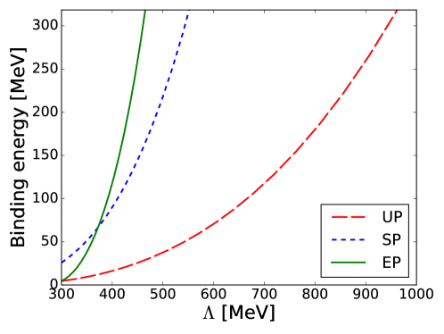
Figure 3: The ${}^{6}\mathrm{He}$ binding energy ($B=-E$) as a function of the cutoff $\Lambda$. Only the dineutron and the ${}^{5}\mathrm{He}(3/2^{-})$ channels are included. All the three-body interactions have been set to zero.

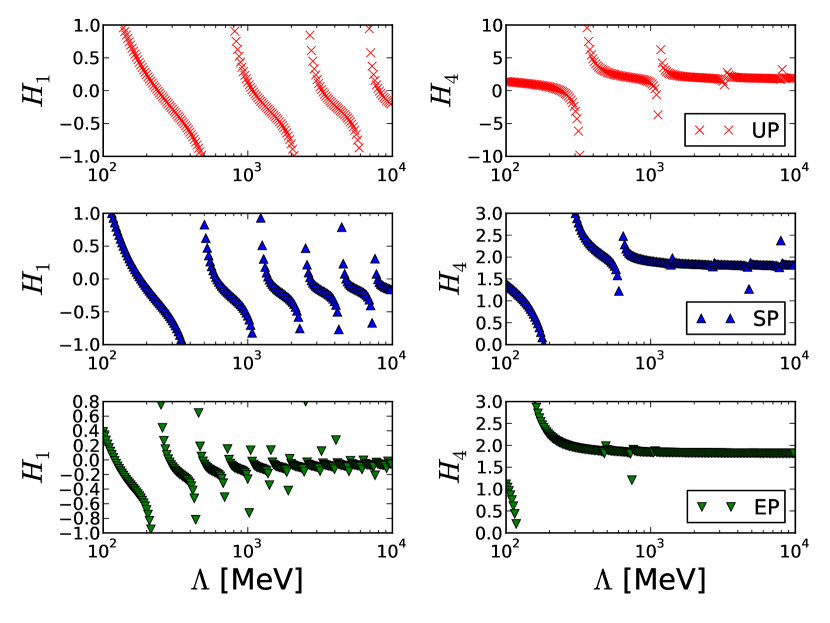
Figure 4: The running of the three-body forces $H_{1}$ (left panels) and $H_{4}$ (right panels) for the three different pole removal prescriptions. Only the dineutron and the ${}^{5}\mathrm{He}(3/2^{-})$ channels are included. The three-body parameter was fixed to reproduce the bound-state energy $E=-1~{}\mathrm{MeV}$.

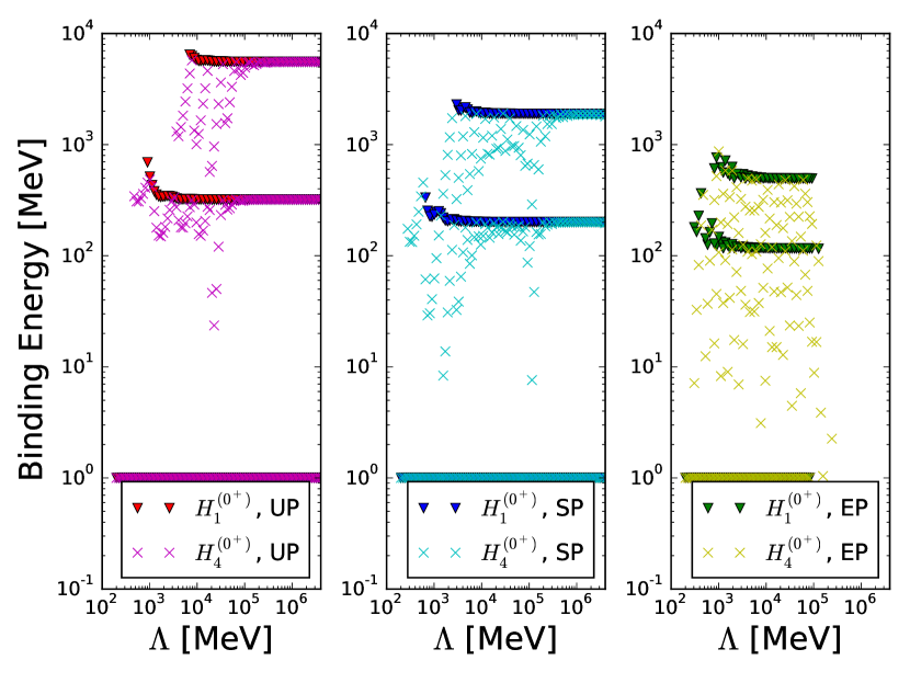
Figure 5: Convergence of deep bound states for the three different prescriptions, using either the $H_{1}$ or $H_{4}$ three-body interaction. Only the dineutron and the ${}^{5}\mathrm{He}(3/2^{-})$ channels are included. The three-body parameter was fixed to reproduce the bound-state energy $E=-1~{}\mathrm{MeV}$.

We begin by using the simpler field theory, where only the dineutron and the ${}^{5}\mathrm{He}(3/2^{-})$ channels are included. First, we set all the three-body interactions for this field theory, $H_{1}$, $H_{4}$ and $H_{5}$, to zero and evaluate the integral equations for different cutoffs. We performed these calculations using all three prescriptions (UP, SP, and EP) for the handling of the unphysical two-body poles. From this we obtain the cutoff dependence of the bound-state energy. The result of this numerical study is presented in Fig. 3. As can be seen, the bound-state energy is cutoff dependent and this implies that (at least) one three-body interaction is needed to renormalize the field theory.

We then move on to solving the integral equations for a fixed binding energy, $E=-1~{}\mathrm{MeV}$, and one varying three-body interaction. Thus, for each value of the cutoff we find the value of a selected three-body parameter that gives the fixed binding energy. For the off-diagonal three-body interaction, $H_{5}$, we did not find any solutions to the integral equation. This indicates that it can not renormalize the field theory. Using the diagonal interactions, $H_{1}$ and $H_{4}$, we generated the results, shown in Fig. 4. As before, we performed these calculations for all three unphysical-pole-removal prescriptions. It is seen that the renormalization shows a limit-cycle like behavior for both the $H_{1}$ and $H_{4}$ three-body interactions. The poles that can be seen in Fig. 4 are associated with the appearance of additional three-body bound states. The different pole removal prescriptions differ in the amount of states that are generated at larger energies since the different pole removal prescriptions lead to different large momentum behaviors in the two-body amplitude.

Finally, we also use the dineutron and ${}^{5}\mathrm{He}(3/2^{-})$ field theory to search for deep bound states in the $0^{+}$ channel. Of course, these states are not true states of ${}^{6}\mathrm{He}$, but they are still well-defined observables in the field theory. As such, if these deep bound states do not converge with increasing cutoff, then that indicates that the field theory is not properly renormalized. The procedure is as follows: First we fix either the $H_{1}$ or $H_{4}$ three-body interaction to reproduce the bound-state energy $E=-1~{}\mathrm{MeV}$ for a fixed value of the cutoff. Then, we use this three-body interaction to search for additional solutions to Eq. (39) for larger binding energies. These solutions are then deep bound states of the system. Third, we repeat the process for larger values of the cutoff. The result is then a convergence plot of these deep bound states and it is given in Fig. 5. Five findings are of particular note regarding the convergence of these deep-bound states: (i) The deep-bound states do indeed converge for large cutoffs, (ii) the convergence using the $H_{1}$ three-body interaction is much faster than using the $H_{4}$ one, (iii) the two different three-body interactions renormalize the deep bound states to the same binding energy, (iv) the three different prescriptions produce a different bound-state spectrum, and (v) using the EP we are numerically limited to cutoffs $\Lambda\lesssim 10^{5}~{}\mathrm{MeV}$ and for these cutoffs the deep bound states have not yet converged when the $H_{4}$ interaction is used. Summarizing this part, it is very encouraging that the $H_{1}$ and $H_{4}$ interactions give the same spectrum and since the $H_{1}$ produces faster convergence this motivates the use of only this three-body interaction. This conclusion is in line with previous work on the ${}^{6}\mathrm{He}(0^{+})$, where only this three-body interaction was considered, see Refs. Rotureau and van Kolck (2013); Ji et al (2014).

3.2 Field theory with dineutron, ${}^{5}\mathrm{He}(3/2^{-})$ and ${}^{5}\mathrm{He}(1/2^{-})$ channels

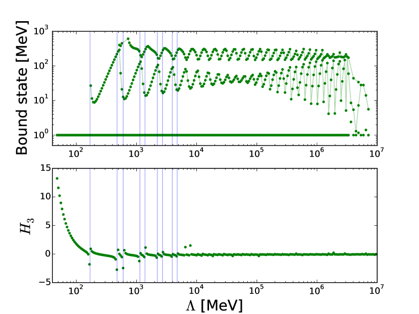
Figure 6: Non-convergence of deep bound states for a field theory where the $1/2^{-}$ channel is also included. Only the $H_{3}$ three-body interaction is used. The three-body parameter was fixed to the bound state energy $B=1~{}\mathrm{MeV}$. The vertical blue lines indicate singularities in the limit cycle and it can be seen that the oscillation of the deep bound states are given by the period of these singularities.

We now include also the ${}^{5}\mathrm{He}(1/2^{-})$ channel into the field theory. As such we have three channels to consider, which increases the computational cost by about a factor of two compared to the two-channel system. Further, there are now in total six three-body interactions at the lowest scaling dimension. However, in solving the integral equations for a bound state we did not find any solutions for the off-diagonal three-body interactions $H_{2}$, $H_{5}$ and $H_{6}$.

When a search for deep bound states was performed, using one of the diagonal three-body interactions $H_{1}$, $H_{3}$ and $H_{4}$ at a time, no convergence was observed. The cutoff dependence of the deep-bound states, using the SP and the $H_{3}$ three-body interaction, can be seen in Fig. 6. It is clear that these deep bound states are much more shallow than in the field theory without the ${}^{5}\mathrm{He}(1/2^{-})$ and we are limited to a lower cutoff, $\Lambda\lesssim 10^{6}~{}\mathrm{MeV}$. This indicates that the integral equation for the field theory with the ${}^{5}\mathrm{He}(1/2^{-})$ included is more involved numerically. The result implies that one three-body interaction is not sufficient for proper renormalization of the field theory. As such one would need to fix two, or more, three-body interactions simultaneously. However, it could also be the case that the deep bound states are renormalized at a larger cutoff than is presently accessible to us.

4 Conclusion

In this paper we have derived the LO integral equations for the treatment of the $0^{+}$ channel of ${}^{6}\mathrm{He}$ from quantum field theory. We included not only the dineutron and ${}^{5}\mathrm{He}(3/2^{-})$ channels, but also the ${}^{5}\mathrm{He}(1/2^{-})$. We analyzed all six three-body interactions that appear at the lowest mass dimension. Further, we discussed three different prescriptions of how to handle the unphysical pole in the P-wave ${}^{5}\mathrm{He}$ dicluster propagators. [[We showed that all three methods are useful but that they lead to different convergence behavior when employed in the few-body sector.]]

For a field theory where only the dineutron and the ${}^{5}\mathrm{He}(3/2^{-})$ channels were included we showed that the system was properly renormalized. In addition, both the $H_{1}$ and $H_{4}$ three-body interactions generated the same bound state spectrum. However, for a field theory where the ${}^{5}\mathrm{He}(1/2^{-})$ was also included the system was not renormalizable, at least not when only one three-body interaction was used and for cutoffs $\Lambda\lesssim 10^{6}~{}\mathrm{MeV}$.

Future studies will concern the resonant spectrum and additional total angular momentum channels, for example the ${}^{6}\mathrm{He}(2^{+})$. Our results are also relevant for future applications of Halo EFT to D-wave systems such as low-lying resonances in the Oxygen-25 and Oxygen-26 nuclei. In these systems, Oxygen-24 is interacting strongly in a relative D-wave with the neutrons. Furthermore, additional spurious poles are expected in the two-body sector due to the polynomial structure of the effective range expansion that appears after renormalization in the denominator of two-body propagators.