Effects of random potentials in three-dimensional quantum electrodynamics

Abstract

Three-dimensional quantum electrodynamics exhibits a number of interesting properties, such as dynamical chiral symmetry breaking, weak confinement, and non-Fermi liquid behavior, and also has wide applications in condensed matter physics. We study the effects of random potentials, which exist in almost all realistic condensed-matter systems, on the low-energy behaviors of massless Dirac fermions by means of renormalization group method, and show that the role of random mass is significantly enhanced by the gauge interaction, whereas random scalar and vector potentials are insusceptible to the gauge interaction at the one-loop order. The static random potential breaks the Lorentz invariance, and as such induces unusual renormalization of fermion velocity. We then consider the case in which three types of random potentials coexist in the system. The random scalar potential is found to play a dominant role in the low-energy region, and drives the system to undergo a quantum phase transition.

I Introduction

Massless three-dimensional quantum electrodynamics (QED₃) describes the interaction between massless Dirac fermions and U(1) gauge boson HeinzPRD81 ; AppelquistPRD81 ; Pisarski84 . This field theory exhibits such non-perturbative phenomena as dynamical chiral symmetry breaking (DCSB) Appelquist86 ; Appelquist88 ; Nash89 ; Atkinson90 ; Maris96 ; Fisher04 ; Bashir08 ; Lo11 ; Feng13 ; Feng14 ; Braun14 and weak confinement Burden92 ; Maris95 , and thus is often regarded as a toy model of QCD. When the fermion flavor is sufficiently large, the model is a conformal field theory Klebanov12 . QED₃ and its variants have wide applications in condensed matter physics: it is the low-energy effective theory of high-$T_{c}$ cuprate superconductors Lee06 ; Affleck ; Kim97 ; Kim99 ; Rantner ; Franz ; Herbut ; Liu02 ; Liu03 and certain spin liquid systems Ran07 ; Hermele08 ; Lu14 ; Metlitski15 ; Wang15 ; Mross15 . The non-perturbative phenomenon of DCSB provides an elegant field-theoretic description of the two-dimensional Heisenberg quantum antiferromagnetism Affleck ; Kim99 ; Franz ; Herbut ; Liu02 ; Liu03 , whereas the non-Fermi liquid behaviors induced by gauge interaction may be used to understand the observed unusual normal state of high-$T_{c}$ superconductors Lee06 ; Kim97 ; Rantner ; Franz ; Herbut ; WangLiu10A ; WangLiu10B . For these reasons, QED₃ has attracted considerable research interest in the communities of both high energy and condensed matter physics.

Previous works studying QED₃ have mainly focused on DCSB Appelquist86 ; Appelquist88 ; Nash89 ; Atkinson90 ; Maris96 ; Fisher04 ; Bashir08 ; Lo11 ; Feng13 ; Feng14 ; Braun14 and non-Fermi liquid behaviors WangLiu10A ; WangLiu10B ; WangLiu12 caused by the U(1) gauge boson in the clean limit. The effects of random potential are rarely considered in the literature. In a realistic condensed-matter system, there are always certain amount and types of random potential, which may substantially affect the dynamics of massless Dirac fermions. If some random potential is a relevant perturbation to the system, it can determine many of the low-$T$ transport properties of Dirac fermions. Moreover, random potential can also lead to instabilities of the system, which would drive various kinds of quantum phase transition. To broaden the applicability of QED₃ in condensed-matter physics, it is necessary to examine the impact of various types of random potential.

In this work, we analyze the roles played by random potentials in the low-energy region and determine all the possible infrared fixed points. To make a unbiased analysis, we shall treat the gauge interaction and random potential equally, and study their interplay by means of renormalization group (RG) method. Depending on the value of fermion flavor $N$, QED₃ stays in the DCSB phase for small $N$ and chirally symmetric phase for large $N$. Here, we suppose a large $N$ and keep Dirac fermions massless. The random potential is assumed to be static, and might be caused by defects and/or impurity atoms in various realistic condensed-matter systems. Generically, there are three types of random potential that can couple to Dirac fermions Ludwig94 ; Nersesyan95 ; Altland02 ; Stauber2005PRB ; HerbutPRL2008 ; Vafek08 ; Wang2011PRB ; WangLiu14 : random mass (RM), random scalar potential (RSP), and random vector (gauge) potential (RVP). We will first study the impact of each single random potential, and then examine how different types of random potential affect each other.

RG analysis show that the random potentials can lead to unusual renormalization of fermion velocity $v_{F}$ as a consequence of explicit Lorentz symmetry breaking. The role played by RM can be significantly enhanced by the gauge interaction, but the roles played by RVP and RSP are nearly unchanged by the gauge interaction. We also study the fixed point structure of the system with all three types of random potential present simultaneously. In this case, RSP is much more important than RM and RVP in the low-energy region, and derive the system to undergo a diffusive quantum phase transition, which occurs even when RSP is quite weak. In the absence of RSP, we find that RVP promotes the role of RM and also induce an anomalous dimension for $v_{F}$.

The rest of the paper is organized as follows. We present the whole action and the corresponding Feynman rules in Sec. II, and derive the RG equations in Sec. III. The impact of each single type of random potential and the mutual influence between different random potentials are analyzed in Sec. IV. We summarize the results and highlight possible future works in Sec. V.

II Effective action

The Lagrangian density of QED₃ with $N$ flavors of massless Dirac fermions is given by

$$\mathcal{L}_{F}=\sum_{\sigma=1}^{N}\bar{\psi}_{\sigma}\gamma^{\mu}(\partial_{\mu}+ieA_{\mu})\psi_{\sigma}-\frac{1}{4}F_{\mu\nu}^{2},$$ (1)

where $\partial_{\mu}=(\partial_{0},v_{F}\partial_{i})$ with $i=1,2$. The electromagnetic tensor is $F_{\mu\nu}=\partial_{\mu}A_{\nu}-\partial_{\nu}A_{\mu}$. Here, the Dirac fermion is described by a four-component spinor $\psi$, whose conjugate is defined as $\bar{\psi}=\psi^{{\dagger}}\gamma_{0}$. The gamma matrices can be chosen as $(\gamma_{0},\gamma_{1},\gamma_{2})=(\sigma_{3},\sigma_{2},-\sigma_{1})\otimes\sigma_{3}$, which satisfy the Clifford algebra $\{\gamma_{\mu},\gamma_{\nu}\}=2\delta_{\mu\nu}$. In (2+1) dimensions, there are two chiral matrices, denoted by $\gamma_{3}=I_{2\times 2}\otimes\sigma_{1}$ and $\gamma_{5}=-I_{2\times 2}\otimes\sigma_{2}$ respectively, which anti-commute with $\gamma_{0,1,2}$. The model contains two parameters: electric charge $e$, and fermion velocity $v_{F}$. It is easy to check that $e$ is dimensional, so this field theory is renormalizable and thus safe in the UV region. However, the gauge interaction becomes strong in the IR region, which might cause nontrivial physics.

The full theory respects the Lorentz symmetry, the U(1) local gauge symmetry, and an additional continuous $U(2N)$ chiral symmetry $\psi\rightarrow e^{i\theta\gamma_{3,5}}\psi$ with $\theta$ being an arbitrary constant if the fermions are massless. The local gauge symmetry is robust, but the other two symmetries can be easily broken, either explicitly or dynamically.

Extensive previous studies Appelquist86 ; Appelquist88 ; Nash89 ; Maris96 ; Fisher04 ; Bashir08 have confirmed that a finite fermion mass can be dynamically generated by the gauge interaction if the fermion flavor $N$ is smaller than certain critical value $N_{c}$, which leads to DCSB. In the DCSB phase, the massive fermions are confined by a logarithmic potential Burden92 ; Maris95 . For $N>N_{c}$, the Dirac fermions remain massless and thus the theory preserves the chiral symmetry. In the chirally symmetric phase, the physical properties are far from trivial as the strong gauge interaction can induce non-Fermi liquid behaviors of Dirac fermions Lee06 ; Kim97 ; Rantner ; Franz ; Herbut ; WangLiu10A ; WangLiu10B .

At zero temperature, the Lorentz invariance is strictly preserved. In this case, the fermion velocity $v_{F}$ does not renormalize at all and remains a constant. If the Lorentz invariance is broken, the gauge interaction would renormalize $v_{F}$, which then exhibits explicit dependence on momenta and energy. Thermal fluctuation definitely breaks the Lorentz invariance, and hence leads to velocity renormalization WangLiu2016 . If we stay at zero temperature but includes static random potential, the Lorentz invariance is also explicitly broken. As a result, the fermion velocity will be renormalized.

We now incorporate random potential into the Lagrangian density of QED₃ by writing down the following term Ludwig94 ; Nersesyan95 ; Altland02 ; Stauber2005PRB ; HerbutPRL2008 ; Vafek08 ; Wang2011PRB ; WangLiu14 ,

$$\mathcal{L}_{d}=\sum_{\sigma=1}^{N}\bar{\psi}_{\sigma}\left(\sum_{\Gamma}V_{\Gamma}(\mathbf{x})\Gamma\right)\psi_{\sigma},$$ (2)

where the function $V_{\Gamma}(\mathbf{x})$ stands for the randomly distributed potential. We assume $V_{\Gamma}(\mathbf{x})$ to be a quenched, Gaussian white noise potential characterized by the following identities:

$$\langle V_{\Gamma}(\mathbf{x})\rangle=0,\qquad\langle V_{\Gamma}(\mathbf{x})V_{\Gamma}(\mathbf{x}^{\prime})\rangle=\Delta_{\Gamma}\delta^{2}(\mathbf{x}-\mathbf{x}^{\prime}).$$ (3)

The random potential is classified by the expression of matrix $\Gamma$: $\Gamma=\mathbb{I}_{4\times 4}$ for RM; $\Gamma=\gamma_{0}$ for RSP; $\Gamma=(i\gamma_{1},i\gamma_{2})$ for RVP. It is also possible to include other types of random potential, but these three types are most frequently studied. The random potential can be induced by various mechanisms in realistic Dirac fermion materials Nersesyan95 ; CastroNeto ; Peres2010RMP ; Mucciolo2010JPCM ; Meyer2007Nature ; Champel2010PRB ; Kusminskiy2011PRB . These three types of random potential might exist individually, or coexist in the same material. We will first consider the impact of each single random potential, and then study their mutual influence.

The random potential $V(\mathbf{x})$ needs to be properly averaged. The simplest and most widely used scheme is to average over $V(\mathbf{x})$ by employing the replica method LeeRMP1985 ; Lerner ; Edwards1975 ; Goswami2011PRL ; LaiarXiv ; Roy2014PRB ; Roy2016PRB ; Roy2016SCP , which leads us to an effective replicated action written in the Euclidean space:

$$\overline{S} = \int d^{2}xd\tau\Big{\{}\bar{\psi}_{\sigma}^{\alpha}\left[\gamma_{0}(\partial_{0}+ieA_{0})+\gamma_{j}(v_{F}\partial_{j}+ieA_{j})\right]\psi_{\sigma}^{\alpha}$$ (4)

$$-\frac{1}{4}F_{\mu\nu}^{2}\Big{\}}-\frac{1}{2}\int d^{2}xd\tau d\tau^{\prime}\Big{[}\Delta_{M}\big{(}\bar{\psi}_{\sigma}^{\alpha}\psi_{\sigma}^{\alpha}\big{)}_{x}\big{(}\bar{\psi}_{\sigma}^{\beta}\psi_{\sigma}^{\beta}\big{)}_{x^{\prime}}$$

$$+\Delta_{S}\big{(}\bar{\psi}_{\sigma}^{\alpha}\gamma_{0}\psi_{\sigma}^{\alpha}\big{)}_{x}\big{(}\bar{\psi}_{\sigma}^{\beta}\gamma_{0}\psi_{\sigma}^{\beta}\big{)}_{x^{\prime}}+\Delta_{V}\big{(}\bar{\psi}_{\sigma}^{\alpha}i\gamma_{j}\psi_{\sigma}^{\alpha}\big{)}_{x}$$

$$\times\big{(}\bar{\psi}_{\sigma}^{\beta}i\gamma_{j}\psi_{\sigma}^{\beta}\big{)}_{x^{\prime}}\Big{]}.$$

Here, $\alpha$ and $\beta$ are the replica indices, and $x\equiv(\mathbf{x},\tau)$ and $x^{\prime}\equiv(\mathbf{x},\tau^{\prime})$. All the repeated indices are summed up automatically. To distinguish different types of random potential, we have introduced three new parameters $\Delta_{M}$, $\Delta_{S}$, and $\Delta_{V}$ to characterize the effective strength of quartic couplings of Dirac fermions induced by averaging over RM, RVP, and RSP, respectively.

We choose to work in the Euclidean space, and write the free fermion propagator as

$$G_{0}(k_{0},\mathbf{k})=\frac{-i}{\gamma_{0}k_{0}+v_{F}\bm{\gamma}\cdot\mathbf{k}}.$$ (5)

The free gauge boson propagator under Landau gauge reads

$$D^{0}_{\mu\nu}(q)=\frac{v_{F}^{2}}{Q^{2}}\left(\delta_{\mu\nu}-\frac{Q_{\mu}Q_{\nu}}{Q^{2}}\right),$$ (6)

where $Q_{\mu}\equiv(q_{0},v_{F}\mathbf{q})$ and $Q^{2}=Q_{\mu}Q_{\mu}=q_{0}^{2}+v_{F}^{2}\mathbf{q}^{2}$.

In the next section, we will perform RG calculations starting from Eq. (4). The interaction between Dirac fermions and gauge boson is treated by making a $1/N$ expansion by supposing a general large $N$. For large value of $N$, DCSB cannot take place and the Dirac fermions are kept massless throughout our calculations. However, the parameters $\Delta_{M}$, $\Delta_{S}$, and $\Delta_{V}$ are assumed to be small, corresponding to the nearly clean case.

III Derivation of RG equations

In this section, we calculate the quantum corrections to the polarization tensor, fermion self-energy, fermion-disorder vertex, and gauge coupling vertex to the leading order of perturbative expansion. Based on these results, we will be able to derive the RG flow equations for all the free model parameters.

III.1 Polarization tensor and fermion self-energy

At the one-loop level, the diagram for the polarization function are shown in Fig. 1. It is straightforward to get

$$\Pi_{\mu\nu}(q) = Ne^{2}\int\frac{d^{3}k}{(2\pi)^{3}}\mathrm{Tr}\left[G(k)\gamma_{\mu}G(k+q)\gamma_{\nu}\right],$$ (7)

$$= Ne^{2}\frac{1}{v_{F}^{2}}\int\frac{d^{3}K}{(2\pi)^{3}}\mathrm{Tr}\left[G(K)\gamma_{\mu}G(K+Q)\gamma_{\nu}\right],$$

$$= \Pi(Q)\left(\delta_{\mu\nu}-\frac{Q_{\mu}Q_{\nu}}{Q^{2}}\right),$$

where the function

$$\Pi(Q)=-\frac{\alpha Q}{v_{F}^{2}}$$ (8)

with $\alpha=Ne^{2}/8$. For massless QED₃, the dimensional coupling $\alpha=Ne^{2}/8$ is kept fixed as $N\rightarrow\infty$, providing the only fixed energy scale in the theory AppelquistPRD81 ; HeinzPRD81 ; Pisarski84 ; Appelquist86 ; Appelquist88 ; Nash89 . Including the corrections to the polarization function, we write the effective gauge boson propagator in the form

$$D_{\mu\nu}(Q) = \frac{v_{F}^{2}}{Q^{2}+\alpha Q}\left(\delta_{\mu\nu}-\frac{Q_{\mu}Q_{\nu}}{Q^{2}}\right)$$ (9)

$$\approx \frac{v_{F}^{2}}{\alpha Q}\left(\delta_{\mu\nu}-\frac{Q_{\mu}Q_{\nu}}{Q^{2}}\right).$$

The quantum corrections is rapidly damped for momenta $Q>\alpha$ Appelquist88 ; Nash89 ; Maris96 , thus the above approximation is well justified and also has been widely used Kim97 ; Kim99 ; Franz .

Diagrams for fermion self-energy are shown in Fig. 2. According to Fig. 2, the correction due to gauge interaction to the leading order of $1/N$ expansion is

$$\Sigma^{G}(p_{0},\mathbf{p}) = -e^{2}\int\frac{d^{3}q}{(2\pi)^{3}}\gamma_{\mu}G(p-q)\gamma_{\nu}D_{\mu\nu}(Q)$$ (10)

$$= i\eta_{\psi}\gamma_{\mu}P_{\mu}\ln b.$$

Here, the momenta integration is restricted within the shell $Q\in[\Lambda/b,\Lambda]$, where $\Lambda$ is an UV cutoff and $b=e^{l}$ with $l\geq$ being a freely varying length scale. We use $\eta_{\psi}$ to denote the anomalous dimension of the fermion wave function renormalization. To the leading order, we have

$$\eta_{\psi}=\frac{8}{3\pi^{2}N},$$ (11)

which is in accordance with Refs. Atkinson90 ; Maris96 .

Figure 1: One-loop Feynman diagram for polarization tensor, where solid line stands for the free fermion propagator and wavy line for the bare gauge boson propagator.

Figure 2: One-loop fermion self-energy due to (a) gauge interaction; (b) random potential (dashed line).

Form the above calculations, we can see that the fermion velocity $v_{F}$ is not renormalized at all, which means $v_{F}$ is a constant independent of varying energy scale. It is therefore safe to set $v_{F}\equiv 1$ and recover $v_{F}$ whenever necessary. However, when static random potential is added to the system, the Lorentz symmetry is explicitly broken, and $v_{F}$ may received singular corrections.

According to Fig. 2, the one-loop disorder-induced fermion self-energy is given by

$$\Sigma_{\mathrm{dis}}(k_{0}) = \sum_{\Gamma}\Delta_{\Gamma}\int\frac{d^{2}\mathbf{k}}{(2\pi)^{2}}\Gamma G_{0}(k_{0},\mathbf{k})\Gamma$$ (12)

$$= -ik_{0}\sum_{\Gamma}\frac{\Delta_{\Gamma}\Gamma\gamma_{0}\Gamma}{2\pi v_{F}^{2}}\ln b$$

$$= -ik_{0}\gamma_{0}\frac{\Delta_{S}+\Delta_{M}+2\Delta_{V}}{2\pi v_{F}^{2}}\ln b.$$

It is clear that random potential does not lead to wave function renormalization of spatial components, so $v_{F}$ will be renormalized.

III.2 Gauge coupling and fermion-disorder vertex

Besides the gauge coupling parameter, disorder also bring another kind of parameter which is the effective strength of coupling between fermion and disorder. At this subsection, these vertices corrections are computed.

The one-loop diagrams gauge coupling corrections are depicted in Fig. 3. At vanishing external momenta and energy, the vertex correction due to gauge interaction shown in Fig. 3 is

$$V_{\mathrm{e}}^{G} = -ie^{3}\int\frac{d^{3}q}{(2\pi)^{3}}\gamma_{\rho}G_{0}(q)\gamma_{\mu}G_{0}(q)\gamma_{\nu}D_{\rho\nu}(Q)$$ (13)

$$= -ie\gamma_{\mu}\eta_{\psi}\ln b.$$

According to Fig. 3, the gauge coupling correction due to random potential at zero external momenta-energy is

$$V_{\mathrm{e}}^{d} = ie\sum_{\Gamma}\Delta_{\Gamma}\int\frac{d^{2}\mathbf{k}}{(2\pi)^{2}}\Gamma G_{0}(k_{0},\mathbf{k})\gamma_{\mu}G_{0}(k_{0},\mathbf{k})\Gamma$$ (14)

$$= ie\gamma_{0}\frac{\Delta_{S}+\Delta_{M}+2\Delta_{V}}{2\pi v_{F}^{2}}\ln b.$$

In the replica limit, the one loop Feynman diagrams for the corrections to fermion-disorder vertex are shown in Fig. 4. At zero external momentum and frequency, the corresponding correction induced by gauge interaction depicted in Fig. 4(a) is calculated as

$$V_{\mathrm{dis}}^{G} = e^{2}\Delta_{\Gamma}\int\frac{d^{3}q}{(2\pi)^{3}}\gamma_{\mu}G_{0}(q)\Gamma G_{0}(q)\gamma_{\nu}D_{\mu\nu}(Q)$$ (15)

$$= a\eta_{\psi}\ln b(\Delta_{\Gamma}\Gamma),$$

where $a=-3$ for RM, and $a=1$ for RSP and RVP. Fig. 4(b) is the vertex correction due to disorder averaging, and given by

$$V_{\mathrm{dis}}^{d} = \Delta_{a}\sum_{\Gamma_{b}}\Delta_{b}\int\frac{d^{2}\mathbf{q}}{(2\pi)^{2}}\Gamma_{b}G_{0}(q_{0},\mathbf{q})\Gamma_{a}G_{0}(q_{0},\mathbf{q})\Gamma_{b},$$

After analytical calculations, we get

$$V_{\mathrm{dis}}^{d} = \frac{-(\Delta_{S}+\Delta_{M}+2\Delta_{V})\Delta_{M}}{2\pi v_{F}^{2}}\mathbb{I}_{4\times 4}\ln b$$ (17)

for RM,

$$V_{\mathrm{dis}}^{d} = \frac{(\Delta_{S}+\Delta_{M}-2\Delta_{V})\Delta_{S}}{2\pi v_{F}^{2}}\gamma_{0}\ln b,$$ (18)

for RSP, and

$$V_{\mathrm{dis}}^{d} = 0.$$ (19)

for RVP. The sum of the two diagrams given by Fig. 4(c) and Fig. 4(d) produces a nonzero correction to another type of random potential defined by the matrix $\Gamma=\gamma_{0}\bm{\gamma}$ along with parameters $(\Gamma_{a},\Gamma_{b})=(\mathbb{I}_{4\times 4},\gamma_{0})$ Goswami2011PRL ; Roy2016SCP . However, this type of random potential is not considered in the present paper. For the three types of random potential under consideration, the contributions from Fig. 4(c) and Fig. 4(d) simply cancel each other by virtue of the relation Roy2014PRB ; LaiarXiv : $G(-k_{0},-\mathbf{k})=-G(k_{0},\mathbf{k})$.

Figure 3: One-loop gauge coupling correction due to (a) gauge interaction, (b) random potential.

Figure 4: One-loop corrections to the coupling vertex between fermions and random potentials in the vanishing replica limit.

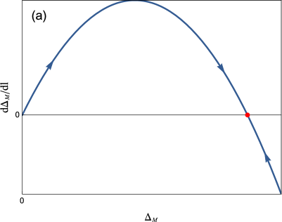
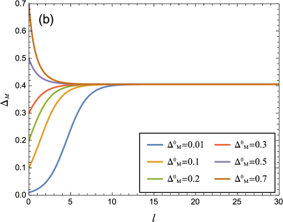
Figure 5: (a) Flow diagram of $\Delta_{M}$ for RM. There is an unstable Gaussian fixed point $\Delta_{M}=0$ and a finite stable fixed point $\Delta_{M}=4\eta_{\psi}+2\Delta_{V}^{0}$. (b) Dependence of $\Delta_{M}$ on the running scale $l$ at different initial values. Here, $N=4$ and $\Delta_{V}^{0}=0.07$.

III.3 RG equations for model parameters

To perform RG analysis, we rescale the frequency and momenta as follows Shankar94

$$\tilde{x}_{\mu}=x_{\mu}b^{-1}.$$ (20)

The field operators and model parameters are rescaled in the following way

$$\tilde{\psi}=\sqrt{Z_{\psi}}\psi,\,\,\,\,\tilde{\Delta}_{\Gamma}=\sqrt{Z_{\Gamma}}\Delta_{\Gamma},$$

$$\tilde{v}_{F}=Z_{v}v_{F},\,\,\,\,\tilde{e}=Z_{e}e.$$ (21)

On the basis of the above scaling transformations, we obtain the complete set of RG equations:

$$\frac{de^{2}}{d\ln b} = e^{2}-\frac{N}{8}e^{4},$$ (22)

$$\frac{d\Delta_{M}}{d\ln b} = -2\Delta_{M}(\Delta_{M}+\Delta_{S}-2\Delta_{V}-4\eta_{\psi}),$$ (23)

$$\frac{d\Delta_{S}}{d\ln b} = 2\Delta_{S}(\Delta_{M}+\Delta_{S}+2\Delta_{V}),$$ (24)

$$\frac{d\Delta_{V}}{d\ln b} = 0,$$ (25)

$$\frac{dv_{F}}{d\ln b} = -(\Delta_{M}+\Delta_{S}+2\Delta_{V})v_{F}.$$ (26)

In the derivation of RG equations, we have redefined the renormalized gauge coupling as Kubota2001 ; Gusynin2001PRD

$$e^{2}(p)=\frac{e^{2}}{1-\Pi(p)},$$ (27)

which naturally gives rise to the flow Eq. (22). Moreover, the effective parameter for random potentials are redefined as

$$\Delta_{\Gamma}/(2\pi v_{F}^{2})\rightarrow\Delta_{\Gamma}.$$ (28)

Eq. (22) shows that the flow equation of gauge coupling is not affected by random potentials at the leading order. This reflects the fact that random potential does not couple directly to the gauge boson. Their mutual effects can only be induced by their separate interaction with Dirac fermions, which are higher order corrections to the leading order results. Indeed, the flow equation Eq. (22) coincides with previous results JanssenarXiv ; KavehPRB2005 ; HerbutPRD2016 and exhibits a stable infrared fixed point at $e_{\ast}^{2}\sim O(1/N)$ to the leading order of perturbative expansion. The rest four RG equations, i.e., Eqs. (23) - (25) incorporate the influence of random potentials, and are apparently absent in the clean limit with $\Delta_{M}=\Delta_{S}=\Delta_{V}=0$.

According to Eqs. (23) - (25), we observe that RM is the only random potential that is directly influenced by the gauge interaction. For RSP, the flow of $\Delta_{S}$ depends sensitively on the interplay of different random potentials. The effective parameter for RVP, namely $\Delta_{V}$, simply does not flow with varying energy scale, which is a consequence of the existence of a time-independent gauge transformation that ensures RVP unrenormalized and is valid at any order of loop expansion HerbutPRL2008 . Some previous works HerbutPRL2008 ; Vafek08 have studied the RG flow of $\Delta_{V}$ by considering the interplay of long-range Coulomb interaction and RVP in graphene. It was found HerbutPRL2008 ; Vafek08 that the parameter $\Delta_{V}$ also does not flow.

IV Interplay between gauge interaction and random potentials

In this section, we analyze the RG solutions and also discuss the physical effects of random potential on Dirac fermions. Since $\Delta_{V}$ does not flow, it can be taken at certain constant. We will always retain gauge interaction and RVP with $\Delta_{V}=\Delta_{V}^{0}$ in the system, and study how the system is influenced by RM and by RSP, respectively. We then consider the most general case in which the gauge interaction and all three types of random potentials coexist in the system. Our aim is to find out the possible infrared fixed points, which will be used to judge the relevance (or irrelevance) of random potential.

IV.1 Random mass

In the case of RM, we set $\Delta_{S}=0$ and $\Delta_{V}=\Delta_{V}^{0}$, which simplify the RG equations of $\Delta_{M}$ and $v_{F}$ to

$$\frac{d\Delta_{M}}{dl} = -2\Delta_{M}(\Delta_{M}-2\Delta_{V}^{0}-4\eta_{\psi}),$$ (29)

$$\frac{dv_{F}}{dl} = -(\Delta_{M}+2\Delta_{V}^{0})v_{F},$$ (30)

where $\eta_{\psi}$ is the anomalous dimension induced by gauge interaction and $\Delta_{V}^{0}$ is a small constant. The solution for Eq. (29) has the following form

$$\Delta_{M}(l)=\frac{2\Delta_{M}^{0}(2\eta_{\psi}+\Delta_{V}^{0})e^{4(2\eta_{\psi}+\Delta_{V}^{0})l}}{\Delta_{M}^{0}[e^{4(2\eta_{\psi}+\Delta_{V}^{0})l}-1]+2(2\eta_{\psi}+\Delta_{V}^{0})},$$ (31)

where $\Delta_{M}^{0}$ is the value of $\Delta_{M}$ defined at the UV cutoff. It is easy to find that

$$\lim_{l\rightarrow\infty}\Delta_{M}(l)=2(2\eta_{\psi}+\Delta_{V}^{0}).$$ (32)

in the long wavelength limit, which clearly tells us that $\Delta_{M}^{\ast}=2(2\eta_{\psi}+\Delta_{V}^{0})$ is the only stable infrared fixed point. In addition, one can verify that $\Delta_{M}$ also has an unstable Gaussian fixed point $\Delta_{M}^{\ast}=0$. The existence of these two fixed points is illustrated in Figs. 5-5. According to Eq. (32), the finite stable infrared point can be produced by both the gauge interaction and RVP. Therefore, as along as RM coexists with one of this two kinds of interaction, it will becomes a marginally relevant perturbation to the system.

To gain a better understanding of the impact of gauge interaction and RVP on RM, it is interesting to take a look at the coupling between RM and fermions. When the system contains only RM and Dirac fermions, RG analysis show that $\Delta_{M}^{\ast}=0$ is the only stable fixed point. Although RM is marginally irrelevant in the absence of gauge interaction and RVP, its importance can be significantly enhanced by the gauge interaction and RVP. We know from the above discussion that RM becomes marginally relevant when it coexists with with the gauge interaction. Such an interaction-induced enhancement of random potential appears to be a generic property of several planar strongly correlated systems ZhaoPRB2016 ; Stauber2005PRB ; Goswami2011PRL . Reminding that we are employing a weak coupling expansion for the coupling between fermions and random potential. The infrared stable fixed point generated by gauge interaction is at the order of $O(1/N)$, thus the weak coupling expansion in the case of RM is reliable. Moreover, when RM and RVP coexist in the system without gauge interaction, the finite fixed point is still present. Therefore, RVP can also enhance RM OstrovskyPRB2006 ; FosterPRB2012 .

The enhancement of the role of RM by gauge interaction can be made clearer by analyzing the low-energy behaviors of fermion velocity $v_{F}$. Substituting Eq. (31) into Eq. (30), and then solving the differential equations, we obtain

$$v_{F}(l)=\frac{v_{F}^{0}e^{-2\Delta_{V}^{0}l}}{\sqrt{t_{m}[e^{4(2\eta_{\psi}+\Delta_{V}^{0})l}-1]+1}},$$ (33)

where

$$t_{m}\equiv\Delta_{M}^{0}/2(2\eta_{\psi}+\Delta_{V}^{0})$$ (34)

and $v_{F}^{0}$ is the initial value of $v_{F}$ at upper cutoff $\Lambda$. We first consider the simplest case in which Dirac fermions couple to RM alone. Since $\eta_{\psi}=\Delta_{V}^{0}=0$, the function $v_{F}(l)$ becomes

$$v_{F}(l)=\frac{v_{F}^{0}}{\sqrt{2\Delta_{M}^{0}l+1}}.$$ (35)

Thus, $v_{F}(l)$ is driven by RM to decrease with growing $l$ grows and vanishes as $l\rightarrow+\infty$. However, this is not a exponential decay for which there is no anomalous dimension generated for $v_{F}$. Indeed, RM only generates a logarithmic correction to $v_{F}$.

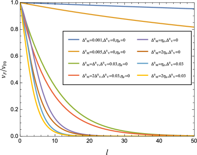
Figure 6: Dependence of $v_{F}(l)$ on the running scale $l$ at different initial values of $\Delta_{M},\Delta_{V}$. Here, $\eta_{\psi}=0$ represents the case without gauge interaction. For nonzero $\eta_{\psi}$, we assume $N=4$.

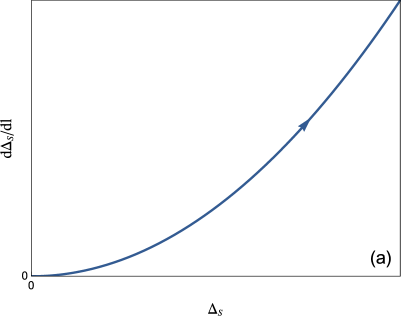
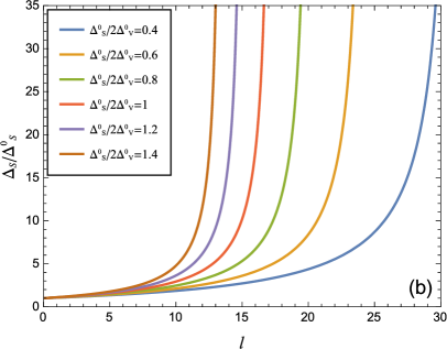
Figure 7: (a) Flow diagram of $\Delta_{S}$ for RSP. There is only a unstable Gaussian fixed point $\Delta_{S}=0$. (b) Dependence of $\Delta_{S}$ on the running scale $l$ at different initial values of $\Delta_{S}/2\Delta_{V}^{0}$. Here, $\Delta_{V}^{0}=0.01$.

We now add the gauge interaction into the system but keep $\Delta_{V}^{0}=0$, and find that Eq. (33) becomes

$$v_{F}(l)=\frac{v_{F}^{0}}{\sqrt{t_{m}^{G}(e^{8\eta_{\psi}l}-1)+1}},$$ (36)

where $t_{m}^{G}\equiv\Delta_{M}^{0}/4\eta_{\psi}$. In the lowest-energy limit, the velocity behaves as

$$v_{F}(l)\big{|}_{l\rightarrow\infty}\sim v_{F}^{0}/\sqrt{t_{m}^{G}}e^{-4\eta_{\psi}l}.$$ (37)

In this case, $v_{F}(l)$ flows to zero exponentially with growing $l$. The function Eq. (37) can be re-expressed as a function of momentum $k$ in the form

$$v_{F}(k)\propto k^{\eta_{v}},$$ (38)

where $\eta_{v}=4\eta_{\psi}=32/3\pi^{2}N$ corresponds to the stable infrared fixed point of RM produced by the gauge interaction. We can see that $v_{F}$ now acquires a finite anomalous dimension $\eta_{v}$, which takes a universal constant at a given flavor $N$. The expression of this anomalous dimension is analogous to that obtained in Ref. WangLiu12 which studied the fermion velocity renormalization in QED₃ defined at finite fermion density. Moreover, this kind of fermion velocity renormalization is a special property of Dirac fermion systems, including graphene Vafek07 ; Son07 ; WangLiuNJP12 ; WangLiu14 ; Kotov and high-$T_{c}$ superconductors Kim97 ; Xu08 ; Huh08 ; Liu12 ; She15 . It leads to a series of extraordinary spectral, thermodynamic, and transport properties of massless Dirac fermions Vafek07 ; Son07 ; WangLiuNJP12 ; WangLiu14 ; Kotov ; Kim97 ; Xu08 ; Huh08 ; Liu12 ; She15 .

We then remove the gauge boson and consider the coexistence of RVP and RM. In this case, Eq. (33) becomes

$$v_{F}(l)=\frac{v_{F}^{0}e^{-2\Delta_{V}^{0}l}}{\sqrt{t_{m}^{d}(e^{4\Delta_{V}^{0}l}-1)+1}},$$ (39)

where $t_{m}^{d}\equiv\Delta_{M}^{0}/2\Delta_{V}^{0}$. It is easy to find that the velocity varies with $l$ as

$$v_{F}(l)\big{|}_{l\rightarrow\infty}\sim v_{F}^{0}/\sqrt{t_{m}^{d}}e^{-4\Delta_{V}^{0}l},$$ (40)

Similarly, $v_{F}(l)$ flows to zero exponentially as $l$ grows. We then convert Eq. (40) to the expression

$$v_{F}(k)\propto k^{\eta_{v}}.$$ (41)

with $\eta_{v}=4\Delta_{V}^{0}$ corresponds to the stable infrared fixed point induced by RVP and RM. It is thus clear that, similar to the gauge interaction, RVP can also enhance role played by RM and induce an anomalous dimension of $v_{F}$ that is proportional to the strength of RVP.

When RM coexists with both the gauge interaction and RVP, the fermion velocity acquires an anomalous dimension $\eta_{v}=2(2\eta_{\psi}+\Delta_{V}^{0})$. We present the detailed $l$-dependence of $v_{F}$ in Fig. 6 for the four different cases discussed in this subsection.

IV.2 Random scalar potential

We then remove RM and add RSP to the system. By setting $\Delta_{M}=0$ and $\Delta_{V}=\Delta_{V}^{0}$, we get the RG equations of $\Delta_{S}$ and $v_{F}$ in the presence of RSP:

$$\frac{d\Delta_{S}}{dl} = 2\Delta_{S}(\Delta_{S}+2\Delta_{V}^{0}),$$ (42)

$$\frac{dv_{F}}{dl} = -(\Delta_{S}+2\Delta_{V}^{0})v_{F}.$$ (43)

The corresponding flow diagram is schematically shown in Fig. 7-7. We find that there is only one unstable Gaussian fixed point $\Delta_{S}^{\ast}=0$. As $l$ increases, $\Delta_{S}(l)$ exhibits a run-away behavior for any small initial value. To illustrate this fact more quantitatively, we obtain the following solution:

$$\Delta_{S}(l)=\frac{2\Delta_{S}^{0}\Delta_{V}^{0}}{(\Delta_{S}^{0}+2\Delta_{V}^{0})e^{-4\Delta_{V}^{0}l}-\Delta_{S}^{0}}.$$ (44)

Therefore, the renormalized parameter $\Delta_{S}$ increases rapidly with growing $l$ and formally diverges at a finite length scale $l_{c}=1/4\Delta_{V}^{0}\ln\left[1+2\Delta_{V}^{0}/\Delta_{S}^{0}\right]$. However, we should emphasize that $\Delta_{S}$ does not really diverge. The superficial runaway behavior of $\Delta_{S}$ triggers an instability of the Dirac fermion system, which undergoes a quantum phase transition that drives the Dirac fermions to move diffusively Fradkin1986 ; Shindou2009 ; Goswami2011PRL ; Roy2014PRB ; Syzranov2015 ; Kobayashi2014 ; Biswas2014 . The Dirac fermions acquire a finite scattering rate $\gamma_{\mathrm{im}}$ in the diffusive phase, and damp with time in the form Liliu2010

$$G(t)\propto e^{-i\gamma_{\mathrm{im}}t}.$$

It is interesting that such a diffusive transition occurs even if RSP is arbitrarily weak. According to Eq. (42), we find that this diffusive behavior already exists when there is only RM in a Dirac fermion system. It turns out that adding RVP to the system promotes the role of RM and catalyzes the diffusive transition.

The rapid increase of $\Delta_{S}$ drives $v_{F}$ to vanish at the length scale $l_{c}$. To show this, we substitute Eq. (44) into Eq. (43), and then get a solution

$$v_{F}(l)=v_{F}^{0}\sqrt{-t_{s}+e^{-4\Delta_{V}^{0}l}(t_{s}+1)},$$ (45)

where $t_{s}\equiv\Delta_{S}^{0}/2\Delta_{V}^{0}$. It is easy to verify that

$$v_{F}(l)\big{|}_{l\rightarrow l_{c}}=0,$$ (46)

which can also be observed from Fig. 8. However, it is necessary to emphasize that this limiting behavior is only artificial. The expression of $v_{F}(l)$ is indeed unreliable because the perturbative RG method breaks down before $l$ approaches $l_{c}$. To obtain a reliable expression for $v_{F}$ in the low-energy regime, one should carefully study the diffusive phase Roy2014PRB ; Moon2014arXiv , which is very interesting but beyond the scope of the present work.

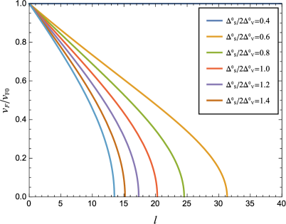
Figure 8: Dependence of $v_{F}(l)$ on the running scale $l$ at different initial values of $\Delta_{S}/2\Delta_{V}^{0}$. Here, $\Delta_{V}^{0}=0.01$.

IV.3 Random vector potential

There exists a peculiar time-independent gauge transformation in the presence of RVP HerbutPRL2008 ; Vafek08 , which renders that the parameter of RVP is unrenormalized and insusceptible to the gauge interaction and the rest two types of random potential. Due to this property, $\Delta_{V}$ can be regarded as a constant. Now Eq. (26) is simplified to

$$\frac{dv_{F}}{dl}=-2\Delta_{V}^{0}v_{F},$$ (47)

which has a solution

$$v_{F}(l)=v_{F}^{0}e^{-2\Delta_{V}^{0}l},$$ (48)

The velocity depends on $k$ as follows

$$v_{F}(k)\propto k^{\eta_{v}},$$ (49)

with $\eta_{v}=2\Delta_{V}^{0}$.

It is clear that RVP alone is able to induce unusual fermion velocity renormalization with an anomalous dimension $\eta_{v}=2\Delta_{V}^{0}$. In particular, the velocity $v_{F}$ is strongly suppressed by RVP at low energies, which in turn increases the effective strength of RM and RSP, as can be seen from Eq. (28).

IV.4 Interplay between RM and RSP

We have thus far only considered how RM and RSP are separately affected by the gauge interaction and RVP. We finally consider the general case in which both RM and RSP exist in the system, and study their mutual influence. The flow equations for $\Delta_{M}$ and $\Delta_{M}$ can be written as follows

$$\frac{d\Delta_{M}}{d\ln b} = -2\Delta_{M}(\Delta_{M}+\Delta_{S}-2\Delta_{V}-4\eta_{\psi}),$$ (50)

$$\frac{d\Delta_{S}}{d\ln b} = 2\Delta_{S}(\Delta_{M}+\Delta_{S}+2\Delta_{V}).$$ (51)

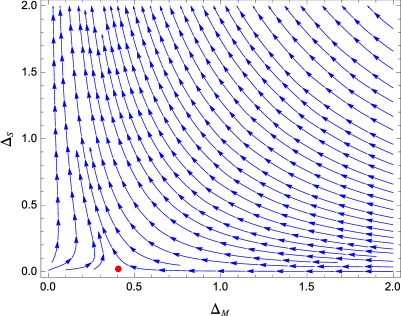
Figure 9: Schematic flow diagram in the plane spanned by $\Delta_{M}$ and $\Delta_{S}$, where $N=4$ and $\Delta_{V}^{0}=0.07$.

The analytical solution of these equations are hard to obtain. We solve them numerically and present the schematic RG flow diagram in Fig. 9. One interesting result is that the stable infrared fixed point obtained in Sec. IV.1 in the case of RM is eliminated by the coexisting RSP, irrespective of the strength of RSP. Actually, RM flows to the trivial Gaussian fixed point as along as RSP is present. It can be concluded that RM is entirely suppressed by RSP even when the system also contains the gauge interaction and RVP. Similar to the case without RM, RSP still shows a run-away behavior and drives a diffusive phase transition. It turns out that RSP plays a dominant role at low energies and determines most of the low-energy properties of the system, with RM and RVP being nearly negligible.

V Summary and discussion

In summary, we have studied the effects of three types of random potential on the low-energy behaviors of Dirac fermions in the context of QED₃. After carrying out RG calculations, we have showed that RM, RSP, and RVP can substantially affect the properties of mass Dirac fermions. Adding random potentials to the system explicitly breaks the Lorentz invariance, and leads to fermion velocity renormalization. We have computed the renormalized velocity and analyzed its low-energy asymptotic behaviors. The role played by RM is significantly enhanced by the gauge interaction but RSP and RVP seems to be insusceptible to the gauge interaction at the one-loop order. RSP is a marginally relevant perturbation to the system, and drives the system to undergo a diffusive quantum phase transition. When three types of random potentials coexist, RSP dominates and determines the low-energy behavior of the system, with RM and RVP being nearly ignorable. In the absence of RSP, RVP promotes RM to become a marginally relevant perturbation, and also induces an anomalous dimension for fermion velocity.

After determining the infrared fixed point structure of QED₃ with random potentials, the next task could be to analyze the low-energy behaviors induced by the unusual renormalization of fermion velocity. It is also interesting to study the rich quantum critical phenomena at the diffusive quantum critical point, and compute the associated critical exponents and observable quantities Goswami2011PRL ; Roy2014PRB ; Roy2016PRB ; LaiarXiv ; Syzranov2015 ; Pixley2016 ; Syzranov2016 ; Isobe2016PRL .

In the condensed-matter applications, QED₃ may need to be properly modified. For example, in the effective QED₃ theory of high-$T_{c}$ superconductors Lee06 ; Kim97 , the gauge boson couples to massless Dirac fermions and additional scalar bosons. It would be straightforward to include these additional degrees of freedom into the RG analysis performed in this work.

Note added.—After the original version of this paper was submitted out for publication, we became aware of two related works by Goswami, et al. Goswami17 and by Thomson and Sachdev Thomson17 , who have studied the effects of some sorts of quench disorder in QED₃. For the three sorts of disorder considered in our paper, our RG equations are in accordance with those of Ref.Thomson17 . In particular, the same fixed-point structure for the strength parameters of gauge interaction and disorder was obtained in both of our works. Moreover, these three works all have reached a common conclusion for RMP that there exists a finite fixed point in the space spanned by the parameters for gauge interaction and disorder. In the case of RSP, however, the results obtained in our work and in Ref.Thomson17 are quite different from Ref.Goswami17 , where it is claimed that RSP is screened and that the fixed point for gauge interaction is stable against RSP. This difference stems from the fact that both our work and Ref.Thomson17 ignore the Feynman diagrams presented in Fig.1 of Ref.Goswami17 , which are free of divergence and thus should not be incorporated in the RG analysis performed in exactly three space-time dimensions. Moreover, in this paper we have made a detailed analysis of the interplay between different types of disorder, which have not been considered in Ref.Goswami17 and Ref.Thomson17 .

References

- (1) T. Appelquist and U. Heinz, Phys. Rev. D 24, 2169 (1981).
- (2) T. Appelquist and R. Pisarski, Phys. Rev. D 21, 2305 (1981).
- (3) R. D. Pisarski, Phys. Rev. D 29, 2423(R) (1984).
- (4) T. W. Appelquist, M. Bowick, D. Karabali, and L. C. R. Wijewardhana, Phys. Rev. D 33, 3704 (1986).
- (5) T. Appelquist, D. Nash, and L. C. R. Wijewardhana, Phys. Rev. Lett. 60, 2575 (1988).
- (6) D. Nash, Phys. Rev. Lett. 62, 3024 (1989).
- (7) P. Maris, Phys. Rev. D 54, 4049 (1996).
- (8) D. Atkinson, P. W. Johnson, and P. Maris, Phys. Rev. D 42, 602 (1990).
- (9) C. S. Fischer, R. Alkofer, T. Dahm, and P. Maris, Phys. Rev. D 70, 073007 (2004).
- (10) A. Bashir, A. Raya, I. C. Cloët, and C. D. Roberts, Phys. Rev. C 78, 055201 (2008).
- (11) P. M. Lo and E. S. Swanson, Phys. Rev. D 83, 065006 (2011).
- (12) H.-T. Feng, Y.-Q. Zhou, P.-L. Yin, and H.-S. Zong, Phys. Rev. D 88, 125022 (2013).
- (13) H.-T. Feng, J.-F. Li, Y.-M. Shi, and H.-S. Zong, Phys. Rev. D 90, 065005 (2014).
- (14) J. Braun, H. Gies, L. Janssen, and D. Roscher, Phys. Rev. D 90, 036002 (2014).
- (15) C. J. Burden, J. Praschifka, and C. D. Roberts, Phys. Rev. D 46, 2695 (1992).
- (16) P. Maris, Phys. Rev. D 52, 6087 (1995).
- (17) I. R. Klebanov, S. S. Pufu, S. Sachdev, and B. R. Safdi, J. High Energy Phys. 5, 036 (2012).
- (18) I. Affleck and J. B. Marston, Phys. Rev. B 37, 3774 (R) (1988); L. B. Ioffe and A. I. Larkin, Phys. Rev. B 39, 8988 (1989).
- (19) D. H. Kim and P. A. Lee, Ann. Phys. (NY) 272, 130 (1999).
- (20) G.-Z. Liu and G. Cheng, Phys. Rev. B 66, 100505(R) (2002).
- (21) G.-Z. Liu and G. Cheng, Phys. Rev. D 67, 065010 (2003).
- (22) M. Franz and Z. Teanovi, Phys. Rev. Lett. 87, 257003 (2001); M. Franz, Z. Teanovi, and O. Vafek, Phys. Rev. B 66, 054535 (2002).
- (23) I. F. Herbut, Phys. Rev. Lett. 88, 047006 (2002); Phys. Rev. B 66, 094504 (2002).
- (24) P. A. Lee, N. Nagaosa, and X.-G. Wen, Rev. Mod. Phys. 78, 17 (2006).
- (25) D. H. Kim, P. A. Lee, and X.-G. Wen, Phys. Rev. Lett. 79, 2109 (1997).
- (26) W. Rantner and X.-G. Wen, Phys. Rev. Lett. 86, 3871 (2001); Phys. Rev. B 66, 144501 (2002).
- (27) Y. Ran, M. Hermele, P. A. Lee, and X.-G. Wen, Phys. Rev. Lett. 98, 117205 (2007).
- (28) M. Hermele, Y. Ran, P. A. Lee, and X.-G. Wen, Phys. Rev. B 77, 224413 (2008).
- (29) Y.-M. Lu and D.-H. Lee. Phys. Rev. B 89, 195143 (2014).
- (30) M. A. Metlitski and A. Vishwanath, Phys. Rev. B 93, 245151 (2016).
- (31) C. Wang and T. Senthil, Phys. Rev. X 5, 041031 (2015).
- (32) D. F. Mross, J. Alicea, and O. Motrunich, Phys. Rev. Lett. 117, 016802 (2016).
- (33) J.-R. Wang and G.-Z. Liu, Nucl. Phys. B 832, 441 (2010).
- (34) J.-R. Wang and G.-Z. Liu, Phys. Rev. B 82, 075133 (2010).
- (35) J. Wang and G.-Z. Liu, Phys. Rev. D 85, 105010 (2012).
- (36) A. W. W. Ludwig, M. P. A. Fisher, R. Shankar, and G. Grinstein, Phys. Rev. B 50, 7526 (1994).
- (37) A. A. Nersesyan, A. M. Tsvelik, and F. Wenger, Nucl. Phys. B 438, 561 (1995).
- (38) A. Altland, B. D. Simons, and M. R. Zirnbauer, Phys. Rep. 359, 283 (2002).
- (39) T. Stauber, F. Guinea, and M. A. H. Vozmediano, Phys. Rev. B 71, 041406(R) (2005).
- (40) I. F. Herbut, V. Jurii, and O. Vafek, Phys. Rev. Lett. 100, 046403 (2008).
- (41) O. Vafek and M. J. Case, Phys. Rev. B 77, 033410 (2008).
- (42) J. Wang, G.-Z. Liu, and H. Kleinert, Phys. Rev. B 83, 214503 (2011).
- (43) J.-R Wang and G.-Z. Liu, Phys. Rev. B 89, 195404 (2014).
- (44) J.-R. Wang, G.-Z. Liu, and C.-J. Zhang, Phys. Rev. D 93, 045017 (2016).
- (45) A. H. Castro Neto, F. Guinea, N. M. R. Peres, K. S. Novoselov, and A. K. Geim, Rev. Mod. Phys. 81, 109 (2009).
- (46) N. M. R. Peres, Rev. Mod. Phys. 82, 2673 (2010).
- (47) E. R. Mucciolo and C. H. Lewenkopf, J. Phys. Condens. Matter 22, 273201 (2010).
- (48) J. C. Meyer, A. K. Geim, M. I. Katsnelson, K. S. Novoselov, T. J. Booth, and S. Roth, Nature 446, 60 (2007).
- (49) T. Champel and S. Florens, Phys. Rev. B 82, 045421 (2010).
- (50) S. V. Kusminskiy, D. K. Campbell, A. H. Castro Neto, and F. Guinea, Phys. Rev. B 83, 165405 (2011).
- (51) S. F. Edwards and P. W. Anderson, J. Phys. F 5, 965 (1975).
- (52) P. A. Lee and T. V. Ramakrishnan, Rev. Mod. Phys. 57, 287 (1985).
- (53) I. V. Lerner, arXiv:cond-mat/0307471.
- (54) P. Goswami and S. Chakravarty, Phys. Rev. Lett. 107, 196803 (2011).
- (55) B. Roy and S. Das Sarma, Phys. Rev. B 90, 241112(R) (2014).
- (56) H. H. Lai, B. Roy, and P. Goswami, arXiv:1409.8675.
- (57) B. Roy and S. Das Sarma, Phys. Rev. B 94, 115137 (2016).
- (58) B. Roy, V. Jurii, and S. Das Sarma, Sci. Rep. 6, 32446 (2016).
- (59) R. Shankar, Rev. Mod. Phys. 66, 129 (1994).
- (60) V. Gusynin, A. Hams, and M. Reenders, Phys. Rev. D 63, 045025 (2001).
- (61) K.-I. Kubota and H. Terao, Prog. Theor. Phys. 105, 809 (2001).
- (62) K. Kaveh and I. F. Herbut, Phys. Rev. B 71, 184519 (2005).
- (63) I. F. Herbut, Phys. Rev. D 94, 025036 (2016).
- (64) L. Janssen, Phys. Rev. D 94, 094013 (2016).
- (65) P.-L. Zhao, J.-R. Wang, A.-M. Wang, and G.-Z. Liu, Phys. Rev. B 94, 195114 (2016).
- (66) P. M. Ostrovsky, I. V. Gornyi, and A. D. Mirlin, Phys. Rev. B 74, 235443 (2006).
- (67) M. S. Foster, Phys. Rev. B 85, 085122 (2012).
- (68) O. Vafek, Phys. Rev. Lett. 98, 216401 (2007).
- (69) D. T. Son, Phys. Rev. B 75, 235423 (2007).
- (70) J.-R Wang and G.-Z. Liu, New. J. Phys. 14, 043036 (2012).
- (71) V. N. Kotov, B. Uchoa, V. M. Pereira, F. Guinea, and A. H. Castro Neto, Rev. Mod. Phys. 84, 1067 (2012).
- (72) C. Xu, Y. Qi, and S. Sachdev, Phys. Rev. B 78, 134507 (2008).
- (73) Y. Huh and S. Sachdev, Phys. Rev. B 78, 064512 (2008).
- (74) G.-Z. Liu, J.-R. Wang and J. Wang, Phys. Rev. B 85, 174525 (2012).
- (75) J.-H. She, M. J. Lawler, and E.-A. Kim, Phys. Rev. B 92, 035112 (2015).
- (76) E. Fradkin, Phys. Rev. B 33, 3257 (1986); 33, 3263 (1986).
- (77) R. Shindou and S. Murakami, Phys. Rev. B 79, 045321 (2009).
- (78) K. Kobayashi, T. Ohtsuki, K. Imura, and I. F. Herbut, Phys. Rev. Lett. 112, 016402 (2014).
- (79) R. R. Biswas and S. Ryu, Phys. Rev. B 89, 014205 (2014).
- (80) S. V. Syzranov, L. Radzihovsky, and V. Gurarie, Phys. Rev. Lett. 114, 166601 (2015).
- (81) W. Li and G.-Z. Liu, Phys. Rev. D 81, 045006 (2010).
- (82) E.-G. Moon and Y. B. Kim, arXiv:1409.0573.
- (83) J. H. Pixley, P. Goswami, and S. Das Sarma, Phys. Rev. B 93, 085103 (2016).
- (84) S. V. Syzranov, P. M. Ostrovsky, V. Gurarie, and L. Radzihovsky Phys. Rev. B 93, 155113 (2016).
- (85) H. Isobe, B.-J. Yang, A. Chubukov, J. Schmalian, and N. Nagaosa, Phys. Rev. Lett. 116, 076803 (2016).
- (86) P. Goswami, H. Goldman, and S. Raghu, Phys. Rev. B 95, 235145 (2017).
- (87) A. Thomson and S. Sachdev, Phys. Rev. B 95, 235146 (2017).