CNN as Guided Multi-layer RECOS Transform

SCOPE

There is a resurging interest in developing a neural-network-based solution to the supervised machine learning problem. The convolutional neural network (CNN) will be studied in this note. To begin with, we introduce a RECOS transform as a basic building block of CNNs. The “RECOS” is an acronym for “REctified-COrrelations on a Sphere” [1]. It consists of two main concepts: data clustering on a sphere and rectification. Then, we interpret a CNN as a network that implements the guided multi-layer RECOS transform with three highlights. First, we compare the traditional single-layer and modern multi-layer signal analysis approaches and point out key ingredients that enable the multi-layer approach. Second, we provide a full explanation to the operating principle of CNNs. Third, we discuss how guidance is provided by labels through backpropagation (BP) in the training.

RELEVANCE

CNNs are widely used in the computer vision field nowadays. They offer state-of-the-art solutions to many challenging vision and image processing problems such as object detection, scene classification, room layout estimation, semantic segmentation, image super-resolution, image restoration, object tracking, etc. They are the main stream machine learning tool for big visual data analytics. A great amount of effort has been devoted to the interpretability of CNNs based on various disciplines and tools, such as approximation theory, optimization theory and visualization techniques. We explain the CNN operating principle using data clustering, rectification and transform, which are familiar to researchers and engineers in the signal processing and pattern recognition community. As compared with other studies, this approach appears to be more direct and insightful. It is expected to contribute to further research advancement on CNNs.

PREREQUISITES

The prerequisites consist of basic calculus, probability and linear algebra. Statistics and approximation techniques could also be useful but not necessary.

PROBLEM STATEMENT

We will study the following three problems in this note.

1. Neural Networks Architecture Evolution. We provide a survey on the architecture evolution of neural networks, including computational neurons, multi-layer perceptrons (MLPs) and CNNs.

2. Signal Analysis via Multi-Layer RECOS Transform. We point out the differences between the single- and multi-layer signal analysis approaches and explain the working principle of the multi-layer RECOS transform.

3. Network Initialization and Guided Anchor Vector Update. We examine the CNN initialization scheme carefully since it can be viewed as an unsupervised clustering and the CNN self-organization property can be explained. The supervised learning is achieved by BP using data labels in the training stage. It will be interpreted as guided anchor vector update.

SOLUTION

-A CNN Architecture Evolution

We divide the architectural evolution of CNNs into three stages and provide a brief survey below.

Computational Neuron. A computational neuron (or simply neuron) is the basic operational unit in neural networks. It was first proposed by McCulloch and Pitts in [2] to model the “all-or-none” character of nervous activities. It conducts two operations in cascade: an affine transform of input vector ${\bf x}$ followed by a nonlinear activation function. Mathematically, we can express it as

$$y=f(b),\quad b=T_{\bf a}({\bf x})=\sum_{n=1}^{N}a_{n}x_{n}+a_{0}\mu={\bf a}^{T}{\bf x}+a_{0}\mu={\bf a^{\prime}}^{T}{\bf x^{\prime}},$$ (1)

where $y$, ${\bf x}=(x_{1},\cdots,x_{N})^{T}\in R^{N}$ and ${\bf a}=(a_{1},\cdots,a_{N})^{T}\in R^{N}$ are the scalar output, the $N$-dimensional input and model parameter vectors, respectively, $a_{0}\mu$ is a bias term with $\mu=\frac{1}{N}\sum_{n=1}^{N}x_{n}$ (i.e. the mean of all input elements), $f(.)$ denotes a nonlinear activation function and $b$ is the intermediate result between the two operations.

The function, $f(.)$, was chosen to be a delayed step function in form of $f(b)=u(b-\phi)$ in [2], where $f(b)=1$ if $b\geq\phi$ and $0$ if $b<\phi$. A neuron is on (in the one-state) if the stimulus, $b$, is larger than threshold $\phi$. Otherwise, it is off (in the zero-state). Multiple neurons can be flexibly connected into logic networks as models in theoretical neurophysiology.

For the vision problem, input ${\bf x}$ denotes an image (or image patch). The neuron should not generate a response for a flat patch since it does not carry any visual pattern information. Thus, we set $b=0$ if all of its elements are equal to a non-zero constant. It is then straightforward to derive $\sum_{n=1}^{N}a_{n}+a_{0}=0$ or $a_{0}=-\sum_{n=1}^{N}a_{n}$ is a dependent variable. We can form augmented vectors ${\bf x^{\prime}}=(\mu,x_{1},\cdots,x_{N})^{T}\in R^{N+1}$ and ${\bf a^{\prime}}=(a_{0},a_{1},\cdots,a_{N})^{T}\in R^{N+1}$ for ${\bf x}$ and ${\bf a}$, respectively. Without loss of generality, we assume $\mu=0$ in the following discussion. If $\mu\neq 0$, we can either consider the augmented vector space of ${\bf x^{\prime}}$ or normalize input ${\bf x}$ to be a zero-mean vector before the processing and add the mean back after the processing.

Multi-Layer Perceptrons (MLPs). The perceptron was introduced by Rosenblatt in [3]. One can stack multiple perceptrons side-by-side to form a perceptron layer, and cascade multiple perceptron layers into one network. It is called the multi-layer perceptron (MLP) or the feedforward neural network (FNN). An exemplary MLP is shown in Fig. 1. In general, it consists of a layer of input nodes (the input layer), several layers of intermediate nodes (the hidden layers) and a layer of output nodes (the output layer). These layers are indexed from $l=0$ to $L$, where the input and output layers are indexed with $0$ and $L$, and the hidden layers are indexed from $l=1\cdots L-1$, respectively. Suppose that there are $N_{l}$ nodes at the $l$th layer. Each node at the $l$th layer takes all nodes in the $(i-1)$th layer as its input. For this reason, it is called the fully connected layer. Clearly, the MLP is end-to-end fully connected. A modern CNN often contains an MLP as its building module.

MLPs were studied intensively in 80s and 90s as decision networks for pattern recognition applications. The input and output nodes represent selected features and classification types, respectively. There are two major advances from simple neuron-based logic networks to MLPs. First, there was no training mechanism in the former since they were not designed for the machine learning purpose. The BP technique was introduced in MLPs as a training mechanism for supervised learning. Since differentiation is needed in the BP yet the step function is not differentiable, other nonlinear activation functions are adopted in MLPs. Examples include the sigmoid function, the rectified linear unit (ReLU) and the parameterized ReLU (PReLU). Second, MLPs have a modularized structure (i.e. perceptron layers) that is suitable for parallel processing.

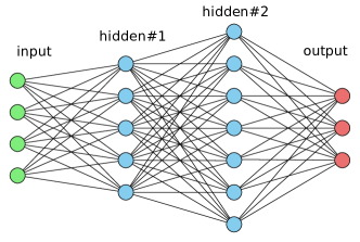
Figure 1: An exemplary MLP with one input layer, two hidden layers and one output layer.

As compared with traditional pattern recognition techniques based on simple linear analysis (e.g, linear discriminant analysis, principal component analysis, etc.), MLPs provide a more flexible mapping from the feature space to the decision space, where the distribution of feature points of one class can be non-convex and irregular. It is built upon a solid theoretical foundation proved by Cybenko [4] and Hornik et al. [5]. That is, a network with only one hidden layer can be a universal approximator if there are “enough” neurons.

Convolutional Neural Networks (CNNs). Fukushima’s Neocognitron [6] can be viewed as an early form of a CNN. The architecture introduced by LeCun et al. in [7] serves as the basis of modern CNNs. The main difference between MLPs and CNNs lies in their input space - the former are features while the latter are source data such as image, video, speech, etc. This is not a trivial difference. Let us use the LeNet-5 shown in Fig. 2 as an example, whose input is an image of size 32 by 32. Each pixel is an input node. It would be very challenging for an MLP to handle this input since the dimension of the input vector is $32\times 32=1,024$. The diversity of possible visual patterns is huge. As explained later, the nodes in the first hidden layer should provide a good representation for the input signal. Thus, it implies a large number of nodes in hidden layers. The number of links (or filter weights) between the input and the first hidden layers is $N_{0}\times N_{1}$ due to full connection. This number can easily go to the order of millions. If the image dimension is in the order of millions such as those captured by the smart phones nowadays, the solution is clearly unrealistic.

Instead of considering interactions of all pixels in one step as done in the MLP, the CNN decomposes an input image into smaller patches, known as receptive fields for nodes at certain layers. It gradually enlarges the receptive field to cover a larger portion of the image. For example, the filter size of the first two convolutional layers of LeNet-5 is $5\times 5$. The first convolutional layer considers interactions of pixels in the short range. Since the patch size is small, the diversity is less. One can use 6 filters to provide a good approximation to the $5\times 5$ source patches, and all source patches share the same 6 filters regardless of their spatial location. After subsampling, the second convolutional layer examines interaction of pixels in the mid-range. After another subsampling, the whole spatial domain is shrinked to a size $5\times 5$ so that it can take global interaction into account using full connection. Typically, the interaction contains not only spatial but also spectral elements (e.g. the RGB three channels and multiple filter responses at the same spatial location) and all interactions are modeled by computational neurons as given in Eq. (1).

It is typical to decompose a CNN into two sub-networks: the feature extraction (FE) subnet and the decision making (DM) subnet. The FE subnet consists of multiple convolutional layers while the DM subnet is composed by a couple of fully connected layers. Roughly speaking, the FE subnet conducts clustering aiming at a new representation through a sequence of RECOS transforms. The DM subnet links data representations to decision labels, which is similar to the classification role of MLPs. The exact boundary between the FE subnet and the DM subnet is actually blurred in the LeNet-5. It can be either S4 or C5 . If we view S4 as the boundary, then C5 and F6 are two hidden layers of the DM subnet. On the other hand, if we choose C5 as the boundary, then there is only one hidden layer (i.e., F6) in the DM subnet. Actually, since these two subnets are connected side-by-side, the transition from the representation to the classification happens gradually and smoothly.

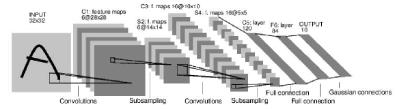
Figure 2: The LeNet-5 architecture [7] as an exemplary CNN.

One main advantage of CNNs over the state vector machine (SVM) and the random forest (RF) classifiers is that the feature extraction task is automatically done through the BP from the last layer to the first layer. Generally speaking, discriminant features are difficult to find for traditional classifiers such as the MLP, SVM and RF. Such tasks, called the feature engineering, demand the domain knowledge. Furthermore, it is difficult to argue that ad hoc features found empirically are optimal in any sense. This explains why the traditional computer vision field is fragmented by different applications. After the emergence of CNNs, the domain knowledge is no more important in feature extraction, yet it plays a critical role in data labeling (known as the label engineering). To give an example, anaconda, vipers, titanoboa, cobras, rattlesnake, etc. are finer classifications of snakes. It demands expert knowledge to collect and label their images. The CNN provides a powerful tool in data-driven supervised learning, where the emphasis is shifted from “extracting features from the source data” to “constructing datasets by pairing carefully selected data and their labels”.

-B Single-Layer RECOS Transform

Our discussion applies to ${\bf x}$ and ${\bf a}$ if $\mu=0$ or augmented vectors ${\bf x^{\prime}}$ and ${\bf a^{\prime}}$ if $\mu\neq 0$. For convenience, we only consider the case with $\mu=0$. The generalization to $\mu\neq 0$ is straightforward.

Clustering on Sphere’s Surface. There is a modern interpretation to the function of a single perceptron layer based on the clustering notion. Since data clustering is a well understood discipline, one can understand the operation of CNNs better if a connection between the operation of a perceptron layer and data clustering can be established. This link was built in [1]. It will be repeated below. Let

$$S=\left\{{\bf x}\biggr{\rvert}||{\bf x}||=1\right\}.$$

be an $N$-dimensional unit hyper-sphere (or simply sphere). We consider clustering of points in $S$ using the geodesic distance. For an arbitrary vector ${\bf x}$ to be a member in $S$, we need to normalize it by its magnitude $g=||{\bf x}||$. If ${\bf x}$ is an image patch, the magnitude normalization after its mean removal has a physical meaning; namely, contrast adjustment. When $g$ is smaller than a threshold, the patch is nearly flat. A flat patch carries little visual information yet its normalization does amplify noise. In this case, it is better to treat it as a zero vector. When $g$ is larger than the threshold, vector ${\bf x}$ does represent a visual pattern and humans perceive little difference between the original and normalized patches since the contrast has little effect on visual patterns. Although this normalization procedure is not implemented in today’s CNNs, the following mathematical analysis can be significantly simplified while the essence of CNNs can still be well captured.

The geodesic distance of two points, ${\bf x}_{i}$ and ${\bf x}_{j}$ in $S$, is proportional to the magnitude of their angle, which can be computed by

$$\theta({\bf x}_{i},{\bf x}_{j})=\cos^{-1}({\bf x}^{T}_{i}{\bf x}_{j}).$$

Since $\cos\theta$ is a monotonically decreasing function for $0^{o}\leq|\theta|\leq 180^{o}$, we can use the correlation, $0\leq{\bf x}_{i}^{T}{\bf x}_{j}=\cos\theta\leq 1$, as another distance measure between them, and cluster vectors in $S$ accordingly. Note that, when $90^{o}\leq|\theta|\leq 180^{o}$, the correlation, ${\bf x}^{T}_{i}{\bf x}_{j}=\cos\theta$, is a negative value.

For MLPs and CNNs, a set of neurons is used to operate on a set of input nodes. For example, nodes in each hidden layer and the output layer in Fig. 1 take the weighted sum of values of nodes in the preceding layer as their outputs. These outputs are treated as one inseparable unit which becomes the input to the next layer. Each neuron has a filter weight vector denoted by ${\bf a}_{k}$, $k=1,\cdots,K$. In the signal processing terminology, the set of neurons forms a filter bank. The “REctified-COrrelations on a Sphere” (RECOS) model [1] describes the relationship between nodes of the $(l-1)$th and $l$th layers, $l=1,2,\cdots$, where the input layer is the $0$th layer. There are three RECOS units in cascade for the MLP in Fig. 1. One corresponds to a filter bank. The filter weight vector is called an anchor vector since it serves as a reference pattern associated with a neuron unit.

Need of Rectification. A neuron computes the correlation between an input vector and its anchor vector to measure their similarity. There are $K$ neurons in one RECOS unit. The projection of ${\bf x}$ onto all anchor vectors, ${\bf a}_{k}$, can be written in form of

$${\bf y}={\bf A}{\bf x},\quad{\bf A}^{T}=[{\bf a}_{1}\cdots{\bf a}_{k}\cdots{\bf a}_{K}],$$

where ${\bf y}=(y_{1},\cdots,y_{k},\cdots y_{K})^{T}\in R^{K}$, $y_{k}={\bf a}_{k}^{T}{\bf x}$ and ${\bf A}\in R^{K\times N}$. For input vectors ${\bf x}_{i}$ and ${\bf x}_{j}$, their corresponding outputs are ${\bf y}_{i}$ and ${\bf y}_{j}$. If the geodesic distance of ${\bf x}_{i}$ and ${\bf x}_{j}$ in $S$ is close, we expect the distance of ${\bf y}_{i}$ and ${\bf y}_{j}$ in the $K$-dimensional output space to be close as well.

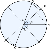
Figure 3: Illustrate the need of rectification [1].

To show the necessity of rectification, a 2D example is illustrated in Fig. 3, where ${\bf x}$ and ${\bf a}_{k}$ ($k=1,2,3$) denote an input and three anchor vectors on the unit circle, respectively, and $\theta_{i}$ is their respective angle. Since $\theta_{1}$ and $\theta_{2}$ are less than 90 degrees, ${\bf a}^{T}_{1}{\bf x}$ and ${\bf a}^{T}_{2}{\bf x}$ are positive. The angle, $\theta_{3}$, is larger than 90 degrees and correlation ${\bf a}^{T}_{3}{\bf x}$ is negative. The two vectors, ${\bf x}$ and ${\bf a}_{3}$, are far apart in terms of the geodesic distance. Since $\cos\theta$ is monotonically decreasing for $0^{o}\leq|\theta|\leq 180^{o}$, it can be used to reflect the order of the geodesic distance in one layer.

However, when two RECOS units are in cascade, the filter weights of the 2nd RECOS unit can take positive or negative values. If the response of the 1st RECOS unit is negative, the product of a negative response and a negative filter weight will produce a positive value. On the other hand, the product of a positive response and a positive filter weight will also produce a positive value. If the nonlinear activation unit did not exist, the cascaded system would not be able to differentiate them. For example, the geodesic distance of ${\bf x}$ and ${\bf-x}$ should be farthest. However, they yield the same result and their original patches become indistinguishable under this scenario. Similarly, a system without rectification cannot differentiate the following two cases: 1) a positive response at the first layer followed by a negative filter weight at the second layer; and 2) a negative response at the first layer followed by a positive filter weight at the second layer.

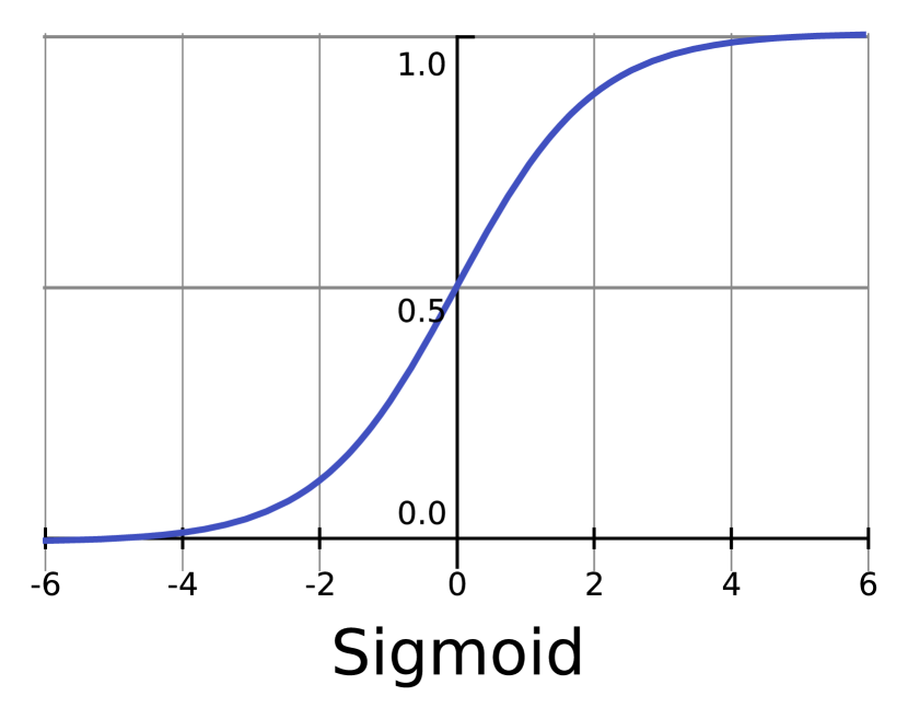
(a)

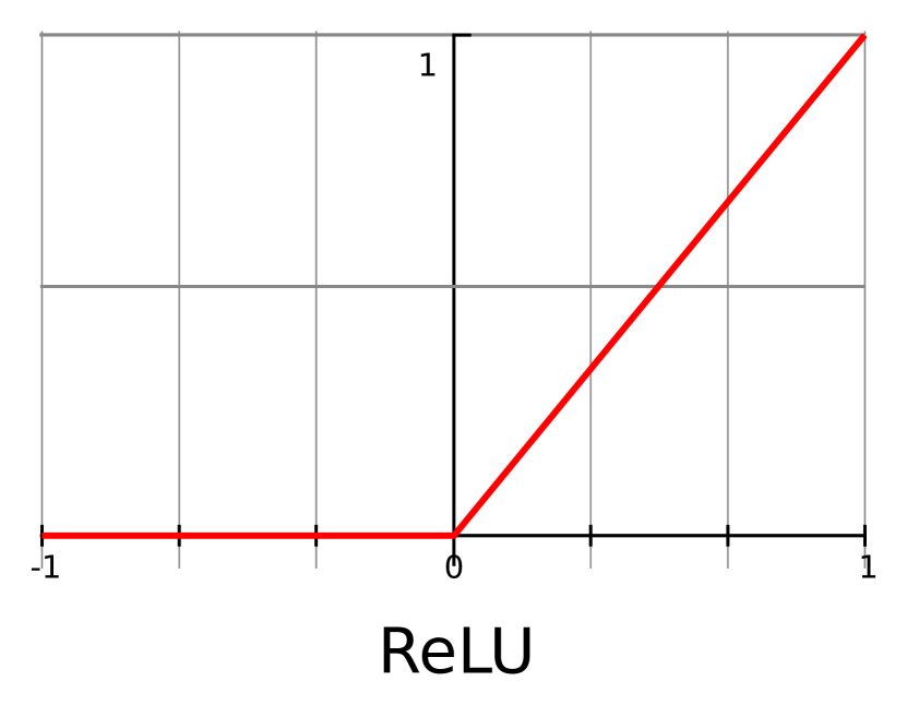
(b)

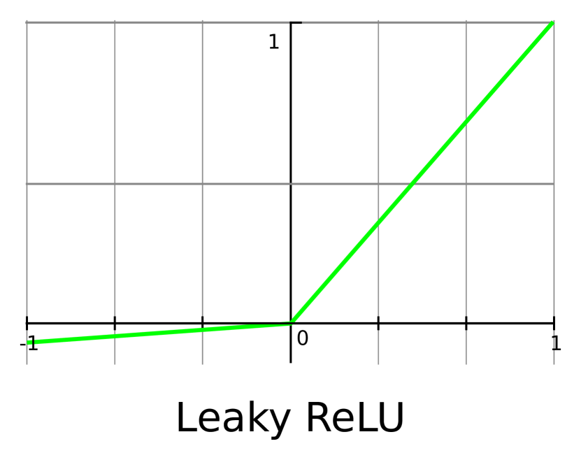
(c)

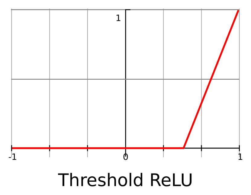
(d)

Figure 4: Illustration of four rectifiers: (a) the sigmoid function, (b) the ReLU (middle), (c) the Leaky ReLU and (d) the Threshold ReLU.

Rectifier Design. Since a nonlinear activation unit is used to rectify correlations, it is called a rectifier here. To avoid the above-mentioned confusion cases, we impose the following two requirements on a rectifier.

1. The output ${\bf a}^{T}_{k}{\bf x}$ should be rectified to be a non-negative value.

2. The rectification function should be monotonically increasing so as to preserve the order of the geodesic distance.

Three rectifiers are often used in MLPs and CNNs. They are the sigmoid function, the rectified linear unit (ReLU) and the parameterized ReLU (PReLU) as shown in Figs. 4(a)-(c). The PReLU is also known as the leaky ReLU. Both the sigmoid and ReLU satisfy the above two requirements. Although the PReLU does not satisfy the first requirement strictly, it does not have a severe negative impact on spherical surface clustering. This is because a negative correlation is rectified to a significantly smaller negative value.

Based on the two requirements, one can design different rectifiers. One example is shown in Fig. 4(d). It is called the threshold ReLU (TReLU). The rectification function can be defined as $\mbox{TReLU}(x)=0$, if $x<\phi$ and $\mbox{TReLU}(x)=\frac{x-\phi}{1-\phi}$ if $x\geq\phi$. When $\phi=0$, TReLU is reduced to ReLU. For the LeNet-5 applied to the MNIST dataset, we observe better performance as $\phi$ increases from 0 to 0.5 and then decreases. One advantage of $\mbox{TReLU}(\phi)$ with $\phi>0$ is that we can block the influence of more anchor vectors. When $\phi=0$, we block the influence of anchor vectors that have an angle larger than 90 degrees with respect to the input vector. When $\phi=0.5$, we block the influence of anchor vectors that have an angle larger than 60 degrees. The design of an optimal rectifier for target applications remains to be an open problem.

-C Multi-layer RECOS Transform

Single-Layer Signal Analysis via Representation. Signal modeling and representation is commonly used in the signal processing field for signal analysis. Typically, we have a linear model in form of

$${\bf x}={\bf A}{\bf c},$$ (2)

where ${\bf x}\in R^{N}$ denotes the signal of interest, ${\bf A}\in R^{N\times M}$ is a representation matrix and ${\bf c}\in R^{M}$ is the coefficient vector. If $M=N$ and the column vectors of ${\bf A}$ form a set of basis functions, Eq. (2) defines a transform from one basis to another. The task is in selecting powerful basis functions to represent signals of interest. Fourier and wavelet transforms are well known examples. Then, a subset of coefficient vector ${\bf c}$ can be used as the feature vector. If $M>N$, there exist infinitely many solutions in ${\bf c}$. We can impose constraints on ${\bf c}$, leading to the linear least-squares solution, sparse coding, among others. For the sparse representation, the task is in finding a good dictionary, ${\bf A}$, to represent the underlying signal effectively. Again, a subset of coefficient vector ${\bf c}$ can be chosen as features.

Multi-Layer Signal Analysis via Cascaded Transforms. The CNN approach provides a brand new framework for signal analysis. Instead of finding a representation for signal analysis, it relies on a sequence of cascaded transforms that builds a link between the input signal space and the output decision space. The operation at each layer is to conduct spherical surface’s clustering of input samples with a rectified output (i.e. the RECOS transform).

For MLPs, each network corresponds to a simple cascade of multiple RECOS transforms. Mathematically, we have

$${\bf d}={\bf B}_{L}\cdots{\bf B}_{l}\cdots{\bf B}_{1}{\bf x},$$ (3)

where ${\bf x}$ is an input signal, ${\bf d}=(d_{1},\cdots,d_{c},\cdots,d_{C})$ is an output vector in the decision space indicating the likelihood in class $c$ with $c=1,\cdots,C$, and ${\bf B}_{l}$ is the $l$th layer RECOS transform matrix with $l=1,\cdots,L$. The input and output to the $l$th layer RECOS transform ${\bf B}_{l}$ are denoted by ${\bf x}_{l-1}$ and ${\bf x}_{l}$, respectively. Thus, we get

$${\bf x}_{l}={\bf B}_{l}{\bf x}_{l-1},\quad\mbox{where}\quad{\bf B}_{l}={\bf R}\circ{\bf A}_{l},$$ (4)

and where ${\bf R}$ is the element-wise rectification function operating on the output of ${\bf A}_{l}{\bf x}_{l-1}$. Clearly, we have ${\bf x}_{0}={\bf x}$ and ${\bf x}_{L}={\bf d}$.

The ground truth ${\bf d}$ is that $d_{i}=1$ if $i$ is the target class while $d_{j}=0$ if $j$ is not the target class. It is called the one-hot vector. The training samples have both input ${\bf x}$ and its label ${\bf d}$. The testing samples have only input ${\bf x}$, and we need to predict its output ${\bf d}$ and convert it to its nearest one-hot vector. The task is in finding good ${\bf B}_{l}$, $l=1,\cdots,L$, so as to minimize the classification error.

For CNNs, we have two types of ${\bf B}_{l}$ in form of:

$${\bf B}_{l}^{C}={\bf P}\bigcup_{s\in\Omega}{\bf R}\circ{\bf A}_{l,s},\quad\mbox{and}\quad{\bf B}_{l}^{F}={\bf R}\circ{\bf A}_{l},$$ (5)

where ${\bf A}_{l,s}$ denotes a convolutional filter at layer $l$ with spatial index $s$, $\bigcup_{s}$ is the union of outputs from a neighborhood, $\Omega$, and ${\bf P}$ denotes a pooling operation. The union of outputs from a set of parallel convolutional filters serve as the input to the filter at the next layer. The two RECOS transforms, ${\bf B}_{l}^{C}$ and ${\bf B}_{l}^{F}$, are called the convolutional layer and the fully connected layer, respectively, in the modern CNN literature. Clearly, ${\bf B}_{l}={\bf B}_{l}^{F}$ in Eq. (4).

It is inspiring to compare the two signal analysis approaches as given in Eqs. (2) and (3). The one in Eq. (2) is a single layer approach where no rectification is needed. The one in Eq. (3) is a multi-layer approach and rectification is essential. The single layer approach seeks for a better signal representation. For example, a multiple-scale signal representation was developed using the wavelet transform. A sparse signal representation was proposed using a trained dictionary. The objective is to find an “optimal” representation to separate critical components in desired signals from others.

In contrast, the CNN approach does not intend to decompose underlying signals. Instead, it adopts a sequence of RECOS transforms to cluster input data based on their similarity layer by layer until the output layer is reached. The output layer predicts the likelihood of all possible decisions (e.g., object classes). The training samples provide a relationship between an image and its decision label. The CNN can predict results even without any supervision, although the prediction accuracy would be low. The training samples guide the CNN to form more suitable anchor vectors (thus better clusters) and connect clustered data with decision labels. To summarize, we can express the multi-layer RECOS transform as

MLP: $${\bf x}={\bf x}_{0}\overset{{\bf B}_{1}^{F}}{\longrightarrow}{\bf x}_{1}\overset{{\bf B}_{2}^{F}}{\longrightarrow}\cdots\overset{{\bf B}_{L-1}^{F}}{\longrightarrow}{\bf x}_{L-1}\overset{{\bf B}_{L}^{F}}{\longrightarrow}{\bf x}_{L}={\bf d},$$

CNN: $${\bf x}={\bf x}_{0}\overset{{\bf B}_{1}^{C}}{\longrightarrow}{\bf x}_{1}\overset{{\bf B}_{2}^{C}}{\longrightarrow}\cdots\overset{{\bf B}_{m}^{C}}{\longrightarrow}{\bf x}_{m}\overset{{\bf B}_{m+1}^{F}}{\longrightarrow}{\bf x}_{m+1}\overset{{\bf B}_{m+2}^{F}}{\longrightarrow}\cdots\overset{{\bf B}_{L-1}^{F}}{\longrightarrow}{\bf x}_{L-1}\overset{{\bf B}_{L}^{F}}{\longrightarrow}{\bf x}_{L}={\bf d},$$

The output from the $l$th layer, ${\bf x}_{l}$, serves as the input to the $(l+1)$th layer. It is called the intermediate representation at the $l$th layer or the $l$th intermediate representation in short.

It is important to have a deeper understanding on the compound effect of two RECOS transforms in cascade. This was thoroughly studied in [1], and the main result is summarized below. A representative 2D input and its corresponding anchor vectors are shown in Fig. 5. Let ${\boldsymbol{\alpha}}_{n}$ be a $K$-dimensional vector formed by the same position (or element) of ${\bf a}_{k}$. It is called the anchor-position vector since it captures the position information of anchor vectors. Although anchor vectors ${\bf a}_{k}$ capture global representative patterns of ${\bf x}$, they are weak in capturing position sensitive information. This shortcoming can be compensated by modulating outputs with elements of anchor-position vector ${\boldsymbol{\alpha}}_{n}$ in the next layer.

Let us use layers S4, C5 and F6 in LeNet-5 as an example. There are $120$ anchor vectors of dimension $400$ from S4 to C5. We collect $400$ anchor-position vectors of dimension $120$, multiply the output at C5 by them to form a set of modulated outputs, and then compute $84$ anchor vectors of dimension $120$ from C5 to F6. Note that the output at C5 contains primarily the spectral information but not the position information. If a position in the input vectors has less consistent information, the variance of its associated anchor position vector will be larger and the modulated output will be more random. As a result, its impact on the formation of the $84$ anchor vectors is reduced. For more details, we refer to the discussion in [1].

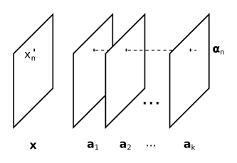
Figure 5: Visualization of anchor-position vector ${\boldsymbol{\alpha}}_{n}$ [1].

New Clustering Representation. We have a one-to-one association between a data sample and its cluster in traditional clustering schemes. However, this is not the case in the RECOS transform. A new clustering representation is adopted by MLPs and CNNs. That is, for an input vector ${\bf x}$, the RECOS transform generates a set of $K$ non-negative correlation values as the output vector of dimension $K$. This representation enables repetitive clustering layer by layer as given in Eq. (4). For an input, one can determine the significance of clusters according to the magnitude of the rectified output value. If its magnitude for a cluster is zero, ${\bf x}$ is not associated with that cluster. A cluster is called a relevant or irrelevant one depending on whether it has an association with ${\bf x}$. Among all relevant ones, we call cluster $i$ the “primary” cluster for input ${\bf x}$ if

$$i=\mbox{arg}\max_{k}{\bf a}_{k}^{T}{\bf x}.$$

The remaining relevant ones are “auxiliary” clusters.

The FE subnet uses anchor vectors to capture local, mid-range and long-range spatial patterns. It is difficult to predict the clustering structure since new information is introduced at a new layer. The DM subnet attempts to reduce the dimension of intermediate representations until it reaches the dimension of the decision space. We observe that the clustering structure becomes more obvious as the layer of the DM subnet goes deeper. That is, the output value from the primary cluster is closer to unity while the number of auxiliary clusters is fewer and their output values become smaller. When this happens, an anchor vector provides a good approximation to the centroid for the corresponding cluster.

The choice of anchor vector numbers, $K_{l}$, at the $l$th layer is an important problem in the network design. If input data ${\bf x}_{l-1}$ has a clear clustering structure (say, with $h$ clusters), we can set $K_{l}=h$. However, this is often not the case. If $K_{l}$ is set to a value too small, we are not able to capture the clustering structure of ${\bf x}_{l-1}$ well, and it will demand more layers to split them. If $K_{l}$ is set to a value too large, there are more anchor vectors than needed and a stronger overlap between rectified output vectors will be observed. As a result, we still need more layers to separate them. Another way to control the clustering process is the choice of the threshold value, $\phi$, of the TReLU. A higher threshold value can reduce the negative impact of a larger $K_{l}$ value. The tradeoff between $\phi$ and $K_{l}$ is an interesting future research topic.

The interpretation of a CNN as a guided multi-layer RECOS transform is helpful in understanding the CNN self-organization capability as discussed below.

-D Network Initialization and Guided Anchor Vector Update

Data clustering plays a critical role in the understanding of the underlying structure of data. The k-means algorithm, which is probably the most well-known clustering method, has been widely used in pattern recognition and supervised/unsupervised learning. As discussed earlier, each CNN layer conducts data clustering on the surface of a high-dimensional sphere based on a rectified geodesic distance. Here, we would like to understand the effect of multiple layers in cascade from the input data source to the output decision label. For unsupervised learning such as image segmentation, several challenges exist in data clustering [8]. Questions such as “what is a cluster?” “how many clusters are present in the data?” “are the discovered clusters and partition valid?” remain open. These questions expose the limit of unsupervised data clustering methods.

In the context of supervised learning, traditional feature-based methods extract features from data, conduct clustering in the feature space and, finally, build a connection between clusters and decision labels. Although it is relatively easy to build a connection between the data and labels through features, it is challenging to find effective features. In this setting, the dimension of the feature space is usually significantly smaller than that of the data space. As a consequence, it is unavoidable to sacrifice rich diversity of input data. Furthermore, the feature selection process is guided by humans based on their domain knowledge (i.e. the most discriminant properties of different objects). This process is heuristic. It can get overfit easily. Human efforts are needed in both data labeling and feature design.

CNNs offer an effective supervised learning solution, where supervision is conducted by a training process using data labels. This supervision closes the semantic gap between low-level representations (e.g., the pixel representation) and high-level semantics. Furthermore, the CNN self-organization capability was well discussed in 80s and 90s, e.g., [6]. By self-organization, the network can learn with little supervision. To put the above two together, we expect that CNNs can provide a wide range of learning paradigms – from the unsupervised, weakly supervised to heavily supervised learning. This intuition can be justified by considering a proper anchor vector initialization scheme (for self-organization) and providing proper “guidance” to the proposed multi-layer RECOS transform in anchor vector update (for supervised learning).

Network Initialization. The CNN conducts a sequence of representation transforms using cascaded RECOS units. The dimension of transformed representations gradually decreases until it reaches the number of output classes. Since labels of output classes are provided by humans with a semantic meaning, the whole end-to-end process is called the guided (or supervised) transform.

Before examining the effect of label guidance, we first compare two network initialization schemes: 1) the random initialization and 2) the k-means initialization. For the latter, we perform k-means at each layer based on its corresponding input data samples (with zero-mean and unit-length normalization), and repeat this process from the input to the output layer after layer. Random initialization is commonly adopted nowadays. Based on the above discussion, we expect the k-means initialization to be a better choice. This is verified by our experiments in the LeNet-5 applied to the MNIST dataset.

Once the network is initialized, we can feed the test data to the network and observe the output, which corresponds to unsupervised learning. The comparison of unsupervised classification results with the random and k-means initializations is given in Fig. 6, where we show images that are closest to the anchor vectors (or centroids) of the ten output nodes. We see that the k-means initialization provides ten anchor vectors pointing to ten different digits while the random initialization cannot do the same. Different random initialization schemes will lead to different results, yet the one given in Fig. 6 is representative. That is, multiple anchor vectors will point to the same digit.

Guided Anchor Vector Update. We apply the BP for network training with a varying number of training samples. For a fixed number of training samples, we train the network until its performance converges and plot the correct classification rate in Fig. 7. The two points along the y-axis indicate the correct classification rates without any training sample. The rates are around 32% and 14% for the k-means and random initializations, respectively. Note that the 14% is slightly better than the random guess on the outcome, which is 10%. Then, both performance curves increase as the number of training samples grows. The k-means can reach a correct classification rate of 90% when the number of training samples is around 250, which is only 0.41% of the entire MNIST training dataset (i.e. 60K samples). This shows the power of the LeNet-5 even under extremely low supervision.

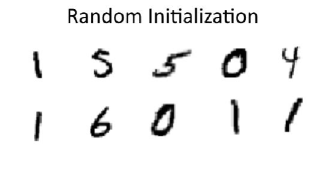
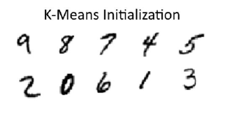
Figure 6: Comparison of MNIST unsupervised classification results of the LeNet-5 architecture with the random (left) and k-means (right) initializations, where the images that are closest to centroids of ten output nodes are shown.

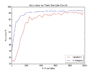
Figure 7: Comparison of MNIST weakly-supervised classification results of the LeNet-5 architecture with the random and k-means initializations, where the correct classification rate is plotted as a function of training sample numbers.

To further understand the role played by label guidance, we examine the impact of the BP on the orientation of anchor vectors in various layers. We show in Table I the averaged orientation changes of anchor vectors in terms of radian (or degree) for the two cases in Fig. 6. They are obtained after the convergence of the network with all 60,000 MNIST training samples. This orientation change is the result due to label guidance through the BP. It is clear from the table that, a good network initialization (corresponding to unsupervised learning) leads to a faster convergence rate in supervised learning.

In/Out layers	k-means	random
Input/S2	0.155 (or $8.881^{o}$)	1.715 (or $98.262^{o}$)
S2/S4	0.169 (or $9.683^{o}$)	1.589 (or $91.043^{o}$)
S4/C5	0.204 (or $11.688^{o}$)	1.567 (or $89.783^{o}$)
C5/F6	0.099 (or $5.672^{o}$)	1.579 (or $90.470^{o}$)
F6/Output	0.300 (or $17.189^{o}$)	1.591 (or $91.158^{o}$)

TABLE I: The averaged orientation changes of anchor vectors in terms of the radian (or degree) for the k-means and the random initialization schemes.

Classes and Sub-Classes. We use another example to gain further insights to the guided clustering process. We can zoom into the horned rattlesnake class obtained by the AlexNet and conduct the unsupervised k-means on feature vectors in the last layer associated with this class to further split it into multiple sub-classes. Images of two sub-classes are shown in Fig. 8. Images in the same sub-classes are visually similar. However, they are not alike across sub-classes. The two sub-classes are grouped together under the horned rattlesnake class because they share the same class label (despite strong visual dissimilarity). That shows the power of label guidance. However, the feature distance is shorter for images in the same sub-class and longer for images in different sub-classes. This is due to the inherent clustering capability of CNNs.

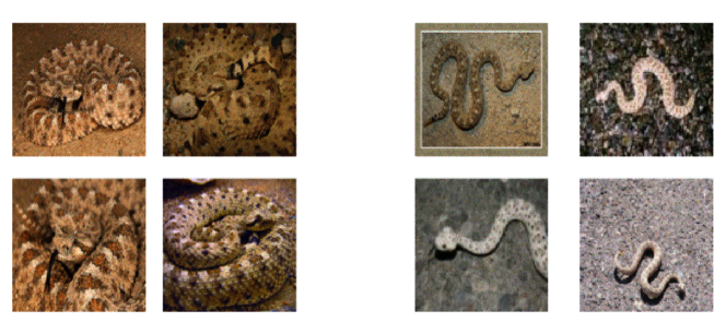
Figure 8: Two sub-classes obtained from the horned rattlesnake class using unsupervised clustering.

-E Discussion and Open Issues

Discussion. A CNN was viewed as a guided multi-layer RECOS transform in this note. The following known facts can also be explained using this interpretation.

• Robustness to wrong labels. Humans do clustering first and then the CNN mimics humans based on the statistics of all labeled samples. It can tolerate small percentages of erroneous labels since these wrongly labeled data do not have a major impact on clustering results.

• Overfitting. Overfitting occurs when a statistic model describes noise instead of the underlying input/output relationship. For a given number of observations, this could happen for an excessively complex model that has too many model parameters. Such a model has poor prediction performance since it over reacts to minor fluctuations in the training data. Although a CNN has a large number of parameters (namely, filter weights), it does not suffer much from overfitting for the following reason. When there are only input and output layers without any hidden layers in between, the CNN solves a linear least-squared regression problem (where no rectification is needed.) It is well known the linear regression is robust to noisy data. When there are hidden layers, the filter weight determination is a cascaded optimization problem, which has to be solved iteratively. In the BP process, we update the filter weights layer by layer in a backward direction. Fundamentally, it still attempts to solve a regression problem at each layer. Although a rectifier conducts rectification on the output, it does not change the regression nature of MLPs and CNNs.

• Data augmentation. A low-cost way to generate more samples is data augmentation. This is feasible since minor perturbations in the image pixel domain do not change their class types.

• Dataset bias. A CNN can be biased due to the inherent bias in the low level representation existing in training samples. Thus, the performance of a CNN can degrade significantly from one dataset to the other in the same application domain due to this reason.

Open Issues. There are many interesting open problems remaining for further exploration.

• Network Architecture Design. It is interesting to be able to specify the layer number and the filter number per layer for given applications automatically.

• Decoder Network Analysis. The classification network maps an image to a label. There are image processing networks that accept an image as the input and another image as the output. Examples include super-resolution networks, semantic segmentation networks, etc. These networks can be decomposed into an encoder-decoder architecture. The analysis in this note focuses on the encoder part. It is interesting to generalize the analysis to the decoder part as well.

• Localization and Attention. Region proposals have been used in object detection to handle the object localization problem. It is desired to learn the object location and human visual attention from the network automatically without the use of proposals. The design and analysis of networks to achieve this goal is interesting.

• Transfer Learning. It is often possible to finetune a CNN for a new application based on an existing CNN model trained by another dataset in another application. This is because the low-level image representation corresponding to the beginning CNN layers can be very flexible and equally powerful.

• Weakly Supervised Learning. Unsupervised and Heavily supervised learning are two extremes. Weakly supervised learning occurs most frequently in our daily applications. The design and analysis of a weakly supervised learning mechanism based on CNNs is interesting and practical.

The interpretation of a CNN as a guided multi-layer RECOS transform should be valuable to the investigation of these topics.

CONCLUSION

The operating principle of CNNs was explained as a guided multi-layer RECOS transform in this note. A couple of illustrative examples were provided to support this claim. Several known facts were interpreted accordingly, and some open issues were pointed out at the end.

AUTHOR

C.-C. Jay Kuo (cckuo@ee.usc.edu) is a Professor of Electrical Engineering at the University of Southern California, Los Angeles, California, USA.

References

- [1] C.-C. J. Kuo, “Understanding convolutional neural networks with a mathematical model,” Journal of Visual Communication and Image Representation, vol. 41, pp. 406–413, 2016.
- [2] W. S. McCulloch and W. Pitts, “A logical calculus of the ideas immanent in nervous activity,” The Bulletin of Mathematical Biophysics, vol. 5, no. 4, pp. 115–133, 1943.
- [3] F. Rosenblatt, “The perceptron: a probabilistic model for information storage and organization in the brain,” Psychological Review, vol. 65, no. 6, pp. 386–408, 1957.
- [4] G. Cybenko, “Approximation by superpositions of a sigmoidal function,” Mathematics of Control, Signals and Systems, vol. 2, no. 4, pp. 303–314, 1989.
- [5] K. Hornik, M. Stinchcombe, and H. White, “Multilayer feedforward networks are universal approximators,” Neural Networks, vol. 2, no. 5, pp. 359–366, 1989.
- [6] K. Fukushima, “Neocognitron: a self-organizing neural network model for a mechanism of pattern recognition unaffected by shift in position,” Biological Cybernetics, vol. 36, pp. 193–202, 1980.
- [7] Y. LeCun, L. Bottou, Y. Bengio, and P. Haffner, “Gradient-based learning applied to document recognition,” Proc. IEEE, vol. 86, no. 11, pp. 2278–2324, 1998.
- [8] A. K. Jain, “Data clustering: 50 years beyond k-means,” Pattern Recognition Letters, vol. 31, no. 8, pp. 651–666, 2010.