Dimensional crossover in a strongly interacting ultracold atomic Fermi gas

Abstract

We theoretically explore the crossover from three dimensions (3D) to two (2D) in a strongly interacting atomic Fermi superfluid through confining the transverse spatial dimension. Using the gaussian pair fluctuation theory, we determine the zero-temperature equation of state and Landau critical velocity as functions of the spatial extent of the transverse dimension and interaction strength. In the presence of strong interactions, we map out a dimensional crossover diagram from the location of maximum critical velocity, which exhibits distinct dependence on the transverse dimension from 2D to quasi-2D, and to 3D. We calculate the dynamic structure factor to characterize the low-energy excitations of the system and propose that the intermediate quasi-2D regime can be experimentally probed using Bragg spectroscopy.

Recent breakthroughs in understanding strongly interacting ultracold atomic Fermi gases at the crossover from Bose-Einstein condensates (BEC) to Bardeen-Cooper-Schrieffer (BCS) superfluids Eagles1969 ; Leggett1980 ; NSR1985 ; SadeMelo1993 have attracted enormous attention from diverse fields of physics MBX1999 ; Giorgini2008 ; Randeria2014 . Due to the unprecedented accuracy in controlling the dimensionality and interatomic interaction Bloch2008 ; Chin2010 , significant progress has been made to realize systems in the 2D limit Martiyanov2010 ; Feld2011 ; Frohlich2011 ; Dyke2011 ; Orel2011 ; Koschorreck2012 ; Sommer2012 ; Zhang2012 ; Makhalov2014 ; Ong2015 ; Ries2015 ; Murthy2015 ; Dyke2016 ; Martiyanov2016 ; Fenech2016 ; Boettcher2016 ; Cheng2016 . It thus provides a new paradigm to explore a number of intriguing low-dimensional phenomena, including the absence of a true long-range order at nonzero temperature Mermin1966 ; Hohenberg1967 , the existence of quasi-condensates due to the Berezinskii-Kosterlitz-Thouless mechanism Berezinskii1972 ; KT1973 ; Salasnich2013 , the disruptive role of pair fluctuations around the mean-field (MF) Randeria1989 ; SchmittRink1989 ; Engelbrecht1990 ; Watanabe2013 ; Bauer2014 ; Marsiglio2015 ; He2015 ; Mulkerin2015 ; Bighin2016 , and the possible observation of exotic imbalanced superfluidity Conduit2008 ; Yin2014 ; Toniolo2017 . These unusual features lie at the heart of many technologically interesting materials such as high-temperature superconductors Lee2006 , where the dimensional crossover from 3D to 2D is dictated by the ratio of the Cooper pair size to the thickness of the superconducting layer.

Despite rapid experimental advances, the fundamental criteria for reaching the strict 2D regime at the BEC-BCS crossover are still not well understood. Experimentally, a 2D Fermi gas is realized by freezing the atomic motion in the transverse direction using a single highly-oblate harmonic trap Dyke2011 ; Fenech2016 or a tight one-dimensional optical lattice Martiyanov2010 ; Feld2011 ; Sommer2012 ; Zhang2012 ; Ries2015 . In the absence of interactions, the 2D condition is easy to clarify within the single-particle picture: the chemical potential $\mu$ and temperature $k_{B}T$ of the system should be smaller than the characteristic energy scale $\hbar\omega_{z}$ along the transverse direction, so that all atoms stay in the lowest transverse mode Dyke2011 . With strong interactions, the situation is less clear. Indeed, a recent measurement of time-of-flight expansion indicates that it is difficult to display the strict 2D kinematics when the interaction becomes stronger Dyke2016 . Theoretically, the dimensional crossover of a strongly interacting Fermi gas from 3D to 2D is challenging due to the strong correlations Levinsen2015 . To date, an interacting quasi-2D Fermi gas has only been studied in the highly imbalanced polaron limit Levinsen2012 or by using mean-field approach that is known to break down in the 2D limit Hu2011 ; Fischer2014 .

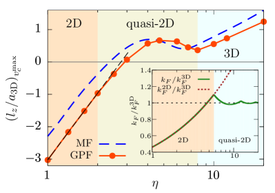
Figure 1: (color online). The dimensional crossover diagram, tuned by the dimension parameter $\eta$ (in logarithmic scale) and the value of the interaction strength, $(l_{z}/a_{\text{3D}})_{v_{c}^{\max}}$, at which the Landau critical velocity peaks. The red solid line (with circles) and blue dashed line show $(l_{z}/a_{\text{3D}})_{v_{c}^{\max}}$ predicted by the GPF and MF theories, respectively. Their distinct dependences on $\eta$ enables us to identify the 2D and 3D regimes, and the quasi-2D regime in between. The inset shows the dimensional crossover diagram in the non-interacting case, determined from the free Fermi gas number equation (see text).

In this Letter, we determine the dimensional crossover diagram (see Fig. 1), by considering a uniform strongly interacting quasi-2D Fermi gas with periodic boundary condition (PBC) in the tightly confined transverse direction. This configuration is motivated by the recent successful production of a box trapping potential that leads to a uniform Bose or Fermi gas in bulk Gaunt2013 ; Mukherjee2016 . We apply a gaussian pair fluctuation (GPF) theory to obtain the zero-temperature equation of state (Fig. 2) Mulkerin2015 and Landau critical velocity (Fig. 3) at the dimensional crossover. For a given dimensional parameter $\eta\equiv k_{F}^{\text{3D}}l_{z}$, where $l_{z}$ is the periodic length of the confining potential in the transverse direction and $k_{F}^{\text{3D}}\equiv(3\pi^{2}n)^{1/3}$ is the three-dimensional (3D) Fermi momentum of the gas with density $n$, we determine the interaction strength at which there is a maximum of the Landau critical velocity footnote , $(l_{z}/a_{\text{3D}})_{v_{c}^{\max}}$, where $a_{{\rm 3D}}$ is the 3D $s$-wave scattering length. A Fermi superfluid is most robust to external excitations at this maximum, which is found, in 3D, close to unitarity Combescot2006 ; Sensarma2006 ; Miller2007 . We obtain a regime where the maximum of the critical velocity in the BEC-BCS crossover depends on the logarithm of $\eta$ for $\eta<2$, denoting a 2D regime (i.e., the long-dashed line in Fig. 1). Also, $(l_{z}/a_{\text{3D}})_{v_{c}^{\max}}$ depends linearly on $\eta$ for $\eta>8$, denoting a 3D regime. The region that links these regimes is defined as quasi-2D and has properties distinct to the 2D and 3D limits.

Theoretical framework. — We start by defining various Fermi momenta. We consider a $s$-wave two-component Fermi gas at zero temperature where the transverse direction is confined with periodic length $l_{z}$, implying the discretization of momentum in the $z$-direction, $k_{z}=2\pi n_{z}/l_{z}$, for any integer $n_{z}$. The Fermi momentum $k_{F}$ of the dimensional crossover system can then be defined as the maximally allowed momentum in the axial direction:

$$n=\frac{1}{2\pi l_{z}}\sum_{n_{z}=-n_{\max}}^{n_{\max}}\left[k_{F}^{2}-\left(\frac{2\pi n_{z}}{l_{z}}\right)^{2}\right],$$ (1)

where $n_{\max}$ is the largest integer smaller than $k_{F}l_{z}/(2\pi)$. It is useful to first examine the dimensional crossover diagram for an ideal Fermi gas, as shown in the inset of Fig. 1. At large $l_{z}$ (or $\eta$), $k_{F}$ approaches the 3D Fermi momentum $k_{F}^{\textrm{3D}}$, as anticipated. In the limit of small $l_{z}$, instead, $k_{F}$ coincides with a 2D Fermi momentum $k_{F}^{\textrm{2D}}\equiv\sqrt{2\pi n_{\textrm{2D}}}=\sqrt{2\eta/(3\pi)}k_{F}^{\textrm{3D}}$, where the column density $n_{\textrm{2D}}\equiv nl_{z}$. An ideal 2D Fermi gas is thus realized when $k_{F}=k_{F}^{\textrm{2D}}$ or $\eta<\sqrt[3]{6}\pi\simeq 5.7$, for which only the lowest transverse mode is occupied. This simple 2D condition is not applicable in the presence of strong interactions, a situation that we shall consider below. A strongly interacting Fermi gas with contact interactions between unlike fermions can be described by a single-channel Hamiltonian density Randeria1989 ; He2015 ; Hu2006 ; Diener2008 ,

$$\mathcal{H}=\sum_{\sigma=\uparrow,\downarrow}\bar{\psi}_{\sigma}(\mathbf{r})\mathcal{H}_{0}\psi_{\sigma}(\mathbf{r})-g\bar{\psi}_{\uparrow}(\mathbf{r})\bar{\psi}_{\downarrow}(\mathbf{r})\psi_{\downarrow}(\mathbf{r})\psi_{\uparrow}(\mathbf{r}),$$ (2)

where $\psi_{\sigma}(\mathbf{r})$ are the annihilation operators for each spin state, $\mathcal{H}_{0}=-\hbar^{2}\nabla^{2}/(2M)-\mu$ is the free Hamiltonian with atomic mass $M$, $\mu$ is the chemical potential, and $g>0$ denotes the bare interaction strength. The contact potential is a convenient choice of interaction, however it needs to be regularized and related to a physical observable of the system. We achieve this by relating the bare interaction strength $g$ to the bound state energy $B_{0}$ Yamashita2014 ,

$$\frac{1}{g}=\sum_{\mathbf{k},k_{z}}\frac{1}{2\left(\epsilon_{\mathbf{k}}+\epsilon_{k_{z}}\right)+B_{0}},$$ (3)

where $\epsilon_{\mathbf{k}}=\hbar^{2}\mathbf{k}^{2}/(2M)$ and the sums on $(\mathbf{k},k_{z})$ carry a volume factor that goes to $(2\pi)^{2}l_{z}$ at the thermodynamic limit. In order to recover the 3D limit, we require the two-body $T$-matrix in the dimensional crossover be equivalent to its 3D counterpart in the limit $l_{z}\rightarrow\infty$. This implies that the binding energy, $B_{0}$, can be analytically related to the 3D scattering length $a_{\text{3D}}$, according to Petrov2001 ; Yamashita2014 ,

$$B_{0}=4\left(\frac{\hbar^{2}}{Ml_{z}^{2}}\right)\textrm{arcsinh}^{2}\left[\frac{e^{l_{z}/\left(2a_{\textrm{3D}}\right)}}{2}\right].$$ (4)

It is also possible to define a 2D binding energy, $\epsilon_{B}^{\text{2D}}\equiv\hbar^{2}/(Ma_{\text{2D}}^{2})$, find the equivalence between the scattering $T$-matrix and the 2D $T$-matrix as $l_{z}\rightarrow 0$, and show analytically that $B_{0}=\epsilon_{B}^{\text{2D}}$ in the 2D limit.

We solve the many-body Hamiltonian Eq. (2) by using the zero-temperature GPF theory, which provides reasonable quantitative predictions for equation of state in both 2D He2015 and 3D Hu2007 ; Hu2010 . The theory takes into account strong pair fluctuations at the gaussian level on top of mean-field solutions Hu2006 ; Diener2008 and hence we separate the thermodynamic potential into two parts: $\Omega=\Omega_{{\rm MF}}+\Omega_{{\rm GF}}$. The mean-field part is He2015 ,

$$\Omega_{\textrm{MF}}=\frac{\Delta^{2}}{g}+\sum_{\mathbf{k},k_{z}}\left(\xi_{\mathbf{k},k_{z}}-E_{\mathbf{k},k_{z}}\right),$$ (5)

where $\smash{\xi_{\mathbf{k},k_{z}}=\epsilon_{\mathbf{k}}+\epsilon_{k_{z}}-\mu}$, $\smash{E_{\mathbf{k},k_{z}}=\sqrt{\xi_{\mathbf{k},k_{z}}^{2}+\Delta^{2}}}$, and the order parameter $\Delta$ is determined self-consistently using the mean-field gap equation, $\Delta\sum_{\mathbf{k},k_{z}}[(\epsilon_{\mathbf{k}}+\epsilon_{k_{z}}+B_{0}/2)^{-1}-E_{\mathbf{k},k_{z}}^{-1}]=0$, ensuring the gapless Goldstone mode Combescot2006 . The pair fluctuation part is given by ($Q\equiv(\mathbf{q},q_{z},\omega)$) He2015 ,

$$\Omega_{\text{GF}}=\sum_{\mathbf{q},q_{z}}\int_{0}^{\infty}\frac{d\omega}{2\pi}\ln\left[\frac{\mathbf{M}_{11}\left(Q\right)\mathbf{M}_{11}\left(-Q\right)-\mathbf{M}_{12}^{2}\left(Q\right)}{\mathbf{M}_{11}^{C}\left(Q\right)\mathbf{M}_{11}^{C}\left(-Q\right)}\right],$$ (6)

with the matrix elements,

$$\mathbf{M}_{11}\left(Q\right) = \frac{1}{g}+\sum_{\mathbf{k},k_{z}}\left(\frac{u_{+}^{2}u_{-}^{2}}{\omega-E_{+}-E_{-}}-\frac{v_{+}^{2}v_{-}^{2}}{\omega+E_{+}+E_{-}}\right),$$

$$\mathbf{M}_{12}\left(Q\right) = \sum_{\mathbf{k},k_{z}}\left(-\frac{u_{+}u_{-}v_{+}v_{-}}{\omega-E_{+}-E_{-}}+\frac{u_{+}u_{-}v_{+}v_{-}}{\omega+E_{+}+E_{-}}\right),$$

$$\mathbf{M}_{11}^{C}\left(Q\right) = \frac{1}{g}+\sum_{\mathbf{k},k_{z}}\frac{u_{+}^{2}u_{-}^{2}}{\omega-E_{+}-E_{-}}.$$ (7)

Here, we use the notations $E_{\pm}\equiv E_{\mathbf{k}\pm\mathbf{q}/2,k_{z}\pm q_{z}/2}$, $u_{\pm}^{2}=(1+\xi_{\mathbf{k}\pm\mathbf{q}/2,k_{z}\pm q_{z}/2}/E_{\mathbf{k}\pm\mathbf{q}/2,k_{z}\pm q_{z}/2})/2$ and $v_{\pm}^{2}=1-u_{\pm}^{2}$ He2015 ; Hu2006 ; Diener2008 . The chemical potential is found by solving the number equation, $n=-\partial\Omega/\partial\mu$.

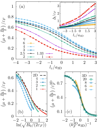
Figure 2: (color online). (a) The dimensionless shifted chemical potential, $(\mu+B_{0}/2)/\varepsilon_{{\rm F}}$, as a function of $l_{z}/a_{\text{3D}}$ at various dimension parameters ($\eta=1\sim 6$), from the quasi-2D to 2D regime. The inset shows the order parameter $\Delta/\varepsilon_{{\rm F}}$. (b) The chemical potential near the 2D limit, replotted as a function of $\ln(\sqrt{B_{0}/(2\varepsilon_{F})})$. (c) The chemical potential near the 3D limit in units of $\varepsilon_{F}^{\text{3D}}$ is shown as a function of $1/(k_{F}^{\text{3D}}a_{\text{3D}})$.

Equation of state. — In Fig. 2(a), we report the dimensionless shifted chemical potential $(\mu+B_{0}/2)/\varepsilon_{F}$, where $\varepsilon_{F}=\hbar^{2}k_{F}^{2}/(2M)$ is the Fermi energy, at the BEC-BCS crossover tuned by $l_{z}/a_{\text{3D}}$ and at the dimensional crossover tuned by $\eta=1\sim 6$. For all values of $\eta$, the dependence of the chemical potential on $\eta$ remains similar to the typical decreasing slope found in 3D Hu2006 ; Diener2008 . However, as $\eta$ decreases the curves shift towards negative values of $l_{z}/a_{\text{3D}}$. The inset plots the order parameter, $\Delta/\varepsilon_{F}$, and we see a similar behavior to the chemical potential as we decrease $\eta$. As $\eta$ approaches the 2D limit, we can compare the magnitude of the chemical potentials with the 2D case through the interaction parameter $\ln(\sqrt{B_{0}/(2\varepsilon_{F})})$, as shown in Fig. 2(b). We plot a range of dimensions, $\eta=1\sim 4$, and the 2D result (black dashed), and see a clear trend of the chemical potential approaching the 2D result for $\eta\lesssim 2$. In Fig. 2(c), we compare the chemical potential to the 3D result (black short dashed), where we plot the chemical potential in units of the 3D Fermi energy $\varepsilon_{F}^{{\rm 3D}}$ as a function of $1/(k_{F}^{\text{3D}}a_{\text{3D}})$. We find excellent agreement in the BEC limit for $\eta\gtrsim 4$ and by $\eta>8$ the dimensional crossover system is effectively in the 3D limit for the entire BEC-BCS crossover. Thus, we see a distinct quasi-2D regime for the dimension parameter $2<\eta<8$. This observation is confirmed below by the calculation of Landau critical velocity.

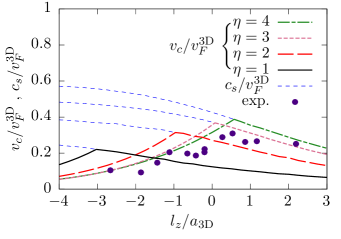
Figure 3: (color online). Landau critical velocity $v_{c}$ compared with the speed of sound $c_{s}$ across the BEC-BCS crossover, as a function of $l_{z}/a_{\text{3D}}$ at different values of $\eta$. The theoretical values at large $\eta$ may be compared with the experimental results of the critical velocity, obtained by Weimer et al. Weimer2015 for a 3D trapped Fermi gas with $\epsilon_{F}^{\text{3D}}/\hbar\omega_{z}\apprge 4.2$, which in our dimensional crossover units roughly corresponds to a dimension parameter $\eta=k_{F}^{\text{3D}}l_{z}^{\text{HO}}=\sqrt{\hbar\epsilon_{F}^{\text{3D}}/(M\omega_{z})}=2.9$. Here, $v_{F}^{\textrm{3D}}=\hbar k_{F}^{\textrm{3D}}/M$ is the 3D Fermi velocity.

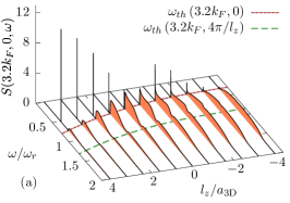
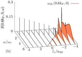
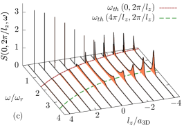
Figure 4: (color online). The density dynamic structure factor $S(\mathbf{Q}_{r},\omega)$ scaled by the ratio $\omega_{r}/N$, where $\omega_{r}$ is the recoil energy and $N$ the particle number, in the quasi-2D regime for $\eta=4$ at various interaction strengths $l_{z}/a_{\text{3D}}$, with the in-plane recoil momentum $\mathbf{Q}_{r}=(3.2k_{F},0)$ (a), $\mathbf{Q}_{r}=(0.6k_{F},0)$ (b) and transverse recoil momentum $\mathbf{Q}_{r}=(0,2\pi/l_{z})$ (c). The spectral width of the Bogoliubov-Anderson phonon peak is illustrated by the height of the delta function.

Landau critical velocity. — Within the GPF theory, we can calculate the critical velocity of the superfluid through both the BEC-BCS and dimensional crossover. Once we know the dispersion of in-plane ($q_{z}=0$) collective modes $\omega_{0}(q=\left|\mathbf{q}\right|)$, which corresponds to the poles of $[\mathbf{M}_{11}(Q)\mathbf{M}_{11}(-Q)-\mathbf{M}_{12}^{2}(Q)]^{-1}$, for a given set of the parameters $\eta$ and $l_{z}/a_{\text{3D}}$, we compute the speed of sound of the superfluid, $c_{s}=\lim_{q\rightarrow 0}\omega_{0}(q)/q$, and the pair-breaking velocity $v_{pb}=[\hbar^{2}(\sqrt{\Delta^{2}+\mu^{2}}-\mu)/M]^{1/2}$ Combescot2006 . According to Landau’s criterion, the critical velocity in the BEC-BCS crossover is then given by,

$$v_{c}=\min_{q\geq 0}\frac{\omega_{0}\left(q\right)}{q}=\min\left\{c_{s},v_{pb}\right\}.$$ (8)

In Fig. 3, we present the speeds of sound $c_{s}$ and critical velocities $v_{c}$ for dimensions $\eta=1\sim 4$ as a function of the interaction strength $l_{z}/a_{{\rm 3D}}$. The critical velocity of a 3D Fermi superfluid at the BEC-BCS crossover has been experimentally measured in a harmonic trap Miller2007 ; Weimer2015 and can be compared with our results using the transverse harmonic oscillator length, $l_{z}^{\text{HO}}=\sqrt{\hbar/(m\omega_{z})}$, as input to determine $\eta$. In Ref. Weimer2015 , the 3D regime is approximately reached with $\epsilon_{F}^{\text{3D}}/(\hbar\omega_{z})\apprge 4.2$ that corresponds to $\eta\simeq 2.9$ and the data match qualitatively well with the predicted Landau critical velocity (i.e., at $\eta=3$).

In 3D the BCS regime displays a large speed of sound and a smaller pair-breaking velocity that limits the critical velocity Combescot2006 ; Sensarma2006 . On the BEC side, close to the 3D unitarity, the pair-breaking velocity becomes equal to the speed of sound, which is referred to as the most robust configuration of the BEC-BCS crossover Combescot2006 . Beyond this point the speed of sound becomes the critical velocity, marking the system undergoing macroscopic condensation. The 2D and quasi-2D critical velocities behave similarly to the 3D case. However, the tuning point of the BEC-BCS crossover $(l_{z}/a_{\text{3D}})_{v_{c}^{\max}}$ – at which the critical velocity peaks – shows a non-trivial dependence on the dimensional parameter $\eta$. This enables us to characterize the dimensional crossover diagram in the presence of strong interactions, as shown in Fig. 1. In the region $0\leq\eta<2$, the 2D regime, we see the logarithmic dependence of the critical velocity maximum with respect to $\eta$, with the peak of the critical velocity in 2D at $\ln(k_{F}^{\text{2D}}a_{\text{2D}})\simeq 1.08$ footnote ; Shi2015 . Moreover, a linear behavior is observed in the nearly 3D regime with $\eta>8$ placing the peak of the critical velocity in 3D at $1/(k_{F}^{\text{3D}}a_{\text{3D}})\simeq 0.056$ footnote ; Combescot2006 . In between ($2<\eta<8,$), the maximum of the critical velocity lies in the interval $-1<l_{z}/a_{\text{3D}}<0.67$ and $(l_{z}/a_{\text{3D}})_{v_{c}^{\max}}$ varies non-monotonically with $\eta$. We identify this as the quasi-2D regime, consolidating the previous conclusion made from equation of state.

Probing the quasi-2D regime. — A practical way to measure both the speed of sound, $c_{s}$, and the order parameter, $\Delta$, is via Bragg spectroscopy. The spectroscopic response probes the dynamic structure factor Brunello2001 ; Veeravalli2008 ; Hoinka2013 , which in the case of a Fermi superfluid exhibits a peak corresponding to the Bogoliubov-Anderson phonon mode and a continuum of particle-hole excitations Combescot2006 . Due to the presence of a pairing gap in the excitation spectrum, an external excitation of momentum $\mathbf{Q}_{r}$ is collective if it does not break pairs when it excites states with energy below the threshold,

$$\omega_{\textrm{th}}(\mathbf{Q}_{r})=\left\{\begin{array}[]{cc}2\Delta&\textrm{$\mu>0$ and $\hbar^{2}\mathbf{Q}_{r}^{2}\leq 8M\mu$}\\ 2\sqrt{\mu_{\mathbf{Q}_{r}}^{2}+\Delta^{2}}&\textrm{otherwise}\end{array}\right.,$$ (9)

where $\mu_{\mathbf{Q}_{r}}=\mu-\hbar^{2}\mathbf{Q}_{r}^{2}/(2M)$, and for our dimensional crossover system with finite transverse periodic length $l_{z}$, we have set $\mathbf{Q}_{r}=(q_{r},q_{z})$, a combination of an in-plane momentum $q_{r}$, and a transverse excitation, $q_{z}=2\pi n_{z}/l_{z}$ for fixed integer $n_{z}$. We note that the calculation of the dynamic structure factor $S(\mathbf{Q}_{r},\omega)$ within the GPF theory is notoriously difficult He2016 , so we instead use the random phase approximation within the mean-field framework Zou2010 .

In Fig. 4, we plot the dynamic structure factor in the quasi-2D regime at $\eta=4$, normalized by the number of particles $N$ and recoil energy $\omega_{r}=\hbar\mathbf{Q}_{r}^{2}/(2M)$ for three different recoil momenta, (a) $\mathbf{Q}_{r}=(3.2k_{F},0)$, (b) $\mathbf{Q}_{r}=(0.6k_{F},0)$ and (c) $\mathbf{Q}_{r}=(0,2\pi/l_{z})$. One observes in Figs. 4(a)-(b) that the response is similar to the 3D case Zou2010 , showing the characteristic peaks in the continuum spectrum for $\omega>\omega_{\textrm{th}}$, and the presence of the phonon mode. We note the appearance of a second peak, marked by $\omega_{\textrm{th}}(q_{r},4\pi/l_{z})$ (green dashed) in Fig. 4(a), corresponding to the generation of a transverse excitation. The response at $\omega_{\textrm{th}}(q_{r},2\pi/l_{z})$ is absent, due to the need of the system to excite two modes along $z$ with opposite momenta, in order to conserve the total momentum. The same structure, present in Fig. 4(b), is not resolved due to the energy required at this momentum.

The dynamic response of the system, for a transverse recoil momentum $\mathbf{Q}_{r}=(0,2\pi/l_{z})$, is shown in Fig. 4(c), and has a specific structure due to the quasi-2D regime. Conservation of total momentum forces in-plane excitations to place the second continuum peak at $\omega_{\textrm{th}}(4\pi/l_{z},2\pi/l_{z})$ and gives no response at $\omega_{\textrm{th}}(2\pi/l_{z},2\pi/l_{z})$, which would break momentum conservation. We expect this to be a signature of the quasi-2D regime, as in 3D the pairing gap between box modes, $2\pi/l_{z}$, goes to zero and the isolated peaks merge in a continuous structure, while in 2D, the peak $\omega_{\textrm{th}}(4\pi/l_{z},2\pi/l_{z})$ moves too far away from the main spectrum.

Conclusions. — In summary, we have examined the role of dimension in a strongly interacting Fermi superfluid by treating the transverse confinement with PBC. We have mapped out a dimensional crossover diagram from the zero-temperature equation of state and have quantitatively determined the boundaries between 2D, quasi-2D, and 3D from the location of maximum Landau critical velocity. This sets a framework for characterizing the BCS-BEC crossover in quasi-2D, where the different regimes of the superfluid can be experimentally probed using Bragg spectroscopy. Our results are directly applicable to an interacting dimensional crossover Fermi gas realized by imposing a box trapping potential in the tight confinement direction Mukherjee2016 , and we expect our findings to be qualitatively similar under harmonic transverse confinement.

Supplemental Material for
“Dimensional crossover in a strongly interacting ultracold atomic Fermi gas”

Supplemental Material for
“Dimensional crossover in a strongly interacting ultracold atomic Fermi gas”

Umberto Toniolo

Brendan C. Mulkerin

Chris J. Vale

Xia-Ji Liu

Hui Hu

March 14, 2024

I Alternative characterizations of the dimensional crossover

The dimensional crossover is tuned by the quasi-2D BCS-BEC crossover parameter, $l_{z}/a_{\text{3D}}$, computed at the position where the Landau critical velocity has a maximum. Here, we present alternative chacterizations by using the ratio between the pairing order parameter $\Delta$ and the chemical potential $\mu$, or the ratio between the pairing order parameter and the Fermi energy $\varepsilon_{F}$.

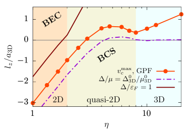
Figure S1: The evolution of the tuning parameter $l_{z}/a_{\text{3D}}$, computed at different conditions, as a function of the dimensional parameter $\eta$ (in logarithmic scale). $l_{z}/a_{\text{3D}}$ is computed (i) when the Landau critical velocity has a maximum (red line with circles), (ii) when the ratio between the order parameter $\Delta$ and the chemical potential $\mu$ reproduces the 3D typical values $\Delta_{\text{3D}}^{0}=0.46\varepsilon_{F}^{\text{3D}}$ and $\mu_{\text{3D}}^{0}=0.4\varepsilon_{F}^{\text{3D}}$ Hu2006 (purple dot-dashed line), and (iii) when $\Delta=\varepsilon_{F}$ (solid line at the top right).

In Fig. S1 we plot the critical values of $l_{z}/a_{\text{3D}}$, across the dimensional crossover, when, (i) the Landau critical velocity has a maximum (circles), (ii) the ratio $\Delta/\mu$ is equal to the 3D case (dashed-dotted) and (iii) when the order parameter, $\Delta$, is equal to the Fermi energy, $\varepsilon_{F}$. We observe that as expected, the ratio $\Delta/\mu$ approaches the 3D limit for $\eta\rightarrow\infty$, while the condition $\Delta=\varepsilon_{F}$ has meaning only in the far 2D limit. Indeed, the condition $\Delta=\varepsilon_{F}$ can be reached in 3D only at very large values of the tuning parameter $1/(k_{F}^{\text{3D}}a_{\text{3D}})$, in the deep BEC regime. We remark that the choice of the Landau critical velocity, as the most useful condition to characterize the crossover, allows a complete independent description from both the 3D and 2D regimes, since the interaction effect is fully taken into account in $v_{c}^{\max}$.

II Landau critical velocity in the 3D and 2D limits

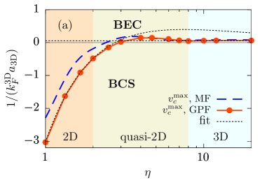
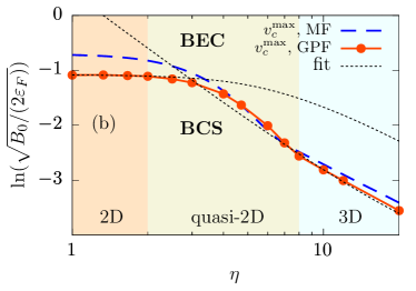
Figure S2: The dimensional crossover diagram tuned by the dimensional parameter, $\eta$, and (a) the typical 3D BCS-BEC crossover parameter, $1/(k_{F}^{\text{3D}}a_{\text{3D}})$, and (b) the typical 2D BCS-BEC crossover parameter, $\ln(\sqrt{B_{0}/(2\varepsilon_{F})})$. The fitted lines (tiny dotted) show (a) the expected constant behaviour $[1/(k_{F}^{\text{3D}}a_{\text{3D}})]_{v^{\max}_{c}}\simeq 0.056$ at $\eta\rightarrow\infty$, and (b) the expected constant behaviour $[\ln(\sqrt{B_{0}/(2\varepsilon_{F})})]_{v_{c}^{\max}}\simeq-1.08$ at $\eta\rightarrow 0$.

II.1 The 3D limit

We observe that, for a 3D Fermi gas, the MF theory predicts the critical velocity to be slightly on the BEC side at approximately $1/(k_{F}^{\text{3D}}a_{\text{3D}})_{v^{\max}_{c}}\simeq 0.07$ Combescot2006 . Figure 1 is expected to predict this behaviour when we restore the 3D limit case for $\eta\rightarrow\infty$. We consider the most general choice to descibe the BCS-BEC tuning parameter in this limit,

$$\left(\frac{l_{z}}{a_{\text{3D}}}\right)_{v_{c}^{\max}}=\sum_{n=-\infty}^{\infty}a_{n}\eta^{n}.$$ (S1)

The limit of the proper 3D tuning parameter, $1/(k_{F}^{\text{3D}}a_{\text{3D}})$, is then given by

$$\lim_{\eta\rightarrow\infty}\left(\frac{l_{z}}{a_{\text{3D}}}\right)_{v_{c}^{\max}}\frac{1}{\eta}=\sum_{n=-\infty}^{\infty}a_{n}\eta^{n-1}.$$ (S2)

Every coefficient $a_{n}$ for $n<1$ is negligible when $\eta$ is large enough, while each term $a_{n}\neq 0$, for $n>1$, would lead to a divergence in the definition of the 3D peak for the critical velocity and it is therefore discarded. We fit the far right hand side of Fig. 1 via a linear function,

$$\left(\frac{l_{z}}{a_{\text{3D}}}\right)_{v_{c}^{\max}}\Big{|}_{\eta\geq 8}=a_{0}+a_{1}\eta,$$ (S3)

and we included the $a_{0}$ term due to the proximity of data to the quasi-2D regime when $\eta\simeq 8$. This leads to

$$\left(\frac{1}{k_{F}^{\text{3D}}a_{\text{3D}}}\right)_{v^{\max}_{c}}=a_{1}\simeq 0.056.$$ (S4)

The behaviour in the 3D regime is shown in Fig. S2(a) that provides the same results of Fig. 1 with a change of scale in the vertical axis from $l_{z}/a_{\text{3D}}$ to $1/(k_{F}^{\text{3D}}a_{\text{3D}})$.

II.2 The 2D limit

In the 2D limit, we denote that

$$\left(\frac{l_{z}}{a_{\text{3D}}}\right)_{v_{c}^{\max}}=\mathcal{F}(\eta),$$ (S5)

where the approximate form of $\mathcal{F}(\eta)$ is to be determined. We observe from Fig. 2(a)-(b) that the proper BCS-BEC crossover tuning parameter becomes $\ln[\sqrt{B_{0}/(2\varepsilon_{F})}]$, where $k_{F}=k_{F}^{\text{2D}}$, for $\eta\leq\pi 6^{1/3}$, and $\lim_{\eta\rightarrow 0}\sqrt{B_{0}/(2\varepsilon_{F})}=1/(k_{F}^{\text{2D}}a_{\text{2D}})$. We consider the relation between the 2D and the quasi-2D tuning parameters,

$$\sqrt{\frac{B_{0}}{2\epsilon_{F}}}=\frac{\sqrt{3\pi}}{\eta^{3/2}}\text{arcsinh}\left[\frac{1}{2}\exp\left(\frac{l_{z}}{2a_{\text{3D}}}\right)\right].$$ (S6)

It is reasonable to assume that at the position where the Landau critical velocity takes the maximum value, we would have,

$$\lim_{\eta\rightarrow 0}\sqrt{\frac{B_{0}}{2\epsilon_{F}}}=A\neq 0.$$ (S7)

By using the above three equations, we find that,

$$\mathcal{F}(\eta)=2\ln\left[\sinh\left(\frac{A\eta^{3/2}}{\sqrt{3\pi}}\right)\right]\sim_{\eta=0}2\ln\left(\frac{2A}{\sqrt{3\pi}}\right)+3\ln\eta+\mathcal{O}(\eta^{3}).$$ (S8)

Therefore, our numerical results in the 2D limit could be fitted with the function

$$\mathcal{F}(\eta)=W+Z\ln{\eta}.$$ (S9)

We obtain the values $W=3.02$ and $Z=2.97$ from the fitting. The latter value $Z\simeq 3$ confirms our theoretical anticipation of the 2D limit, within a relative error of a few percents. Using the former value of $W$, we can compute the position of the Landau critical velocity peak in the 2D limit being,

$$\lim_{\eta\rightarrow 0}\ln\left(\sqrt{\frac{B_{0}}{2\epsilon_{F}}}\right)_{v_{c}^{\max}}=\ln A=\frac{W}{2}+\ln\frac{\sqrt{3\pi}}{2}\simeq-1.08,$$ (S10)

as represented in the dimensional crossover diagram of Fig. S2(b) that provides the same results of Fig. 1 with a change of scale in the vertical axis from $l_{z}/a_{\text{3D}}$ to $\ln[\sqrt{B_{0}/(2\varepsilon_{F})}]$. This extracted position of the peak of the Landau critical velocity in the 2D limit is consistent with the position of the peak of the contact, $\ln(k_{F}^{2D}a_{2D})\sim 1$, obtained recently via auxiliary-field Monte Carlo simulations for a 2D interacting Fermi gas Shi2015 .