On the Local Structure of Stable Clustering Instances

Abstract

We study the classic $k$-median and $k$-means clustering objectives in the beyond-worst-case scenario. We consider three well-studied notions of structured data that aim at characterizing real-world inputs:

• Distribution Stability (introduced by Awasthi, Blum, and Sheffet, FOCS 2010)

• Spectral Separability (introduced by Kumar and Kannan, FOCS 2010)

• Perturbation Resilience (introduced by Bilu and Linial, ICS 2010)

We prove structural results showing that inputs satisfying at least one of the conditions are inherently “local”. Namely, for any such input, any local optimum is close both in term of structure and in term of objective value to the global optima.

As a corollary we obtain that the widely-used Local Search algorithm has strong performance guarantees for both the tasks of recovering the underlying optimal clustering and obtaining a clustering of small cost. This is a significant step toward understanding the success of local search heuristics in clustering applications.

1 Introduction

Clustering is a fundamental, routinely-used approach to extract information from datasets. Given a dataset and the most important features of the data, a clustering is a partition of the data such that data elements in the same part have common features. The problem of computing a clustering has received a considerable amount of attention in both practice and theory.

The variety of contexts in which clustering problems arise makes the problem of computing a “good” clustering hard to define formally. From a theoretician’s perspective, clustering problems are often modeled by an objective function we wish to optimize (e.g., the famous $k$-median or $k$-means objective functions). This modeling step is both needed and crucial since it provides a framework to quantitatively compare algorithms. Unfortunately, the most popular objectives for clustering, like the $k$-median and $k$-means objectives, are hard to approximate, even when restricted to Euclidean spaces.

This view is generally not shared by practitioners. Indeed, clustering is often used as a preprocessing step to simplify and speed up subsequent analysis, even if this analysis admits polynomial time algorithms. If the clustering itself is of independent interest, there are many heuristics with good running times and results on real-world inputs.

This induces a gap between theory and practice. On the one hand, the algorithms that are efficient in practice cannot be proven to achieve good approximation to the $k$-median and $k$-means objectives in the worst-case. Since approximation ratios are one of the main methods to evaluate algorithms, theory predicts that determining a good clustering is a difficult task. On the other hand, the best theoretical algorithms turn out to be noncompetitive in applications because they are designed to handle “unrealistically” hard instances with little importance for practitioners. To bridge the gap between theory and practice, it is necessary to go beyond the worst-case analysis by, for example, characterizing and focusing on inputs that arise in practice.

1.1 Real-world Inputs

Several approaches have been proposed to bridge the gap between theory and practice. For example, researchers have considered the average-case scenario (e.g., [26]) where the running time of an algorithm is analyzed with respect to some probability distribution over the set of all inputs. Smooth analysis (e.g., [90]) is another celebrated approach that analyzes the running time of an algorithm with respect to worst-case inputs subject to small random perturbations.

Another successful approach, the one we take in this paper, consists in focusing on structured inputs. In a seminal paper, Ostrovsky, Rabani, Schulman, and Swamy [85] introduced the idea that inputs that come from practice induce a ground-truth or a meaningful clustering. They argued that an input $I$ contains a meaningful clustering into $k$ clusters if the optimal $k$-median cost of a clustering using $k$ centers, say $\text{OPT}_{k}(I)$, is much smaller than the optimal cost of a clustering using $k-1$ centers $\text{OPT}_{k-1}(I)$. This is also motivated by the elbow method (see Section 7 for more details) used by practitioners to define the number of clusters. More formally, an instance $I$ of $k$-median or $k$-means satisfies the $\alpha$-ORSS property if $\text{OPT}_{k}(I)/\text{OPT}_{k-1}(I)\leq\alpha$.

$\alpha$-ORSS inputs exhibit interesting properties. The popular $k$-means$++$ algorithm (also known as the $D^{2}$-sampling technique) achieves an $O(1)$-approximation for these inputs. The condition is also robust with respect to noisy perturbations of the data set. ORSS-stability also implies several other conditions aiming to capture well-clusterable instances. Thus, the inputs satisfying the ORSS property arguably share some properties with the real-world inputs. In this paper, we also provide experimental results supporting this claim, see Appendix C.

These results have opened new research directions and raised several questions. For example:

• Is it possible to obtain similar results for more general classes of inputs?

• How does the parameter $\alpha$ impact the approximation guarantee and running time?

• Is it possible to prove good performance guarantees for other popular heuristics?

• How close to the “ground-truth” clustering are the approximate clusterings?

We now review the most relevant work in connection to the above open questions, see Sections 2 for other related work.

Distribution Stability (Def. 4.1)

Awasthi, Blum and Sheffet [12] have tackled the first two questions by introducing the notion of distribution stable instances. Distribution stable instances are a generalization of the ORSS instances (in other words, any instance satisfying the ORSS property is distribution stable). They also introduced a new algorithm tailored for distribution stable instances that achieves a $(1+\varepsilon)$-approximation for $\alpha$-ORSS inputs (and more generally $\alpha$-distribution stable instances) in time $n^{O(1/\varepsilon\alpha)}$. This was the first algorithm whose approximation guarantee was independent from the parameter $\alpha$ for $\alpha$-ORSS inputs.

Spectral Separability (Def. 6.1)

Kumar and Kannan [74] tackled the first and third questions by introducing the proximity condition. This condition also generalizes the ORSS condition. It is motivated by the goal of learning a distribution mixture in a $d$-dimensional Euclidean space. Quoting [74], the message of their paper can loosely be stated as:

If the projection of any data point onto the line joining its cluster center to any other cluster center is $\gamma k$ times standard deviations closer to its own center than the other center, then we can cluster correctly in polynomial time.

In addition, they have made a significant step toward understanding the success of the classic $k$-means by showing that it achieves a $1+O(1/\gamma)$-approximation for instances that satisfy the proximity condition.

Perturbation Resilience (Def. 5.1)

In a seminal work, Bilu and Linial [29] introduced a new condition to capture real-world instances. They argue that the optimal solution of a real-world instance is often much better than any other solution and so, a slight perturbation of the instance does not lead to a different optimal solution. Perturbation-resilient instances have been studied in various contexts (see e.g.,  [13, 16, 20, 21, 27, 76]). For clustering problems, an instance is said to be $\alpha$-perturbation resilient if an adversary can change the distances between pairs of elements by a factor at most $\alpha$ and the optimal solution remains the same. Recently, Angelidakis, Makarychev, and Makarychev [80] have given a polynomial-time algorithm for solving $2$-perturbation-resilient instances. Balcan and Liang [21] have tackled the third question by showing that a classic algorithm for hierarchical clustering can solve $1+\sqrt{2}$-perturbation-resilient instances. This very interesting result leaves open the question as whether classic algorithms for (“flat”) clustering could also be proven to be efficient for perturbation-resilient instances.

Main Open Questions

Previous work has made important steps toward bridging the gap between theory and practice for clustering problems. However, we still do not have a complete understanding of the properties of “well-structured” inputs, nor do we know why the algorithms used in practice perform so well. Some of the most important open questions are the following:

• Do the different definitions of well-structured input have common properties?

• Do heuristics used in practice have strong approximation ratios for well-structured inputs?

• Do heuristics used in practice recover the “ground-truth” clustering on well-structured inputs?

1.2 Our Results: A unified approach via Local Search

We make a significant step toward answering the above open questions. We show that the classic Local Search heuristic (see Algorithm 1), that has found widespread application in practice (see Section 2), achieves good approximation guarantees for distribution-stable, spectrally-separable, and perturbation-resilient instances (see Theorems 4.2, 5.2, 6.2).

More concretely, we show that Local Search is a polynomial-time approximation scheme (PTAS) for both distribution-stable and spectrally-separable instances. In the case of distribution stability, we also answer the above open question by showing that most of the structure of the optimal underlying clustering is recovered by the algorithm. Furthermore, our results hold even when only a $\delta$ fraction (for any constant $\delta>0$) of the points of each optimal cluster satisfies the $\beta$-distribution-stability property.

For $\gamma$-perturbation-resilient instances, we show that if $\gamma>3$ then any solution is the optimal solution if it cannot be improved by adding or removing $2\gamma$ centers. We also show that the analysis is essentially tight.

These results show that well-structured inputs have the property that the local optima are close both qualitatively (in terms of structure) and quantitatively (in terms of objective value) to the global “ground-truth” optimum. These results make a significant step toward explaining the success of Local Search approaches for solving clustering problems in practice.

Algorithm 1 Local Search($\varepsilon$) for $k$-Median and $k$-Means

1:Input: $A,F,\text{cost},k$

2:Parameter: $\varepsilon$

3:$S\leftarrow$ Arbitrary subset of $F$ of cardinality at most $k$.

4:while $\exists$ $S^{\prime}$ s.t. $|S^{\prime}|\leq k$ and $|S-S^{\prime}|+|S^{\prime}-S|\leq 2/\varepsilon$ and cost($S^{\prime}$) $\leq$ $(1-\varepsilon/n)$ cost($S$)

5: do

6:     $S\leftarrow S^{\prime}$

7:end while

8:Output: $S$

1.3 Organization of the Paper

Section 2 provides a more detailed review of previous work on worst-case approximation algorithms and Local Search. Further comments on stability conditions not covered in the introduction can be found in Section 7 at the end of the paper. Section 3 introduces preliminaries and notation. Section 4 is dedicated to distribution-stable instances, Section 5 to perturbation-resilient instances, and Section 6 to spectrally-separated instances. All the missing proofs can be found in the appendix.

2 Related Work

Worst-Case Hardness

The problems we study are NP-hard: $k$-median and $k$-means are already NP-hard in the Euclidean plane (see Meggido and Supowit [83], Mahajan et al.  [79], and Dasgupta and Freud [43]). In terms of hardness of approximation, both problems are APX-hard, even in the Euclidean setting when both $k$ and $d$ are part of the input (see Guha and Khuller [56], Jain et al. [64], Guruswami et al. [59], and Awasthi et al. [14]). On the positive side, constant factor approximations are known in metric space for both $k$-median and $k$-means (see [3, 33, 77, 65, 84]). For Euclidean spaces we have a PTAS for both problems, either assuming $d$ fixed and $k$ arbitrary [7, 37, 52, 62, 63, 72], or assuming $k$ fixed and $d$ arbitrary [48, 75].

Local Search

Local Search is an all-purpose heuristic that may be applied to any problem, see Aarts and Lenstra [1] for a general introduction. For clustering, there exists a large body of bicriteria approximations for $k$-median and $k$-means [23, 34, 38, 73]. Arya et al. [11] showed that Local Search with a neighborhood size of $1/\varepsilon$ gives a $3+2\varepsilon$ approximation to $k$-median, see also [58]. Kanungo et al. [70] proved an approximation ratio of $9+\varepsilon$ for $k$-means clustering by Local Search, which was until very recently [3] the best known algorithm with a polynomial running time in metric and Euclidean spaces. Recently, Local Search with an appropriate neighborhood size was shown to be a PTAS for $k$-means and $k$-median in certain restricted metrics including constant dimensional Euclidean space [37, 52]. Due to its simplicity, Local Search is also a popular subroutine for clustering tasks in various more specialized computational models [24, 30, 57]. For more theoretical clustering papers using Local Search, we refer to [39, 45, 53, 60, 95].

Local Search is also often used for clustering in more applied areas of computer science (e.g., [92, 54, 4, 61]). Indeed, the use of Local Search with a neighborhood of size $1$ for clustering was first proposed by Tüzün and Burke [93], see also Ghosh [55] for a more efficient version of the same approach. Due the ease by which it may be implemented, Local Search has become one of the most commonly used heuristics for clustering and facility location, see Ardjmand [5]. Nevertheless, high running times is one of the biggest drawbacks of Local Search compared to other approaches, though a number of papers have engineered it to become surprisingly competitive, see Frahling and Sohler [51], Kanungo et al. [69], and Sun [91].

3 Definitions and Notations

The problem

The problem we consider in this work is the following slightly more general version of the $k$-means and $k$-median problems.

Definition 3.1 ($k$-Clustering).

Let $A$ be a set of clients, $F$ a set of centers, both lying in a metric space $(\mathcal{X},\text{dist})$, cost a function $A\times F\rightarrow\mathbb{R}_{+}$, and $k$ a non-negative integer. The $k$-clustering problem asks for a subset $S$ of $F$, of cardinality at most $k$, that minimizes

$$\text{cost}(S)=\sum_{x\in A}\min_{c\in S}\text{cost}(x,c).$$

The clustering of $A$ induced by $S$ is the partition of $A$ into subsets $C=\{C_{1},\ldots C_{k}\}$ such that $C_{i}=\{x\in A~{}|~{}c_{i}=\underset{c\in S}{\text{argmin }}\text{cost}(x,c)\}$ (breaking ties arbitrarily).

The well known $k$-median and $k$-means problems correspond to the special cases $\text{cost}(a,c)=\text{dist}(a,c)$ and $\text{cost}(a,c)=\text{dist}(a,c)^{2}$ respectively. Throughout the rest of this paper, let OPT denote the value of an optimal solution. To give slightly simpler proofs for $\beta$-distribution-stable and $\alpha$-perturbation-resilient instances, we will assume that $\text{cost}(a,b)=\text{dist}(a,b)$. If $\text{cost}(a,b)=\text{dist}(a,b)^{p}$, then $\alpha$ depends exponentially on the $p$ for perturbation resilience. For distribution stability, we still have a PTAS by introducing a dependency in $1/\varepsilon^{O(p)}$ in the neighborhood size of the algorithm. The analysis is unchanged save for various applications of the following lemma at different steps of the proof.

Lemma 3.2.

Let $p\geq 0$ and $1/2>\varepsilon>0$. For any $a,b,c\in A\cup F$, we have $\text{cost}(a,b)\leq(1+\varepsilon)^{p}\text{cost}(a,c)+\text{cost}(c,b)(1+1/\varepsilon)^{p}$.

4 Distribution Stability

We work with the notion of $\beta,\delta$-distribution stability which generalizes $\beta$-distribution stability. This extends our result to datasets that exhibit a slightly weaker structure than the $\beta$-distribution stability. Namely, the $\beta,\delta$-distribution stability only requires that for each cluster of the optimal solution, most of the points satisfy the $\beta$-distribution stability condition.

Figure 1: Example of a cluster $C^{*}_{i}\not\in Z^{*}$. An important fraction of the points in $\text{IR}^{\varepsilon^{2}}_{i}$ are served by $\mathcal{L}(i)$ and few points in $\bigcup_{j\neq i}\Delta_{j}$ are served by $\mathcal{L}(i)$.

Definition 4.1 ($(\beta,\delta)$-Distribution Stability).

Let $(A,F,\text{cost},k)$ be an instance of $k$-clustering where $A\cup F$ lie in a metric space and let $S^{*}=\{c^{*}_{1},\ldots,c^{*}_{k}\}\subseteq F$ be a set of centers and $C^{*}=\{C^{*}_{1},\ldots,C^{*}_{k}\}$ be the clustering induced by $S^{*}$. Further, let $\beta>0$ and $0\leq\delta\leq 1$. Then the pair $(A,F,\text{cost},k),(C^{*},S^{*})$ is a $(\beta,\delta)$-distribution stable instance if, for any $i$, there exists a set $\Delta_{i}\subseteq C^{*}_{i}$ such that $|\Delta_{i}|\geq(1-\delta)|C^{*}_{i}|$ and for any $x\in\Delta_{i}$, for any $j\neq i$,

$$\text{cost}(x,c^{*}_{j})\geq\beta\frac{\text{OPT}}{|C^{*}_{j}|},$$

where $\text{cost}(x,c^{*}_{j})$ is the cost of assigning $x$ to $c^{*}_{j}$.

For any instance $(A,F,\text{cost},k)$ that is $(\beta,\delta)$-distribution stable, we refer to $(C^{*},S^{*})$ as a $(\beta,\delta)$-clustering of the instance. We show the following theorem for the $k$-median problem. For the $k$-clustering problem with parameter $p$, the constant $\eta$ becomes a function of $p$.

Theorem 4.2.

Let $p>0$, $\beta>0$, and $\varepsilon<\min(1-\delta,1/3)$. For a $(\beta,\delta)$-stable instance with $(\beta,\delta)$ clustering $(C^{*},S^{*})$ and an absolute constant $\eta$, the cost of the solution output by Local Search$(4\varepsilon^{-3}\beta^{-1}+O(\varepsilon^{-2}\beta^{-1}))$ (Algorithm 1) is at most $(1+\eta\varepsilon)\text{cost}(C^{*})$.

Moreover, let $L=\{L_{1},\ldots,L_{k}\}$ denote the clusters of the solution output by Local Search$(4\varepsilon^{-3}\beta^{-1}+O(\varepsilon^{-2}\beta^{-1}))$. If $\delta=0$ (i.e.: the instance is simply $\beta$-distribution-stable), there exists a bijection $\phi:L\mapsto C^{*}$ such that for at least $m=k-O(\varepsilon^{-3}\beta^{-1})$ clusters $L^{\prime}_{1},\ldots,L^{\prime}_{m}\subseteq L$, the following two statements hold.

• At least a $(1-\varepsilon)$ fraction of $\text{IR}^{\varepsilon^{2}}_{i}\cap C^{*}_{i}$ are served by a unique center $\mathcal{L}(i)$ in solution $\mathcal{L}$.

• The total number of clients $p\in\bigcup_{j\neq i}C^{*}_{j}$ served by $\mathcal{L}(i)$ in $\mathcal{L}$ is at most $\varepsilon|\text{IR}^{\varepsilon^{2}}_{i}\cap C^{*}_{i}|$.

We first give a high-level description of the analysis. Assume for simplicity that all the optimal clusters cost less than an $\varepsilon^{3}$ fraction of the total cost of the optimal solution. Combining this assumption with the $\beta$-distribution-stability property, one can show that the centers and points close to the center are far away from each other. Thus, guided by the objective function, the local search algorithm identifies most of these centers. In addition, we can show that for most of these good centers the corresponding cluster in the local solution is very similar to the optimal cluster (see Figure 1). In total, only very few clusters (a function of $\varepsilon$ and $\beta$) of the optimal solution are not present in the local solution. We conclude our proof by using local optimality. Our proof includes a few ingredients from [12] such as the notion of inner-ring (we work with a slightly more general definition) and distinguishes between cheap and expensive clusters. Nevertheless our analysis is slightly stronger as we consider a significantly weaker stability condition and can not only analyze the cost of the solution of the algorithm, but also the structure of its clusters.

Throughout this section, we consider a set of centers $S^{*}=\{c^{*}_{1},\ldots,c^{*}_{k}\}$ whose induced clustering is $C^{*}=\{C^{*}_{1},\ldots,C^{*}_{k}\}$ and such that the instance is $(\beta,\delta)$-stable with respect $(C^{*},S^{*})$. We denote by clusters the parts of a partition $C^{*}=\{C^{*}_{1},\ldots,C^{*}_{k}\}$. Let $\text{cost}(C^{*})=\sum_{i=1}^{k}\sum_{x\in C^{*}_{i}}\text{cost}(x,c^{*}_{i})$. Moreover, for any cluster $C^{*}_{i}$, for any client $x\in C^{*}_{i}$, denote by $g_{x}$ the cost of client $x$ in solution $C^{*}$: $g_{x}=\text{cost}(x,c^{*}_{i})=\text{dist}(x,c^{*}_{i})$ since we consider the $k$-median problem. Let $\mathcal{L}$ denote the output of LocalSearch($\beta^{-1}\varepsilon^{-3}$) and $l_{x}$ the cost induced by client $x$ in solution $\mathcal{L}$, namely $l_{x}=\min_{\ell\in\mathcal{L}}\text{cost}(x,\ell)$, and $\text{cost}(\mathcal{L})=\sum_{x\in A}l_{x}$. The following definition is a generalization of the inner-ring definition of [12].

Definition 4.3.

For any $\varepsilon_{0}$, we define the inner ring of cluster $i$, $\text{IR}^{\varepsilon_{0}}_{i}$, as the set of $x\in A\cup F$ such that $\text{dist}(x,c^{*}_{i})\leq\varepsilon_{0}\beta{\text{OPT}}/{|C^{*}_{i}|}$.

We say that cluster $i$ is cheap if $\sum_{x\in C^{*}_{i}}g_{x}\leq\varepsilon^{3}\beta\text{OPT}$, and expensive otherwise. We aim at proving the following structural lemma.

Lemma 4.4.

There exists a set of clusters $Z^{*}\subseteq C^{*}$ of size at most $2\varepsilon^{-3}\beta^{-1}+O(\varepsilon^{-2}\beta^{-1})$ such that for any cluster $C^{*}_{i}\in C^{*}-Z^{*}$, we have the following properties

1. $C^{*}_{i}$ is cheap.

2. At least a $(1-\varepsilon)$ fraction of $\text{IR}^{\varepsilon^{2}}_{i}\cap C^{*}_{i}$ are served by a unique center $\mathcal{L}(i)$ in solution $\mathcal{L}$.

3. The total number of clients $p\in\bigcup_{j\neq i}\Delta_{j}$ served by $\mathcal{L}(i)$ in $\mathcal{L}$ is at most $\varepsilon|\text{IR}^{\varepsilon^{2}}_{i}\cap C^{*}_{i}|$.

See Fig 1 for a typical cluster of $C^{*}-Z^{*}$. We start with the following lemma which generalizes Fact 4.1 in [12].

Lemma 4.5.

Let $C^{*}_{i}$ be a cheap cluster. For any $\varepsilon_{0}$, we have $|\text{IR}^{\varepsilon_{0}}_{i}\cap C_{i}^{*}|>(1-{\varepsilon^{3}}/{\varepsilon_{0}})|C^{*}_{i}|$.

We then prove that the inner rings of cheap clusters are disjoint for $\delta+\frac{\varepsilon^{3}}{\varepsilon_{0}}<1$ and $\varepsilon_{0}<\frac{1}{3}$.

Lemma 4.6.

Let $\delta+\frac{\varepsilon^{3}}{\varepsilon_{0}}<1$ and $\varepsilon_{0}<\frac{1}{3}$. If $C^{*}_{i}\neq C^{*}_{j}$ are cheap clusters, then $\text{IR}^{\varepsilon_{0}}_{i}\cap\text{IR}^{\varepsilon_{0}}_{j}=\emptyset$.

For each cheap cluster $C^{*}_{i}$, let $\mathcal{L}(i)$ denote a center of $\mathcal{L}$ that belongs to $\text{IR}^{\varepsilon}_{i}$ if there exists exactly such center and remain undefined otherwise. By Lemma 4.6, $\mathcal{L}(i)\neq\mathcal{L}(j)$ for $i\neq j$.

Lemma 4.7.

Let $\varepsilon<\frac{1}{3}$. Let $C^{*}-Z_{1}$ denote the set of clusters $C^{*}_{i}$ that are cheap, such that $\mathcal{L}(i)$ is defined and such that at least $(1-\varepsilon)|\text{IR}^{\varepsilon^{2}}_{i}\cap C_{i}^{*}|$ clients of $\text{IR}^{\varepsilon^{2}}_{i}\cap C_{i}^{*}$ are served in $\mathcal{L}$ by $\mathcal{L}(i)$. Then $|Z_{1}|\leq(2\varepsilon^{-3}+11.25\cdot\varepsilon^{-2}+22.5\cdot\varepsilon^{-1})\beta^{-1}$.

Proof.

There are five different types of clusters in $C^{*}$:

1. $k_{1}$ expensive clusters

2. $k_{2}$ cheap clusters with no center of $\mathcal{L}$ belonging to $\text{IR}^{\varepsilon}_{i}$

3. $k_{3}$ cheap clusters with at least two centers of $\mathcal{L}$ belonging to $\text{IR}^{\varepsilon}_{i}$

4. $k_{4}$ cheap clusters with $\mathcal{L}(i)$ being defined and less than $(1-\varepsilon)|\text{IR}^{\varepsilon^{2}}_{i}\cap C_{i}^{*}|$ clients of $\text{IR}^{\varepsilon^{2}}_{i}\cap C_{i}^{*}$ are served in $\mathcal{L}$ by $\mathcal{L}(i)$

5. $k_{5}$ cheap clusters with $\mathcal{L}(i)$ being defined and at least $(1-\varepsilon)|\text{IR}^{\varepsilon^{2}}_{i}\cap C_{i}^{*}|$ clients of $\text{IR}^{\varepsilon^{2}}_{i}\cap C_{i}^{*}$ are served in $\mathcal{L}$ by $\mathcal{L}(i)$

The definition of cheap clusters immediately yields $k_{1}\leq\varepsilon^{-3}\beta^{-1}$.

Since $\mathcal{L}$ and $C^{*}$ both have $k$ clusters and the inner rings of cheap clusters are disjoint (Lemma 4.6), we have $c_{1}k_{1}+c_{3}k_{3}+k_{4}+k_{5}=k_{1}+k_{2}+k_{3}+k_{4}+k_{5}=|Z_{1}|+k_{5}=k$ with $c_{1}\geq 0$ and $c_{3}\geq 2$ resulting in $k_{3}\leq(c_{3}-1)k_{3}=(1-c_{1})k_{1}+k_{2}\leq k_{1}+k_{2}$.

Before bounding $k_{2}$ and $k_{4}$, we discuss the impact of a cheap cluster $C^{*}_{i}$ with at least a $p$ fraction of the clients of $\text{IR}^{\varepsilon^{2}}_{i}\cap C_{i}^{*}$ being served in $\mathcal{L}$ by some centers that are not in $\text{IR}^{\varepsilon}_{i}$. By the triangular inequality, the cost for any client $x$ of this $p$ fraction is at least $(\varepsilon-\varepsilon^{2})\beta\text{cost}(C^{*})/|C^{*}_{i}|$. Then the total cost of all clients of this $p$ fraction in $\mathcal{L}$ is at least $p|\text{IR}^{\varepsilon^{2}}_{i}\cap C_{i}^{*}|(1-\varepsilon)\varepsilon\beta\text{cost}(C^{*})/|C^{*}_{i}|$. By Lemma 4.5, substituting $|\text{IR}^{\varepsilon^{2}}_{i}\cap C^{*}_{i}|$ yields for this total cost

$$p|\text{IR}^{\varepsilon^{2}}_{i}\cap C_{i}^{*}|(1-\varepsilon)\varepsilon\beta\frac{\text{cost}(C^{*})}{|C^{*}_{i}|}\geq p(1-\varepsilon)^{2}|C^{*}_{i}|\varepsilon\beta\frac{\text{cost}(C^{*})}{|C^{*}_{i}|}=p(1-\varepsilon)^{2}\varepsilon\beta\text{cost}(C^{*}).$$

To determine $k_{2}$, we must use $p=1$ while we have $p>\varepsilon$ for $k_{4}$. Therefore, the total costs of all clients of the $k_{2}$ and the $k_{4}$ clusters in $\mathcal{L}$ are at least $k_{2}(1-\varepsilon)^{2}\varepsilon\beta\text{cost}(C^{*})$ and $k_{4}(1-\varepsilon)^{2}\varepsilon^{2}\beta\text{cost}(C^{*})$, respectively.

Now, since $\text{cost}(\mathcal{L})\leq 5\text{OPT}\leq 5\text{cost}(C^{*})$, we have $(k_{2}+k_{4}\varepsilon)\varepsilon\beta\leq 5/(1-\varepsilon)^{2}\leq 45/4$.

Therefore, we have $|Z_{1}|=k_{1}+k_{2}+k_{3}+k_{4}\leq 2k_{1}+2k_{2}+k_{4}\leq(2\varepsilon^{-3}+11.25\cdot\varepsilon^{-2}+22.5\cdot\varepsilon^{-1})\beta^{-1}$. ∎

We continue with the following lemma, whose proof relies on similar arguments.

Lemma 4.8.

There exists a set $Z_{2}\subseteq C^{*}-Z_{1}$ of size at most $11.25\varepsilon^{-1}\beta^{-1}$ such that for any cluster $C^{*}_{j}\in C^{*}-Z_{2}$, the total number of clients $x\in\bigcup_{i\neq j}\Delta_{i}$, that are served by $\mathcal{L}(j)$ in $\mathcal{L}$ is at most $\varepsilon|\text{IR}^{\varepsilon^{2}}_{i}\cap C_{i}^{*}|$.

Therefore, the proof of Lemma 4.4 follows from combining Lemmas 4.7 and 4.8.

We now turn to the analysis of the cost of $\mathcal{L}$. Let $C(Z^{*})=\bigcup_{C^{*}_{i}\in Z^{*}}C^{*}_{i}$. For any cluster $C^{*}_{i}\in C^{*}-Z^{*}$, let $\mathcal{L}(i)$ be the unique center of $\mathcal{L}$ that serves at least $(1-\varepsilon)|\text{IR}^{\varepsilon^{2}}_{i}\cap C_{i}^{*}|>(1-\varepsilon)^{2}|C_{i}|$ clients of $\text{IR}^{\varepsilon^{2}}_{i}\cap C^{*}_{i}$, see Lemmas 4.4 and 4.5. Let $\widehat{\mathcal{L}}=\bigcup_{C^{*}_{i}\in C^{*}-Z^{*}}\mathcal{L}(i)$ and define $\widehat{A}$ to be the set of clients that are served in solution $\mathcal{L}$ by centers of $\widehat{\mathcal{L}}$. Finally, let $A(\mathcal{L}(i))$ be the set of clients that are served by $\mathcal{L}(i)$ in solution $\mathcal{L}$. Observe that the $A(\mathcal{L}(i))$ partition $\widehat{A}$.

Lemma 4.9.

We have

$$-{\varepsilon}\cdot\text{cost}(\mathcal{L})/n+\sum\limits_{x\in\widehat{A}-C(Z^{*})}l_{x}\leq\sum\limits_{x\in\widehat{A}-C(Z^{*})}g_{x}+\frac{2\varepsilon}{(1-\varepsilon)^{2}}\cdot(\text{cost}(C^{*})+\text{cost}(\mathcal{L})).$$

Proof.

Consider the following mixed solution $\mathcal{M}=\widehat{\mathcal{L}}\cup\{c_{i}^{*}~{}|~{}C_{i}^{*}\in Z^{*}\}$. We start by bounding the cost of $\mathcal{M}$. For any client $x\in\widehat{A}$, the center that serves it in $\mathcal{L}$ belongs to $\mathcal{M}$. Thus its cost in $\mathcal{M}$ is at most $l_{x}$. Now, for any client $x\in C(Z^{*})$, the center that serves it in $C^{*}$ is in $\mathcal{M}$, so its cost in $\mathcal{M}$ is at most $g_{x}$.

Finally, we evaluate the cost of the clients in $A-(\widehat{A}\cup C(Z^{*}))$. Consider such a client $x$ and let $C^{*}_{i}$ be the cluster it belongs to in solution $C^{*}$. Since $C^{*}_{i}\in C^{*}-Z^{*}$, $\mathcal{L}(i)$ is defined and we have $\mathcal{L}(i)\in\widehat{\mathcal{L}}\subseteq\mathcal{M}$. Hence, the cost of $x$ in $\mathcal{M}$ is at most $\text{cost}(x,\mathcal{L}(i))$. Observe that by the triangular inequality, $\text{cost}(x,\mathcal{L}(i))\leq\text{cost}(x,c^{*}_{i})+\text{cost}(c^{*}_{i},\mathcal{L}(i))=g_{x}+\text{cost}(c^{*}_{i},\mathcal{L}(i))$.

Now consider a client $x^{\prime}\in\text{IR}_{i}^{\varepsilon^{2}}\cap C^{*}_{i}\cap A(\mathcal{L}(i))$. By the triangular inequality, we have $\text{cost}(c^{*}_{i},\mathcal{L}(i))\leq\text{cost}(c^{*}_{i},x^{\prime})+\text{cost}(x^{\prime},\mathcal{L}(i))=g_{x^{\prime}}+l_{x^{\prime}}$. Hence,

$$\text{cost}(c^{*}_{i},\mathcal{L}(i))\leq\frac{1}{|\text{IR}_{i}^{\varepsilon^{2}}\cap C^{*}_{i}\cap A(\mathcal{L}(i))|}\sum\limits_{x^{\prime}\in\text{IR}_{i}^{\varepsilon^{2}}\cap C^{*}_{i}\cap A(\mathcal{L}(i))}(g_{x^{\prime}}+l_{x^{\prime}}).$$

It follows that assigning the clients of $C^{*}_{i}\cap(A-\widehat{A})$ to $\mathcal{L}(i)$ induces a cost of at most

$$\sum\limits_{x\in C^{*}_{i}\cap(A-\widehat{A})}g_{x}+\frac{|C^{*}_{i}\cap(A-\widehat{A})|}{|\text{IR}_{i}^{\varepsilon^{2}}\cap C^{*}_{i}\cap A(\mathcal{L}(i))|}\sum\limits_{x^{\prime}\in\text{IR}_{i}^{\varepsilon^{2}}\cap C^{*}_{i}\cap A(\mathcal{L}(i))}(g_{x^{\prime}}+l_{x^{\prime}}).$$

Due to Lemma 4.4, we have $|\text{IR}_{i}^{\varepsilon^{2}}\cap C^{*}_{i}\cap A(\mathcal{L}(i))|\geq(1-\varepsilon)\cdot|\text{IR}_{i}^{\varepsilon^{2}}\cap C^{*}_{i}|$ and $|(\text{IR}_{i}^{\varepsilon^{2}}\cap C_{i}^{*})\cap(A-\widehat{A})|\leq\varepsilon\cdot|\text{IR}_{i}^{\varepsilon^{2}}\cap C_{i}^{*}|$. Further, $|(C_{i}^{*}-\text{IR}_{i}^{\varepsilon^{2}})\cap(A-\widehat{A})|\leq|(C_{i}^{*}-\text{IR}_{i}^{\varepsilon^{2}})|=|C^{*}_{i}|-|\text{IR}_{i}^{\varepsilon^{2}}\cap C^{*}_{i}|$. Combining these three bounds, we have

$$\frac{|C_{i}^{*}\cap(A-\widehat{A})|}{|\text{IR}_{i}^{\varepsilon^{2}}\cap C^{*}_{i}\cap A(\mathcal{L}(i))|} = \frac{|(C_{i}^{*}-\text{IR}_{i}^{\varepsilon^{2}})\cap(A-\widehat{A})|+|(C_{i}^{*}\cap\text{IR}_{i}^{\varepsilon^{2}})\cap(A-\widehat{A})|}{|\text{IR}_{i}^{\varepsilon^{2}}\cap C^{*}_{i}\cap A(\mathcal{L}(i))|}$$ (1)

$$\leq \frac{|C_{i}^{*}|-(1-\varepsilon)|\text{IR}_{i}^{\varepsilon^{2}}\cap C^{*}_{i}|}{(1-\varepsilon)\cdot|\text{IR}_{i}^{\varepsilon^{2}}\cap C^{*}_{i}|}=\frac{|C^{*}_{i}|}{(1-\varepsilon)\cdot|\text{IR}_{i}^{\varepsilon^{2}}\cap C^{*}_{i}|}-1$$

$$\leq \frac{|C_{i}^{*}|}{(1-\varepsilon)^{2}\cdot|C^{*}_{i}|}-1\leq\frac{2\varepsilon-\varepsilon^{2}}{(1-\varepsilon)^{2}}<\frac{2\varepsilon}{(1-\varepsilon)^{2}},$$

where the inequality in (1) follows from Lemma 4.5.

Summing over all clusters $C^{*}_{i}\in C^{*}-Z^{*}$, we obtain that the cost in $\mathcal{M}$ for the clients in $(A-\widehat{A})\cap C^{*}_{i}$ is less than

$$\sum\limits_{c\in A-(\widehat{A}\cup C(Z^{*}))}g_{x}+\frac{2\varepsilon}{(1-\varepsilon)^{2}}\cdot(\text{cost}(C^{*})+\text{cost}(\mathcal{L})).$$

By Lemmas 4.7 and 4.8, we have $|\mathcal{M}-\mathcal{L}|+|\mathcal{L}-\mathcal{M}|=2\cdot|Z^{*}|\leq(4\varepsilon^{-3}+O(\varepsilon^{-2}))\beta^{-1}$. By selecting the neighborhood size of Local Search (Algorithm 1) to be greater than this value, we have $(1-\varepsilon/n)\cdot\text{cost}(\mathcal{L})\leq\text{cost}(\mathcal{M})$. Therefore, combining the above observations, we have

$$(1-\frac{\varepsilon}{n})\cdot\text{cost}(\mathcal{L})\leq\sum\limits_{x\in\widehat{A}-C(Z^{*})}l_{x}+\sum\limits_{x\in C(Z^{*})}g_{x}+\sum\limits_{x\in A-(\widehat{A}\cup C(Z^{*}))}g_{x}+\frac{2\varepsilon}{(1-\varepsilon)^{2}}\cdot(\text{cost}(C^{*})+\text{cost}(\mathcal{L})).$$

By simple transformations, we then obtain

$$-\frac{\varepsilon}{n}\cdot\text{cost}(\mathcal{L})+\sum\limits_{x\in A-(\widehat{A})\cup C(Z^{*})}l_{x} \leq\sum\limits_{x\in A-(\widehat{A})\cup C(Z^{*})}g_{x}+\frac{2\varepsilon}{(1-\varepsilon)^{2}}\cdot(\text{cost}(C^{*})+\text{cost}(\mathcal{L})).$$

∎

We now turn to evaluate the cost for the clients that are in $\widehat{A}-C(Z^{*})$. For any cluster $C^{*}_{i}\in C^{*}-C(Z^{*})$ and for any $x\in C^{*}_{i}-A(\mathcal{L}(i))$ define $\text{Reassign}(x)$ to be the cost of $x$ with respect to the center in $\mathcal{L}(i)$. Note that there exists only one center of $\mathcal{L}$ in $IR^{\varepsilon}_{i}$ for any cluster $C^{*}_{i}\in C^{*}-C(Z^{*})$. Before going deeper in the analysis, we need the following lemma.

Lemma 4.10.

For any $C^{*}_{i}\in C^{*}-C(Z^{*})$, we have

$$\sum\limits_{x\in C^{*}_{i}-A(\mathcal{L}(i))}\text{Reassign}(x)\leq\sum\limits_{x\in C^{*}_{i}-A(\mathcal{L}(i))}g_{x}+\frac{2\varepsilon}{(1-\varepsilon)^{2}}\sum\limits_{x\in C^{*}_{i}}(l_{x}+g_{x}).$$

We now partition the clients of cluster $C^{*}_{i}\in C^{*}-Z^{*}$. For any $i$, let $B_{i}$ be the set of clients of $C^{*}_{i}$ that are served in solution $\mathcal{L}$ by a center $\mathcal{L}(j)$ for some $j\neq i$ and $C^{*}_{j}\in C^{*}-Z^{*}$. Moreover, let $D_{i}=(A(\mathcal{L}(i))\cap(\bigcup_{j\neq i}B_{j}))$. Finally, define $E_{i}=(C^{*}_{i}\cap\widehat{A})-\bigcup_{j\neq i}D_{j}$.

Lemma 4.11.

Let $C^{*}_{i}$ be a cluster in $C^{*}-Z^{*}$. Define the solution $\mathcal{M}^{i}=\mathcal{L}-\{\mathcal{L}(i)\}\cup\{c^{*}_{i}\}$ and denote by $m^{i}_{x}$ the cost of client $x$ in solution $\mathcal{M}^{i}$. Then

$$\sum_{x\in A}m^{i}_{x}\leq\sum_{\begin{subarray}{c}x\in A-\\ (A(\mathcal{L}(i))\cup E_{i})\end{subarray}}l_{x}+\sum_{x\in E_{i}}g_{x}+\sum_{x\in D_{i}}\text{Reassign}(x)+\sum_{\begin{subarray}{c}x\in A(\mathcal{L}(i))-\\ (E_{i}\cup D_{i})\end{subarray}}l_{x}+\frac{\varepsilon}{(1-\varepsilon)}(\sum_{x\in E_{i}}g_{x}+l_{x}).$$

We can thus prove the following lemma, which concludes the proof.

Lemma 4.12.

We have

$$-\varepsilon\cdot\text{cost}(\mathcal{L})+\sum_{x\in\widehat{A}-C(Z^{*})}l_{x}\leq\sum_{x\in\widehat{A}-C(Z^{*})}g_{x}+\frac{3\varepsilon}{(1-\varepsilon)^{2}}\cdot(\text{cost}(\mathcal{L})+\text{cost}(C^{*})).$$

The proof of Theorem 4.2 follows from (1) summing the equations from Lemmas 4.9 and 4.12 and (2) Lemma 4.4. The comparison of the structure of the local solution to the structure of $C^{*}$ is an immediate corollary of Lemma 4.4.

5 Perturbation Resilience

We first give the definition of $\alpha$-perturbation-resilient instances.

Definition 5.1.

Let $I=(A,F,\text{cost},k)$ be an instance for the $k$-clustering problem. For $\alpha\geq 1$, $I$ is $\alpha$-perturbation-resilient if there exists a unique optimal set of centers $C^{*}=\{c^{*}_{1},\ldots,c^{*}_{k}\}$ and for any instance $I^{\prime}=(A,F,\text{cost}^{\prime},k,p)$, such that

$$\forall~{}a,b\in\mathcal{P},~{}\text{cost}(a,b)\leq\text{cost}^{\prime}(a,b)\leq\alpha\text{cost}(a,b),$$

the unique optimal set of centers is $C^{*}=\{c^{*}_{1},\ldots,c^{*}_{k}\}$.

For ease of exposition, we assume that $\text{cost}(a,b)=\text{dist}(a,b)$ (i.e., we work with the $k$-median problem). Given solution $S_{0}$, we say that $S_{0}$ is $1/\varepsilon$-locally optimal if any solution $S_{1}$ such that $|S_{0}-S_{1}|+|S_{1}-S_{0}|\leq 2/\varepsilon$ has at least $\text{cost}(S_{0})$.

Theorem 5.2.

Let $\alpha>3$. For any instance of the $k$-median problem that is $\alpha$-perturbation-resilient, any $2(\alpha-3)^{-1}$-locally optimal solution is the optimal set of centers $\{c^{*}_{1},\ldots,c^{*}_{k}\}$.

Moreover, define $l_{c}$ to be the cost for client $c$ in solution $\mathcal{L}$ and $g_{c}$ to be its cost in the optimal solution $C^{*}$. Finally, for any sets of centers $S$ and $S_{0}\subset S$, define $N_{S}(S_{0})$ to be the set of clients served by a center of $S_{0}$ in solution $S$, i.e.: $N_{S}(S_{0})=\{x\mid\exists s\in S_{0},\text{dist}(x,s)=\min_{s^{\prime}\in S}\text{dist}(x,s^{\prime})\}$.

The proof of Theorem 5.2 relies on the following theorem of particular interest.

Theorem 5.3 (Local-Approximation Theorem.).

Let $\mathcal{L}$ be a $1/\varepsilon$-locally optimal solution and $C^{*}$ be any solution. Define $S=\mathcal{L}\cap C^{*}$ and $\tilde{\mathcal{L}}=\mathcal{L}-S$ and $\tilde{C^{*}}=C^{*}-S$. Then

$$\sum_{c\in N_{C^{*}}(\tilde{C^{*}})-N_{\mathcal{L}}(\tilde{\mathcal{L}})}l_{c}+\sum\limits_{c\in N_{\mathcal{L}}(\tilde{\mathcal{L}})}l_{c}\leq\sum_{c\in N_{C^{*}}(\tilde{C^{*}})-N_{\mathcal{L}}(\tilde{\mathcal{L}})}g_{c}+(3+2\varepsilon)\sum\limits_{c\in N_{\mathcal{L}}(\tilde{\mathcal{L}})}g_{c}.$$

We first show how Theorem 5.3 allows us to prove Theorem 5.2.

Proof of Theorem 5.2.

Given an instance $(A,F,\text{dist},k)$, we define the following instance $I^{\prime}=(A,F,\text{dist}^{\prime},k)$, where $\text{dist}^{\prime}(a,b)$ is a distance function defined over $A\cup F$ that we detail below. For each client $c\in N_{\mathcal{L}}(\tilde{\mathcal{L}})\cup N_{C^{*}}(\tilde{C^{*}})$, let $\ell_{c}$ be the center of $\mathcal{L}$ that serves it in $\mathcal{L}$, for any point $p\neq\ell_{c}$, we define $\text{dist}^{\prime}(c,p)=\alpha\text{dist}(c,p)$ and $\text{dist}^{\prime}(c,\ell_{c})=\text{dist}(c,\ell_{c})$. For the other clients we set $\text{dist}^{\prime}=\text{dist}$. Observe that by local optimality, the clustering induced by $\mathcal{L}$ is $\{c^{*}_{1},\ldots,c^{*}_{k}\}$ if and only if $\mathcal{L}=C^{*}$. Therefore, the cost of $C^{*}$ in instance $I^{\prime}$ is equal to

$$\alpha\sum\limits_{c\in N_{\mathcal{L}}(\tilde{\mathcal{L}})}g_{c}+\sum\limits_{c\in N_{C^{*}}(\tilde{C^{*}})-N_{\mathcal{L}}(\tilde{\mathcal{L}})}\min(\alpha g_{c},l_{c})+\sum\limits_{c\not\in N_{C^{*}}(\tilde{C^{*}})\cup N_{\mathcal{L}}(\tilde{\mathcal{L}})}g_{c}.$$

On the other hand, the cost of $\mathcal{L}$ in $I^{\prime}$ is the same as in $I$. By Theorem 5.3

$$\sum\limits_{c\in N_{C^{*}}(\tilde{C^{*}})-N_{\mathcal{L}}(\tilde{\mathcal{L}})}l_{c}+\sum\limits_{c\in N_{\mathcal{L}}(\tilde{\mathcal{L}})}l_{c}+\leq\sum\limits_{c\in N_{C^{*}}(\tilde{C^{*}})-N_{\mathcal{L}}(\tilde{\mathcal{L}})}g_{c}+(3+\frac{2(\alpha-3)}{2})\sum\limits_{c\in N_{\mathcal{L}}(\tilde{\mathcal{L}})}g_{c}$$

and by definition of $S$ we have, for each element $c\notin N_{C^{*}}(\tilde{C^{*}})\cup N_{\mathcal{L}}(\tilde{\mathcal{L}})$, $l_{c}=g_{c}$.

Thus the cost of $\mathcal{L}$ in $I^{\prime}$ is at most

$$(3+\frac{2(\alpha-3)}{2})\sum\limits_{c\in N_{\mathcal{L}}(\tilde{\mathcal{L}})}g_{c}+\sum\limits_{c\in N_{C^{*}}(\tilde{C^{*}})-N_{\mathcal{L}}(\tilde{\mathcal{L}})}g_{c}+\sum\limits_{c\not\in N_{C^{*}}(\tilde{C^{*}})\cup N_{\mathcal{L}}(\tilde{\mathcal{L}})}g_{c}$$

Now, observe that for the clients in $N_{C^{*}}(\tilde{C^{*}})-N_{\mathcal{L}}(\tilde{\mathcal{L}})=N_{C^{*}}(\tilde{C^{*}})\cap N_{\mathcal{L}}(S)$, we have $l_{c}\geq g_{c}$.

Therefore, we have that the cost of $\mathcal{L}$ is at most the cost of $C^{*}$ in $I^{\prime}$ and so by definition of $\alpha$-perturbation-resilience, we have that the clustering $\{c^{*}_{1},\ldots,c^{*}_{k}\}$ is the unique optimal solution in $I^{\prime}$. Therefore $\mathcal{L}=C^{*}$ and the Theorem follows. ∎

We now turn to the proof of Theorem 5.3.

Consider the following bipartite graph $\Gamma=(\tilde{\mathcal{L}}\cup\tilde{C^{*}},\mathcal{E})$ where $\mathcal{E}$ is defined as follows. For any center $f\in\tilde{C^{*}}$, we have $(f,\ell)\in\mathcal{E}$ where $\ell$ is the center of $\tilde{\mathcal{L}}$ that is the closest to $f$. Denote $N_{\Gamma}(\ell)$ the neighbors of the point corresponding to center $\ell$ in $\Gamma$.

For each edge $(f,\ell)\in\mathcal{E}$, for any client $c\in N_{C^{*}}(f)-N_{\mathcal{L}}(\ell)$, we define $\text{Reassign}_{c}$ as the cost of reassigning client $c$ to $\ell$. We derive the following lemma.

Lemma 5.4.

For any client $c$, $\text{Reassign}_{c}\leq l_{c}+2g_{c}$.

Proof.

By definition we have $\text{Reassign}_{c}=\text{dist}(c,\ell)$. By the triangle inequality $\text{dist}(c,\ell)\leq\text{dist}(c,f)+\text{dist}(f,\ell)$. Since $f$ serves $c$ in $C^{*}$ we have $\text{dist}(c,f)=g_{c}$, hence $\text{dist}(c,\ell)\leq g_{c}+\text{dist}(f,\ell)$. We now bound $\text{dist}(f,\ell)$. Consider the center $\ell^{\prime}$ that serves $c$ in solution $\mathcal{L}$. By the triangle inequality we have $\text{dist}(f,\ell^{\prime})\leq\text{dist}(f,c)+\text{dist}(c,\ell^{\prime})=g_{c}+l_{c}$. Finally, since $\ell$ is the closest center of $f$ in $\mathcal{L}$, we have $\text{dist}(f,\ell)\leq\text{dist}(f,\ell^{\prime})\leq g_{c}+l_{c}$ and the lemma follows. ∎

We partition the centers of $\tilde{\mathcal{L}}$ as follows. Let $\tilde{\mathcal{L}}_{0}$ be the set of centers of $\tilde{\mathcal{L}}$ that have degree 0 in $\Gamma$. Let $\tilde{\mathcal{L}}_{\leq\varepsilon^{-1}}$ be the set of centers of $\tilde{\mathcal{L}}$ that have degree at least one and at most $1/\varepsilon$ in $\Gamma$. Let $\tilde{\mathcal{L}}_{>\varepsilon^{-1}}$ be the set of centers of $\tilde{\mathcal{L}}$ that have degree greater than $1/\varepsilon$ in $\Gamma$.

We now partition the centers of $\tilde{\mathcal{L}}$ and $\tilde{C^{*}}$ using the neighborhoods of the vertices of $\tilde{\mathcal{L}}$ in $\Gamma$. We start by iteratively constructing two set of pairs $S_{\leq\varepsilon^{-1}}$ and $S_{>\varepsilon^{-1}}$. For each center $\ell\in\tilde{\mathcal{L}}_{\leq\varepsilon^{-1}}\cup\tilde{\mathcal{L}}_{>\varepsilon^{-1}}$, we pick a set $A_{\ell}$ of $|N_{\Gamma}(\ell)|-1$ centers of $\tilde{\mathcal{L}}_{0}$ and define a pair $(\{\ell\}\cup A_{\ell},N_{\Gamma}(\ell))$. We then remove $A_{\ell}$ from $\tilde{\mathcal{L}}_{0}$ and repeat. Let $S_{\leq\varepsilon^{-1}}$ be the pairs that contain a center of $\tilde{\mathcal{L}}_{\leq\varepsilon^{-1}}$ and let $S_{>\varepsilon^{-1}}$ be the remaining pairs.

The following lemma follows from the definition of the pairs.

Lemma 5.5.

Let $(R^{\tilde{\mathcal{L}}},R^{\tilde{C^{*}}})$ be a pair in $S_{\leq\varepsilon^{-1}}\cup S_{>\varepsilon^{-1}}$. If $\ell\in R^{\tilde{\mathcal{L}}}$, then for any $f$ such that $(f,\ell)\in\mathcal{E}$, $f\in R^{\tilde{C^{*}}}$.

Lemma 5.6.

For any pair $(R^{\tilde{\mathcal{L}}},R^{\tilde{C^{*}}})\in S_{\leq\varepsilon^{-1}}$ we have that

$$\sum_{c\in N_{C^{*}}(R^{\tilde{C^{*}}})}l_{c}\leq\sum_{c\in N_{C^{*}}(R^{\tilde{C^{*}}})}g_{c}+2\sum_{N_{\mathcal{L}}(R^{\tilde{\mathcal{L}}})}g_{c}.$$

Proof.

Consider the mixed solution $M=\mathcal{L}-R^{\tilde{\mathcal{L}}}\cup R^{\tilde{C^{*}}}$. For each point $c$, let $m_{c}$ denote the cost of $c$ in solution $M$. We have the following upper bounds

$$m_{c}\leq\begin{cases}g_{c}&\mbox{if $c\in N_{C^{*}}(R^{\tilde{C^{*}}})$.}\\ \text{Reassign}_{c}&\mbox{if $c\in N_{\mathcal{L}}(R^{\tilde{\mathcal{L}}})-N_{C^{*}}(R^{\tilde{C^{*}}})$ and by Lemma \ref{lem:presence}.}\\ l_{c}&\mbox{Otherwise}.\end{cases}$$

Now, observe that the solution $M$ differs from $\mathcal{L}$ by at most $2/\varepsilon$ centers. Thus, by $1/\varepsilon$-local optimality we have $\text{cost}(\mathcal{L})\leq\text{cost}(M)$. Summing over all clients and simplifying, we obtain

$$\sum_{c\in N_{C^{*}}(R^{\tilde{C^{*}}})}l_{c}+\sum_{c\in N_{\mathcal{L}}(R^{\tilde{\mathcal{L}}})-N_{C^{*}}(R^{\tilde{C^{*}}})}l_{c}\leq\sum_{c\in N_{C^{*}}(R^{\tilde{C^{*}}})}g_{c}+\sum_{c\in N_{\mathcal{L}}(R^{\tilde{\mathcal{L}}})-N_{C^{*}}(R^{\tilde{C^{*}}})}\text{Reassign}_{c}.$$

The lemma follows by combining with Lemma 5.4. ∎

We now analyze the cost of the clients served by a center of $\mathcal{L}$ that has degree greater than $\varepsilon^{-1}$ in $\Gamma$. The argument is very similar.

Lemma 5.7.

For any pair $(R^{\tilde{\mathcal{L}}},R^{\tilde{C^{*}}})\in S_{>\varepsilon^{-1}}$ we have that

$$\sum_{c\in N_{C^{*}}(R^{\tilde{C^{*}}})}l_{c}\leq\sum_{c\in N_{C^{*}}(R^{\tilde{C^{*}}})}g_{c}+2(1+\varepsilon)\sum_{N_{\mathcal{L}}(R^{\tilde{\mathcal{L}}})}g_{c}.$$

Proof.

Consider the center $\hat{\ell}\in R^{\tilde{\mathcal{L}}}$ that has in-degree greater than $\varepsilon^{-1}$. Let $\hat{L}=R^{\tilde{\mathcal{L}}}-\{\hat{\ell}\}$. For each $\ell\in\hat{L}$, we associate a center $f(\ell)$ in $R^{\tilde{C^{*}}}$ in such a way that each $f(\ell)\neq f(\ell^{\prime})$, for $\ell\neq\ell^{\prime}$. Note that this is possible since $|\hat{L}|=|R^{\tilde{C^{*}}}|-1$. Let $\tilde{f}$ be the center of $R^{\tilde{C^{*}}}$ that is not associated with any center of $\hat{L}$.

Now, for each center $\ell$ of $\hat{L}$ we consider the mixed solution $M^{\ell}=\mathcal{L}-\{\ell\}\cup\{f(\ell)\}$. For each client $c$, we bound its cost $m^{\ell}_{c}$ in solution $M^{\ell}$. We have

$$m^{\ell}_{c}=\begin{cases}g_{c}&\mbox{if $c\in N_{C^{*}}(f(\ell))$.}\\ \text{Reassign}_{c}&\mbox{if $c\in N_{\mathcal{L}}(\ell)-N_{C^{*}}(f(\ell))$ and by Lemma \ref{lem:presence}.}\\ l_{c}&\mbox{Otherwise.}\end{cases}$$

Summing over all center $\ell\in\hat{L}$, we have by $\varepsilon^{-1}$-local optimality

$$\sum_{c\in N_{C^{*}}(R^{\tilde{C^{*}}})-N_{C^{*}}(\tilde{f})}l_{c}+\sum_{\ell\in R^{\tilde{\mathcal{L}}}}\sum_{c\in N_{\mathcal{L}}(\ell)}l_{c} \leq$$

$$\sum_{c\in N_{C^{*}}(R^{\tilde{C^{*}}})-N_{C^{*}}(\tilde{f})}g_{c} +\sum_{\ell\in R^{\tilde{\mathcal{L}}}}\sum_{c\in N_{\mathcal{L}}(\ell)}\text{Reassign}_{c}.$$ (2)

We now complete the proof of the lemma by analyzing the cost of the clients in $N_{C^{*}}(\tilde{f})$. We consider the center $\ell^{*}\in\hat{L}$ that minimizes the reassignment cost of its clients. Namely, the center $\ell^{*}$ such that $\sum_{c\in N_{\mathcal{L}}(\ell^{*})}\text{Reassign}_{c}$ is minimized. We then consider the solution $M^{(\ell^{*},\tilde{f})}=\mathcal{L}-\{\ell^{*}\}\cup\{\tilde{f}\}$. For each client $c$, we bound its cost $m^{(\ell^{*},\tilde{f})}_{c}$ in solution $M^{(\ell^{*},\tilde{f})}$. We have

$$m^{(\ell^{*},\tilde{f})}_{c}\leq\begin{cases}g_{c}&\mbox{if $c\in N_{C^{*}}(\tilde{f})$.}\\ \text{Reassign}_{c}&\mbox{if $c\in N_{\mathcal{L}}(\ell^{*})-N_{C^{*}}(\tilde{f})$ and by Lemma \ref{lem:presence}.}\\ l_{c}&\mbox{Otherwise.}\end{cases}$$

Thus, summing over all clients $c$, we have by local optimality

$$\sum_{c\in N_{C^{*}}(\tilde{f})}l_{c}+\sum_{c\in N_{\mathcal{L}}(\ell^{*})-N_{C^{*}}(f(\ell^{*}))}l_{c}\leq\sum_{c\in N_{C^{*}}(\tilde{f})}g_{c}+\sum_{c\in N_{\mathcal{L}}(\ell^{*})-N_{C^{*}}(f(\ell^{*}))}\text{Reassign}_{c}.$$ (3)

By Lemma 5.4, combining Equations 5 and 3 and averaging over all centers of $\hat{L}$ we have

$$\sum_{c\in N_{C^{*}}(R^{\tilde{C^{*}}})}l_{c}\leq\sum_{c\in N_{C^{*}}(R^{\tilde{C^{*}}})}g_{c}+2(1+\varepsilon)\sum_{N_{\mathcal{L}}(R^{\tilde{\mathcal{L}}})}g_{c}.$$

∎

We now turn to the proof of Theorem 5.3.

Proof of Theorem 5.3.

Observe first that for any $c\in N_{\mathcal{L}}(\tilde{\mathcal{L}})-N_{C^{*}}(\tilde{C^{*}})$, we have $l_{c}\leq g_{c}$. This follows from the fact that the center that serves $c$ in $C^{*}$ is in $S$ and so in $\mathcal{L}$ and thus, we have $l_{c}\leq g_{c}$. Therefore

$$\sum_{c\in N_{\mathcal{L}}(\tilde{\mathcal{L}})-N_{C^{*}}(\tilde{C^{*}})}l_{c}\leq\sum_{c\in N_{\mathcal{L}}(\tilde{\mathcal{L}})-N_{C^{*}}(\tilde{C^{*}})}g_{c}.$$ (4)

We now sum the equations of Lemmas 5.6 and 5.7 over all pairs and obtain

$$\sum\limits_{(R^{\tilde{\mathcal{L}}},R^{\tilde{C^{*}}})}\sum\limits_{c\in N_{C^{*}}(R^{\tilde{C^{*}}})\cup N_{\mathcal{L}}(R^{\tilde{\mathcal{L}}})}l_{c} \leq\sum\limits_{(R^{\tilde{\mathcal{L}}},R^{\tilde{C^{*}}})}\left(\sum\limits_{c\in N_{C^{*}}(R^{\tilde{C^{*}}})\cup N_{\mathcal{L}}(R^{\tilde{\mathcal{L}}})}g_{c}+(2+2\varepsilon)\sum_{N_{\mathcal{L}}(R^{\tilde{\mathcal{L}}})}g_{c}\right)$$

$$\sum\limits_{c\in N_{C^{*}}(\tilde{C^{*}})\cup N_{\mathcal{L}}(\tilde{\mathcal{L}})}l_{c} \leq\sum_{c\in N_{C^{*}}(\tilde{C^{*}})\cup N_{\mathcal{L}}(\tilde{\mathcal{L}})}g_{c}+(2+2\varepsilon)\sum_{c\in N_{\mathcal{L}}(\tilde{\mathcal{L}})}g_{c}.$$

Therefore,

$$\sum\limits_{c\in N_{C^{*}}(\tilde{C^{*}})-N_{\mathcal{L}}(\tilde{\mathcal{L}})}l_{c}+\sum\limits_{N_{\mathcal{L}}(\tilde{\mathcal{L}})}l_{c}\leq\sum_{c\in N_{C^{*}}(\tilde{C^{*}})-N_{\mathcal{L}}(\tilde{\mathcal{L}})}g_{c}+(3+2\varepsilon)\sum_{c\in N_{\mathcal{L}}(\tilde{\mathcal{L}})}g_{c}.$$

∎

Additionally, we show that the analysis is tight (up to a $(1+\varepsilon)$ factor):

Proposition 5.8.

For any $\varepsilon>0$, there exists an infinite family of $3-\varepsilon$-perturbation-resilient instances such that for any constant $\varepsilon>0$, there exists a locally optimal solution that has cost at least $3\text{OPT}$.

Proof.

Consider a tripartite graph with nodes $O$, $C$, and $L$, where $O$ is the set of optimal centers, $L$ is the set of centers of a locally optimal solution, and $C$ is the set of clients. We have $|O|=|L|=k$ and $|C|=k^{2}$. We specify the distances as follows. First, assume some arbitrary but fixed ordering on the elements of $O$, $L$, and $C$. Then $\text{dist}(O_{i})(C_{i,j})=1+\varepsilon/3$ and $\text{dist}(L_{i})(C_{j,i})=3$ for any $i,j\in[k]$. All other distances are induced by the shortest path metric along the edges of the graph, i.e. $\text{dist}(O_{i})(C_{j,\ell})=7+\varepsilon/3$ and $\text{dist}(L_{i})(C_{j,\ell})=5+2\varepsilon/3$ for $j,\ell\neq i$. We first note that $O$ is indeed the optimal solution with a cost of $k^{2}\cdot(1+\varepsilon/3)$. Multiplying the distances $\text{dist}(O_{i})(C_{i,j})$ by a factor of $(3-\varepsilon)$ for all $i\in[k]$ and $j\mod k=i$, still ensures that $O$ is an optimal solution with a cost of $k^{2}\cdot(1+\varepsilon/3)\cdot(3-\varepsilon)=k^{2}\cdot 3(1-\varepsilon^{2})$, which shows that the instance is $(3-\varepsilon)$-perturbation resilient.

What remains to be shown is that $L$ is locally optimal. Assume that we swap out $s$ centers. Due to symmetry, we can consider the solution $\{O_{i}|i\in[s]\}\cup\{L_{i}|i\in[k]-[s]\}$. Each of centers $\{O_{i}|i\in[s]\}$ serve $k$ clients with a cost of $k\cdot s\cdot(1+\varepsilon/3)$. The remaining clients are served by $\{L_{i}|i\in[k]-[s]\}$, as $5+2\varepsilon/3<7+\varepsilon/3$. The cost amounts to $s\cdot(k-s)\cdot 5+2\varepsilon/3$ for the clients that get reassigned and $(k-s)^{2}\cdot 3$ for the remaining clients. Combining these three figures gives us a cost of $k^{2}\cdot 3+ks\varepsilon-s^{2}\cdot(2+2\varepsilon/3)>k^{2}\cdot 3+ks\varepsilon+s^{2}\cdot 3$. For $k>\frac{3s}{\varepsilon}$, this is greater than $k^{2}3$, the cost of $L$. ∎

6 Spectral Separability

In this section we will study the spectral separability condition for the Euclidean $k$-means problem.

Definition 6.1 (Spectral Separation [74]).

Let $(A,\mathbb{R}^{d},||\cdot||^{2},k)$ be an input for $k$-means clustering in Euclidean space and let $\{C^{*}_{1},\ldots C^{*}_{k}\}$ denote an optimal clustering of $A$ with centers $S=\{c^{*}_{1},\ldots c^{*}_{k}\}$. Denote by $C$ an $n\times d$ matrix such that the row $C_{i}=\underset{c_{j}^{*}\in S}{\text{argmin }}||A_{i}-c^{*}_{j}||^{2}$. Denote by $||\cdot||_{2}$ the spectral norm of a matrix. Then $\{C^{*}_{1},\ldots C^{*}_{k}\}$ is $\gamma$-spectrally separated, if for any pair $(i,j)$ the following condition holds:

$$||c^{*}_{i}-c^{*}_{j}||\geq\gamma\cdot\left(\frac{1}{\sqrt{|C^{*}_{i}|}}+\frac{1}{\sqrt{|C^{*}_{j}|}}\right)||A-C||_{2}.$$

Nowadays, a standard preprocessing step in Euclidean $k$-means clustering is to project onto the subspace spanned by the rank $k$-approximation. Indeed, this is the first step of the algorithm by Kumar and Kannan [74] (see Algorithm 2).

Algorithm 2 $k$-means with spectral initialization [74]

1:Project points onto the best rank $k$ subspace

2:Compute a clustering $C$ with constant approximation factor on the projection

3:Initialize centroids of each cluster of $C$ as centers in the original space

4:Run Lloyd’s $k$-means until convergence

In general, projecting onto the best rank $k$ subspace and computing a constant approximation on the projection results in a constant approximation in the original space. Kumar and Kannan [74] and later Awasthi and Sheffet [15] gave tighter bounds if the spectral separation is large enough. Our algorithm omits steps 3 and 4. Instead, we project onto slightly more dimensions and subsequently use Local Search as the constant factor approximation in step 2. To utilize Local Search, we further require a candidate set of solutions, which is described in Section B. For pseudocode, we refer to Algorithm 3. Our main result is to show that, given spectral separability, this algorithm is PTAS for $k$-means (Theorem 6.2).

Algorithm 3 SpectralLS

1:Project points $A$ onto the best rank $k/\varepsilon$ subspace

2:Embed points into a random subspace of dimension $O(\varepsilon^{-2}\log n)$

3:Compute candidate centers (Corollary B.3)

4:Local Search($\Theta(\varepsilon^{-4})$)

5:Output clustering

Theorem 6.2.

Let $(A,\mathbb{R}^{d},||\cdot||^{2},k)$ be an instance of Euclidean $k$-means clustering with optimal clustering $C=\{C_{1}^{*},\ldots C_{k}^{*}\}$ and centers $S=\{c_{1}^{*},\ldots c_{k}^{*}\}$. If $C$ is more than $3\sqrt{k}$-spectrally separated, then Algorithm 3 is a polynomial time approximation scheme.

We first recall the basic notions and definitions for Euclidean $k$-means. Let $A\in\mathbb{R}^{n\times d}$ be a set of points in $d$-dimensional Euclidean space, where the row $A_{i}$ contains the coordinates of the $i$th point. The singular value decomposition is defined as $A=U\Sigma V^{T}$, where $U\in\mathbb{R}^{n\times d}$ and $V\in\mathbb{R}^{d\times d}$ are orthogonal and $\Sigma\in\mathbb{R}^{d\times d}$ is a diagonal matrix containing the singular values where per convention the singular values are given in descending order, i.e. $\Sigma_{1,1}=\sigma_{1}\geq\Sigma_{2,2}=\sigma_{2}\geq\ldots\Sigma_{d,d}=\sigma_{d}$. Denote the Euclidean norm of a $d$-dimensional vector $x$ by $||x||=\sqrt{\sum_{i=1}^{d}x_{i}^{2}}$. The spectral norm and Frobenius norm are defined as $||A||_{2}=\sigma_{1}$ and $||A||_{F}=\sqrt{\sum_{i=1}^{d}\sigma_{i}^{2}}$, respectively.

The best rank $k$ approximation $\underset{\text{rank}(X)=k}{\min}||A-X||_{F}$ is given via $A_{k}=U_{k}\Sigma V^{T}=U\Sigma_{k}V^{T}=U\Sigma V_{k}^{T}$, where $U_{k}$, $\Sigma_{k}$ and $V_{k}^{T}$ consist of the first $k$ columns of $U$, $\Sigma$ and $V^{T}$, respectively, and are zero otherwise. The best rank $k$ approximation also minimizes the spectral norm, that is $||A-A_{k}||_{2}=\sigma_{k+1}$ is minimal among all matrices of rank $k$. The following fact is well known throughout $k$-means literature and will be used frequently throughout this section.

Fact 6.3.

Let $A$ be a set of points in Euclidean space and denote by $c(A)=\frac{1}{|A|}\sum_{x\in A}x$ the centroid of $A$. Then the $1$-means cost of any candidate center $c$ can be decomposed via

$$\sum_{x\in A}||x-c||^{2}=\sum_{x\in A}||x-c(A)||^{2}+|A|\cdot||c(A)-c||^{2}$$

and

$$\sum_{x\in A}||x-c(A)||^{2}=\frac{1}{2\cdot|A|}\sum_{x\in A}\sum_{y\in A}||x-y||^{2}.$$

Note that the centroid is the optimal $1$-means center of $A$. For a clustering $C=\{C_{1},\ldots C_{k}\}$ of $A$ with centers $S=\{c_{1},\ldots c_{k}\}$, the cost is then $\sum_{i=1}^{k}\sum_{p\in C_{i}}||p-c_{i}||^{2}$. Further, if $c_{i}=\frac{1}{|C_{i}|}\sum_{p\in C_{i}}p$, we can rewrite the objective function in matrix form by associating the $i$th point with the $i$th row of some matrix $A$ and using the cluster matrix $X\in\mathbb{R}^{n\times k}$ with $X_{i,j}=\begin{cases}\frac{1}{\sqrt{|C_{j}^{*}|}}&\text{if }A_{i}\in C_{j}^{*}\\ 0&\text{else}\end{cases}$ to denote membership. Note that $X^{T}X=I$, i.e. $X$ is an orthogonal projection and that $||A-XX^{T}A||_{F}^{2}$ is the cost of the optimal $k$-means clustering. $k$-means is therefore a constrained rank $k$-approximation problem.

We first restate the separation condition.

Definition 6.4 (Spectral Separation).

Let $A$ be a set of points and let $\{C_{1},\ldots C_{k}\}$ be a clustering of $A$ with centers $\{c_{1},\ldots c_{k}\}$. Denote by $C$ an $n\times d$ matrix such that $C_{i}=\underset{j\in\{1,\ldots,k\}}{\text{argmin }}||A_{i}-c_{j}||^{2}$. Then $\{C_{1},\ldots C_{k}\}$ is $\gamma$ spectrally separated, if for any pair of centers $c_{i}$ and $c_{j}$ the following condition holds:

$$||c_{i}-c_{j}||\geq\gamma\cdot\left(\frac{1}{\sqrt{|C_{i}|}}+\frac{1}{\sqrt{|C_{j}|}}\right)||A-C||_{2}.$$

The following crucial lemma relates spectral separation and distribution stability.

Lemma 6.5.

For a point set $A$, let $C=\{C_{1},\ldots,C_{k}\}$ be an optimal clustering with centers $S=\{c_{1},\ldots,c_{k}\}$ associated clustering matrix $X$ that is at least $\gamma\cdot\sqrt{k}$ spectrally separated, where $\gamma>3$. For $\varepsilon>0$, let $A_{m}$ be the best rank $m=k/\varepsilon$ approximation of $A$. Then there exists a clustering $K=\{C_{1}^{\prime},\ldots C_{2}^{\prime}\}$ and a set of centers $S_{k}$, such that

1. the cost of clustering $A_{m}$ with centers $S_{k}$ via the assignment of $K$ is less than $||A_{m}-XX^{T}A_{m}||_{F}^{2}$ and

2. $(K,S_{k})$ is $\Omega((\gamma-3)^{2}\cdot\varepsilon)$-distribution stable.

We note that this lemma would also allow us to use the PTAS of Awasthi et al. [12]. Before giving the proof, we outline how Lemma 6.5 helps us prove Theorem 6.2. We first notice that if the rank of $A$ is of order $k$, then elementary bounds on matrix norm show that spectral separability implies distribution stability. We aim to combine this observation with the following theorem due to Cohen et al. [36]. Informally, it states that for every rank $k$ approximation, (an in particular for every constrained rank $k$ approximation such as $k$-means clustering), projecting to the best rank $k/\varepsilon$ subspace is cost-preserving.

Theorem 6.6 (Theorem 7 of [36]).

For any $A\in\mathbb{R}^{n\times d}$, let $A^{\prime}$ be the rank $\lceil k/\varepsilon\rceil$-approximation of $A$. Then there exists some positive number $c$ such that for any rank $k$ orthogonal projection $P$,

$$||A-PA||_{F}^{2}\leq||A^{\prime}-PA^{\prime}||_{F}^{2}+c\leq(1+\varepsilon)||A-PA||_{F}^{2}.$$

The combination of the low rank case and this theorem is not trivial as points may be closer to a wrong center after projecting, see also Figure 2. Lemma 6.5 determines the existence of a clustering whose cost for the projected points $A_{m}$ is at most the cost of $C^{*}$. Moreover, this clustering has constant distribution stability as well which, combined with the results from Section B, allows us to use Local Search. Given that we can find a clustering with cost at most $(1+\varepsilon)\cdot||A_{m}-XX^{T}A_{m}||_{F}^{2}$, Theorem 6.6 implies that we will have a $(1+\varepsilon)^{2}$-approximation overall.

Figure 2: Despite the centroids of each cluster being close after computing the best rank $m$ approximation, the projection of a point $p$ to the line connecting the centroid of cluster $C_{i}$ and $C_{j}$ can change after computing the best rank $m$ approximation. In this case $||p-c_{j}||<||p-c_{i}||$ and $||p-c_{i}^{m}||<||p-c_{j}^{m}||$. (Here $\Delta_{i}=\sqrt{\frac{k}{|C_{i}|}}||A-XX^{T}A||_{2}$.)

To prove the lemma, we will require the following steps:

• A lower bound on the distance of the projected centers $||c_{i}V_{m}V_{m}^{T}-c_{j}V_{m}V_{m}^{T}||\approx||c_{i}-c_{j}||$.

• Find a clustering $K$ with centers $S_{m}^{*}=\{c_{1}V_{m}V_{m}^{T},\ldots,c_{k}^{*}V_{m}V_{m}^{T}\}$ of $A_{m}$ with cost less than $||A_{m}-XX^{T}A_{m}||_{F}^{2}$.

• Show that in a well-defined sense, $K$ and $C^{*}$ agree on a large fraction of points.

• For any point $x\in K_{i}$, show that the distance of $x$ to any center not associated with $K_{i}$ is large.

We first require a technical statement.

Lemma 6.7.

For a point set $A$, let $C=\{C_{1},\ldots C_{k}\}$ be a clustering with associated clustering matrix $X$ and let $A^{\prime}$ and $A^{\prime\prime}$ be optimal low rank approximations where without loss of generality $k\leq\text{rank}(A^{\prime})<\text{rank}(A^{\prime\prime})$. Then for each cluster $C_{i}$

$$\left|\left|\frac{1}{|C_{i}|}\sum_{j\in C_{i}}\left(A_{j}^{\prime\prime}-A_{j}^{\prime}\right)\right|\right|_{2}\leq\sqrt{\frac{k}{|C_{i}|}}\cdot||A-XX^{T}A||_{2}.$$

Proof.

By Fact 6.3 $|C_{i}|\cdot||\frac{1}{|C_{i}|}\sum_{j\in C_{i}}(A_{i}^{\prime\prime}-A_{i}^{\prime})||_{2}^{2}$ is, for a set of point indexes $C_{i}$, the cost of moving the centroid of the cluster computed on $A^{\prime\prime}$ to the centroid of the cluster computed on $A^{\prime}$. For a clustering matrix $X$, $||XX^{T}A^{\prime}-XX^{T}A^{\prime}||_{F}^{2}$ is the sum of squared distances of moving the centroids computed on the point set $A^{\prime\prime}$ to the centroids computed on $A^{\prime}$. We then have

$$|C_{i}|\cdot\left|\left|\frac{1}{|C_{i}|}\sum_{j\in C_{i}}(A_{j}^{\prime\prime}-A_{j}^{\prime})\right|\right|_{2}^{2}\leq||XX^{T}A^{\prime\prime}-XX^{T}A^{\prime}||_{F}^{2}\leq||X||_{F}^{2}\cdot||A^{\prime\prime}-A^{\prime}||_{2}^{2}\leq k\cdot\sigma_{k+1}^{2}\leq k\cdot||A-XX^{T}A||_{2}^{2}.$$

∎

Proof of Lemma 6.5.

For any point $p$ associated with some row of $A$, let $p^{m}=pV_{m}V_{m}^{T}$ be the corresponding row in $A_{m}$. Similarly, for some cluster $C_{i}$, denote the center in $A$ by $c_{i}$ and the center in $A_{m}$ by $c_{i}^{m}$. Extend these notion analogously for projections $p^{k}$ and $c_{i}^{k}$ to the span of the best rank $k$ approximation $A_{k}$.

We have for any $m\geq k$ $i\neq j$

$$||c_{i}^{m}-c_{j}^{m}|| \geq ||c_{i}-c_{j}||-||c_{i}-c_{i}^{m}||-||c_{j}-c_{j}^{m}||$$ (5)

$$\geq \gamma\cdot\left(\frac{1}{\sqrt{C_{i}}}+\frac{1}{\sqrt{|C_{j}|}}\right)\sqrt{k}||A-XX^{T}A||_{2}$$

$$-\frac{1}{\sqrt{C_{i}}}\sqrt{k}||A-XX^{T}A||_{2}-\frac{1}{\sqrt{|C_{j}|}}\sqrt{k}||A-XX^{T}A||_{2}$$

$$= (\gamma-1)\cdot\left(\frac{1}{\sqrt{C_{i}}}+\frac{1}{\sqrt{|C_{j}|}}\right)\sqrt{k}||A-XX^{T}A||_{2},$$

where the second inequality follows from Lemma 6.7.

In the following, let $\Delta_{i}=\frac{\sqrt{k}}{\sqrt{|C_{i}|}}||A-XX^{T}A||_{2}$. We will now construct our target clustering $K$. Note that we require this clustering (and its properties) only for the analysis. We distinguish between the following three cases.

Case 1: $p\in C_{i}$ and $c_{i}^{m}=\underset{j\in\{1,\ldots,k\}}{\text{argmin}}||p^{m}-c_{j}||$:

These points remain assigned to $c_{i}^{m}$. The distance between $p_{m}$ and a different center $c_{j}^{m}$ is at least $\frac{1}{2}||c_{i}^{m}-c_{j}^{m}||\geq\frac{\gamma-1}{2}\varepsilon(\Delta_{i}+\Delta_{j})$ due to Equation 5.

Case 2: $p\in C_{i}$, $c_{i}^{m}\neq\underset{j\in\{1,\ldots,k\}}{\text{argmin}}||p^{m}-c_{j}||$, and $c_{i}^{k}\neq\underset{j\in\{1,\ldots,k\}}{\text{argmin}}{||p^{k}-c_{j}^{k}||}$:

These points will get reassigned to their closest center.

The distance between $p_{m}$ and a different center $c_{j}^{m}$ is at least $\frac{1}{2}||c_{i}^{m}-c_{j}^{m}||\geq\frac{\gamma-1}{2}\varepsilon(\Delta_{i}+\Delta_{j})$ due to Equation 5.

Case 3: $p\in C_{i}$, $c_{i}^{m}\neq\underset{j\in\{1,\ldots,k\}}{\text{argmin}}{||p^{m}-c_{j}^{m}||}$, and $c_{i}^{k}=\underset{j\in\{1,\ldots,k\}}{\text{argmin}}{||p^{k}-c_{j}^{k}||}$:

We assign $p^{m}$ to $c^{m}_{i}$ at the cost of a slightly weaker movement bound on the distance between $p^{m}$ and $c^{m}_{j}$. Due to orthogonality of $V$, we have for $m>k$, $(V_{m}-V_{k})^{T}V_{k}=V_{k}^{T}(V_{m}-V_{k})=0$. Hence $V_{m}V_{m}^{T}V_{k}=V_{m}V_{k}^{T}V_{k}+V_{m}(V_{m}-V_{k})^{T}V_{k}=V_{k}V_{k}^{T}V_{k}+(V_{m}-V_{k})V_{k}^{T}V_{k}=V_{k}V_{k}^{T}V_{k}=V_{k}$. Then $p^{k}=pV_{k}V_{k}^{T}=pV_{m}V_{m}^{T}V_{k}V_{k}^{T}=p_{m}V_{k}V_{k}^{T}$.

Further, $||p^{k}-c_{j}^{k}||\geq\frac{1}{2}||c_{j}^{k}-c_{i}^{k}||\geq\frac{\gamma-1}{2}(\Delta_{i}+\Delta_{j})$ due to Equation 5. Then the distance between $p_{m}$ and a different center $c_{j}^{m}$

$$||p^{m}-c_{j}^{m}|| \geq ||p^{m}-c_{j}^{k}||-||c_{j}^{m}-c_{j}^{k}||=\sqrt{||p^{m}-p^{k}||^{2}+||p^{k}-c_{j}^{k}||^{2}}-||c_{j}^{m}-c_{j}^{k}||$$

$$\geq ||p^{k}-c_{j}^{k}||-\Delta_{j}\geq\frac{\gamma-3}{2}(\Delta_{i}+\Delta_{j}),$$

where the equality follows from orthogonality and the second to last inequality follows from Lemma 6.7.

Now, given the centers $\{c_{1}^{m},\ldots c_{k}^{m}\}$, we obtain a center matrix $M_{K}$ where the $i$th row of $M_{K}$ is the center according to the assignment of above. Since both clusterings use the same centers but $K$ improves locally on the assignments, we have $||A_{m}-M_{K}||_{F}^{2}\leq||A_{m}-XX^{T}A_{m}||_{F}^{2}$, which proves the first statement of the lemma. Additionally, due to the fact that $A_{m}-XX^{T}A_{m}$ has rank $m=k/\varepsilon$, we have

$$||A_{m}-M_{K}||_{F}^{2}\leq||A_{m}-XX^{T}A_{m}||_{F}^{2}\leq m\cdot||A_{m}-XX^{T}A_{m}||_{2}^{2}\leq k/\varepsilon\cdot||A-XX^{T}A||_{F}^{2}$$ (6)

To ensure stability, we will show that for each element of $K$ there exists an element of $C$, such that both clusters agree on a large fraction of points. This can be proven by using techniques from Awasthi and Sheffet [15] (Theorem 3.1) and Kumar and Kannan [74] (Theorem 5.4), which we repeat for completeness.

Lemma 6.8.

Let $K=\{C_{1}^{\prime},\ldots C_{k}^{\prime}\}$ and $C=\{C_{1},\ldots C_{k}\}$ be defined as above. Then there exists a bijection $b:C\rightarrow K$ such that for any $i\in\{i,\ldots,k\}$

$$\left(1-\frac{32}{(\gamma-1)^{2}}\right)|C_{i}|\leq b(|C_{i}|)\leq\left(1+\frac{32}{(\gamma-1)^{2}}\right)|C_{i}|.$$

Proof.

Denote by $T_{i\rightarrow j}$ the set of points from $C_{i}$ such that $||c^{k}_{i}-p^{k}||>||c^{k}_{j}-p^{k}||$. We first note that $||A_{k}-XX^{T}A||_{F}^{2}\leq 2k\cdot||A_{k}-XX^{T}A||_{2}^{2}\leq 2k\cdot\left(||A-A_{k}||_{2}+||A-XX^{T}A||_{2}\right)^{2}\leq 8k\cdot||A-XX^{T}A||_{2}^{2}\leq 8\cdot|C_{i}|\cdot\Delta_{i}^{2}$ for any $i\in\{1,\ldots,k\}$. The distance $||p^{k}-c_{i}^{k}||\geq\frac{1}{2}||c^{k}_{i}-c_{j}^{k}||\geq\frac{\gamma-1}{2}\cdot\left(\frac{1}{\sqrt{C_{i}}}+\frac{1}{\sqrt{|C_{j}|}}\right)\sqrt{k}||A-XX^{T}A||_{2}^{2}$. Assigning these points to $c^{k}_{i}$, we can bound the total number of points added to and subtracted from cluster $C_{j}$ by observing

$$\Delta_{j}^{2}\sum_{i\neq j}|T_{i\rightarrow j}|\leq\sum_{i\neq j}|T_{i\rightarrow j}|\cdot\left(\frac{\gamma-1}{2}\right)^{2}\cdot(\Delta_{i}+\Delta_{j})^{2}\leq||A_{k}-XX^{T}A||_{F}^{2}\leq 8\cdot|C_{j}|\cdot\Delta_{j}^{2}$$

$$\Delta_{j}^{2}\sum_{i\neq j}|T_{j\rightarrow i}|\leq\sum_{j\neq i}|T_{j\rightarrow i}|\cdot\left(\frac{\gamma-1}{2}\right)^{2}\cdot(\Delta_{i}+\Delta_{j})^{2}\leq||A_{k}-XX^{T}A||_{F}^{2}\leq 8\cdot|C_{j}|\cdot\Delta_{j}^{2}.$$

Therefore, the cluster sizes are up to some multiplicative factor of $\left(1\pm\frac{32}{(\gamma-1)^{2}}\right)$ identical. ∎

We now have for each point $p^{m}\in C_{i}^{\prime}$ a minimum cost of

$$||p^{m}-c_{j}^{m}||^{2} \geq \left(\frac{\gamma-3}{2}\cdot\left(\frac{1}{\sqrt{|C_{i}|}}+\frac{1}{\sqrt{|C_{j}|}}\right)\cdot\sqrt{k}\cdot||A-XX^{T}A||_{2}\right)^{2}$$

$$\geq \left(\frac{\gamma-3}{2}\cdot\left(\sqrt{\frac{1}{\left(1+\frac{32}{(\gamma-1)^{2}}\right)\cdot|C_{i}^{\prime}|}}+\sqrt{\frac{1}{\left(1+\frac{32}{(\gamma-1)^{2}}\right)\cdot|C_{j}^{\prime}|}}\right)\cdot\sqrt{k}\cdot||A-XX^{T}A||_{2}\right)^{2}$$

$$\geq \frac{4\cdot(\gamma-3)^{2}}{81}\cdot\varepsilon\frac{||A_{m}-M_{K}||_{F}^{2}}{|C_{j}^{\prime}|}$$

where the first inequality holds due to Case 3, the second inequality holds due to Lemma 6.8 and the last inequality follows from $\gamma>3$ and Equation 6. This ensures that the distribution stability condition is satisfied. ∎

Proof of Theorem 6.2.

Given the optimal clustering $C^{*}$ of $A$ with clustering matrix $X$, Lemma 6.5 guarantees the existence of a clustering $K$ with center matrix $M_{K}$ such that $||A_{m}-M_{K}||_{F}^{2}\leq||A_{m}-XX^{T}A_{m}||$ and that $C$ has constant distribution stability. If $||A_{m}-M_{K}||_{F}^{2}$ is not a constant factor approximation, we are already done, as Local Search is guaranteed to find a constant factor approximation. Otherwise due to Corollary B.3 (Section B in the appendix), there exists a discretization $(A_{m},F,||\cdot||^{2},k)$ of $(A_{m},\mathbb{R}^{d},||\cdot||^{2},k)$ such that the clustering $C$ of the first instance has at most $(1+\varepsilon)$ times the cost of $C$ in the second instance and such that $C$ has constant distribution stability. By Theorem 4.2, Local Search with appropriate (but constant) neighborhood size will find a clustering $C^{\prime}$ with cost at most $(1+\varepsilon)$ times the cost of $K$ in $(A_{m},F,||\cdot||^{2},k)$. Let $Y$ be the clustering matrix of $C^{\prime}$. We then have $||A_{m}-YY^{T}A_{m}||_{F}^{2}+||A-A_{m}||_{F}^{2}\leq(1+\varepsilon)^{2}||A_{m}-M_{K}||_{F}^{2}+||A-A_{m}||_{F}^{2}\leq(1+\varepsilon)^{2}||A_{m}-XX^{T}A_{m}||_{F}^{2}+||A-A_{m}||_{F}^{2}\leq(1+\varepsilon)^{3}||A-XX^{T}A||_{F}^{2}$ due to Theorem 6.6. Rescaling $\varepsilon$ completes the proof. ∎

Remark.

Any $(1+\varepsilon)$-approximation will not in general agree with a target clustering. To see this consider two clusters: (1) with mean on the origin and (2) with mean $\delta$ on the the first axis and $0$ on all other coordinates. We generate points via a multivariate Gaussian distribution with an identity covariance matrix centered on the mean of each cluster. If we generate enough points, the instance will have constant spectral separability. However, if $\delta$ is small and the dimension large enough, an optimal $1$-clustering will approximate the $k$-means objective.

7 A Brief Survey on Stability Conditions

There are two general aims that shape the definitions of stability conditions. First, we want the objective function to be appropriate. For instance, if the data is generated by mixture of Gaussians, the $k$-means objective will be more appropriate than the $k$-median objective. Secondly, we assume that there exists some ground truth, i.e. a correct assignment of points into clusters. Our objective is to recover this ground truth as well as possible. These aims are not mutually exclusive. For instance, an ideal objective function will allow us to recover the ground truth. We refer to Figure 3 for a visual overview of stability conditions and their relationships.

7.1 Cost-Based Separation

Given that an algorithm optimized with respect to some objective function, it is natural to define a stability condition as a property the optimum clustering is required to have.

ORSS-Stability [85]

Assume that we want to cluster a data set with respect to the $k$-means objective, but have not decided on the number of clusters. A simple way of determining the ”correct” value of $k$ is to run a $k$-means algorithm for $k\{1,2,\ldots m\}$ until the objective value decreases only marginally (using $m$ centers). At this point, we set $k=m-1$. The reasoning behind this method, commonly known as the elbow-method is that we do not gain much information by using $m$ instead of $m-1$ clusters, so we should favor the simpler model. Contrariwise, this implies that we did gain information going from $m-2$ to $m-1$ and, in particular, that the $m-2$-means cost was considerably larger than the $m-1$-means cost.

Ostrovsky et al. [85] considered whether such discrepancies in the cost also allow us to solve the $k$-means problem more efficiently, see also Schulman [88] for an earlier condition for two clusters and the irreducibility condition by Kumar et al. [75]. Specifically, they assumed that the optimal $k$-means clustering has only an $\varepsilon^{2}$-fraction of the cost of the optimal $(k-1)$-means clustering. For such cost separated instances, the popular $D^{2}$-sampling technique has an improved performance compared to the worst-case $O(\log k)$-approximation ratio [9, 31, 66, 85]. Awasthi et al. [12] showed that if an instance is cost-stable, it also admits a PTAS. In fact, they also showed that the weaker condition $\beta$-stability is sufficient. $\beta$-stability states that the cost of assigning a point of cluster $C_{i}$ to another cluster $C_{j}$ costs at least $\beta$ times the total cost divided by the size of cluster $C_{i}$. Despite its focus on the properties of the optimum, $\beta$-stability has many connections to target-clustering (see below). Nowadays, the cost-stable property is one of the strongest stability conditions, implying both distribution stability and spectral separability (see below). It is nevertheless the arguably most intuitive stability condition.

Perturbation Resilience

The other main optimum-based stability condition is  perturbation resilience. It was originally considered for the weighted max-cut problem by Bilu et al. [29, 28]. There, the optimum max cut is said to be $\alpha$-perturbation resilient, if it remains the optimum even if we multiply any edge weight up to a factor of $\alpha>1$. This notion naturally extends to metric clustering problems, where, given a $n\times n$ distance matrix, the optimum clustering is $\alpha$-perturbation resilient if it remains optimal if we multiply entries by a factor $\alpha$. Perturbation resilience has some similarity to smoothed analysis (see Arthur et al. [8, 10] for work on $k$-means). Both smoothed analysis and perturbation stability aim to study a smaller, more interesting part of the instance space as opposed to worst case analysis that covers the entire space. Perturbation resilience assumes that the optimum clustering stands out among any alternative clustering and measures the degree by which it stands out via $\alpha$. Smooth analysis is motivated by considering a problem after applying a random perturbation, which for example accounts for measurement errors.

Perturbation resilience is unique among the considered stability conditions in that we aim to recover the optimum solution, as opposed to finding a good $(1+\varepsilon)$ approximation. Awasthi et al. [13] showed that $3$-perturbation resilience is sufficient to find the optimum $k$-median clustering, which was further improved by Balcan and Liang to $1+\sqrt{2}$ [21]  and finally to 2 by Angelidakis et al. [80]. Ben-David and Reyzin [27] showed that recovering the optimal clustering is NP-hard if the instance is less than $2$-perturbation resilient. Balcan et al. [20] gave an algorithm that optimally solves symmetric and asymmetric $k$-center on $2$-perturbation resilient instances. Recently, Angelidakis et al. gave an algorithm that determines the optimum cluster for almost all used center-based clustering if the instance is $2$-perturbation resilient [80].

Figure 3: An overview over all definitions of well-clusterability. Arrows correspond to implication. For example, if an instance is cost-separated then it is distribution-stable; therefore the algorithm by Awasthi, Blum and Sheffet [12] also works for cost-separated instances. The three highlighted stability definitions in the middle of the figure are considered in this paper.

7.2 Target-Based Stability

The notion of finding a target clustering is more prevalent in machine learning than minimizing an objective function. Though optimizing an objective value plays an important part in this line of research, our ultimate goal is to find a clustering $C$ that is close to the target clustering $C^{*}$. The distance between two clusterings is the fraction of points where $C$ and $C^{*}$ disagree when considering an optimal matching of clusters in $C$ to clusters in $C^{*}$.

When the points are generated from some (unknown) mixture model, we are also given an implicit target clustering. As a result, much work has focused on finding such clusterings using probabilistic assumptions, see, for instance, [2, 6, 25, 32, 40, 41, 42, 44, 68, 82, 94]. We would like to highlight two conditions that make no probabilistic assumptions and have a particular emphasis on the $k$-means and $k$-median objective functions.

Approximation Stability

The first assumption is that finding the target clustering is related to optimizing the $k$-means objective function. In the simplest case, the target clustering coincides with the optimum $k$-means clustering, but this a strong assumption that Balcan et al. [17, 18] avoid. Instead they consider instances where any clustering with cost within a factor $c$ of the optimum has a distance at most $\varepsilon$ to the target clustering, a condition they call $(c,\varepsilon)$-approximation stability. Balcan et al. [17, 18] then showed that this condition is sufficient to both bypass worst-case lower bounds for the approximation factor, and to find a clustering with distance $O(\varepsilon)$ from the target clustering. The condition was extended to account for the presence of noisy data by Balcan et al. [22]. This approach was improved for other min-sum clustering objectives such as correlation clustering by Balcan and Braverman [19]. For constant $c$, $(c,\varepsilon)$ approximation stability also implies the $\beta$-stability condition of Awasthi et al. [12] with constant $\beta$, if the target clusters are greater than $\varepsilon n$.

Spectral Separability

Another condition that relates target clustering recovery via the $k$-means objective was introduced by Kumar and Kannan [74]. In order to give an intuitive explanation, consider a mixture model consisting of $k$ centers. If the mixture is in a low-dimensional space, and assuming that we have, for instance, approximation stability with respect to the $k$-means objective, we could simply use the algorithm by Balcan et al. [18]. If the mixture has many additional dimensions, the previous conditions have scaling issues, as the $k$-means cost may increase with each dimension, even if many of the additional dimensions mostly contain noise. The notion behind the spectral separability condition is that if the means of the mixture are well-separated in the subspace containing their centers, it should be possible to determine the mixture even with the added noise.

Slightly more formally, Kumar and Kannan state that a point satisfies a proximity condition if the projection of a point onto the line connecting its cluster center to another cluster center is $\Omega(k)$ standard deviations closer to its own center than to the other. The standard deviations are scaled with respect to the spectral norm of the matrix in which the $i$th row is the difference vector between the $i$th point and its cluster mean. Given that all but an $\varepsilon$-fraction of points satisfy the proximity condition, Kumar and Kannan [74] gave an algorithm that computes a clustering with distance $O(\varepsilon)$ to the target. They also show that their condition is (much) weaker than the cost-stability condition by Ostrovsky et al. [85] and discuss some implications of cost-stability on approximation factors. Awasthi and Sheffet [15] later showed that $\Omega(\sqrt{k})$ standard deviations are sufficient to recover most of the results by Kumar and Kannan.

8 Acknowledgments

The authors thank their dedicated advisor for this project: Claire Mathieu. Without her, this collaboration would not have been possible.

The second author acknowledges the support by Deutsche Forschungsgemeinschaft within the Collaborative Research Center SFB 876, project A2, and the Google Focused Award on Web Algorithmics for Large-scale Data Analysis.

Appendix

Appendix A $(\beta,\delta)$-Stability

Lemma 4.5.

Let $C^{*}_{i}$ be a cheap cluster. For any $\varepsilon_{0}$, we have $|\text{IR}^{\varepsilon_{0}}_{i}\cap C_{i}^{*}|>(1-{\varepsilon^{3}}/{\varepsilon_{0}})|C^{*}_{i}|$.

Proof.

Observe that each client that is not in $IR^{\varepsilon_{0}}_{i}$ is at a distance larger than $\varepsilon_{0}\beta\text{cost}(C^{*})/|C^{*}_{i}|$ from $c^{*}_{i}$. Since $C^{*}_{i}$ is cheap, the total cost of the clients in $C^{*}_{i}=(\text{IR}^{\varepsilon_{0}}_{i}\cap C_{i}^{*})\cup(C^{*}_{i}-\text{IR}^{\varepsilon_{0}}_{i})$ is at most $\varepsilon^{3}\beta\text{cost}(C^{*})$ and in particular, the total cost of the clients in $C^{*}_{i}-\text{IR}^{\varepsilon_{0}}_{i}$ does not exceed $\varepsilon^{3}\beta\text{cost}(C^{*})$. Therefore, the total number of such clients is at most $\varepsilon^{3}\beta\text{cost}(C^{*})/(\varepsilon_{0}\beta\text{cost}(C^{*})/|C^{*}_{i}|)=\varepsilon^{3}|C^{*}_{i}|/\varepsilon_{0}$. ∎

Lemma 4.6.

Let $\delta+\frac{\varepsilon^{3}}{\varepsilon_{0}}<1$. If $C^{*}_{i}\neq C^{*}_{j}$ are cheap clusters, then $\text{IR}^{\varepsilon_{0}}_{i}\cap\text{IR}^{\varepsilon_{0}}_{j}=\emptyset$.

Proof.

Assume that the claim is not true and consider a client $x\in\text{IR}^{\varepsilon_{0}}_{i}\cap\text{IR}^{\varepsilon_{0}}_{j}$. Without loss of generality assume $|C^{*}_{i}|\geq|C^{*}_{j}|$. By the triangular inequality, we have $\text{cost}(c^{*}_{j},c^{*}_{i})\leq\text{cost}(c^{*}_{j},x)+\text{cost}(x,c^{*}_{i})\leq\varepsilon_{0}\beta\text{cost}(C^{*})/|C^{*}_{j}|+\varepsilon_{0}\beta\text{cost}(C^{*})/|C^{*}_{i}|\leq 2\varepsilon_{0}\beta\text{cost}(C^{*})/|C^{*}_{j}|$. Since the instance is $(\beta,\delta)$-distribution stable with respect to $(C^{*},S^{*})$ and due to Lemma 4.5, we have $|\Delta_{i}|+|\text{IR}^{\varepsilon_{0}}_{i}\cap C_{i}^{*}|>(1-\delta)|C^{*}_{i}|+(1-{\varepsilon^{3}}/{\varepsilon_{0}})|C^{*}_{i}|=(2-\delta-{\varepsilon^{3}}/{\varepsilon_{0}})|C^{*}_{i}|$. For $\delta+{\varepsilon^{3}}/{\varepsilon_{0}}<1$, there exists a client $x^{\prime}\in\text{IR}^{\varepsilon_{0}}_{i}\cap\Delta_{i}$. Thus, we have $\text{cost}(x^{\prime},c^{*}_{j})\leq\text{cost}(x^{\prime},c^{*}_{i})+\text{cost}(c^{*}_{j},c^{*}_{i})\leq 3\varepsilon_{0}\beta\text{cost}(C^{*})/|C^{*}_{j}|<\beta\text{cost}(C^{*})/|C^{*}_{j}|$. Since $x^{\prime}$ is in $\Delta_{i}$, we have $\text{cost}(x^{\prime},c^{*}_{j})\geq\beta\text{cost}(C^{*})/|C^{*}_{j}|$ resulting in a contradiction. ∎

Lemma 4.8.

There exists a set $Z_{2}\subseteq C^{*}-Z_{1}$ of size at most $11.25\varepsilon^{-1}\beta^{-1}$ such that for any cluster $C^{*}_{j}\in C^{*}-Z_{2}$, the total number of clients $x\in\bigcup_{i\neq j}\Delta_{i}$, that are served by $\mathcal{L}(j)$ in $\mathcal{L}$, is at most $\varepsilon|\text{IR}^{\varepsilon^{2}}_{i}\cap C_{i}^{*}|$.

Proof.

Consider a cheap cluster $C^{*}_{j}\in C^{*}-Z_{1}$ such that the total number of clients $x\in\Delta_{i}$ for $i\neq j$, that are served by $\mathcal{L}(j)$ in $\mathcal{L}$, is greater than $\varepsilon|\text{IR}^{\varepsilon^{2}}_{j}\cap C^{*}_{j}|$. By the triangular inequality and the definition of $(\beta,\delta)$-stability, the total cost for each $x\in\Delta_{i}$ with $i\neq j$ served by $\mathcal{L}(j)$ is at least $(1-\varepsilon)\beta\text{cost}(C^{*})/|C^{*}_{j}|$. Since there are at least $\varepsilon|\text{IR}^{\varepsilon^{2}}_{j}\cap C^{*}_{j}|$ such clients, their total cost is at least $\varepsilon|\text{IR}^{\varepsilon^{2}}_{j}\cap C^{*}_{j}|(1-\varepsilon)\beta\text{cost}(C^{*})/|C^{*}_{j}|$. By Lemma 4.5, this total cost is at least

$$\varepsilon|\text{IR}^{\varepsilon^{2}}_{j}\cap C^{*}_{j}|(1-\varepsilon)\beta\frac{\text{cost}(C^{*})}{|C^{*}_{j}|}\geq\varepsilon(1-\varepsilon)^{2}|C^{*}_{j}|\beta\frac{\text{cost}(C^{*})}{|C^{*}_{j}|}.$$

Recall that by [11], $\mathcal{L}$ is a 5-approximation and so there exist at most $11.25\cdot\varepsilon^{-1}\beta^{-1}$ such clusters. ∎

Lemma 4.10.

Let $C^{*}_{i}$ be a cluster in $C^{*}-Z^{*}$. Define the solution $\mathcal{M}^{i}=\mathcal{L}-\{\mathcal{L}(i)\}\cup\{c^{*}_{i}\}$ and denote by $m^{i}_{x}$ the cost of client $x$ in solution $\mathcal{M}^{i}$. Then

$$\sum_{x\in A}m^{i}_{x}\leq\sum_{\begin{subarray}{c}x\in A-\\ (A(\mathcal{L}(i))\cup E_{i})\end{subarray}}l_{x}+\sum_{x\in E_{i}}g_{x}+\sum_{x\in D_{i}}\text{Reassign}(x)+\sum_{\begin{subarray}{c}x\in A(\mathcal{L}(i))-\\ (E_{i}\cup D_{i})\end{subarray}}l_{x}+\frac{\varepsilon}{(1-\varepsilon)}(\sum_{x\in E_{i}}g_{x}+l_{x}).$$

Proof.

Consider a client $x\in C^{*}_{i}-A(\mathcal{L}(i))$. By the triangular inequality, we have $\text{Reassign}(x)=\text{cost}(x,\mathcal{L}(i))\leq\text{cost}(x,c^{*}_{i})+\text{cost}(c^{*}_{i},\mathcal{L}(i))=g_{x}+\text{cost}(c^{*}_{i},\mathcal{L}(i))$. Then,

$$\sum\limits_{x\in C^{*}_{i}-A(\mathcal{L}(i))}\text{Reassign}(x)\leq\sum\limits_{x\in C^{*}_{i}-A(\mathcal{L}(i))}g_{x}+|C^{*}_{i}-A(\mathcal{L}(i))|\cdot\text{cost}(c^{*}_{i},\mathcal{L}(i)).$$

Now consider the clients in $C^{*}_{i}\cap A(\mathcal{L}(i))$. By the triangular inequality, we have $\text{cost}(c^{*}_{i},\mathcal{L}(i))\leq\text{cost}(c^{*}_{i},x^{\prime})+\text{cost}(x^{\prime},\mathcal{L}(i))\leq g_{x}+l_{x}$. Therefore,

$$\text{cost}(c^{*}_{i},\mathcal{L}(i))\leq\frac{1}{|C^{*}_{i}\cap A(\mathcal{L}(i))|}\sum\limits_{x\in C^{*}_{i}\cap A(\mathcal{L}(i))}(g_{x}+l_{x}).$$

We now bound $\frac{|C^{*}_{i}-A(\mathcal{L}(i))|}{|C^{*}_{i}\cap A(\mathcal{L}(i))|}$. Due to Lemma 4.5, we have $|\text{IR}_{i}^{\varepsilon^{2}}\cap C^{*}_{i}|\geq(1-\varepsilon)|C^{*}_{i}|$ and due to Lemma 4.4, we have $|\text{IR}_{i}^{\varepsilon^{2}}\cap C^{*}_{i}\cap A(\mathcal{L}(i))|\geq(1-\varepsilon)|\text{IR}_{i}^{\varepsilon^{2}}\cap C^{*}_{i}|$. Therefore $|C^{*}_{i}\cap A(\mathcal{L}(i))|\geq(1-\varepsilon)^{2}|C^{*}_{i}|$ and $|C^{*}_{i}-A(\mathcal{L}(i))|\leq(1-(1-\varepsilon)^{2})|C^{*}_{i}|\leq 2\varepsilon|C^{*}_{i}|$, yielding $\frac{|C^{*}_{i}-A(\mathcal{L}(i))|}{|C^{*}_{i}\cap A(\mathcal{L}(i))|}\leq\frac{2\varepsilon}{(1-\varepsilon)^{2}}$.

Combining, we obtain

$$\sum\limits_{x\in C^{*}_{i}-A(\mathcal{L}(i))}\text{Reassign}(x) \leq\sum\limits_{x\in C^{*}_{i}-A(\mathcal{L}(i))}g_{x}+\frac{|C^{*}_{i}-A(\mathcal{L}(i))|}{|C^{*}_{i}\cap A(\mathcal{L}(i))|}\sum\limits_{x\in C^{*}_{i}\cap A(\mathcal{L}(i))}(g_{x}+l_{x})$$

$$\leq\sum\limits_{x\in C^{*}_{i}-A(\mathcal{L}(i))}g_{x}+\frac{2\varepsilon}{(1-\varepsilon)^{2}}\sum\limits_{x\in C^{*}_{i}\cap A(\mathcal{L}(i))}(g_{x}+l_{x}).$$

∎

Lemma 4.11.

Let $C^{*}_{i}$ be a cluster in $C^{*}-Z^{*}$. Define the solution $\mathcal{M}^{i}=\mathcal{L}-\{\mathcal{L}(i)\}\cup\{c^{*}_{i}\}$ and denote by $m^{i}_{c}$ the cost of client $c$ in solution $\mathcal{M}^{i}$. Then

$$\sum_{x\in A}m^{i}_{x}\leq\sum_{\begin{subarray}{c}x\in A-\\ (A(\mathcal{L}(i))\cup\tilde{C}^{*}_{i})\end{subarray}}l_{x}+\sum_{x\in\tilde{C}^{*}_{i}}g_{x}+\sum_{x\in D_{i}}\text{Reassign}(x)+\sum_{\begin{subarray}{c}x\in A(\mathcal{L}(i))-\\ (\tilde{C}^{*}_{i}\cup D_{i})\end{subarray}}l_{x}+\frac{\varepsilon}{(1-\varepsilon)}(\sum_{x\in\tilde{C}^{*}_{i}}g_{x}+l_{x}).$$

Proof.

For any client $x\in A-A(\mathcal{L}(i))$, the center that serves it in $\mathcal{L}$ belongs to $\mathcal{M}^{i}$. Thus its cost is at most $l_{x}$. Moreover, observe that any client $x\in E_{i}\subseteq C^{*}_{i}$ can now be served by $c^{*}_{i}$, and so its cost is at most $g_{x}$. For each client $x\in D_{i}$, we bound its cost by $\text{Reassign}(x)$ since all the centers of $\mathcal{L}$ except for $\mathcal{L}(i)$ are in $\mathcal{M}^{i}$ and $x\in B^{*}_{j}\subseteq C^{*}_{j}\in C^{*}-C(Z^{*})$.

Now, we bound the cost of a client $x\in A(\mathcal{L}(i))-(E_{i}\cup D_{i})\subseteq A(\mathcal{L}(i))$. The closest center in $\mathcal{M}^{i}$ for a client $x^{\prime}\in A(\mathcal{L}(i))$ is not farther than $c^{*}_{i}$. By the triangular inequality, the cost of such client $x^{\prime}$ is at most $\text{cost}(x^{\prime},c^{*}_{i})\leq\text{cost}(x^{\prime},\mathcal{L}(i))+\text{cost}(\mathcal{L}(i),c^{*}_{i})=l_{x^{\prime}}+\text{cost}(\mathcal{L}(i),c^{*}_{i})$, and so

$$\sum_{\begin{subarray}{c}x\in A(\mathcal{L}(i))-\\ (E_{i}\cup D_{i})\end{subarray}}m^{i}_{x}\leq|A(\mathcal{L}(i))-(E_{i}\cup D_{i})|\cdot\text{cost}(\mathcal{L}(i),c^{*}_{i})+\sum_{\begin{subarray}{c}x\in A(\mathcal{L}(i))-\\ (E_{i}\cup D_{i})\end{subarray}}l_{x}.$$ (7)

Now, observe that, for any client $x\in|A(\mathcal{L}(i))\cap E_{i}|$, by the triangular inequality, we have $\text{cost}(\mathcal{L}(i),c^{*}_{i})\leq\text{cost}(\mathcal{L}(i),x)+\text{cost}(x,c^{*}_{i})=l_{x}+g_{x}$. Therefore,

$$\text{cost}(\mathcal{L}(i),c^{*}_{i})\leq\frac{1}{|A(\mathcal{L}(i))\cap E_{i}|}\sum\limits_{x\in A(\mathcal{L}(i))\cap E_{i}}(l_{x}+g_{x}).$$ (8)

Combining Equations 7 and 8, we have

$$\sum_{\begin{subarray}{c}x\in A(\mathcal{L}(i))-\\ (E_{i}\cup D_{i})\end{subarray}}m^{i}_{x} \leq \sum_{\begin{subarray}{c}x\in A(\mathcal{L}(i))-\\ (E_{i}\cup D_{i})\end{subarray}}l_{x}+\frac{|A(\mathcal{L}(i))-(E_{i}\cup D_{i})|}{|A(\mathcal{L}(i))\cap E_{i}|}\sum\limits_{\begin{subarray}{c}x\in A(\mathcal{L}(i))\cap E_{i}\end{subarray}}(l_{x}+g_{x})$$

$$\leq \sum_{\begin{subarray}{c}x\in A(\mathcal{L}(i))\\ -(E_{i}\cup D_{i})\end{subarray}}l_{x}+\frac{|A(\mathcal{L}(i))-E_{i}|}{|A(\mathcal{L}(i))\cap E_{i}|}\sum\limits_{\begin{subarray}{c}x\in E_{i}\end{subarray}}(l_{x}+g_{x}).$$ (9)

We now remark that since $E_{i}$ is in $C^{*}-Z^{*}$, we have by Lemmas 4.7 and 4.8, $|A(\mathcal{L}(i))-E_{i}|\leq\varepsilon\cdot|IR^{\varepsilon^{2}}_{i}\cap C^{*}_{i}|$ and $(1-\varepsilon)\cdot|IR^{\varepsilon^{2}}_{i}\cap C^{*}_{i}|\leq|A(\mathcal{L}(i))\cap E_{i}|$. Thus, combining with Equation 9 yields the lemma. ∎

Lemma 4.12.

We have

$$-\varepsilon\cdot\text{cost}(\mathcal{L})+\sum_{x\in\widehat{A}-C(Z^{*})}l_{x}\leq\sum_{x\in\widehat{A}-C(Z^{*})}g_{x}+\frac{3\varepsilon}{(1-\varepsilon)^{2}}\cdot(\text{cost}(\mathcal{L})+\text{cost}(C^{*})).$$

Proof.

We consider a cluster $C^{*}_{i}$ in $C^{*}-Z^{*}$ and the solution $\mathcal{M}^{i}=\mathcal{L}-\{\mathcal{L}(i)\}\cup\{c^{*}_{i}\}$. Observe that $\mathcal{M}^{i}$ and $\mathcal{L}$ only differ by $\mathcal{L}(i)$ and $c^{*}_{i}$. Therefore, by local optimality we have $(1-\frac{\varepsilon}{n})\cdot\text{cost}(\mathcal{L}_{i})\leq\text{cost}(\mathcal{M}^{i})$. Then Lemma 4.11 yields

$$(1-\frac{\varepsilon}{n})\cdot\text{cost}(\mathcal{L}_{i})\leq\sum_{\begin{subarray}{c}x\in A-\\ (A(\mathcal{L}(i))\cup E_{i})\end{subarray}}l_{x}+\sum_{x\in E_{i}}g_{x}+\sum_{x\in D_{i}}\text{Reassign}(x)+\sum_{\begin{subarray}{c}x\in A(\mathcal{L}(i))-\\ (E_{i}\cup D_{i})\end{subarray}}l_{x}+\frac{\varepsilon}{(1-\varepsilon)}\cdot\sum_{x\in E}(g_{x}+l_{x})$$

and so, simplifying

$$-\frac{\varepsilon}{n}\cdot\text{cost}(\mathcal{L}_{i})+\sum_{x\in E_{i}}l_{x}+\sum_{x\in D_{i}}l_{x}\leq\sum_{x\in E_{i}}g_{x}+\sum_{x\in D_{i}}\text{Reassign}(x)+\frac{\varepsilon}{(1-\varepsilon)}\cdot\sum_{x\in E_{i}}(g_{x}+l_{x})$$

We now apply this analysis to each cluster $C^{*}_{i}\in C^{*}-Z^{*}$. Summing over all clusters $C^{*}_{i}$, we obtain,

$$-\frac{\varepsilon}{n}\cdot\text{cost}(\mathcal{L})+ \sum_{i=1}^{|C^{*}-Z^{*}|}\left(\sum_{x\in E_{i}}l_{x}+\sum_{x\in D_{i}}l_{x}\right)\leq$$

$$\sum_{i=1}^{|C^{*}-Z^{*}|}\left(\sum_{x\in E_{i}}g_{x}+\sum_{x\in D_{i}}\text{Reassign}(c)\right)+\frac{\varepsilon}{(1-\varepsilon)}\cdot(\text{cost}(\mathcal{L})+\text{cost}(C^{*}))$$

By Lemma 4.10 and the definition of $E_{i}$,

$$-\frac{\varepsilon}{n}\cdot\text{cost}(\mathcal{L})+\sum_{i=1}^{|C^{*}-Z^{*}|}\sum_{x\in C^{*}_{i}\cap\widehat{A}}l_{x}$$

$$\leq\sum_{i=1}^{|C^{*}-Z^{*}|}\sum_{x\in C^{*}_{i}\cap\widehat{A}}g_{x}+\left(\frac{\varepsilon}{1-\varepsilon}+\frac{2\varepsilon}{(1-\varepsilon)^{2}}\right)\cdot(\text{cost}(\mathcal{L})+\text{cost}(C^{*})).$$

Therefore, $\displaystyle-\frac{\varepsilon}{n}\cdot\text{cost}(\mathcal{L})+\sum_{x\in\widehat{A}-C(Z^{*})}l_{x}\leq\sum_{x\in\widehat{A}-C(Z^{*})}g_{x}+\frac{3\varepsilon}{(1-\varepsilon)^{2}}\cdot(\text{cost}(\mathcal{L})+\text{cost}(C^{*})).$ ∎

Appendix B Euclidean Distribution Stability

In this section we show how to reduce the Euclidean problem to the discrete version. Our analysis is focused on the $k$-means problem, however we note that the discretization works for all values of $\text{cost}=\text{dist}^{p}$, where the dependency on $p$ grows exponentially. For constant $p$, we obtain polynomial sized candidate solution sets in polynomial time. For $k$-means itself, we could alternatively combine Matousek’s approximate centroid set [81] with the Johnson Lindenstrauss lemma and avoid the following construction; however this would only work for optimal distribution stable clusterings and the proof Theorem 6.2 requires it to hold for non-optimal clusterings as well.

First, we describe a discretization procedure. It will be important to us that the candidate solution preserves (1) the cost of any given set of centers and (2) distribution stability.

For a set of points $P$, a set of points $\mathcal{N}_{\varepsilon}$ is an $\varepsilon$-net of $P$ if for every point $x\in P$ there exists some point $y\in\mathcal{N}_{\varepsilon}$ with $||x-y||\leq\varepsilon$. It is well known that for unit Euclidean ball of dimension $d$, there exists an $\varepsilon$-net of cardinality $(1+2/\varepsilon)^{d}$, see for instance Pisier [87], though in this case the proof is non-constructive. Constructive methods yield slightly worse, but asymptotically similar bounds of the form $\varepsilon^{-O(d)}$, see for instance Chazelle [35] for an extensive overview on how to construct such nets. Note that having constructed an $\varepsilon$-net for the unit sphere, we also have an $\varepsilon\cdot r$-net for any sphere with radius $r$. The following lemma shows that a sufficiently small $\varepsilon$-net preserves distribution stability. Again for ease of exposition, we only give the proof for $p=1$, and assuming we can construct an appropriate $\varepsilon$-net, but similar results also hold for $(k,p)$ clustering as long as $p$ is constant.

Lemma B.1.

Let $A$ be a set of $n$ points in $d$-dimensional Euclidean space and let $\beta,\varepsilon>0$ with $\min(\beta,\varepsilon)>2\eta>0$ be constants. Suppose there exists a clustering $C=\{C_{1},\ldots,C_{k}\}$ with centers $S=\{c_{1},\ldots c_{k}\}$ such that

1. $\text{cost}(C,S)=\sum_{i=1}^{k}\sum_{x\in C_{i}}||x-c_{i}||$ is a constant approximation to the optimum clustering and

2. $C$ is $\beta$-distribution stable.

Then there exists a discretization $D$ of the solution space such that there exists a subset $S^{\prime}=\{c_{1}^{\prime},\ldots c_{k}^{\prime}\}\subset D$ of size $k$ with

1. $\sum_{i=1}^{k}\sum_{x\in C_{i}}||x-c_{i}^{\prime}||\leq(1+\varepsilon)\cdot\text{cost}(C,S)$ and

2. $C$ with centers $S^{\prime}$ is $\beta/2$-distribution stable.

The discretization consists of $O(n\cdot\log n\cdot\eta^{d+2})$ many points.

Proof.

Let OPT being the cost of an optimal $k$-median clustering. Define an exponential sequence to the base of $(1+\eta)$ starting at $(\eta\cdot\frac{\text{OPT}}{n})$ and ending at $(n\cdot\text{OPT})$. The sequence contains $t=\log_{1+\eta}(n^{2}/\eta)\in O(\eta^{-1}\log n)$ many elements for $1/\eta<n$. For each point $p\in A$, define $B(p,\ell_{i})$ as the $d$-dimensional ball centered at $p$ with radius $(1+\eta)^{i}\cdot\eta\cdot\frac{\text{OPT}}{n}$. We cover the ball $B(p,\ell_{i})$ with an $\eta/8\cdot\ell_{i}$ net denoted by $\mathcal{N}_{\eta/8}(p,\ell_{i})$. As the set of candidate centers, we let $D=\cup_{p\in A}\cup_{i=0}^{t}\mathcal{N}_{\eta/8}(p,\ell_{i})$. Clearly, $|D|\in O(n\cdot\log n\cdot(1+16/\eta)^{d+2})$.

Now for each $c_{i}\in S$, set $c_{i}^{\prime}=\underset{q\in D}{\text{argmin }}||q-c_{i}||$. We will show that $S^{\prime}=\{c_{1}^{\prime},\ldots c_{k}^{\prime}\}$ satisfies the two conditions of the lemma.

For (1), we first consider the points $p$ with $||p-c_{i}||\leq\varepsilon/8\cdot\frac{\text{OPT}}{n}$. Then there exists a $c_{i}^{\prime}$ such that $||p-c_{i}^{\prime}||\leq(\eta/8+\varepsilon/8)\frac{\text{OPT}}{n}\leq\varepsilon/4\frac{\text{OPT}}{n}$ and summing up over all such points, we have a total contribution to the objective value of at most $\varepsilon/4\cdot\text{OPT}$.

Now consider the remaining points. Since the $\text{cost}(C,S)$ is a constant approximation, the center $c_{i}$ of each point $p$ satisfies $(1+\eta)^{i}\cdot\eta\cdot\frac{\text{OPT}}{n}\leq||c_{i}-p||\leq(1+\eta)^{i+1}\cdot\eta\cdot\frac{\text{OPT}}{n}$ for some $i\in\{0,\ldots t\}$. Then there exists some point $q\in\mathcal{N}_{\eta/8}(p,\ell_{i+1})$ with $||q-c_{i}||\leq\eta/8\cdot(1+\eta)^{i+1}\cdot\eta\cdot\frac{\text{OPT}}{n}\leq\eta/8\cdot(1+\eta)||p-c_{i}||\leq\eta/4||p-c_{i}||.$ We then have $||p-c_{i}^{\prime}||\leq(1+\eta/4)||p-c_{i}||$. Summing up over both cases, we have a total cost of at most $\varepsilon/4\cdot\text{OPT}+(1+\eta/4)\cdot\text{cost}(C,S^{\prime})\leq(1+\varepsilon/2)\cdot\text{cost}(C,S^{\prime})$.

To show (2), let us consider some point $p\notin C_{j}$ with $||p-c_{j}||>\beta\cdot\frac{\text{OPT}}{|C_{j}|}$. Since $\beta\cdot\frac{\text{OPT}}{|C_{j}|}\geq 2\eta\cdot\frac{\text{OPT}}{n}$, there exists a point $q$ and an $i\in\{0,\ldots t\}$ such that $\beta/8\cdot(1+\eta)^{i}\cdot\frac{\text{OPT}}{n}\leq||c_{i}-q||\leq\beta/8\cdot(1+\eta)^{i+1}\cdot\frac{\text{OPT}}{n}$. Then $||c_{j}^{\prime}-c_{j}||\leq\beta\cdot(1+\eta)^{i+1}\cdot\frac{\text{OPT}}{n}$. Similarly to above, the point $c_{j}^{\prime}$ satisfies $||p-c_{j}^{\prime}||\geq||p-c_{j}||-||c_{j}-c_{j}^{\prime}||\geq\beta\cdot\frac{\text{OPT}}{|C_{j}|}-\beta/8(1+\eta)\cdot\frac{\text{OPT}}{n}\geq(1-1/4)\beta\cdot\frac{\text{OPT}}{|C_{j}|}>\beta/2\cdot\frac{\text{OPT}}{|C_{j}|}$. ∎

To reduce the dependency on the dimension, we combine this statement with the seminal theorem originally due to Johnson and Lindenstrauss [67].

Lemma B.2 (Johnson-Lindenstrauss lemma).

For any set of $n$ points $N$ in $d$-dimensional Euclidean space and any $0<\varepsilon<1/2$, there exists a distribution $\mathcal{F}$ over linear maps $f:\ell_{2}^{d}\rightarrow\ell_{2}^{m}$ with $m\in O(\varepsilon^{-2}\log n)$ such that

$$\mathbb{P}_{f\sim\mathcal{F}}[\forall x,y\in N,~{}(1-\varepsilon)||x-y||\leq||f(x)-f(y)||\leq(1+\varepsilon)||x-y||]\geq\frac{2}{3}.$$

It is easy to see that Johnson-Lindenstrauss type embeddings preserve the Euclidean $k$-means cost of any clustering, as the cost of any clustering can be written in terms of pairwise distances (see also Fact 6.3 in Section 6). Since the distribution over linear maps $\mathcal{F}$ can be chosen obliviously with respect to the points, this extends to distribution stability of a set of $k$ candidate centers as well.

Combining Lemmas B.2 and B.1 gives us the following corollary.

Corollary B.3.

Let $A$ be a set of points in $d$-dimensional Euclidean space with a clustering $C=\{C_{1},\ldots C_{k}\}$ and centers $S=\{c_{1},\ldots c_{k}\}$ such that $C$ is $\beta$-perturbation stable. Then there exists a $(A,F,||\cdot||^{2},k)$-clustering instance with clients $A$, $n^{\text{poly}(\varepsilon^{-1}})$ centers $F$ and a subset $S^{\prime}\subset F\cup A$ of $k$ centers such that $C$ and $S^{\prime}$ is $O(\beta)$ stable and the cost of clustering $A$ with $S^{\prime}$ is at most $(1+\varepsilon)$ times the cost of clustering $A$ with $S$.

Remark.

This procedure can be adapted to work for general powers of cost functions. For Lemma B.1, we simply rescale $\eta$. The Johnson-Lindenstrauss lemma can also be applied in these settings, at a slightly worse target dimension of $O((p+1)^{2}\log((p+1)/\varepsilon)\varepsilon^{-3}\log n)$, see Kerber and Raghvendra [71].

Appendix C Experimental Results

In this section, we discuss the empirical applicability of stability as a model to capture real-world data. Theorem 4.2 states that local search with neighborhood of size $n^{\Omega(\varepsilon^{-3}\beta^{-1})}$ returns a solution of cost at most $(1+\varepsilon)\text{OPT}$. Thus, we ask the following question.

For which values of $\beta$ are the random and real instances $\beta$-distribution-stable?

We focus on the $k$-means objective and we consider real-world and random instances with ground truth clustering and study under which conditions the value of the solution induced by the ground truth clustering is close to the value of the optimal clustering with respect to the $k$-means objective. Our aim is to determine (a range of) values of $\beta$ for which various data sets satisfy distribution stability.

Setup

The machines used for the experiments have a processor Intel(R) Core(TM) i73770 CPU, 3.40GHz with four cores and a total virtual memory of 8GB running on an Ubuntu 12.04.5 LTS operating system. We implemented the Algorithms in C++ and Python. The C++ compiler is g++ 4.6.3. Our experiments always used Local Search with a neighborhood of size $1$. At each step, the neighborhood of the current solution was explored in parallel: 8 threads were created by a Python script and each of them correspond to a C++ subprocess that explores a 1/8 fraction of the space of the neighboring solutions. The best neighboring solution found by the 8 threads was taken for the next step. For Lloyd’s algorithm we use the C++ implementation by Kanungo et al. [70] available online.

To determine the stability parameter $\beta$, we also required a lower bound on the cost. This was done via a linear relaxation describe in Algorithm 4. The LP for the linear program was generated via a Python script and solved using the solver CPLEX. The average ratio between our upper bound given via Local Search and lower bounds given via Algorithm 4 is 1.15 and the variance for the value of the optimal fractional solution that is less than $0.5\%$ of the value of the optimal solution. Therefore, our estimate of $\beta$ is quite accurate.

Input: A set of clients $A$, a set of candidates centers $F$, a number of centers $k$, a distance function dist.

$$\min\sum_{a\in A}\sum_{b\in F}x_{a,b}\cdot\text{dist}(a,b)^{2}$$

subject to,

$$\begin{array}[]{l@{\quad} r c c c}&\sum_{b\in F}y_{b}&\leq&k\\ \forall a\in A,&\sum_{b\in F}x_{a,b}&=&1\\ \forall a\in A,~{}\forall b\in F,&y_{b}&\geq&x_{a,b}\\ \forall a\in A,~{}\forall b\in F,&x_{a,b}&\geq&0\end{array}$$

Algorithm 4 Linear relaxation for the $k$-means problem.

C.1 Real Data

In this section, we focus on four classic real-world datasets with ground truth clustering: abalone, digits, iris, and movement_libras. abalone, iris, and movement_libras have been used in various works (see [46, 47, 49, 50, 89] for example) and are available online at the UCI Machine learning repository [78].

The abalone dataset consists of 8 physical characteristics of all the individuals of a population of abalones. Each abalone corresponds to a point in a 8-dimensional Euclidean space. The ground truth clustering consists in partitioning the points according to the age of the abalones.

The digits dataset consists of 8px-by-8px images of handwritten digits from the standard machine learning library scikit-learn [86]. Each image is associated to a point in a 64-dimensional Euclidean space where each pixel corresponds to a coordinate. The ground truth clustering consists in partitioning the points according to the number depicted in their corresponding images.

The iris dataset consists of the sepal and petal lengths and widths of all the individuals of a population of iris plant containing 3 different types of iris plant. Each plant is associated to a point in 4-dimensional Euclidean space. The ground truth clustering consists in partitioning the points according to the type of iris plant of the corresponding individual.

The Movement_libras dataset consists of a set of instances of 15 hand movements in LIBRAS. Each instance is a curve that is mapped in a representation with 90 numeric values representing the coordinates of the movements. The ground truth clustering consists in partitioning the points according to the type of the movement they correspond to.

Properties	Abalone	Digits	Iris	Movement_libras
Number of points	636	1000	150	360
Number of clusters	28	10	3	15
Value of ground truth clustering	169.19	938817.0	96.1	780.96
Value of fractional relaxation	4.47	855567.0	83.96	366.34
Value of Algorithm 1	4.53	855567.0	83.96	369.65
$\%$ of pts correct. class. by Alg. 1	17	76.2	90	39
$\beta$-stability	1.27e-06	0.0676	0.2185	0.0065

Table 1: Properties of the real-world instances with ground truth clustering. The neighborhood size for Algorithm 1 is 1.

Table 1 shows the properties of the four instances.

For the Abalone and Movement_libras instances, the values of an optimal solution is much smaller than the value of the ground truth clustering. Therefore the $k$-means objective function might not be ideal as a recovery mechanism. Since Local Search optimizes with respect to the $k$-means objective, the clustering output by Local Search is far from the ground truth clustering for those instances: the percentage of points correctly classified by Algorithm 1 is at most $17\%$ for the Abalone instance and at most $39\%$ for the Movement_libras instance. For the Digits and Iris instances the value of the ground truth clustering is at most 1.15 times the optimal value. In those cases, the number of points correctly classified is much higher: $90\%$ for the Iris instance and $76.2\%$ for the Digits instance.

The experiments also show that the $\beta$-distribution-stability condition is satisfied for $\beta>0.06$ for the Digits, Iris and Movement_libras instances. This shows that the $\beta$-distribution-stability condition captures the structure of some famous real-world instances for which the $k$-means objective is meaningful for finding the optimal clusters. We thus make the following observations.

Observation C.1.

If the value of the ground truth clustering is close to the value of the optimal solution, then one can expect the instance satisfy the $\beta$-distribution stability property for some constant $\beta$.

The experiments show that Algorithm 1 with neighborhood size 1 ($s=1$) is very efficient for all those instances since it returns a solution whose value is within 2% of the optimal solution for the Abalone instance and a within 0.002% for the other instances. Note that the running time of Algorithm 1 with $s=1$ is $\tilde{O}(k\cdot n/\varepsilon)$ (using a set of $O(n)$ candidate centers) and less than 15 minutes for all the instances. We make the following observation.

Observation C.2.

If the value of the ground truth clustering is close to the value of the optimal solution, then one can expect both clusterings to agree on a large fraction of points.

Finally, observe that for those instances the value of an optimal solution to the fractional relaxation of the linear program is very close to the optimal value of an optimal integral solution (since the cost of the integral solution is smaller than the cost returned by Algorithm 1). This suggests that the fractional relaxation (Algorithm 4) might have a small integrality gap for real-world instances.

Open Problem:

We believe that it would be interesting to study the integrality gap of the classic LP relaxation for the $k$-median and $k$-means problems under the stability assumption (for example $\beta$-distribution stability).

C.2 Data generated from a mixture of $k$ Gaussians

The synthetic data was generated via a Python script using numpy. The instances consist of 1000 points generated from a mixture of $k$ Gaussians with the same variance $\sigma$ lying in $d$-dimensional space, where $d\in\{5,10,50\}$ and $k\in\{5,50,100\}$. We generate 100 instances for all possible combinations of the parameters. The means of the $k$ Gaussians are chosen uniformly and independently at random in $\mathds{Q}^{d}\cap(0,1)^{d}$. The ground truth clustering is the family of sets of points generated by the same Gaussian. We compare the value of the ground truth clustering to the optimal value clustering.

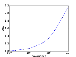
(a) $k=5$, $d=2$.

(b) $k=50$, $d=2$.

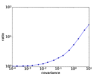
(c) $k=100$, $d=2$.

Figure 4: The ratio of the average $k$-means cost induced by the means over the average optimal cost vs the variance for 2-dimensional instances generated from a mixture of $k$ Gaussians ($k\in\{5,50,100\}$). We observe that the $k$-means objective becomes “relevant” (i.e., is less than 1.05 times the optimal value) for finding the clustering induced by Gaussians when the variance is less than $0.1$ for $k=5$, less than $0.02$ when $k=50$, and less than $0.0005$ when $k=100$.

The results are presented in Figures 4 and 5. We observe that when the variance $\sigma$ is large, the ratio between the average value of the ground truth clustering and the average value of the optimal clustering becomes more important. Indeed, the ground truth clusters start to overlap, allowing to improve the objective value by defining slightly different clusters. Therefore, the use of the $k$-means or $k$-median objectives for modeling the recovery problem is not suitable anymore. In these cases, since Local Search optimizes the solution with respect to the current cost, the clustering output by local search is very different from the ground truth clustering. We thus identify instances for which the $k$-means objective is meaningful and so, Local Search is a relevant heuristic. This motivates the following defintion.

Definition C.3.

We say that a variance $\hat{\sigma}$ is relevant if, for the $k$-means instances generated with variance $\hat{\sigma}$ the ratio between the average value of the ground truth clustering and the optimal clustering is less than 1.05.

We summarize in Table 2 the relevant variances observed.

	$5$	$50$	$100$
2	$<0.05$	$<0.002$	$<0.0005$
10	$<15$	$<1$	$<0.5$
50	$<1000000.0$	$<100$	$<7$

Table 2: Relevant variances for $k\in\{5,50,100\}$ and $d\in\{2,10,50\}$.

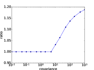
(a) $k=5$, $d=10$.

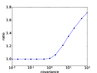
(b) $k=50$, $d=10$.

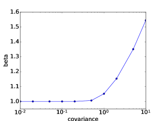
(c) $k=100$, $d=10$.

Figure 5: The ratio of the average $k$-means cost induced by the means over the average optimal cost vs the variance for 10-dimensional instances generated from a mixture of $k$ Gaussians ($k\in\{5,50,100\}$). We observe that the $k$-means objective becomes “relevant” (i.e., is less than 1.05 times the optimal value) for finding the clustering induced by Gaussians when the variance is less than $0.1$ for $k=5$, less than $0.02$ when $k=50$, and less than $0.0005$ when $k=100$.

We consider the $\beta$-distribution-stability condition and ask whether the instances generated from a relevant variance satisfy this condition for constant values of $\beta$. We remark that $\beta$ can take arbitrarily small values.

We thus identify relevant variances (see Table 2) for each pair $k,d$, such that optimizing the $k$-means objective in a $d$-dimensional instances generated from a relevant variance corresponds to finding the underlying clusters.

On stability conditions.

We now study the $\beta$-distribution-stability condition for random instances generated from a mixture of $k$ Gaussians. The results are depicted in Figures 7 and 6.

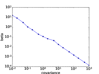
(a) $k=5$, $d=10$.

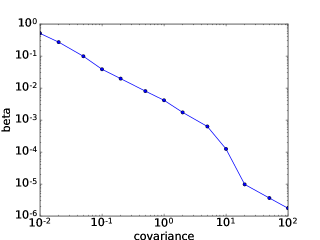
(b) $k=50$, $d=10$.

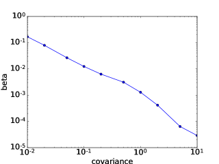
(c) $k=100$, $d=10$.

Figure 6: The average minimum value of $\beta$ for which the instance is $\beta$-distribution-stable vs the variance for 10-dimensional instances generated from a mixture of $k$ Gaussians ($k\in\{5,50,100\}$). We observe that for relevant variances, the value of $\beta$ is greater than $0.001$.

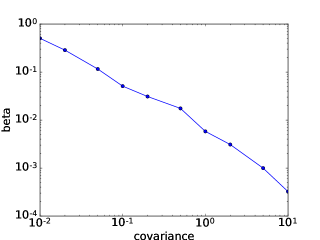
(a) The average minimum value of $\beta$ for which the instances is $\beta$-distribution-stable vs the variance for 2-dimensional instances generated from a mixture of $5$ Gaussians.

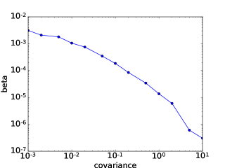
(b) The average of the minimum value of $\beta$ for which the instances is $\beta$-distribution-stable vs the variance for 2-dimensional instances generated from a mixture of $50$ Gaussians.

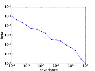
(c) The average minimum value of $\beta$ for which the instance is $\beta$-distribution-stable vs the variance for 2-dimensional instances generated from a mixture of $100$ Gaussians.

Figure 7: The average minimum value of $\beta$ for which the instance is $\beta$-distribution-stable vs the variance for 2-dimensional instances generated from a mixture of $k$ Gaussians ($k\in\{5,50,100\}$). We observe that for relevant variances, the value of $\beta$ is greater than $0.001$.

We observe that for random instances that are not generated from a relevant variance, the instances are $\beta$-distribution-stable for very small values of $\beta$ (e.g., $\beta<1e-07$). We also make the following observation.

Observation C.4.

Instances generated using relevant variances satisfy the $\beta$-distribution-stability condition for $\beta>0.001$.

We remark that the number of dimensions is constant here and that having more dimensions might incur slightly different values for $\beta$. It would be interesting to study this dependency in a new study.

References

- [1] Emile Aarts and Jan K. Lenstra, editors. Local Search in Combinatorial Optimization. John Wiley & Sons, Inc., New York, NY, USA, 1st edition, 1997.
- [2] Dimitris Achlioptas and Frank McSherry. On spectral learning of mixtures of distributions. In Learning Theory, 18th Annual Conference on Learning Theory, COLT 2005, Bertinoro, Italy, June 27-30, 2005, Proceedings, pages 458–469, 2005.
- [3] Sara Ahmadian, Ashkan Norouzi-Fard, Ola Svensson, and Justin Ward. Better guarantees for k-means and euclidean k-median by primal-dual algorithms. CoRR, abs/1612.07925, 2016.
- [4] Ehsan Ardjmand, Namkyu Park, Gary Weckman, and Mohammad Reza Amin-Naseri. The discrete unconscious search and its application to uncapacitated facility location problem. Computers & Industrial Engineering, 73:32 – 40, 2014.
- [5] Ehsan Ardjmand, Namkyu Park, Gary R. Weckman, and Mohammad Reza Amin-Naseri. The discrete unconscious search and its application to uncapacitated facility location problem. Computers & Industrial Engineering, 73:32–40, 2014.
- [6] Sanjeev Arora and Ravi Kannan. Learning mixtures of arbitrary gaussians. In Proceedings on 33rd Annual ACM Symposium on Theory of Computing, July 6-8, 2001, Heraklion, Crete, Greece, pages 247–257, 2001.
- [7] Sanjeev Arora, Prabhakar Raghavan, and Satish Rao. Approximation schemes for Euclidean k-medians and related problems. In Proceedings of the Thirtieth Annual ACM Symposium on the Theory of Computing, Dallas, Texas, USA, May 23-26, 1998, pages 106–113, 1998.
- [8] David Arthur, Bodo Manthey, and Heiko Röglin. Smoothed analysis of the k-means method. J. ACM, 58(5):19, 2011.
- [9] David Arthur and Sergei Vassilvitskii. k-means++: the advantages of careful seeding. In Proceedings of the Eighteenth Annual ACM-SIAM Symposium on Discrete Algorithms, SODA 2007, New Orleans, Louisiana, USA, January 7-9, 2007, pages 1027–1035, 2007.
- [10] David Arthur and Sergei Vassilvitskii. Worst-case and smoothed analysis of the ICP algorithm, with an application to the k-means method. SIAM J. Comput., 39(2):766–782, 2009.
- [11] Vijay Arya, Naveen Garg, Rohit Khandekar, Adam Meyerson, Kamesh Munagala, and Vinayaka Pandit. Local search heuristics for k-median and facility location problems. SIAM J. Comput., 33(3):544–562, 2004.
- [12] Pranjal Awasthi, Avrim Blum, and Or Sheffet. Stability yields a PTAS for k-median and k-means clustering. In 51th Annual IEEE Symposium on Foundations of Computer Science, FOCS 2010, October 23-26, 2010, Las Vegas, Nevada, USA, pages 309–318, 2010.
- [13] Pranjal Awasthi, Avrim Blum, and Or Sheffet. Center-based clustering under perturbation stability. Inf. Process. Lett., 112(1-2):49–54, 2012.
- [14] Pranjal Awasthi, Moses Charikar, Ravishankar Krishnaswamy, and Ali Kemal Sinop. The hardness of approximation of Euclidean k-means. In 31st International Symposium on Computational Geometry, SoCG 2015, June 22-25, 2015, Eindhoven, The Netherlands, pages 754–767, 2015.
- [15] Pranjal Awasthi and Or Sheffet. Improved spectral-norm bounds for clustering. In Approximation, Randomization, and Combinatorial Optimization. Algorithms and Techniques - 15th International Workshop, APPROX 2012, and 16th International Workshop, RANDOM 2012, Cambridge, MA, USA, August 15-17, 2012. Proceedings, pages 37–49, 2012.
- [16] Ainesh Bakshi and Nadiia Chepurko. Polynomial time algorithm for 2-stable clustering instances. CoRR, abs/1607.07431, 2016.
- [17] Maria-Florina Balcan, Avrim Blum, and Anupam Gupta. Approximate clustering without the approximation. In Proceedings of the Twentieth Annual ACM-SIAM Symposium on Discrete Algorithms, SODA 2009, New York, NY, USA, January 4-6, 2009, pages 1068–1077, 2009.
- [18] Maria-Florina Balcan, Avrim Blum, and Anupam Gupta. Clustering under approximation stability. J. ACM, 60(2):8, 2013.
- [19] Maria-Florina Balcan and Mark Braverman. Finding low error clusterings. In COLT 2009 - The 22nd Conference on Learning Theory, Montreal, Quebec, Canada, June 18-21, 2009, 2009.
- [20] Maria-Florina Balcan, Nika Haghtalab, and Colin White. k-center clustering under perturbation resilience. In 43rd International Colloquium on Automata, Languages, and Programming, ICALP 2016, July 11-15, 2016, Rome, Italy, pages 68:1–68:14, 2016.
- [21] Maria-Florina Balcan and Yingyu Liang. Clustering under perturbation resilience. SIAM J. Comput., 45(1):102–155, 2016.
- [22] Maria-Florina Balcan, Heiko Röglin, and Shang-Hua Teng. Agnostic clustering. In Algorithmic Learning Theory, 20th International Conference, ALT 2009, Porto, Portugal, October 3-5, 2009. Proceedings, pages 384–398, 2009.
- [23] Sayan Bandyapadhyay and Kasturi R. Varadarajan. On variants of k-means clustering. CoRR, abs/1512.02985, 2015.
- [24] MohammadHossein Bateni, Aditya Bhaskara, Silvio Lattanzi, and Vahab S. Mirrokni. Distributed balanced clustering via mapping coresets. In Advances in Neural Information Processing Systems 27: Annual Conference on Neural Information Processing Systems 2014, December 8-13 2014, Montreal, Quebec, Canada, pages 2591–2599, 2014.
- [25] Mikhail Belkin and Kaushik Sinha. Polynomial learning of distribution families. In 51th Annual IEEE Symposium on Foundations of Computer Science, FOCS 2010, October 23-26, 2010, Las Vegas, Nevada, USA, pages 103–112, 2010.
- [26] Shai Ben-David, Benny Chor, Oded Goldreich, and Michel Luby. On the theory of average case complexity. Journal of Computer and system Sciences, 44(2):193–219, 1992.
- [27] Shalev Ben-David and Lev Reyzin. Data stability in clustering: A closer look. Theor. Comput. Sci., 558:51–61, 2014.
- [28] Yonatan Bilu, Amit Daniely, Nati Linial, and Michael E. Saks. On the practically interesting instances of MAXCUT. In 30th International Symposium on Theoretical Aspects of Computer Science, STACS 2013, February 27 - March 2, 2013, Kiel, Germany, pages 526–537, 2013.
- [29] Yonatan Bilu and Nathan Linial. Are stable instances easy? Combinatorics, Probability & Computing, 21(5):643–660, 2012.
- [30] Guy E. Blelloch and Kanat Tangwongsan. Parallel approximation algorithms for facility-location problems. In SPAA 2010: Proceedings of the 22nd Annual ACM Symposium on Parallelism in Algorithms and Architectures, Thira, Santorini, Greece, June 13-15, 2010, pages 315–324, 2010.
- [31] Vladimir Braverman, Adam Meyerson, Rafail Ostrovsky, Alan Roytman, Michael Shindler, and Brian Tagiku. Streaming k-means on well-clusterable data. In Proceedings of the Twenty-Second Annual ACM-SIAM Symposium on Discrete Algorithms, SODA 2011, San Francisco, California, USA, January 23-25, 2011, pages 26–40, 2011.
- [32] S. Charles Brubaker and Santosh Vempala. Isotropic PCA and affine-invariant clustering. In 49th Annual IEEE Symposium on Foundations of Computer Science, FOCS 2008, October 25-28, 2008, Philadelphia, PA, USA, pages 551–560, 2008.
- [33] Jaroslaw Byrka, Thomas Pensyl, Bartosz Rybicki, Aravind Srinivasan, and Khoa Trinh. An improved approximation for k-median, and positive correlation in budgeted optimization. In Proceedings of the Twenty-Sixth Annual ACM-SIAM Symposium on Discrete Algorithms, SODA 2015, San Diego, CA, USA, January 4-6, 2015, pages 737–756, 2015.
- [34] Moses Charikar and Sudipto Guha. Improved combinatorial algorithms for facility location problems. SIAM J. Comput., 34(4):803–824, 2005.
- [35] Bernard Chazelle. The discrepancy method - randomness and complexity. Cambridge University Press, 2001.
- [36] Michael B. Cohen, Sam Elder, Cameron Musco, Christopher Musco, and Madalina Persu. Dimensionality reduction for k-means clustering and low rank approximation. In Proceedings of the Forty-Seventh Annual ACM on Symposium on Theory of Computing, STOC 2015, Portland, OR, USA, June 14-17, 2015, pages 163–172, 2015.
- [37] Vincent Cohen-Addad, Philip N. Klein, and Claire Mathieu. Local search yields approximation schemes for k-means and k-median in euclidean and minor-free metrics. In IEEE 57th Annual Symposium on Foundations of Computer Science, FOCS 2016, 9-11 October 2016, Hyatt Regency, New Brunswick, New Jersey, USA, pages 353–364, 2016.
- [38] Vincent Cohen-Addad and Claire Mathieu. Effectiveness of local search for geometric optimization. In 31st International Symposium on Computational Geometry, SoCG 2015, June 22-25, 2015, Eindhoven, The Netherlands, pages 329–343, 2015.
- [39] David Cohen-Steiner, Pierre Alliez, and Mathieu Desbrun. Variational shape approximation. ACM Trans. Graph., 23(3):905–914, 2004.
- [40] Amin Coja-Oghlan. Graph partitioning via adaptive spectral techniques. Combinatorics, Probability & Computing, 19(2):227–284, 2010.
- [41] Anirban Dasgupta, John E. Hopcroft, Ravi Kannan, and Pradipta Prometheus Mitra. Spectral clustering with limited independence. In Proceedings of the Eighteenth Annual ACM-SIAM Symposium on Discrete Algorithms, SODA 2007, New Orleans, Louisiana, USA, January 7-9, 2007, pages 1036–1045, 2007.
- [42] Sanjoy Dasgupta. Learning mixtures of gaussians. In 40th Annual Symposium on Foundations of Computer Science, FOCS ’99, 17-18 October, 1999, New York, NY, USA, pages 634–644, 1999.
- [43] Sanjoy Dasgupta and Yoav Freund. Random projection trees for vector quantization. IEEE Trans. Information Theory, 55(7):3229–3242, 2009.
- [44] Sanjoy Dasgupta and Leonard J. Schulman. A probabilistic analysis of EM for mixtures of separated, spherical gaussians. Journal of Machine Learning Research, 8:203–226, 2007.
- [45] Inderjit S. Dhillon, Yuqiang Guan, and Jacob Kogan. Iterative clustering of high dimensional text data augmented by local search. In Proceedings of the 2002 IEEE International Conference on Data Mining (ICDM 2002), 9-12 December 2002, Maebashi City, Japan, pages 131–138, 2002.
- [46] Daniel B Dias, Renata CB Madeo, Thiago Rocha, Helton H Bíscaro, and Sarajane M Peres. Hand movement recognition for brazilian sign language: a study using distance-based neural networks. In Neural Networks, 2009. IJCNN 2009. International Joint Conference on, pages 697–704. IEEE, 2009.
- [47] Richard O Duda, Peter E Hart, et al. Pattern classification and scene analysis, volume 3. Wiley New York, 1973.
- [48] Dan Feldman and Michael Langberg. A unified framework for approximating and clustering data. In Proceedings of the 43rd ACM Symposium on Theory of Computing, STOC 2011, San Jose, CA, USA, 6-8 June 2011, pages 569–578, 2011.
- [49] Bernd Fischer, Johann Schumann, Wray Buntine, and Alexander G Gray. Automatic derivation of statistical algorithms: The em family and beyond. In Advances in Neural Information Processing Systems, pages 673–680, 2002.
- [50] Ronald A Fisher. The use of multiple measurements in taxonomic problems. Annals of eugenics, 7(2):179–188, 1936.
- [51] Gereon Frahling and Christian Sohler. A fast k-means implementation using coresets. Int. J. Comput. Geometry Appl., 18(6):605–625, 2008.
- [52] Zachary Friggstad, Mohsen Rezapour, and Mohammad R. Salavatipour. Local search yields a PTAS for k-means in doubling metrics. In IEEE 57th Annual Symposium on Foundations of Computer Science, FOCS 2016, 9-11 October 2016, Hyatt Regency, New Brunswick, New Jersey, USA, pages 365–374, 2016.
- [53] Zachary Friggstad and Yifeng Zhang. Tight analysis of a multiple-swap heurstic for budgeted red-blue median. In 43rd International Colloquium on Automata, Languages, and Programming, ICALP 2016, July 11-15, 2016, Rome, Italy, pages 75:1–75:13, 2016.
- [54] Diptesh Ghosh. Neighborhood search heuristics for the uncapacitated facility location problem. European Journal of Operational Research, 150(1):150 – 162, 2003. O.R. Applied to Health Services.
- [55] Diptesh Ghosh. Neighborhood search heuristics for the uncapacitated facility location problem. European Journal of Operational Research, 150(1):150–162, 2003.
- [56] Sudipto Guha and Samir Khuller. Greedy strikes back: Improved facility location algorithms. J. Algorithms, 31(1):228–248, 1999.
- [57] Sudipto Guha, Adam Meyerson, Nina Mishra, Rajeev Motwani, and Liadan O’Callaghan. Clustering data streams: Theory and practice. IEEE Trans. Knowl. Data Eng., 15(3):515–528, 2003.
- [58] Anupam Gupta and Kanat Tangwongsan. Simpler analyses of local search algorithms for facility location. CoRR, abs/0809.2554, 2008.
- [59] Venkatesan Guruswami and Piotr Indyk. Embeddings and non-approximability of geometric problems. In Proceedings of the Fourteenth Annual ACM-SIAM Symposium on Discrete Algorithms, January 12-14, 2003, Baltimore, Maryland, USA., pages 537–538, 2003.
- [60] Pierre Hansen and Nenad Mladenovic. J-m: a new local search heuristic for minimum sum of squares clustering. Pattern Recognition, 34(2):405–413, 2001.
- [61] Pierre Hansen and Nenad Mladenović. Variable neighborhood search: Principles and applications. European journal of operational research, 130(3):449–467, 2001.
- [62] Sariel Har-Peled and Akash Kushal. Smaller coresets for k-median and k-means clustering. Discrete & Computational Geometry, 37(1):3–19, 2007.
- [63] Sariel Har-Peled and Soham Mazumdar. On coresets for k-means and k-median clustering. In Proceedings of the 36th Annual ACM Symposium on Theory of Computing, Chicago, IL, USA, June 13-16, 2004, pages 291–300, 2004.
- [64] Kamal Jain, Mohammad Mahdian, and Amin Saberi. A new greedy approach for facility location problems. In Proceedings on 34th Annual ACM Symposium on Theory of Computing, May 19-21, 2002, Montréal, Québec, Canada, pages 731–740, 2002.
- [65] Kamal Jain and Vijay V. Vazirani. Approximation algorithms for metric facility location and k-median problems using the primal-dual schema and Lagrangian relaxation. J. ACM, 48(2):274–296, 2001.
- [66] Ragesh Jaiswal and Nitin Garg. Analysis of k-means++ for separable data. In Approximation, Randomization, and Combinatorial Optimization. Algorithms and Techniques - 15th International Workshop, APPROX 2012, and 16th International Workshop, RANDOM 2012, Cambridge, MA, USA, August 15-17, 2012. Proceedings, pages 591–602, 2012.
- [67] W. B. Johnson and J. Lindenstrauss. Extensions of Lipschitz mapping into Hilbert space. In Conf. in modern analysis and probability, volume 26 of Contemporary Mathematics, pages 189–206. American Mathematical Society, 1984.
- [68] Ravindran Kannan, Hadi Salmasian, and Santosh Vempala. The spectral method for general mixture models. SIAM J. Comput., 38(3):1141–1156, 2008.
- [69] Tapas Kanungo, David M. Mount, Nathan S. Netanyahu, Christine D. Piatko, Ruth Silverman, and Angela Y. Wu. An efficient k-means clustering algorithm: Analysis and implementation. IEEE Trans. Pattern Anal. Mach. Intell., 24(7):881–892, 2002.
- [70] Tapas Kanungo, David M. Mount, Nathan S. Netanyahu, Christine D. Piatko, Ruth Silverman, and Angela Y. Wu. A local search approximation algorithm for k-means clustering. Comput. Geom., 28(2-3):89–112, 2004.
- [71] Michael Kerber and Sharath Raghvendra. Approximation and streaming algorithms for projective clustering via random projections. In Proceedings of the 27th Canadian Conference on Computational Geometry, CCCG 2015, Kingston, Ontario, Canada, August 10-12, 2015, 2015.
- [72] Stavros G. Kolliopoulos and Satish Rao. A nearly linear-time approximation scheme for the euclidean k-median problem. SIAM J. Comput., 37(3):757–782, June 2007.
- [73] Madhukar R. Korupolu, C. Greg Plaxton, and Rajmohan Rajaraman. Analysis of a local search heuristic for facility location problems. J. Algorithms, 37(1):146–188, 2000.
- [74] Amit Kumar and Ravindran Kannan. Clustering with spectral norm and the k-means algorithm. In 51th Annual IEEE Symposium on Foundations of Computer Science, FOCS 2010, October 23-26, 2010, Las Vegas, Nevada, USA, pages 299–308, 2010.
- [75] Amit Kumar, Yogish Sabharwal, and Sandeep Sen. Linear-time approximation schemes for clustering problems in any dimensions. J. ACM, 57(2), 2010.
- [76] Shrinu Kushagra, Samira Samadi, and Shai Ben-David. Finding meaningful cluster structure amidst background noise. In Algorithmic Learning Theory - 27th International Conference, ALT 2016, Bari, Italy, October 19-21, 2016, Proceedings, pages 339–354, 2016.
- [77] Shi Li and Ola Svensson. Approximating k-median via pseudo-approximation. In Symposium on Theory of Computing Conference, STOC’13, Palo Alto, CA, USA, June 1-4, 2013, pages 901–910, 2013.
- [78] Moshe Lichman. UCI machine learning repository, 2013.
- [79] Meena Mahajan, Prajakta Nimbhorkar, and Kasturi R. Varadarajan. The planar k-means problem is NP-hard. Theor. Comput. Sci., 442:13–21, 2012.
- [80] Konstantin Makarychev and Yury Makarychev. Algorithms for stable and perturbation-resilient problems.
- [81] Jirí Matousek. On approximate geometric k-clustering. Discrete & Computational Geometry, 24(1):61–84, 2000.
- [82] Frank McSherry. Spectral partitioning of random graphs. In 42nd Annual Symposium on Foundations of Computer Science, FOCS 2001, 14-17 October 2001, Las Vegas, Nevada, USA, pages 529–537, 2001.
- [83] Nimrod Megiddo and Kenneth J. Supowit. On the complexity of some common geometric location problems. SIAM J. Comput., 13(1):182–196, 1984.
- [84] Ramgopal R. Mettu and C. Greg Plaxton. The online median problem. SIAM J. Comput., 32(3):816–832, 2003.
- [85] Rafail Ostrovsky, Yuval Rabani, Leonard J. Schulman, and Chaitanya Swamy. The effectiveness of Lloyd-type methods for the k-means problem. J. ACM, 59(6):28, 2012.
- [86] Fabian Pedregosa, Gaël Varoquaux, Alexandre Gramfort, Vincent Michel, Bertrand Thirion, Olivier Grisel, Mathieu Blondel, Peter Prettenhofer, Ron Weiss, Vincent Dubourg, Jake Vanderplas, Alexandre Passos, David Cournapeau, Matthieu Brucher, Matthieu Perrot, and Édouard Duchesnay. Scikit-learn: Machine learning in python. J. Mach. Learn. Res., 12:2825–2830, November 2011.
- [87] Gilles Pisier. The volume of convex bodies and Banach space geometry. Cambridge Tracts in Mathematics. 94, 1999.
- [88] Leonard J. Schulman. Clustering for edge-cost minimization (extended abstract). In Proceedings of the Thirty-Second Annual ACM Symposium on Theory of Computing, May 21-23, 2000, Portland, OR, USA, pages 547–555, 2000.
- [89] Edward Snelson, Carl Edward Rasmussen, and Zoubin Ghahramani. Warped gaussian processes. Advances in neural information processing systems, 16:337–344, 2004.
- [90] Daniel A. Spielman and Shang-Hua Teng. Smoothed analysis of algorithms: Why the simplex algorithm usually takes polynomial time. J. ACM, 51(3):385–463, 2004.
- [91] Minghe Sun. Solving the uncapacitated facility location problem using tabu search. Computers & OR, 33:2563–2589, 2006.
- [92] Dilek Tuzun and Laura I Burke. A two-phase tabu search approach to the location routing problem. European journal of operational research, 116(1):87–99, 1999.
- [93] Dilek Tüzün and Laura I. Burke. A two-phase tabu search approach to the location routing problem. European Journal of Operational Research, 116(1):87–99, 1999.
- [94] Santosh Vempala and Grant Wang. A spectral algorithm for learning mixture models. J. Comput. Syst. Sci., 68(4):841–860, 2004.
- [95] Yi Yang, Min Shao, Sencun Zhu, Bhuvan Urgaonkar, and Guohong Cao. Towards event source unobservability with minimum network traffic in sensor networks. In Proceedings of the First ACM Conference on Wireless Network Security, WISEC 2008, Alexandria, VA, USA, March 31 - April 02, 2008, pages 77–88, 2008.