Kauffman-Jones polynomial of a curve on a surface

Abstract.

We introduce a Kauffman-Jones type polynomial $\mathcal{L}_{\gamma}(A)$ for a curve $\gamma$ on an oriented surface, whose endpoints are on the boundary of the surface. The polynomial $\mathcal{L}_{\gamma}(A)$ is a Laurent polynomial in one variable $A$ and is an invariant of the homotopy class of $\gamma$. As an application, we obtain an estimate in terms of the span of $\mathcal{L}_{\gamma}(A)$ for the minimum self-intersection number of a curve within its homotopy class. We then give a chord diagrammatic description of $\mathcal{L}_{\gamma}(A)$ and show some computational results on the span of $\mathcal{L}_{\gamma}(A)$.

1. Introduction

Let $S$ be an oriented $C^{\infty}$-surface with non-empty boundary $\partial S$. By a curve on $S$, we mean a $C^{\infty}$-immersion $\gamma$ from the unit interval $I=[0,1]$ to $S$, which has only transverse double points as its singularities and satisfies $\gamma^{-1}(\partial S)=\{0,1\}$ with $\gamma(0)\neq\gamma(1)$.

In this article, we consider curves on $S$ from the view point of virtual knots [6] or equivalently, abstract link diagrams [4], with emphasis on their invariants coming from the Kauffman bracket [5]. More concretely, we introduce Laurent polynomials $\langle D_{\gamma}\rangle$ and $\mathcal{L}_{\gamma}(A)$ in one variable $A$. We show that the span of these polynomials can be used for estimating the number of double points of $\gamma$. In fact, the polynomials $\langle D_{\gamma}\rangle$ and $\mathcal{L}_{\gamma}(A)$ depend only on combinatorics of the image of the curve $\gamma$ in its regular neighborhood in $S$. Based on this fact, we then give a chord diagrammatic description of these polynomials. An advantage of being free from the ambient surface $S$ is that it becomes easy to provide and compute examples. In §4, we show some computational results on the span of $\langle D_{\gamma}\rangle$ from this point of view.

In the rest of this section, we describe main constructions and results. Some proofs will be postponed to §2.

We begin with terminology. Let $X$ be a compact 1-manifold. Namely, $X$ is a disjoint union of finitely many $I$’s and circles:

$$X=I\sqcup\dots\sqcup I\sqcup S^{1}\sqcup\dots\sqcup S^{1}.$$

A $C^{\infty}$-immersion $f:X\to S$ is called generic if it has only transeverse double points as its singularities, $f^{-1}(\partial S)=\partial X$, and $f|_{\partial X}$ is injective. A generalized link diagram on $S$ is a subset of $S$ of the form $D=f(X)$ for some generic immersion $f:X\to S$, endowed with a choice of crossing to each double point of $D$. See Figures 2 and 2.

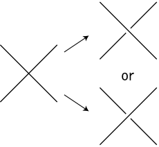
Figure 1. a choice of under- and overcrossing

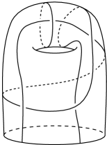
Figure 2. an example of a generalized link diagram

Two generalized link diagrams $D$ and $D^{\prime}$ are called equivalent (resp. regularly equivalent) if $D$ is transformed into $D^{\prime}$ by a finite sequence of ambient isotopies of $S$ relative to $\partial S$, and the three Reidemeister moves $R_{1}$, $R_{2}$, and $R_{3}$ (resp. $R_{2}$ and $R_{3}$) shown in Figure 3. We write $D\sim D^{\prime}$ (resp. $D\sim_{r}D^{\prime}$) when $D$ is equivalent (resp. regularly equivalent) to $D^{\prime}$.

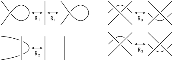
Figure 3. Reidemeister moves

Let $\gamma$ be a curve on $S$. For each double point $p$ of $\gamma$, there is a neighborhood $U$ of $p$ such that $U\cap\gamma(I)$ consists of two arcs $J_{1}$ and $J_{2}$ intersecting at $p$, and $J_{1}$ is traversed first when we go along $\gamma$ from $\gamma(0)$. Then we replace $p$ with a crossing with $J_{1}$ being overcrossing (see Figure 4). Let $D_{\gamma}$ denote the generalized link diagram on $S$ obtained in this way. In other words, $D_{\gamma}$ is the projection diagram in the usual sense of the embedding $I\to S\times I,t\mapsto(\gamma(t),1-t)$ by the projection $S\times I\to S\times\{0\}\cong S,(x,t)\mapsto x$.

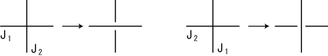
Figure 4. replacing double points with crossings

The following fact is crucial in our argument:

Theorem 1.1.

Suppose that two curves $\gamma$ and $\gamma^{\prime}$ on $S$ are homotopic (resp. regularly homotopic) relative to $\partial S$. Then $D_{\gamma}\sim D_{\gamma^{\prime}}$ (resp. $D_{\gamma}\sim_{r}D_{\gamma^{\prime}}$).

The Kauffman bracket [5] is extended to link diagrams on surfaces [2]. This extension is straightforward and applies to our generalized link diagrams also. For the sake of definiteness, let us recall the construction. Let $D$ be a generalized link diagram on $S$. We can split $D$ at each crossing in two ways. We will distinguish these splittings as a type A splitting and a type B splitting, respectively (see Figures 6 and 6, according to the orientation of $S$). A state of $D$ is a choice of splitting type for each crossing of $D$. For a state $s$ of $D$, let $D(s)$ be the compact 1-submanifold of $S$ obtained by splitting $D$ by $s$. If $D$ has $n$ crossings, there are $2^{n}$ states of $D$.

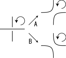
Figure 5. splitting with an orientation

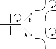
Figure 6. splitting with the other orientation

To each state $s$ of $D$, we assign the following three numbers:

$$\text{$\alpha(s):=$ the number of type A splittings},$$

$$\text{$\beta(s):=$ the number of type B splittings},$$

$$\mu(s):= D(s)$$ the number of connected components of .

Then we define the bracket polynomial of $D$ by

$$\langle D\rangle:=\sum_{s}A^{\alpha(s)-\beta(s)}(-A^{2}-A^{-2})^{\mu(s)-1},$$

where $s$ runs over all states of $D$.

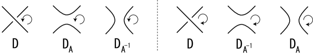
Figure 7. three diagrams

A basic property of the bracket polynomial is the following skein relation, whose proof is the same as that of the classical case [5].

Lemma 1.2.

Let $D$ be a generalized link diagram on $S$.

1. Pick a crossing of $D$ and consider the two splittings of it as shown in Figure 7. Then

   $$\langle D\rangle=A\langle D_{A}\rangle+A^{-1}\langle D_{A^{-1}}\rangle.$$

2. Let $T$ be a generalized link diagram which is connected and has no crossing.

   1. We have $\langle T\rangle=1$.

   2. If $D$ and $T$ are disjoint, then $\langle D\sqcup T\rangle=(-A^{2}-A^{-2})\langle D\rangle$.

Assume that a generalized link diagram $D=f(X)$ is oriented. That is, $X$ is oriented and $D$ inherits this orientation. For instance, if $\gamma$ is a curve on $S$, then $D_{\gamma}$ can be oriented from the natural orientation of $I$. Let $w(D)$ denote the writhe number of $D$. That is,

$$w(D):=\sum_{p}\varepsilon_{p},$$

where $p$ runs over all crossings of $D$ and $\varepsilon_{p}\in\{\pm 1\}$ is the sign of the crossing at $p$ (see Figure 8). Then we define the Kauffman-Jones polynomial of $D$ by

$$\mathcal{L}_{D}(A):=(-A)^{-3w(D)}\langle D\rangle.$$

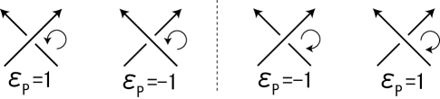
Figure 8. signs of crossings

The following result is an analogy of the result for ordinary link diagrams given by Kauffman [5], where Lemma 1.2 played a central role. His argument can also be applied to the case of generalized link diagrams, so we omit the proof.

Theorem 1.3.

Let $D$ and $D^{\prime}$ be generalized link diagrams on $S$.

1. If $D$ and $D^{\prime}$ are regularly equivalent, $\langle D\rangle=\langle D^{\prime}\rangle$.

2. Assume further that $D$ and $D^{\prime}$ are oriented. If $D$ and $D^{\prime}$ are equivalent, $\mathcal{L}_{D}(A)=\mathcal{L}_{D^{\prime}}(A)$.

To simplify notation, we denote $\mathcal{L}_{\gamma}(A):=\mathcal{L}_{D_{\gamma}}(A)$ for a curve $\gamma$. Combining Theorems 1.1 and 1.3, we obtain

Theorem 1.4.

Let $\gamma$ and $\gamma^{\prime}$ be curves on $S$.

1. If $\gamma$ and $\gamma^{\prime}$ are regularly homotopic relative to $\partial S$, then $\langle D_{\gamma}\rangle=\langle D_{\gamma^{\prime}}\rangle$.

2. If $\gamma$ and $\gamma^{\prime}$ are homotopic relative to $\partial S$, then $\mathcal{L}_{\gamma}(A)=\mathcal{L}_{\gamma^{\prime}}(A)$.

For a Laurent polynomial $f(A)\in\mathbb{Z}[A,A^{-1}]$, the span of $f$, denoted by $\mathrm{span\,}f$, is defined to be the difference of the maximal and the minimal degrees of $f$. Note that $\mathrm{span\,}\langle D_{\gamma}\rangle=\mathrm{span\,}\mathcal{L}_{\gamma}(A)$ for any curve $\gamma$. We denote by $d(\gamma)$ the number of double points of a curve $\gamma$. Then we have the following estimate for $d(\gamma)$, which is analogous to [8] and [9].

Theorem 1.5.

For a curve $\gamma$ on $S$, it holds that

(1.1) $$\mathrm{span\,}\langle D_{\gamma}\rangle\leq 4d(\gamma).$$

We define the minimum self-intersection number $c(\gamma)$ of a curve $\gamma$ by

$$c(\gamma):=\min\,\{\,d(\gamma^{\prime})\,|\,\text{$\gamma^{\prime}$ is a curve on $S$ homotopic to $\gamma$ relative to $\partial S$}\}.$$

Corollary 1.6.

For any curve $\gamma$ on $S$, it holds that

$$\frac{\mathrm{span\,}\langle D_{\gamma}\rangle}{4}\leq c(\gamma).$$

We give examples of using Corollary 1.6 for estimating $c(\gamma)$.

Figure 9. a curve $\gamma_{1}$ on a punctured torus

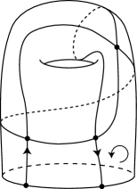
Figure 10. a curve $\gamma_{2}$ on a punctured torus

Example 1.7.

Let $\gamma_{1}$ be the curve shown in Figure 10. The bracket polynomial of $\gamma_{1}$ is

$$\langle D_{\gamma_{1}}\rangle=A-A^{-3}-A^{-5}.$$

We see that $\mathrm{span\,}\langle D_{\gamma_{1}}\rangle=6$ and $6/4\leq c(\gamma_{1})$. Hence we obtain $2\leq c(\gamma_{1})\leq 3$.

Example 1.8.

Let $\gamma_{2}$ be the curve shown in Figure 10. The bracket polynomial of $\gamma_{2}$ is

$$\langle D_{\gamma_{2}}\rangle=-A^{5}+A+A^{-1}-A^{-3}-A^{-5}.$$

Since $\mathrm{span\,}\langle D_{\gamma_{2}}\rangle=10$, we have $10/4\leq c(\gamma_{2})$. Therefore, $c(\gamma_{2})=3$.

2. Proofs of Theorems 1.1 and 1.5

In this section, we prove Theorems 1.1 and 1.5.

Proof of Theorem 1.1.

If two curves $\gamma$ and $\gamma^{\prime}$ are homotopic relative to $\partial S$, then $\gamma$ is transformed into $\gamma^{\prime}$ by using a finite sequence of ambient isotopies of $S$ relative to $\partial S$ and the three local moves $\omega_{1}$, $\omega_{2}$, $\omega_{3}$, shown in Figure 11. See e.g., [1] Lemma 5.6.

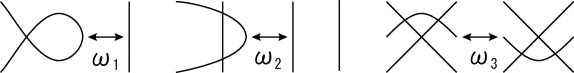
Figure 11. Reidemeister moves of a curve $\gamma$

Figure 12. Reidemeister moves of $\gamma$ and $D_{\gamma}$

It is easily seen that if $\gamma$ is transformed into $\gamma^{\prime}$ by $\omega_{i}$ ($i=1,2,3$), then $D_{\gamma}$ can be transformed into $D_{\gamma^{\prime}}$ by $R_{i}$ ($i=1,2,3$) respectively (see Figure 12). This completes the proof. ∎

Next, we prove Theorem 1.5. Recall that a generalized link diagram $D$ has the form $D=f(X)$ for a generic immersion $f:X\to S$, endowed with a choice of crossing to each double point. We say that $D$ is connected if it is connected as a subset of $S$. Let $d(D)$ be the number of crossings of $D$.

Let us consider the following condition for a generalized link diagram $D=f(X)$:

(2.1) the number of connected components of $$X I$$ homeomorphic to is at most one.

Since $D_{\gamma}$ is connected for any curve $\gamma$, Theorem 1.5 is a special case of the following:

Proposition 2.1.

Let $D$ be a connected generalized link diagram satisfying condition $(\ref{Xform})$. Then it holds that

$$\mathrm{span\,}\langle D\rangle\leq 4d(D).$$

Proof.

The bracket polynomial of $D$ is written as

$$\langle D\rangle=\sum_{s}\langle D|s\rangle\delta^{\mu(s)-1},$$

where $s$ runs over all states of $D$ and we set $\langle D|s\rangle:=A^{\alpha(s)-\beta(s)}$, $\delta:=-A^{2}-A^{-2}$.

Let $s$ be a state of $D$ having a type A splitting, and let $s^{\prime}$ denote the state of $D$ obtained from $s$ by replacing the type A splitting with a type B splitting. Then we have

$$\langle D|s^{\prime}\rangle=\langle D|s\rangle A^{-2},\ \ \mu(s^{\prime})\leq\mu(s)+1,\ \ \mu(s)\leq\mu(s^{\prime})+1.$$

Hence we have

$$\max\ \deg\ \langle D|s^{\prime}\rangle\delta^{\mu(s^{\prime})-1} \leq\max\ \deg\ \langle D|s\rangle\delta^{\mu(s)-1},$$

$$\min\ \deg\ \langle D|s^{\prime}\rangle\delta^{\mu(s^{\prime})-1} \leq\min\ \deg\ \langle D|s\rangle\delta^{\mu(s)-1}.$$

Let $s_{A}$ (resp. $s_{B}$) denote the state of $D$ whose splitting at each crossing is of type A (resp. of type B). Then we have

$$\max\ \deg\ \langle D\rangle \leq\max\ \deg\ \langle D|s_{A}\rangle\delta^{\mu(s_{A})-1}=d(D)+2(\mu(s_{A})-1),$$

$$\min\ \deg\ \langle D\rangle \geq\min\ \deg\ \langle D|s_{B}\rangle\delta^{\mu(s_{B})-1}=-d(D)-2(\mu(s_{B})-1).$$

From these inequalities, we have

$$\mathrm{span\,}\langle D\rangle\leq 2d(D)+2(\mu(s_{A})+\mu(s_{B})-2).$$

Lemma 2.2.

We have $\mu(s_{A})+\mu(s_{B})\leq d(D)+2$.

Proof.

If $d(D)=0$, the inequality is obvious. Let $d(D)>0$ and choose a crossing of $D$ and consider the two splittings of it as shown in Figure 7. Then, at least one of them is connected and satisfies condition (2.1) by virtue of the assumption (2.1) on $D$. Let $D^{\prime}$ be such a generalized link diagram and assume that $D^{\prime}$ is obtained from the type A splitting (the other case is treated similarly). Let $s_{A}^{\prime}$ and $s_{B}^{\prime}$ be the states of $D^{\prime}$ defined by the same way as we introduce $s_{A}$ and $s_{B}$ to $D$. Then $\mu(s_{A})=\mu(s_{A}^{\prime})$ and $\mu(s_{B})\leq\mu(s_{B}^{\prime})+1$, hence $\mu(s_{A})+\mu(s_{B})\leq\mu(s^{\prime}_{A})+\mu(s^{\prime}_{B})+1$. Then the assertion is proved by induction on $d(D)$. ∎

By Lemma 2.2 we conclude

$$\mathrm{span\,}\langle D\rangle\leq 2d(D)+2(\mu(s_{A})+\mu(s_{B})-2)\leq 4d(D).$$

This completes the proof of Proposition 2.1. ∎

3. Chord diagrammatic description

For a curve $\gamma$ on $S$, the bracket polynomial $\langle D_{\gamma}\rangle$ is actually determined by a regular neighborhood of $\gamma(I)$ in $S$. In this section, we study $\langle D_{\gamma}\rangle$ from this point of view.

Let $d$ be a positive integer. An oriented linear chord diagram of $d$ chords is a set $C=\{(i_{1},j_{1}),\ldots,(i_{d},j_{d})\}$ of $d$ ordered pairs of integers such that $\{i_{k}\}_{k}\cup\{j_{k}\}_{k}=\{1,\ldots,2d\}$. Each element of $C$ is called a chord of $C$. A chord $(i,j)$ is called positive if $i<j$, and negative otherwise. Finally, a state of $C$ is a map $s\colon C\to\{A,B\}$, where $A$ and $B$ are fixed symbols.

Let $\gamma$ be a curve with $d(\gamma)=d$. Then the inverse image of the double points of $\gamma$ are $2d$ points on $I$. We name them $\{p_{i}\}_{i}$ so that $0<p_{1}<p_{2}<\cdots<p_{2d}<1$. The oriented linear chord diagram $C_{\gamma}$ is defined by the condition that an ordered pair $(i,j)$ is a chord of $C_{\gamma}$ if and only if $\gamma(p_{i})=\gamma(p_{j})$ and the pair $(d\gamma/dt(p_{i}),d\gamma/dt(p_{j}))$ of tangent vectors matches the orientation of $S$.

Remark 3.1.

Conversely, for any oriented linear chord diagram $C$, there is a curve $\gamma$ on some oriented surface $S$ such that $C=C_{\gamma}$.

Let $C$ be an oriented linear chord diagram of $d$ chords and $s$ a state of $C$. For each chord $c=(i,j)\in C$, we define a subset $R_{c}\subset\mathfrak{S}_{2d+1}$ of permutations of $2d+1$ letters $\{0,1,\ldots,2d\}$ in the following way.

• If $s(c)=A$ and $c$ is positive, or $s(c)=B$ and $c$ is negative, then we set $R_{c}=\{(i,j-1),(i-1,j)\}$.

• If $s(c)=A$ and $c$ is negative, or $s(c)=B$ and $c$ is positive, then we set $R_{c}=\{(i,j),(i-1,j-1)\}$.

Consider the subgroup of $\mathfrak{S}_{2d+1}$ generated by $\bigcup_{c\in C}R_{c}$, and let $\Gamma_{s}$ be the number of orbits of the action of this group on $\{0,\ldots,2d\}$.

We set

$$\langle C|s\rangle:=A^{|s^{-1}(A)|-|s^{-1}(B)|}(-A^{2}-A^{-2})^{\Gamma_{s}-1},$$

where $|s^{-1}(A)|$ denotes the cardinality of the set $s^{-1}(A)$, and we define

$$\langle C\rangle:=\sum_{s}\langle C|s\rangle,$$

where the sum runs over all states of $C$. We also define

$$\mathcal{L}_{C}(A):=(-A)^{-3w(C)}\langle C\rangle,$$

where $w(C)$ is the number of positive chords minus the number of negative chords of $C$.

Proposition 3.2.

Let $\gamma$ be a curve on $S$. Then $\langle D_{\gamma}\rangle=\langle C_{\gamma}\rangle$ and $\mathcal{L}_{\gamma}(A)=\mathcal{L}_{C_{\gamma}}(A)$.

Proof.

First of all, the second formula follows from the first, since $w(D_{\gamma})=w(C_{\gamma})$.

Now introduce $2d+1$ points $q_{i}$, $0\leq i\leq 2d$. With respect to the parametrization of $\gamma$, these points have the following interpretation: $q_{0}=0$, $q_{i}=(p_{i}+p_{i+1})/2$ for $1\leq i\leq 2d-1$, and $q_{2d}=1$. For a state $s$ of $\gamma$, let $\Gamma(C_{\gamma},s)$ be the graph with the set of vertices being $\{q_{i}\}_{i}$, and the set of edges determined by the condition that $q_{k}$ and $q_{l}$ are connected by an edge if and only if $(k,l)\in\bigcup_{c\in C_{\gamma}}R_{c}$. Then $\Gamma(C_{\gamma},s)$ is homeomorphic to the splice of $D_{\gamma}$ by $s$. See Figure 13. (Here and in what follows, we assume the counter-clockwise orientation in any figure.) The first formula follows from this observation. ∎

Figure 13. proof of Proposition 3.2

In the below, we record elementary properties of $\langle D_{\gamma}\rangle$ in terms of chord diagrams.

Let $C=\{(i_{1},j_{1}),\ldots,(i_{d},j_{d})\}$ be an oriented linear chord diagram. Fix $0\leq\ell\leq 2d$. For $i\in\{1,\ldots,2d\}$, we set

$$i^{\prime}:=\begin{cases}i&\quad\text{if $i\leq\ell$},\\ i+2&\quad\text{if $i>\ell$}.\end{cases}$$

We define

$$C_{+}^{\ell} :=\{(i^{\prime}_{k},j^{\prime}_{k})\}_{k}\cup\{(\ell,\ell+1)\},$$

$$C_{-}^{\ell} :=\{(i^{\prime}_{k},j^{\prime}_{k})\}_{k}\cup\{(\ell+1,\ell)\}.$$

Also, we define

$$C_{+}^{\wedge} :=\{(i_{k}+1,j_{k}+1)\}_{k}\cup\{(1,2d+2)\},$$

$$C_{-}^{\wedge} :=\{(i_{k}+1,j_{k}+1)\}_{k}\cup\{(2d+2,1)\}.$$

Proposition 3.3 (Birth/death of monogons).

We have

$$\langle C_{+}^{\ell}\rangle=\langle C_{+}^{\wedge}\rangle=(-A^{3})\langle C\rangle,$$

$$\langle C_{-}^{\ell}\rangle=\langle C_{-}^{\wedge}\rangle=(-A^{-3})\langle C\rangle.$$

Proof.

If $C=C_{\gamma}$ for some curve $\gamma$, then $C_{+}^{\ell}$ corresponds to a suitable insertion of a negative monogon to $\gamma$. Therefore, from the behavior of the bracket polynomial under the Reidemeister move $R_{1}$, we obtain $\langle C_{+}^{\ell}\rangle=(-A^{3})\langle C\rangle$. The other cases are treated similarly. ∎

Let

$$C=\{(i_{1},j_{1}),\ldots,(i_{d},j_{d})\}\quad\text{and}\quad D=\{(k_{1},\ell_{1}),\ldots,(k_{e},\ell_{e})\}$$

be oriented linear chord diagrams. We define the stacking of $C$ and $D$ by

$$C\sharp D:=\{(i_{a},j_{a})\}_{a}\cup\{(k_{b}+2d,\ell_{b}+2d)\}_{b}.$$

Proposition 3.4 (Stacking formula).

We have $\langle C\sharp D\rangle=\langle C\rangle\langle D\rangle$. In particular, $\mathrm{span\,}\langle C\sharp D\rangle=\mathrm{span\,}\langle C\rangle+\mathrm{span\,}\langle D\rangle$.

Proof.

Since the chords of $C\sharp D$ are in one-to-one correspondence with the disjoint union of the chords of $C$ and $D$, any state of $C\sharp D$ is of the form $s\sharp t$, where $s$ is a state of $C$ and $t$ is a state of $D$. The assertion follows from the observation that $|\Gamma(C\sharp D,s\sharp t)|=|\Gamma(C,s)|+|\Gamma(D,t)|-1$. ∎

Proposition 3.5.

Let $C$ be an oriented linear chord diagram of $d$ chords.

• If $d$ is even, then $\langle C\rangle$ has only terms of even degree.

• If $d$ is odd, then $\langle C\rangle$ has only terms of odd degree.

Proof.

By definition, $\langle C|s\rangle$ has this property, so does $\langle C\rangle$. ∎

Proposition 3.6 (Reversing all the chords).

Let $C=\{(i_{1},j_{1}),\ldots,(i_{d},j_{d})\}$ be an oriented linear chord diagram and set $\overline{C}:=\{(j_{1},i_{1}),\ldots,(j_{d},i_{d})\}$. Then $\langle\overline{C}\rangle=\langle C\rangle|_{A\mapsto A^{-1}}$.

Proof.

There is a natural bijection $\iota$ from the set of chords of $C$ to that of $\overline{C}$ given by $(i_{k},j_{k})\mapsto(j_{k},i_{k})$. This maps positive (resp. negative) chords to negative (resp. positive) chords. Moreover, it induces a bijection from the set of states of $C$ to that of $\overline{C}$ given by $s\mapsto\overline{s}$, determined by the condition that $\{s(c),\overline{s}(\iota(c))\}=\{A,B\}$ for any chord $c$ of $C$. Then, it holds that $\langle C|s\rangle=\langle\overline{C}|\overline{s}\rangle|_{A\mapsto A^{-1}}$ for any state $s$ of $C$. This proves the formula. ∎

4. The range of the span

In this section, we study the range of $\mathrm{span\,}\langle C\rangle$. By Theorem 1.5, $\mathrm{span\,}\langle C\rangle\leq 4d$ if $C$ has $d$ chords. Also, by Proposition 3.5, $\mathrm{span\,}\langle C\rangle$ is always an even integer. Fixing $d$, let us consider which even integers not greater than $4d$ are realized as $\mathrm{span\,}\langle C\rangle$ for some $C$ with $d$ chords.

We say that an even integer $l$ is $d$-realizable if there exists an oriented linear chord diagram $C$ of $d$ chords such that $\mathrm{span\,}\langle C\rangle=l$.

If $d=1$, $C=C_{1}:=\{(1,2)\}$ or $C=\overline{C_{1}}$. Thus $\langle C\rangle=-A^{\pm 3}$ and $\mathrm{span\,}\langle C\rangle=0$.

If $d=2$, by a direct computation, we see that $0$ and $6$ are $2$-realizable, while $2$, $4$, and $8$ are not. For example, $C_{2}=\{(1,3),(2,4)\}$ satisfies $\langle C_{2}\rangle=A^{2}+1-A^{-4}$, so that $\mathrm{span\,}\langle C_{2}\rangle=6$.

If $d=3$, we see that $0$, $6$, $10$, and $12$ are $3$-realizable, while $2$, $4$, and $8$ are not. For example, the stacking $C_{1}\sharp C_{2}$ satisfies $\mathrm{span\,}\langle C_{1}\sharp C_{2}\rangle=6$; $C_{3}=\{(1,5),(2,4),(6,3)\}$ satisfies $\langle C_{3}\rangle=-A^{5}-A^{3}+A+A^{-1}-A^{-5}$, so that $\mathrm{span\,}\langle C_{3}\rangle=10$; the chord diagram $C(3)$ in Example 4.1 below satisfies $\mathrm{span\,}\langle C(3)\rangle=12$.

To see the case $d\geq 4$, we consider the following two examples.

Example 4.1.

Let $d\geq 1$ be an odd integer, and set $C(d):=\{(i,i+d)\}_{i=1}^{d}.$ Then

$$\langle C(d)\rangle=\sum_{i=1}^{d-1}(-1)^{i-1}A^{-3d-2+4i}-A^{d+2}.$$

In particular, if $d\geq 3$, then $\mathrm{span\,}\langle C\rangle=(d+2)-(-3d+2)=4d$.

Figure 14. the curve $\gamma_{d}$ in Example 4.1

Proof.

We have $C(d)=C_{\gamma_{d}}$, where $\gamma_{d}$ is the curve as shown in Figure 14. Let $d\geq 1$ be an odd integer. Then

$$\hskip 40.00006pt=A^{2}\langle\gamma_{d}\rangle+(-A^{-3})^{d}+A^{-3d-4}.$$

Now it is easy to see that $\langle\gamma_{1}\rangle=-A^{3}$, and the formula is proved by an inductive argument. ∎

Example 4.2.

Let $d\geq 4$ be an even integer, and set

$$C(d):=\{(1,d),(d+1,2d)\}\cup\{(2d-i,i+1)\}_{i=1}^{d-2}.$$

Then

$$\langle C(d)\rangle=A^{-3d+4}-A^{-3d+8}+2\left(\sum_{i=1}^{d-4}(-1)^{i-1}A^{-3d+8+4i}\right)+A^{d-4}-A^{d}+A^{d+4}.$$

In particular, $\mathrm{span\,}\langle C(d)\rangle=(d+4)-(-3d+4)=4d$.

Figure 15. the curve $\gamma_{d}$ in Example 4.2

Proof.

We have $C(d)=C_{\gamma_{d}}$, where $\gamma_{d}$ is the curve as shown in Figure 15. Let $d\geq 4$ be an even integer. Then

The diagram in the first term of (4) can be expanded as

On the other hand, the second term of (4) is equal to

Moreover, we compute

$$= A(-A^{3})+A^{-1}(-A^{-3})=-A^{-4}-A^{4}.$$

Therefore, we obtain

$$\langle\gamma_{d+2}\rangle= A^{2}\langle\gamma_{d}\rangle+((-A^{-3})^{d-2}+A^{-1}\cdot(-A^{-3})^{d-1})(-A^{-4}-A^{4})$$

$$= A^{2}\langle\gamma_{d}\rangle+A^{-3d-2}-A^{-3d+2}+A^{-3d+6}-A^{-3d+10}.$$

Now, by a direct computation, we see that $\langle\gamma_{4}\rangle=A^{-8}-A^{-4}+1-A^{4}+A^{8}$, and the formula is proved by an inductive argument. ∎

Theorem 4.3.

Let $d\geq 4$. Any even integer $l\in\{0,6,8,\ldots,4d\}$ is $d$-realizable.

Proof.

Let $d=4$. First, $0$, $6$, $10$, and $12$ are $4$-realizable. To see this, for any $l\in\{0,6,10,12\}$ pick an oriented chord diagram $D$ of $3$ chords with $\mathrm{span\,}D=l$; then the stacking $C=C_{1}\sharp D$ satisfies $\mathrm{span\,}\langle C\rangle=l$. Next, $8$ is $4$-realizable, since $C_{4}=\{(1,4),(2,7),(3,5),(6,8)\}$ satisfies $\langle C_{4}\rangle=A^{4}+A^{2}+1-A^{-2}-A^{-4}$, so that $\mathrm{span\,}\langle C_{4}\rangle=8$; also $14$ is $4$-realizable, since $C^{\prime}_{4}=\{(1,5),(2,4),(3,7),(6,8)\}$ satisfies $\langle C^{\prime}_{4}\rangle=A^{8}+A^{6}-A^{4}-A^{2}+1+A^{-2}-A^{-6}$, so that $\mathrm{span\,}\langle C^{\prime}_{4}\rangle=14$. Finally, the element $C(4)$ in Example 4.2 satisfies $\mathrm{span\,}\langle C(4)\rangle=16$.

Now let $d\geq 5$ and assume that any even integer $l\in\{0,6,8,\ldots,4(d-1)\}$ is $(d-1)$-realizable. Then by considering the stacking of $C_{1}$ and oriented linear chord diagrams of $d-1$ chords, we see that any $l\in\{0,6,8,\ldots,4(d-1)\}$ is $d$-realizable. Next, the element $C(d)$ in Examples 4.1 and 4.2 satisfies $\mathrm{span\,}\langle C(d)\rangle=4d$. Finally, the stacking $C=C_{2}\sharp C(d-2)$ satisfies $\mathrm{span\,}\langle C\rangle=6+4(d-2)=4d-2$.

By induction on $d$, we obtain the assertion. ∎

It can be checked that $2$ and $4$ are not $d$-realizable for $d\leq 6$.

Question 4.4.

Is there an oriented linear chord diagram $C$ such that $\mathrm{span\,}\langle C\rangle=2$ or $4$?

Finally, we study the case where the equality $\mathrm{span\,}\langle C\rangle=4d$ holds. This class of linear chord diagrams might be of interest since it is closed under stacking by Proposition 3.4. Table 1 shows the number of linear chord diagrams with $\mathrm{span\,}\langle C\rangle=4d$ for a fixed integer $d\leq 9$. To give another motivation, let us recall the following classical result on characterization of alternating knots.

Table 1. linear chord diagrams with $\mathrm{span\,}\langle C\rangle=4d$

$d$	2	3	4	5	6	7	8	9
	0	2	4	12	84	338	1588	8588

Theorem 4.5 ([5] [8] [9]).

Let $K$ be an oriented knot in $S^{3}$ and assume that the span of the Jones polynomial $V_{K}(t)=\mathcal{L}_{K}(t^{-1/4})$ is equal to the minimum number of double points among all projection diagrams of $K$. Then $K$ is alternating.

Let $C$ be an oriented linear chord diagram of $d$ chords, and let $\gamma$ be a curve on an oriented surface $S$ such that $C_{\gamma}=C$. Let $s_{A}$ and $s_{B}$ be the states of $D_{\gamma}$ which appeared in the proof of Proposition 2.1. Suppose that $\mathrm{span\,}\langle C\rangle=4d$. Then, as we see from the proof of Proposition 2.1, we have

(4.2) $$\mu(s_{A})+\mu(s_{B})=d+2.$$

Remark 4.6.

The condition (4.2) does not imply $\mathrm{span\,}\langle C\rangle=4d$. For example, let $C=\{(1,8),(2,5),(3,6),(4,7)\}$. Then $\mu(s_{A})+\mu(s_{B})=6$. However, $\langle C\rangle=A^{8}+1-A^{-4}$ and $\mathrm{span\,}\langle C\rangle=12\neq 16$.

Let us consider the following condition for $C$.

(4.3) for any chord $$(i,j) C i j$$ of , the parity of and are different.

Theorem 4.7.

Keep the notation as above. Then condition $(\ref{eq:sasb})$ implies condition $(\ref{eq:parity})$. In particular, if $\mathrm{span\,}\langle C\rangle=4d$, then condition $(\ref{eq:parity})$ holds.

To prove this, let us consider the following preliminary construction. Let $N$ be a regular neighborhood of $\gamma$ in $S$. We modify $N$ in a neighborhood of every double point of $\gamma$ by inserting two half-twisted bands as illustrated in Figure 16. The result is denoted by $N^{\prime}$, in which the curve $\gamma$ embeds naturally. Next, we give a labelling $A$ or $B$ to each boundary component of a neighborhood in $N^{\prime}$ of each double point as shown in Figure 16. Then, this labelling extends naturally to a locally constant function $\phi\colon\partial N^{\prime}\setminus\partial S\to\{A,B\}$. From the construction, we see that the inverse image $\phi^{-1}(A)$ (resp. $\phi^{-1}(B)$) is homeomorphic to the splice of $D_{\gamma}$ by $s_{A}$ (resp. $s_{B}$). Therefore, if we denote by $r^{\prime}$ the number of boundary components of $N^{\prime}$, we have

(4.4) $$r^{\prime}=\mu(s_{A})+\mu(s_{B})-1.$$

Figure 16. the construction of the surface $N^{\prime}$

Lemma 4.8.

The surface $N^{\prime}$ is orientable if and only if condition $(\ref{eq:parity})$ holds.

Proof.

Let $\{p_{k}\}_{k=1}^{d}$ be the set of double points of $\gamma$, and fix a parametrization $\gamma\colon I\to S$. For each $k$, write $\gamma^{-1}(p_{k})=\{t^{1}_{k},t^{2}_{k}\}$ so that $t^{1}_{k}<t^{2}_{k}$, and let $c_{k}\in H_{1}(N^{\prime};\mathbb{Z})$ be the homology class of the loop defined as the restriction of $\gamma$ to $[t^{1}_{k},t^{2}_{k}]$. Then, the set $\{c_{k}\}_{k=1}^{d}$ constitutes a $\mathbb{Z}$-basis for $H_{1}(N^{\prime};\mathbb{Z})$.

Now, let $w_{1}\in H^{1}(N^{\prime};\mathbb{Z}_{2})\cong{\rm Hom}(H_{1}(N^{\prime};\mathbb{Z}),\mathbb{Z}_{2})$ be the first Stiefel-Whitney class of the tangent bundle of $N^{\prime}$. Let $(i_{k},j_{k})$ be the chord of $C$ corresponding to $p_{k}$. Then, $w_{1}(c_{k})$ is just the number of inserted half-twisted bands along the representative of $c_{k}$, and this is equal to $|i_{k}-j_{k}|+1$. Since $N^{\prime}$ is orientable if and only if $w_{1}=0$, the assertion follows. ∎

Proof of Theorem 4.7.

Since $N^{\prime}$ is homotopy equivalent to the bouquet of $d$ circles, the Euler characteristic of $N^{\prime}$ is $\chi(N^{\prime})=1-d$.

Assume that $N^{\prime}$ is unorientable. Since $r^{\prime}=d+1$ from (4.2) and (4.4), there exists an integer $g>0$ and $N^{\prime}$ is homeomorphic to a connected sum of $g$ copies of $\mathbb{R}P^{2}$ minus the interior of $d+1$ disjoint union of closed disks. Hence

$$\chi(N^{\prime})=2-g-(d+1)=1-g-d.$$

Thus $g=0$, a contradiction. Therefore $N^{\prime}$ is orientable, and the conclusion follows by Lemma 4.8. ∎

Acknowledgements. The authors would like to thank Haruko Miyazawa and Akira Yasuhara for their helpful comments. S. F. was supported by JSPS KAKENHI 26400098. Y. K. was supported by JSPS KAKENHI 26800044.

References

[1]
Goldman, W. M.:
Invariant functions on Lie groups and Hamiltonian flows of surface group representations,
Invent. Math.
85 (1986),
263–302.
[2]
Inoue, K. and Kaneto, T.:
A Jones type invariant of links in the product space of a surface and the real line,
J. Knot Theory Ramifications
94 (1994),
153–161.
[3]
Jones, V. F. R.:
A polynomial invariant for knots via Von Neumann algebras,
Bull. Amer. Math. Soc. 12 (1985),
103–111.
[4]
Kamada, N. and Kamada, S.:
Abstract link diagrams and virtual knots,
J. Knot Theory Ramifications
9 (2000),
93–106.
[5]
Kauffman, L. H.:
State models and the Jones polynomial,
Topology
26 (1987),
395–407.
[6]
Kauffman, L. H.:
Virtual knot theory,
Europ. J. Combinatorics
20 (1999),
663–691.
[7]
Manturov, V. O.:
Kauffman-like polynomial and curves in -surfaces,
J. Knot Theory Ramifications
12 (2003),
1145–1153.
[8]
Murasugi, K.:
Jones polynomials and classical conjectures in knot theory,
Topology
26 (1987),
187–194.
[9]
Thistlethwaite, M. B.:
A spanning tree expansion of the Jones polynomial,
Topology
26 (1987),
297–309.