Abstract

Some equivalence classes in symmetric group lead to an interesting class of noncommutive and associative algebras. From these algebras we construct noncommutative Frobenius algebras. Based on the correspondence between Frobenius algebras and two-dimensional topological field theories, the noncommutative Frobenius algebras can be interpreted as topological open string theories. It is observed that the centre of the algebras are related to closed string theories via open-closed duality. Area-dependent two-dimensional field theories are also studied.

1 Introduction

Topological field theories are the simplest field theories whose amplitudes are indepedendent of the local Riemann structure. Two-dimensional topological field theories may attract a particular interest because they can be regarded as toy models of string theory. If we ignore the conformal structure of Riemann surfaces corresponding to worldsheets, we have two-dimensional topological field theories [1, 2].

In this paper we will focus on the one-to-one correspondence between two-dimensional topological field theories and Frobenius algebras [3, 4, 5, 6]. This may suggest an interesting story that two-dimensional topological field theories can be re-constructed from a certain kind of algebras, which reminds us of some recent approaches of string theory that it is re-constructed from discrete data like matrices in AdS/CFT correspondence and the matrix models.

A Frobenius algebra is defined as a finite-dimensional associative algebra equipped with a non-degenerate bilinear form. Given an associative algebra, it can be a Frobenius algebra by specifying the bilinear form. It is emphasised that being Frobenius is not a property of the algebra, but it is a structure we provide. We can construct different Frobenius algebras by giving different Frobenius structures, even though the underlying algebra is the same. For a Frobenius algebra, we can associate the bilinear form and the structure constant with the propagator and the three-point vertex of a two-dimensional topological field theory. Topological properties of the theory can be explained from the fact that it is an associative algebra with a non-degenerate bilinear form.

Our interest on the equivalence comes from the recent development that correlation functions of the Gaussian matrix models, encoding the space-time independent part of correlation functions of ${\cal N}=4$ Super Yang-Mills, are expressed in terms of elements in associative algebras obtained from symmetric group.

In section 2 we introduce some associative algebras obtained from the group algebra of the symmetric group. Sums of all elements in the conjugacy classes are central elements in the group algebra, and the product is closed. They form an associative and commutative algebra. We can also construct more general class of algebras by introducing equivalence relations in terms of elements in subgroups of the symmetric group [9, 10, 11]. Such algebras are associative but in general noncommutative. Because the noncommutativity is related to the restriction from the symmetric group to the subalgebra, the noncommutative structure is sometimes referred to as restricted structure. Some algebras with restricted structure were recently studied in [12].

In section 3, we will explain how the algebras introduced in section 2 appear in the description of gauge invariant operators in ${\cal N}=4$ Super Yang-Mills. The elements in the algebras have an one-to-one correspondence with the gauge invariant operators. Two-point functions of the gauge invariant operators give a map from two elements in the algebra to a $c$-number. Regarding the map as a bilinear form, we can introduce Frobenius algebras naturally from the matrix models. The equivalence between Frobenius algebras and two-dimensional topological field theories leads to an interpretation of correlation functions of the matrix models in terms of two-dimensional topological field theories [13].

In section 4, we will review concretely how Frobenius algebras describe topological field theories. Commutative Frobenius algebras correspond to topological closed string theories, while noncommutative Frobenius algebras can be associated with open string theories [3, 4, 7, 8]. Because the closed propagator is related to a non-planar one-loop diagram of an open string theory, the closed string theory and the open string theory should be described in a unified algebraic framework. Our review will be given from this point of view.

Section 5 will be devoted to a detailed study of algebras with the restricted structure from the point of view of the open-closed duality. In our previous paper [14] correlation functions of topological field theories related to noncommutative Frobenius algebras were studied. In this paper, we reinterpret the noncommutative Frobenius algebras as open string theories. Elements in the noncommutative algebras are related to open string states, while the centre of the algebra describes closed string states. The restricted structure may cause an area-dependence in correlation functions of the closed string theories.

In section 6 we summarise this paper. In appendices, we give formulas, detailed computations and additional explanations. Appendices of our previous paper [14] may also be helpful to check equations of this paper.

This paper is based on the talk “ Noncommutative Frobenius algebras and open strigns,” given in workshop “ Permutations and Gauge String duality,” held at Queen Mary, University of London at July 2014. The relationship to our recent work [15] is also briefly mentioned.

2 Equivalence classes in symmetric group

We consider some types of equivalence classes in symmetric group $S_{n}$. One is the conjugacy classes. The others are introduced by considering subgroups, which leads to an interesting class of algebras.

Consider the group algebra of $S_{n}$ over $\mathbb{C}$, which is called $\mathbb{C}[S_{n}]$. For elements in $S_{n}$, introduce the equivalence relation $\sigma\sim g\sigma g^{-1}$ by any element $g$ in $S_{n}$. Because of the equivalence relation, the set of elements in $S_{n}$ are classified into conjugacy classes. It is then convenient to consider

$$[\sigma]=\frac{1}{n!}\sum_{\tau\in S_{n}}\tau\sigma\tau^{-1}.$$ (1)

Elements in a conjugacy class give the same value of $[\sigma]$, i.e. we have

$$[\sigma]=[g\sigma g^{-1}]$$ (2)

for any $g$ in $S_{n}$. In fact $[\sigma]$ is the sum of all elements in the conjugacy class the $\sigma$ belongs to. The sums are central elements in $\mathbb{C}[S_{n}]$,

$$[\sigma]\tau=\tau[\sigma],\quad[\sigma][\tau]=[\tau][\sigma]$$ (3)

for any $\sigma,\tau\in S_{n}$. Because $\sigma$ and $\sigma^{-1}$ are in the same conjugacy class, we also have

$$[\sigma]=[\sigma^{-1}].$$ (4)

The product of two central elements gives a central element of the form (1),

$$[\sigma_{1}][\sigma_{2}]=\frac{1}{n!}\sum_{\tau\in S_{n}}\tau\sigma_{1}[\sigma_{2}]\tau^{-1}.$$ (5)

As above the $[\sigma]$ span a basis of the centre of the group algebra. Central elements form a closed commutative and associative algebra, which is denoted by $Z(\mathbb{C}[S_{n}])$.

We next introduce the equivalence relation determined by a subgroup $H$ of $S_{n}$ as $\sigma\sim h\sigma h^{-1}$, where $h\in H$ and $\sigma\in S_{n}$. Generalising (1), the equivalence classes under the subgroup $H$ are classified by

$$[\sigma]_{H}=\frac{1}{|H|}\sum_{h\in H}h\sigma h^{-1},$$ (6)

where $|H|$ denotes the dimension of the subgroup. They have the following properties

$$[\sigma]_{H}=[h\sigma h^{-1}]_{H},\quad h[\sigma]_{H}=[\sigma]_{H}h\quad(h\in H),$$ (7)

and also

$$[\sigma]_{H}\neq[\sigma^{-1}]_{H}.$$ (8)

The product of two elements of the form (6) can be expressed by the form (6),

$$[\sigma_{1}]_{H}[\sigma_{2}]_{H}=\frac{1}{|H|}\sum_{h\in H}h\sigma_{1}[\sigma_{2}]_{H}h^{-1}.$$ (9)

The closed algebra formed by the elements (6) is called $\mathbb{C}[S_{n}]_{H}$ in this paper. Our notation is that $\mathbb{C}[S_{n}]_{H}=Z(\mathbb{C}[S_{n}])$ for $H=S_{n}$. A big difference from the algebra relevant for the conjugacy classes is that the elements given in (6) span a noncommutative algebra,

$$[\sigma]_{H}[\tau]_{H}\neq[\tau]_{H}[\sigma]_{H}.$$ (10)

There are several interesting subgroups we can choose for $H$. For instance we choose $H=S_{n_{1}}\times S_{n_{2}}\times\cdots$, where $n_{1}+n_{2}=\cdots=n$ [9, 11, 19]. It is also interesting to consider the wreath product group $H=S_{n/2}[S_{2}]$, which has played a role recently in [15].

Brauer algebras can also be similarly considered. The walled Brauer algebra $B(n_{1},n_{2})$ with the subgroup $H=S_{n_{1}}\times S_{n_{2}}$ gives equivalence classes determined by

$$[b]_{H}=\frac{1}{n_{1}!n_{2}!}\sum_{h\in S_{n_{1}}\times S_{n_{2}}}hbh^{-1},$$ (11)

where $b$ is an element in the walled Brauer algebra. These quantities can classify a certain class of gauge invariant operators [10, 16].

Before closing this section, we shall give a remark about another basis labelled by a set of representation labels. We may use the projection operators as a basis of $Z(\mathbb{C}[S_{n}])$. The change of basis is given by

$$[\sigma]=\sum_{R\vdash n}\frac{1}{d_{R}}\chi_{R}(\sigma)P^{R},$$ (12)

where $P^{R}$ and $\chi_{R}$ are the projection operator and the character associated with an irreducible representation $R$, and $d_{R}$ is the dimension of $R$ of $S_{n}$. The sum is over all Young diagrams with $n$ boxes. The projectors by definition satisfy

$$P^{R}P^{S}=\delta_{RS}P^{R}.$$ (13)

In this paper we call this basis a representation basis.

The algebras with the restricted structure also admit a similar expansion,

$$[\sigma]_{H}=\sum_{R,A,\mu,\nu}\frac{1}{d_{A}}\chi^{R}_{A,\mu\nu}([\sigma]_{H})P^{R}_{A,\mu\nu},$$ (14)

where $R$ is an irreducible representation of $S_{n}$ and $A$ is an irreducible representation of $H$. The $P^{R}_{A,\mu\nu}$ are obtained by decomposing the projector $P^{R}$

$$P^{R}=\sum_{A}P^{R}_{A}=\sum_{A,\mu}P^{R}_{A,\mu\mu}.$$ (15)

The indices $\mu,\nu$ behave like matrx indices,

$$P^{R}_{A,\mu\nu}P^{R^{\prime}}_{A^{\prime},\rho\sigma}=\delta_{RR^{\prime}}\delta_{AA^{\prime}}\delta_{\nu\rho}P^{R}_{A,\mu\sigma},$$ (16)

and the trace part with respect of these indices is denoted by $P^{R}_{A}$. Let $M^{R}_{A}$ be the number of times $A$ appears in $R$ under the embedding of $H$ in $S_{n}$. We call $\mu,\nu$ multiplicity indices because they run over $1,\cdots,M^{R}_{A}$. See [17, 18, 11, 19] for the construction of the operators $P^{R}_{A,\mu\nu}$ and the coefficients $\chi^{R}_{A,\mu\nu}$ for $H=S_{n_{1}}\times\cdots\times S_{n_{2}}$. The noncommutativity in (10) is reflected to the noncommutativity of the matrix structure in (16). The $P^{R}_{A,\mu\nu}$ commute with all elements in the subgroup,

$$P^{R}_{A,\mu\nu}h=hP^{R}_{A,\mu\nu},\quad h\in H.$$ (17)

In general there may exist some representation bases in the algebras. Elements in $\mathbb{C}[S_{n}]_{H}$ allow a different expansion from (14), which will be given in Appendix D.

3 Frobenius algebras and matrix models

In the previous section we have introduced some equivalence relations in the symmetric group. The equivalence classes also play a role in the description of gauge invariant operators in ${\cal N}=4$ SYM, where it can be found that the number of the equivalence classes is equal to the number of the gauge invariant operators. Two-point functions of the gauge theory naturally give a map from $W\otimes W\rightarrow\mathbb{C}$, where $W$ is a basis of the algebra, and the map can be adopted to make the algebra Frobenius.

Consider the matrix model

$$\langle f(X,X^{\dagger})\rangle=\int\prod_{a}[dX_{a}dX_{a}^{\dagger}]e^{-2tr(X_{a}X_{a}^{\dagger})}f(X,X^{\dagger}),$$ (18)

where the measure is normalised to give

$$\langle(X_{a})_{ij}(X_{b}^{\dagger})_{kl}\rangle=\delta_{il}\delta_{kl}\delta_{ab}.$$ (19)

Here $f$ is an invariant quantity under $X_{a}\rightarrow gX_{a}g^{-1}$, $X_{a}^{\dagger}\rightarrow gX_{a}g^{-1}$ where $g\in U(N)$, and $N$ is the size of the matrices. Such invariant quantities are in general linear combinations of multi-traces. They are called gauge invariant operators.

When we say holomorphic operators, we consider (linear combinations of) multi-traces built from only $X_{a}$. By two-point functions of holomorphic operators, we mean

$$\langle f(X)g(X^{\dagger})\rangle=\int\prod_{a}[dX_{a}dX_{a}^{\dagger}]e^{-2tr(X_{a}X_{a}^{\dagger})}f(X)g(X^{\dagger}).$$ (20)

As a shorthand, we denote it by $\langle fg\rangle$.

We first consider holomorphic gauge invariant operators built from one kind of complex matrix. We use $n$ to express the number of matrices involved in the operators. For example at $n=3$ we have three operators, $tr(X^{3})$, $tr(X^{2})trX$, $(trX)^{3}$. Counting the number of gauge invariant operators is a combinatorics problem, and it has been known that the number of matrix gauge invariant operators involving $n$ $X$’s is equivalent to the number of conjugacy classes of the symmetric group $S_{n}$.

From the correspondence, it is expected that elements in $Z(\mathbb{C}[S_{n}])$ can classify the gauge invariant operators. Consider

$$O(\sigma):=(X)_{i_{1}}^{i_{\sigma(1)}}(X)_{i_{2}}^{i_{\sigma(2)}}\cdots(X)_{i_{n}}^{i_{\sigma(n)}}.$$ (21)

Regarding $X$ as an endormorphism acting on a vector space $V$, we can express it as

$$O(\sigma)=tr_{n}(\sigma X^{\otimes n}),$$ (22)

where the $\sigma$ permutes the $n$ factors in $V^{\otimes n}$ and $tr_{n}$ is a trace over the tensor space $V^{\otimes n}$. We can show that

$$O(\sigma)=O(\tau\sigma\tau^{-1})$$ (23)

for any $\tau\in S_{n}$, then we have

$$O([\sigma])=\frac{1}{n!}\sum_{\tau\in S_{n}}O(\tau\sigma\tau^{-1})=O(\sigma).$$ (24)

Two-point functions of the gauge invariant operators are computed as

$$\langle O([\sigma])O([\tau])\rangle=tr^{(r)}(\Omega_{n}[\sigma][\tau]).$$ (25)

Here the trace is a trace over regular representation,

$$tr^{(r)}(\sigma)=\sum_{R\vdash n}d_{R}\chi_{R}(\sigma),$$ (26)

where $d_{R}$ is the dimension of an irreducible representation $R$ of symmetric group $S_{n}$, and $\chi_{R}$ is the character associated with $R$. The sum is over all Young diagrams with $n$ boxes. This derivation is reviewed in section 2 of our previous paper [14]. The $N$-dependence is entirely contained in the Omega factor

$$\Omega_{n}=\sum_{\sigma\in S_{n}}\sigma N^{C_{\sigma}-n}=1+\frac{1}{N^{n}}\sum_{\sigma\neq 1}\sigma N^{C_{\sigma}},$$ (27)

where $C_{\sigma}$ counts the number of cycles in the $\sigma$.

The right-hand side of (25) can also be written as

$$tr^{(r)}(\Omega_{n}[\sigma][\tau])=\frac{n!}{N^{n}}\sum_{R}\frac{DimR}{d_{R}}\chi_{R}(\sigma)\chi_{R}(\tau).$$ (28)

Here $DimR$ is the dimension of an irreducible representation $R$ of $U(N)$, which can be written in terms of the Omega factor as (A.2). Note that characters are class functions. The quantity (26), equivalently (28), gives a bilinear map $W\otimes W\rightarrow\mathbb{C}$, where $W$ is a basis of $Z(\mathbb{C}[S_{n}])$, and we also find that it is non-degenerate i.e. it is invertible for $N>n$. We denote the nondegenerate bilinear form by $\eta$, with which we obtain a commutative Frobenius algebra. We denote the Frobenius algebra by $(Z(\mathbb{C}[S_{n}]),\eta)$. The two-point function can be diagonalised using the represetation basis [20]

$$tr^{(r)}(\Omega_{n}P^{R}P^{S})=\frac{n!}{N^{n}}d_{R}DimR\delta_{RS}.$$ (29)

We next consider the two-matrix model. The number of holomorphic gauge invariant operators built from $m$ $X$’s and $n$ $Y$’s is the same as the number of equivalence classes under $\sigma\sim h\sigma h^{-1}$ in $S_{m+n}$, where $h\in S_{m}\times S_{n}$. In fact the holomorphic gauge invariant operators can be associated with the equivalence classes as

$${\cal O}(\sigma) =(X)_{i_{1}}^{i_{\sigma(1)}}\cdots(X)_{i_{m}}^{i_{\sigma(m)}}(Y)_{i_{m+1}}^{i_{\sigma(m+1)}}\cdots(Y)_{i_{m+n}}^{i_{\sigma(m+n)}}$$

$$=tr_{m+n}(\sigma X^{\otimes m}\otimes Y^{\otimes n}),$$ (30)

which have the invariance

$${\cal O}(\sigma)={\cal O}(h\sigma h^{-1}),\quad h\in S_{m}\times S_{n}.$$ (31)

Two-point functions are

$$\langle{\cal O}(\sigma){\cal O}(\tau)\rangle=tr^{(r)}(\Omega_{m+n}[\sigma]_{H}[\tau]_{H}),$$ (32)

where $H=S_{m}\times S_{n}$. We now define

$$\theta_{\sigma,\tau}:=tr^{(r)}(\Omega_{m+n}[\sigma]_{H}[\tau]_{H}).$$ (33)

Because this gives a non-degenerate pairing $W\otimes W\rightarrow\mathbb{C}$, where $W$ is the space spanned by elements in $\mathbb{C}[S_{m+n}]_{H}$, we can construct a Frobenius algebra with the bilinear form. As we emphasised in (10), this algebra is noncommutative. The bilinear form (33) can be diagonalised as [11]

$$tr^{(r)}(\Omega_{m+n}P^{R}_{A,\mu\nu}P^{S}_{B,\rho\sigma})=d_{A}DimR\frac{m!n!}{N^{m+n}}\delta_{RS}\delta_{AB}\delta_{\mu\sigma}\delta_{\nu\rho}.$$ (34)

Recently singlet gauge invariant operators under the global $O(N_{f})$ symmetry were studied in [15]. We can label the singlet operators in terms of some permutation as

$${\cal S}(\sigma) =(\Phi_{a_{1}})_{i_{1}}^{i_{\sigma(1)}}(\Phi_{a_{1}})_{i_{2}}^{i_{\sigma(2)}}(\Phi_{a_{2}})_{i_{3}}^{i_{\sigma(3)}}(\Phi_{a_{2}})_{i_{4}}^{i_{\sigma(4)}}\cdots(\Phi_{a_{n/2}})_{i_{n-1}}^{i_{\sigma(n-1)}}(\Phi_{a_{n/2}})_{i_{n}}^{i_{\sigma(n)}}$$

$$=tr_{n}(\sigma\Phi_{a_{1}}\otimes\Phi_{a_{1}}\cdots\Phi_{a_{n/2}}\otimes\Phi_{a_{n/2}}),$$ (35)

which are invariant under the conjugation by the wreath product group $S_{n/2}[S_{2}]$

$${\cal S}(\sigma)={\cal S}(h\sigma h^{-1}),\quad h\in S_{n/2}[S_{2}].$$ (36)

The two-point functions are [15]

$$\langle{\cal S}(\sigma){\cal S}(\tau)\rangle =\frac{N^{n}N_{f}^{n/2}}{n!}\varphi_{\sigma,\tau}$$

$$\varphi_{\sigma,\tau} =\frac{1}{N_{f}^{n/2}}\sum_{\rho\in S_{n}}W(\rho)tr^{(r)}(\Omega_{m+n}[\sigma]_{H}\rho[\tau]_{H}\rho^{-1}),$$ (37)

where $H=S_{n/2}[S_{2}]$. The $W(\rho)$ is a function of the form $N_{f}^{z(\rho)}$, with $z(\rho)=z(h_{1}\rho h_{2})$, $h_{1},h_{2}\in H$. They can not be diagonalised by the representation basis in (14) but can be diagonalised by the basis in (D.24). The two point functions can also be regarded as a map from $W\otimes W\rightarrow\mathbb{C}$, where $W$ is a basis of $\mathbb{C}[S_{n}]_{S_{n/2}[S_{2}]}$.

It is very interesting that two-point functions are entirely expressed in terms of symmetric group quantities. A consequence of this fact might be an interpretation of the correlation functions in terms of two-dimensional topological field theories [13]. Associating the two-point functions with the non-degenerate bilinear form of the Frobenius algebra, we can interpret the two-point functions of the matrix model as two-point functions of the two-dimensional topological field theory.

If the algebras we are considering are commutative, they will describe two-dimensional field theories that may be associated with closed string theories. On the other hand, noncommutative algerbas may be relevant for open string theories. Because an one-loop non-planar open string diagram is topologically equivalent to a closed propagator, both open string algebras and closed string algebras should be described in an algebraic framework. We will clarify how open string degrees of freedom and closed string degrees of freedom are described in the algebras we have discussed in this section.

4 Simplest open-closed TFT

In this section we shall review how open-closed topological systems are described by semi-simple algebras [3, 4]. As a prototype of the relation between two-dimensional topological field theories and Frobenius algebras, we consider the group algebra of the symmetric group $S_{n}$. Let $\sigma_{i}$ be a basis of $\mathbb{C}[S_{n}]$, the group algebra of $S_{n}$. In order to make this algebra Frobenius, we now adopt the following bilinear form,

$$g_{ij}=C_{ik}{}^{l}C_{jl}{}^{k},$$ (38)

where $C_{ij}{}^{k}$ is the structure constant of the algebra,

$$\sigma_{i}\sigma_{j}=C_{ij}{}^{k}\sigma_{k}.$$ (39)

This algebra is noncommutative $C_{ij}{}^{k}\neq C_{ji}{}^{k}$. We call this noncommutative Frobenius algebra $(\mathbb{C}[S_{n}],g)$. The bilinear form can also be written as

$$g_{ij}=tr^{(r)}(\sigma_{i}\sigma_{j}).$$ (40)

The nondegenerate bilinear form is also called a Frobenius pairing.

We now define the dual basis by

$$\sigma^{i}=\frac{1}{n!}\sigma_{i}^{-1},$$ (41)

and the inverse of $g_{ij}$ is given by

$$g^{ij}=tr^{(r)}(\sigma^{i}\sigma^{j}).$$ (42)

Then we have

$$g_{ij}g^{jk}=g_{i}{}^{k},\quad g_{i}{}^{j}=tr^{(r)}(\sigma_{i}\sigma^{j})$$ (43)

and

$$g_{i}{}^{j}g_{j}{}^{k}=g_{i}{}^{k}.$$ (44)

By these properties, the bilinear form is called non-degenerate in the basis. The $g_{i}{}^{j}$ is associated with the propagator of the two-dimensional theory. The property (44) expresses the fact that the two-dimensional theory has the vanishing Hamiltonian, which is a general feature of topological quantum field theories [2]. The dual basis also satisfies

$$\sigma^{i}=g^{ij}\sigma_{j}.$$ (45)

A comment about the relation between (38) and (45) will be given in appendix B. The difference between the basis and the dual basis corresponds to the different orientations of the boundaries.

The structure constant can be interpreted as the three-point vertex of the theory, which has the form

$$C_{ij}{}^{k}=tr^{(r)}(\sigma_{i}\sigma_{j}\sigma^{k}).$$ (46)

Reflecting the noncommutativity, the theory may be associated with two-dimensional surfaces corresponding to open string worldsheets. We then regard the Frobenius algebra as describing a topological open string theory. We also call the bilinear form an open string metric. Indices are raised or lowered by the open string metric.

Let us next explain how the dual closed theory arises in this description. The dual closed string propagator is given by computing the open string one-loop non-planar diagram (see figure 1),

$$\eta_{it}=C_{ik}{}^{l}C_{lt}{}^{k}.$$ (47)

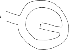
Figure 1: The RHS of (47), $C_{ik}{}^{l}C_{lt}{}^{k}$, is shown in this figure.

We call it a closed string metric. From (46) with the orthogonality relation of representations (A.1), we also have

$$\eta_{ij}=tr^{(r)}([\sigma_{i}][\sigma_{j}]),$$ (48)

where $[\sigma]$ is defined in (1). We can easily check that the closed string propagator is a projection operator

$$\eta_{i}{}^{j}\eta_{j}{}^{k}=\eta_{i}{}^{k},$$ (49)

where indices are raised by the open string metric,

$$\eta_{i}{}^{j}=g^{jk}\eta_{ik}.$$ (50)

The open string metric (38) secures the topological property of the closed string theory. In this way we obtain a topological closed string theory from the topological open string theory. The topological closed string theory is described by the centre of $\mathbb{C}[S_{n}]$ with the bilinear form $\eta_{ij}$. This Frobenius algebra is indeed what we have introduced in the previous section, which we denoted by ($Z(\mathbb{C}[S_{n}])$, $\eta$), if we ignore the $\Omega_{n}$ by taking a large $N$ limit.

For convenience, let us introduce a map from $\mathbb{C}[S_{n}]$ to $Z(\mathbb{C}[S_{n}])$ by

$$\pi(\sigma)=\sum_{i}\sigma_{i}\sigma\sigma^{i}=[\sigma].$$ (51)

From this definition it follows $\pi^{2}=\pi$. This gives a map from the open string states to the closed string states [8]. We can also define the map in terms of the the closed string propagator as

$$\eta_{i}{}^{j}\sigma_{j}=[\sigma_{i}].$$ (52)

Here we stress that the $\eta$ is a projector onto the centre of the group algebra $\mathbb{C}[S_{n}]$,

$$\eta_{i}{}^{j}[\sigma_{j}]=[\sigma_{i}].$$ (53)

Using the map we have

$$\eta_{ij}=tr^{(r)}(\pi(\sigma_{i})\pi(\sigma_{j}))=tr^{(r)}(\sigma_{i}\pi(\sigma_{j})),$$ (54)

where $\pi$ looks like a closed string mode propagating between two open string states (see figure 2). The property $\eta^{2}=\eta$ can be derived from $\pi^{2}=\pi$. The action of $\pi$ is diagonalised by the representation basis

$$\pi(P^{R})=P^{R}.$$ (55)

Closed string states are labelled by a Young diagram.

Starting with the noncommutative Frobenius algebra $(\mathbb{C}[S_{n}],g)$, the commutative Frobenius algebra also $(Z(\mathbb{C}[S_{n}]),\eta)$ comes in the game. We call this theory an open-closed topological theory. An axiomatic description of open-closed topological field theories was given in [21, 8].

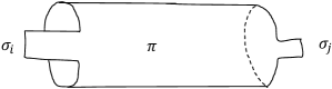
Figure 2: equaiton (54) is graphycally shown

We have explicitly reviewed the topological theory description of the group algebra obtained from the symmetric group, and the construction works for any semi-simple algebras [4, 3]. In [14] we have discussed topological field theories obtained from walled Brauer algebras.

5 Frobenius algebras with restricted structure

In the previous section we have reviewed that starting with a noncommutative Frobenius algebra with the Frobenius pairing (38), a commutative Frobenius algebra is uniquely obtained via (47), which is considered as the open-closed duality. In this section we will study Frobenius algebras associated with the algebras $\mathbb{C}[S_{n}]_{H}$ in more detail. Because these algebras are noncommutative, we are tempted to interpret these theories as open string theories. We will explore some aspects of the theories from the view point of the open-closed duality.

Recall that a basis of the algebra $\mathbb{C}[S_{n}]_{H}$ is spanned by

$$[\sigma]_{H}=\frac{1}{m!n!}\sum_{h\in H}h\sigma h^{-1},$$ (56)

which satisfy (7)-(8). Let $\Xi_{ij}{}^{k}$ be the structure constant of the algebra,

$$[\sigma_{i}]_{H}[\sigma_{j}]_{H}=\Xi_{ij}{}^{k}[\sigma_{k}]_{H}.$$ (57)

This is a noncommutative algebra

$$\Xi_{ij}{}^{k}\neq\Xi_{ji}{}^{k}.$$ (58)

In general the there are several choices for the Frobenius pairing. As we discussed in the last section, one possible Frobenius pairing for the noncommutative algebra is to use the prescription (38) as

$$G_{ij}=\Xi_{ik}{}^{l}\Xi_{jl}{}^{k}.$$ (59)

We call this noncommutative Frobenius algebra ($\mathbb{C}[S_{m+n}]_{H}$, $G$). The open-closed duality (47) gives a topological closed string theory described by the commutative Frobenius algebra. We construct it explicitly in appendix C.

On the other hand, it is also natural for us to use the two-point function as a Frobenius pairing of $\mathbb{C}[S_{m+n}]_{H}$. For example when $H=S\times S_{n}$, it is given by

$$\theta_{ij}=tr^{(r)}([\sigma_{i}]_{H}[\sigma_{j}]_{H}),$$ (60)

where we have ignored $\Omega_{m+n}$ to make this discussion simple. We will interpret it as an open string propagator. (It may also be interpreted as a cylinder amplitude by considering a triangulation with some links restricted in the subgroup [13, 14].) In section 3 this Frobenius algebra was called ($\mathbb{C}[S_{m+n}]_{H}$, $\theta$). A difference between these two Frobenius algebras, ($\mathbb{C}[S_{m+n}]_{H}$, $G$) and ($\mathbb{C}[S_{m+n}]_{H}$, $\theta$), is that $G_{ij}$ is written in terms of $\Xi$ as (59), while $\theta_{ij}$ does not satisfy $\Xi_{ik}{}^{l}\Xi_{jl}{}^{k}=\theta_{ij}$. This means that the propagator of the closed string theory dual to ($\mathbb{C}[S_{m+n}]_{H}$, $\theta$) does not have to be a projector. The relation between $G$ and $\theta$ will be shown in appendix C.

When $H=S_{n/2}[S_{2}]$, Frobenius algebra ($\mathbb{C}[S_{m+n}]_{H}$, $\varphi$) can be naturally considered, where

$$\varphi_{ij}=\frac{1}{N_{f}^{n/2}}\sum_{\rho\in S_{n}}W(\rho)tr^{(r)}([\sigma_{i}]_{H}\rho[\sigma_{j}]_{H}\rho^{-1}).$$ (63)

5.1 Noncommutative Frobenius algebra ($\mathbb{C}[S_{m+n}]_{S_{m}\times S_{n}}$, $\theta$)

In this subsection we consider the Frobenius algebra $(\mathbb{C}[S_{m+n}]_{H}$, $\theta$) for $H=S_{m}\times S_{n}$.

The indices of the open string metric $\theta_{ij}$ can be raised by $g^{ij}$ [14] as

$$\theta_{i}{}^{j}=tr^{(r)}([\sigma_{i}]_{H}[\sigma^{j}]_{H}),\quad\theta^{ij}=tr^{(r)}([\sigma^{i}]_{H}[\sigma^{j}]_{H}),$$ (64)

which satisfy $\theta_{ij}\theta^{jk}=\theta_{i}{}^{k}$. It has another expression

$$\theta_{i}{}^{j}=\sum_{R,A,\mu\nu}\frac{d^{R}}{d_{A}}\chi^{R}_{A,\mu\nu}(\sigma_{i})\chi^{R}_{A,\nu\mu}(\sigma^{j}).$$ (65)

Note that $\sum_{i}\theta_{i}{}^{i}=\sum_{R,A}(M^{R}_{A})^{2}$ counts the dimension of the vector space, i.e. the number of independent operators expressed by the form $P^{R}_{A,\mu\nu}$. Some partition functions of this theory were computed in [14] with a different interpretation from here.

The dual basis is defined in terms of the open string metric as

$$[\sigma^{k}]_{H}=\theta^{kl}[\sigma_{l}]_{H},$$ (66)

which is also the same as

$$[\sigma^{k}]_{H}=[g^{kl}\sigma_{l}]_{H}.$$ (67)

Closed string operators can be defined by generalising (51) to

$$\Pi([\sigma]_{H}):=\sum_{k}[\sigma_{k}]_{H}[\sigma]_{H}[\sigma^{k}]_{H}.$$ (68)

(Another way of defining closed string operators is to use (80).) They belong to the centre $Z(\mathbb{C}[S_{m+n}]_{H})$,

$$[\sigma]_{H}\Pi([\tau]_{H})=\Pi([\tau]_{H})[\sigma]_{H}.$$ (70)

This property is manifest in the form

$$\Pi([\sigma]_{H})=\sum_{R,A}\frac{1}{(d_{A})^{2}d_{R}}\chi^{R}_{A}(\sigma)P^{R}_{A}.$$ (71)

It is found that $\Pi^{2}$ is not equal to $\Pi$ due to an extra factor in the following, but it is still in the centre

$$\Pi(\Pi([\sigma_{i}]_{H}))=\sum_{R,A}\frac{e^{t_{R,A}}}{(d_{A})^{2}d_{R}}\chi^{R}_{A}(\sigma_{i})P^{R}_{A}.$$ (72)

where we have defined for our convenience

$$e^{t_{R,A}}:=\frac{M^{R}_{A}}{d_{A}d_{R}}.$$ (73)

It will be regarded as an area of a closed string cylinder. Inverting (71), central elements in the representation basis can be expanded as

$$P^{R}_{A}= \frac{d_{R}}{(m+n)!}e^{-t_{R,A}}\sum_{\sigma\in S_{m+n}}\chi^{R}_{A}(\sigma^{-1})\Pi([\sigma]_{H})$$ (74)

$$= d_{R}e^{-t_{R,A}}\sum_{i}\chi^{R}_{A}(\sigma^{i})\Pi([\sigma_{i}]_{H}).$$ (75)

We now compute the closed string propagator via the open-closed duality as

$$Z_{ij}=\Xi_{ik}{}^{l}\Xi_{lj}{}^{k}=tr^{(r)}([\sigma_{j}]_{H}\Pi([\sigma_{i}]_{H})).$$ (76)

It also takes the following form [14]

$$Z_{ij}=\sum_{R,A,\mu,\nu}\frac{1}{(d_{A})^{2}}\chi^{R}_{A,\mu\mu}(\sigma_{i})\chi^{R}_{A,\nu\nu}(\sigma_{j}).$$ (77)

Using the open string metric $\theta$, we define

$$Z_{i}{}^{l}=Z_{ij}\theta^{jl}=tr^{(r)}([\sigma^{l}]_{H}\Pi([\sigma_{i}]_{H})),$$ (78)

and $Z^{ij}$ is defined by $Z^{ij}=\theta^{ik}\theta^{jl}Z_{kl}$. These are consistent with $Z_{ij}Z^{jk}=Z_{i}{}^{k}$, but $Z_{i}{}^{k}$ does not satisfy $Z_{i}{}^{l}Z_{l}{}^{j}=Z_{i}{}^{j}$. In fact it can be shown that

$$Z_{i}{}^{l}Z_{l}{}^{j}=tr^{(r)}(\Pi([\sigma_{i}]_{H})\Pi([\sigma^{j}]_{H}))=tr^{(r)}([\sigma_{i}]_{H}\Pi^{2}([\sigma^{j}]_{H})),$$ (79)

which is not equal to $Z_{i}{}^{j}$ because of $\Pi^{2}\neq\Pi$.

Closed string states can be generated from open string states by acting with $Z_{i}{}^{l}$, which is a map onto the centre of the algebra,

$$Z_{i}{}^{l}[\sigma_{l}]_{H}=\Pi([\sigma_{i}]_{H}).$$ (80)

The $\Pi$ is diagonalised by the representation basis,

$$\Pi(P^{R}_{A,\mu\nu})=\delta_{\mu\nu}\frac{1}{d_{A}d_{R}}P^{R}_{A}.$$ (81)

In particular the eigenvalue of $\Pi^{n}:=(\Pi)^{n}$ is given by

$$\Pi^{n}(P^{R}_{A})=e^{nt_{RA}}P^{R}_{A}.$$ (82)

Here $t_{R,A}$ might be considered to be a parameter to measure the area of a closed string propagator [21]. The area depends on the set of representations $(R,A)$. Some partition functions of this closed string theory can be computed. For example, a torus amplitude is given by

$$Z_{ij}\theta^{ij}=\sum_{R,A}e^{t_{R,A}},$$ (84)

and another torus can be computed by

$$Z_{ij}Z^{ij}=\sum_{R,A}(e^{t_{R,A}})^{2}.$$ (85)

Some representations give the zero eigenvalue $t_{R,A}=0$. Irreducible representations of $H=S_{m}\times S_{n}$ are labelled by a set of two Young diagrams $A=(\alpha,\beta)$, where $\alpha$ is a Young diagram with $m$ boxes and $\beta$ is a Young diagram with $n$ boxes. The number of times the $A$ appears in $R$ is given by the Littlewood-Richardson coefficient, $M^{R}_{A}=g(\alpha,\beta;R)$. When both $R$ and $A$ are the symmetric representations $R=[m+n]$, $A=([m],[n])$, or both $R$ and $A$ are the anti-symmetric representations $R=[1^{m+n}]$, $A=([1^{m}],[1^{n}])$, we have an zero eigenvalue $t_{R,A}=0$. But for most representations we have $t_{R,A}\neq 0$.

Based on Brauer algebras open-closed systems can also be constructed very similarly following [14].

5.2 Noncommutative Frobenius algebra ($\mathbb{C}[S_{n}]_{S_{n/2}[S_{2}]}$, $\varphi$)

For the noncommutative algebra $\mathbb{C}[S_{n}]_{S_{n/2}[S_{2}]}$, as we discussed in section 3, it is interesting to consider the following bilinear form,

$$\varphi_{ij}=\frac{1}{N_{f}^{n/2}}\sum_{\rho\in S_{n}}W(\rho)tr^{(r)}([\sigma_{i}]_{H}\rho[\sigma_{j}]_{H}\rho^{-1})$$

$$\varphi^{ij}=\frac{1}{N_{f}^{n/2}}\sum_{\rho\in S_{n}}W(\rho)tr^{(r)}([\sigma^{i}]_{H}\rho[\sigma^{j}]_{H}\rho^{-1})$$

$$\varphi_{i}{}^{j}=\frac{1}{N_{f}^{n/2}}\sum_{\rho\in S_{n}}W(\rho)tr^{(r)}([\sigma_{i}]_{H}\rho[\sigma^{j}]_{H}\rho^{-1}),$$ (87)

which satisfy $\varphi_{ij}\varphi^{jk}=\varphi_{i}{}^{k}$. The commutative algebra arising from the centre of the noncommutative algebra $\mathbb{C}[S_{n}]_{S_{n/2}[S_{2}]}$ can be associated with a topological closed string theory in the same manner as the last subsection.

6 Summary

Based on the relationship between Frobenius algebras and two-dimensional topological field theories, we have discussed some aspects of the open-closed duality for Frobenius algebras that are related to the description of gauge invariant operators of ${\cal N}=4$ Super Yang-Mills.

We have focused on the the group algeba of symmetric group over the complex numbers. Considering the conjugacy classes leads to an associative algeba spanned by the central elements, which can be associated with gauge invariant operators built from one kind of complex scalar in ${\cal N}=4$ Super Yang-Mills. An interesting class of algebras can be introduced by considering equivalence relations using elements in subgroups of the symmetric group. The class of algebras were originally introduced to label gauge invariant operators in more general sectors than the one-complex scalar sector in ${\cal N}=4$ Super Yang-Mills. These algebras are associative and noncommutative. These noncommutative algebras can be interpreted as topological open string theories based on the equivalence between Frobenius algebras and two-dimensional topological field theories. We have associated two-point functions of ${\cal N}=4$ Super Yang-Mills with the bilinear form of the Frobenius algebras. It has been concretely observed that closed string degrees of freedom come out from the centre of the noncommutative algebras. The closed string states are labelled by a set of representations. It would be interesting to consider how the representations are interpreted in this context.

Acknowledgements

This work was supported by JSPS KAKENHI Grant Number 15K17673. We acknowledge useful conversations with Pablo Diaz, Robert de Mello Koch, Hai Lin, Sanjaye Ramgoolam, Ryo Suzuki at the ESF and STFC supported workshop “Permutations and Gauge String duality” in 2014.

Appendix A Useful formulas

Let $D^{R}_{ij}(\sigma)$ be a representation matrix of $\sigma\in S_{n}$. The orthogonality relation is given by

$$\frac{1}{n!}\sum_{\sigma\in S_{n}}D^{R}_{ij}(\sigma)D^{S}_{kl}(\sigma^{-1})=\frac{1}{d_{R}}\delta_{il}\delta_{jk}\delta_{RS},$$ (A.1)

where $d_{R}$ is the dimension of an irreducible representation $R$ of $S_{n}$.

The dimension of an irreducible representation $R$ of $U(N)$ can be expressed in terms of the Omega factor (27) as

$$DimR=\frac{N^{n}}{n!}\chi_{R}(\Omega_{n}),$$ (A.2)

where $\chi_{R}$ is the character of a representation $R$.

Appendix B Dual basis and the bilinear form

In this section, we give a supplementary explanation about the relationship between the bilinear form and the dual basis.

In order to make this discussion general, consider an associative algebra, where we denote elements of the algebra by $\phi_{i}$, the structure constants by $C_{ij}{}^{k}$. Here we will study the implication of the bilinear form determined by [4, 3]

$$g_{ij}=C_{ik}{}^{l}C_{jl}{}^{k}.$$ (B.1)

This makes the associative algebra Frobenius. The right-hand side represents the planar one-loop two-point function with the assignment of a 3pt-vertex to the structure constant.

Multiplying the equation by $\phi^{j}$, the right-hand side gives

$$C_{ik}{}^{l}C_{jl}{}^{k}\phi^{j}=C_{ik}{}^{l}\phi_{l}\phi^{k}=\phi_{i}\phi_{k}\phi^{k},$$ (B.2)

while the left-hand side gives

$$g_{ij}\phi^{j}=\phi_{i}.$$ (B.3)

We then obtain

$$\sum_{k}\phi_{k}\phi^{k}=1.$$ (B.4)

The condition (B.1) is equivalent to choosing the dual basis satisfying (B.4).

The Frobenius algebras appeared in section 4 and Appendix C have the Frobenius form in (B.1). On the other hand, the bilinear form in the Frobenius algebras introduced in section 5 do not take the form (B.1).

We can find the following equation,

$$C_{ij}{}^{k}g_{k0}=g_{ij}.$$ (B.5)

This is always satisfied, and it is not a condition which determines the form of the metric. This just gives a consistency condition, while (B.1) is a non-trivial constraint on the form of the metric.

Appendix C Another Frobenius algebra from $\mathbb{C}[S_{m+n}]_{H}$

In this appendix, the noncommutative Frobenius algebra $(\mathbb{C}[S_{m+n}]_{H},G)$ will be studied, where $G$ is given in (59). We explicitly construct the commutative Frobenius algebra obtained from this noncommutative Frobenius algebra.

We now have the open string metric given by

$$G_{ij}=\Xi_{ik}{}^{l}\Xi_{jl}{}^{k}=\sum_{R,A,\mu,\nu}\frac{M^{R}_{A}}{(d_{A})^{2}}\chi^{R}_{A,\mu\nu}(\sigma_{i})\chi^{R}_{A,\nu\mu}(\sigma_{j}),$$ (C.1)

and we also have

$$G^{ij}=\sum_{R,A,\mu,\nu}\frac{M^{R}_{A}}{(d_{A})^{2}}\chi^{R}_{A,\mu\nu}(\tilde{\sigma}^{i})\chi^{R}_{A,\nu\mu}(\tilde{\sigma}^{j}),$$

$$G_{i}{}^{j}=\sum_{R,A,\mu,\nu}\frac{M^{R}_{A}}{(d_{A})^{2}}\chi^{R}_{A,\mu\nu}(\sigma_{i})\chi^{R}_{A,\nu\mu}(\tilde{\sigma}^{j}),$$ (C.2)

where the new dual basis has been introduced by

$$\tilde{\sigma}^{i}=G^{ij}\sigma_{j}.$$ (C.3)

They satisfy $G_{ij}G^{jk}=G_{i}{}^{k}$ and $G_{i}{}^{j}G_{j}{}^{k}=G_{i}{}^{k}$, and $\Xi_{ij}{}^{k}G_{k0}=G_{ij}$. The two dual bases are simply related by

$$\chi^{R}_{A,\mu\nu}(\tilde{\sigma}^{i})=e^{-t_{R,A}}\chi^{R}_{A,\mu\nu}(\sigma^{i}),$$ (C.4)

where we recall that $t_{R,A}$ was defined in (73). As is expected, we have

$$G_{i}{}^{j}\sigma_{j}=[\sigma_{i}]_{H}.$$ (C.5)

A closed string propagator was obtained in (76). Because indices of $Z_{ij}$ are raised by the open string metric $G^{ij}$, we introduce

$$\tilde{Z}_{i}{}^{j}:=Z_{ik}G^{kj}=\sum_{R,A,\mu,\nu}\frac{1}{(d_{A})^{2}}\chi^{R}_{A,\mu\mu}(\sigma_{i})\chi^{R}_{A,\nu\nu}(\tilde{\sigma}^{j}).$$ (C.6)

We can show $\tilde{Z}_{i}{}^{j}\tilde{Z}_{j}{}^{k}=\tilde{Z}_{i}{}^{k}$ as expected. Another consistency check is $\tilde{Z}_{ij}\tilde{Z}^{jk}=\tilde{Z}_{i}{}^{k}$, where

$$\tilde{Z}^{ij}:=Z_{kl}G^{ki}G^{lj}=\sum_{R,A,\mu,\nu}\frac{1}{(d_{A})^{2}}\chi^{R}_{A,\mu\mu}(\tilde{\sigma}^{i})\chi^{R}_{A,\nu\nu}(\tilde{\sigma}^{j}).$$ (C.7)

Similarly to (51) and (68), closed string states are defined by

$$\tilde{\Pi}(\sigma_{i})=[\sigma_{k}]_{H}[\sigma_{i}]_{H}[\tilde{\sigma}^{k}]_{H} =\sum_{R,A}\frac{1}{M^{R}_{A}d_{A}}\chi^{R}_{A}(\sigma_{i})P^{R}_{A}$$ (C.8)

or

$$\tilde{\Pi}(\sigma_{i})=\tilde{Z}_{i}{}^{j}[\sigma_{j}]_{H}.$$ (C.9)

The inverse transformation gives the expansion of central projectors in $Z(\mathbb{C}[S_{n}]_{H})$ as

$$P^{R}_{A}=d_{R}\sum_{i}\chi^{R}_{A}(\sigma^{i})\tilde{\Pi}(\sigma_{i}).$$ (C.10)

We find that $\tilde{\Pi}^{2}=\tilde{\Pi}$, and on the representation basis $\tilde{\Pi}$ is diagonalised by

$$\tilde{\Pi}(P^{R}_{A})=P^{R}_{A}.$$ (C.11)

From appendix B, we expect the dual basis introduced in this section should satisfies $\sum_{i}[\sigma_{i}]_{H}[\tilde{\sigma}^{i}]_{H}=1$, and it is the case:

$$\sum_{i}[\sigma_{i}]_{H}[\tilde{\sigma}^{i}]_{H}$$

$$= \sum_{i,j}[\sigma_{i}]_{H}[\sigma_{j}]_{H}G^{ij}$$

$$= \sum_{R,A,\mu\nu}\frac{1}{d_{A}}\chi^{R}_{A,\mu\nu}(\sigma_{i})P^{R}_{A,\mu\nu}\sum_{S,B,\alpha\beta}\frac{1}{d_{B}}\frac{d_{S}d_{B}}{M^{S}_{B}}\chi^{S}_{B,\alpha\beta}(\sigma^{i})P^{S}_{B,\alpha\beta}$$

$$= \sum_{R,A}P^{R}_{A}=1.$$ (C.12)

The trace part of $\tilde{Z}_{i}^{j}$ has a mathematical meaning. Because $\tilde{Z}_{i}^{j}$ is a projection operator onto the centre $Z(\mathbb{C}(S_{n})_{H})$, the trace part counts the dimension of the vector space,

$$\tilde{Z}_{i}{}^{i}=\sum_{R,A}\frac{M_{RA}}{M_{RA}}=\sum_{R,A}\delta_{M_{R,A},0}.$$ (C.13)

Indeed this coincides the number of the operators $P^{R}_{A}$.

Appendix D Another representation basis

In this appendix, we will study Frobenius algebra $(\mathbb{C}[S_{n}]_{H},\theta)$ in terms of a different representation basis introduced in [9, 13].

Let us introduce branching coefficients $B^{\Lambda\rightarrow 1_{H},\alpha}_{l}$ of an irreducible representation $\Lambda$ of $S_{n}$, where $l$ runs over $1,\cdots,d_{\Lambda}$. They are the quantities satisfying

$$\sum_{\alpha}B^{\Lambda\rightarrow 1_{H},\alpha}_{l_{1}}B^{\Lambda\rightarrow 1_{H},\alpha}_{l_{2}}=\frac{1}{|H|}\sum_{h\in H}D^{\Lambda}_{l_{1}l_{2}}(h)$$ (D.14)

and

$$\sum_{l}B^{\Lambda\rightarrow 1_{H},\alpha}_{l}B^{\Lambda\rightarrow 1_{H},\beta}_{l}=\delta_{\alpha\beta}.$$ (D.15)

Here the indices $\alpha,\beta$ run over $1,\cdots,M^{\Lambda}_{1_{H}}$, where $M^{\Lambda}_{1_{H}}$ is the number of times the singlet representation $1_{H}$ of $H$ appears in $\Lambda$. From the reality of the representation of $S_{n}$, we have $B^{\dagger}=B$.

Another important quantities are Clebsh-Gordan coefficients $S^{RS,\Lambda\tau}_{ab,l}$. Here $R,S,\Lambda$ are irreducible representations of $S_{n}$, and $a,b$ and $l$ run over $1,\cdots,d_{R}$, $1,\cdots,d_{S}$ and $1,\cdots,d_{\Lambda}$, respectively. $\tau$ is a multiplicity label counting the number of times $\Lambda$ appears in $R\otimes R$, running over $1,\cdots,C(R,S,\Lambda)$. For our convenience, we define

$$\tilde{S}^{RR,\Lambda\tau,\alpha}_{ab}:=\sum_{l}S^{RR,\Lambda\tau}_{ab,l}B^{\Lambda\rightarrow 1_{H},\alpha}_{l}.$$ (D.17)

In terms of these group theoretical quantities, we can show

$$[\sigma_{i}]_{H}=\sum_{R,\Lambda,\tau,\alpha,l}d_{R}D^{R}_{ab}(\sigma_{i})\tilde{S}^{RR,\Lambda\tau,\alpha}_{ab}P^{R,\Lambda,\tau,\alpha},$$ (D.21)

where

$$P^{R,\Lambda,\tau,\alpha} =\sum_{i}D^{R}_{ba}(\sigma^{i})\tilde{S}^{RR,\Lambda\tau,\alpha}_{ab}\sigma_{i}$$ (D.22)

$$=\sum_{i}D^{R}_{ba}(\sigma^{i})\tilde{S}^{RR,\Lambda\tau,\alpha}_{ab}[\sigma_{i}]_{H}.$$ (D.23)

When $H=S_{n/2}[S_{2}]$, the Branching coefficients are zero if $\Lambda$ is odd. If $\Lambda$ is even, $M^{\Lambda}_{1_{H}}=1$, so the index $\alpha$ is trivial;

$$P^{R,\Lambda,\tau} =\sum_{i}D^{R}_{ba}(\sigma^{i})S^{RR,\Lambda\tau}_{ab,l}B_{l}^{\Lambda\rightarrow 1_{H}}[\sigma_{i}]_{H}.$$ (D.24)

This property has played an important role in [15].

For later convenience we now express the noncommutativity of the algebra in the following way

$$P^{R\Lambda\tau\alpha}P^{R^{\prime}\Lambda^{\prime}\tau^{\prime}\alpha^{\prime}}$$ (D.25)

$$= \left(\sum_{i}D^{R}_{ab}(\sigma^{i})\tilde{S}^{RR,\Lambda\tau,\alpha}_{ba}\sigma_{i}\right)\left(\sum_{k}D^{R^{\prime}}_{cd}(\sigma^{k})\tilde{S}^{R^{\prime}R^{\prime},\Lambda^{\prime}\tau^{\prime},\alpha^{\prime}}_{dc}\sigma_{k}\right)$$

$$= \frac{1}{d_{R}}\delta_{RR^{\prime}}\sum_{i}D^{R}_{cb}(\sigma^{i})(\tilde{S}^{RR,\Lambda\tau,\alpha}\ast\tilde{S}^{R^{\prime}R^{\prime},\Lambda^{\prime}\tau^{\prime},\alpha^{\prime}})_{bc}\sigma_{i},$$

where we have defined

$$(\tilde{S}^{RR,\Lambda\tau,\alpha}\ast\tilde{S}^{R^{\prime}R^{\prime},\Lambda^{\prime}\tau^{\prime},\alpha^{\prime}})_{bc}=\tilde{S}^{RR,\Lambda\tau,\alpha}_{ba}\tilde{S}^{R^{\prime}R^{\prime},\Lambda^{\prime}\tau^{\prime},\alpha^{\prime}}_{ac}.$$ (D.26)

This non-commutative product is an analogue of $P^{R}_{A,\mu\nu}P^{S}_{B,\alpha\beta}=\delta_{\nu\alpha}\delta_{RS}\delta_{AB}P^{S}_{B,\mu\beta}$.

Defining

$$\hat{D}_{ab}^{R}:=d^{R}D^{R}_{ba}(\sigma^{i})\sigma_{i},$$ (D.27)

the product rule is the usual matrix product

$$\hat{D}^{R}_{ab}\hat{D}^{R^{\prime}}_{cd}=\delta_{bc}\delta^{RR^{\prime}}\hat{D}^{R}_{ad}.$$ (D.29)

With this notation we have

$$P^{R\Lambda\tau\alpha}=\frac{1}{d_{R}}\hat{D}^{R}_{ab}\tilde{S}^{RR,\Lambda\tau,\alpha}_{ab},$$ (D.30)

$$P^{RR,\Lambda\tau,\alpha}P^{R^{\prime}R^{\prime},\Lambda^{\prime}\tau^{\prime},\alpha^{\prime}}=\frac{1}{(d_{R})^{2}}\delta_{RR^{\prime}}\hat{D}^{R}_{ab}(\tilde{S}^{RR,\Lambda\tau,\alpha}\ast\tilde{S}^{R^{\prime}R^{\prime},\Lambda^{\prime}\tau^{\prime},\alpha^{\prime}})_{ab},$$ (D.31)

$$P^{R\Lambda\tau\alpha}P^{R^{\prime}\Lambda^{\prime}\tau^{\prime}\alpha^{\prime}}P^{R^{\prime\prime}\Lambda^{\prime\prime}\tau^{\prime\prime}\alpha^{\prime\prime}}$$

$$=\frac{1}{(d_{R})^{3}}\delta_{RR^{\prime}}\delta_{RR^{\prime\prime}}\hat{D}^{R}_{ab}(\tilde{S}^{RR,\Lambda\tau,\alpha}\ast\tilde{S}^{RR,\Lambda^{\prime}\tau^{\prime},\alpha^{\prime}}\ast\tilde{S}^{RR,\Lambda^{\prime\prime}\tau^{\prime\prime},\alpha^{\prime\prime}})_{ab}.$$ (D.32)

The closed string state can be calculated to be

$$\Pi([\sigma_{s}]_{H}) = \sum_{R,\Lambda,\tau,\alpha}\sum_{\Lambda^{\prime},\tau^{\prime},\alpha^{\prime}}\sum_{\Lambda^{\prime\prime},\tau^{\prime\prime},\alpha^{\prime\prime}}D^{R}_{cd}(\sigma_{s})\tilde{S}^{RR,\Lambda^{\prime}\tau^{\prime},\alpha^{\prime}}_{cd}(\tilde{S}^{RR,\Lambda\tau,\alpha}\ast\tilde{S}^{RR,\Lambda^{\prime\prime}\tau^{\prime\prime},\alpha^{\prime\prime}})_{ff}$$ (D.33)

$$\frac{1}{d_{R}}\hat{D}^{R}_{ab}(\tilde{S}^{RR,\Lambda\tau,\alpha}\ast\tilde{S}^{RR,\Lambda^{\prime}\tau^{\prime},\alpha^{\prime}}\ast\tilde{S}^{RR,\Lambda^{\prime\prime}\tau^{\prime\prime},\alpha^{\prime\prime}})_{ab}.$$

References

• [1] G. Segal, “The definition of conformal field theory.”
• [2] M. Atiyah, “Topological quantum field theories,” Inst. Hautes Etudes Sci. Publ. Math.  68 (1989) 175.
• [3] M. Fukuma, S. Hosono and H. Kawai, “Lattice topological field theory in two-dimensions,” Commun. Math. Phys.  161 (1994) 157 doi:10.1007/BF02099416 [hep-th/9212154].
• [4] C. Bachas and P. M. S. Petropoulos, “Topological models on the lattice and a remark on string theory cloning,” Commun. Math. Phys.  152 (1993) 191 doi:10.1007/BF02097063 [hep-th/9205031].
• [5] L. Abrams, “Two dimensional topological quantum field theories and Frobenius algebras,” J. Knot Theory and its Ramifications 5 (1996), 569-587.
• [6] J. Kock, “Frobenius algebras and 2D topological quantum field theories,” Cambridge University Press.
• [7] G. Segal, “Topological structures in string theory,” Phil. Trans. R. Soc. Lond. A (2001) 359, 1389.
• [8] G. W. Moore and G. Segal, “D-branes and K-theory in 2D topological field theory,” hep-th/0609042.
• [9] T. W. Brown, P. J. Heslop and S. Ramgoolam, “Diagonal multi-matrix correlators and BPS operators in N=4 SYM,” JHEP 0802 (2008) 030 doi:10.1088/1126-6708/2008/02/030 [arXiv:0711.0176 [hep-th]].
• [10] Y. Kimura and S. Ramgoolam, “Branes, anti-branes and brauer algebras in gauge-gravity duality,” JHEP 0711 (2007) 078 doi:10.1088/1126-6708/2007/11/078 [arXiv:0709.2158 [hep-th]].
• [11] R. Bhattacharyya, S. Collins and R. de Mello Koch, “Exact Multi-Matrix Correlators,” JHEP 0803 (2008) 044 doi:10.1088/1126-6708/2008/03/044 [arXiv:0801.2061 [hep-th]].
• [12] P. Mattioli and S. Ramgoolam, “Permutation Centralizer Algebras and Multi-Matrix Invariants,” Phys. Rev. D 93 (2016) no.6, 065040 doi:10.1103/PhysRevD.93.065040 [arXiv:1601.06086 [hep-th]].
• [13] J. Pasukonis and S. Ramgoolam, “Quivers as Calculators: Counting, Correlators and Riemann Surfaces,” JHEP 1304 (2013) 094 doi:10.1007/JHEP04(2013)094 [arXiv:1301.1980 [hep-th]].
• [14] Y. Kimura, “Multi-matrix models and Noncommutative Frobenius algebras obtained from symmetric groups and Brauer algebras,” Commun. Math. Phys.  337 (2015) no.1, 1 doi:10.1007/s00220-014-2231-6 [arXiv:1403.6572 [hep-th]].
• [15] Y. Kimura, S. Ramgoolam and R. Suzuki, “Flavour singlets in gauge theory as Permutations,” arXiv:1608.03188 [hep-th].
• [16] Y. Kimura, “Correlation functions and representation bases in free N=4 Super Yang-Mills,” Nucl. Phys. B 865 (2012) 568 doi:10.1016/j.nuclphysb.2012.08.010 [arXiv:1206.4844 [hep-th]].
• [17] V. Balasubramanian, D. Berenstein, B. Feng and M. x. Huang, “D-branes in Yang-Mills theory and emergent gauge symmetry,” JHEP 0503 (2005) 006 doi:10.1088/1126-6708/2005/03/006 [hep-th/0411205].
• [18] R. de Mello Koch, J. Smolic and M. Smolic, “Giant Gravitons - with Strings Attached (I),” JHEP 0706 (2007) 074 doi:10.1088/1126-6708/2007/06/074 [hep-th/0701066].
• [19] Y. Kimura and S. Ramgoolam, “Enhanced symmetries of gauge theory and resolving the spectrum of local operators,” Phys. Rev. D 78 (2008) 126003 doi:10.1103/PhysRevD.78.126003 [arXiv:0807.3696 [hep-th]].
• [20] S. Corley, A. Jevicki and S. Ramgoolam, “Exact correlators of giant gravitons from dual N=4 SYM theory,” Adv. Theor. Math. Phys.  5 (2002) 809 [hep-th/0111222].
• [21] G.  Segal, Lectures at Stanford University, 1999.
• [22] M. Hamermesh, “Group Theory and its Applications to Physical Problems,” Dover Publications.