Excitations and stability of weakly interacting Bose gases with multi-body interactions

Abstract

We consider weakly interacting bosonic gases with local and non-local multi-body interactions. By using the Bogoliubov approximation, we first investigate contact interactions, studying the case in which the interparticle potential can be written as a sum of $N$-body $\delta$-interactions, and then considering general contact potentials. Results for the quasi-particle spectrum and the stability are presented. We then examine non-local interactions, focusing on two different cases of $3$-body non-local interactions. Our results are used for systems with $2$- and $3$-body $\delta$-interactions and applied for realistic values of the trap parameters. Finally, the effect of conservative $3$-body terms in dipolar systems and soft-core potentials (that can be simulated with Rydberg dressed atoms) is also studied.

I Introduction

The Bogoliubov theory of weakly interacting Bose gases bogoliubov1947 provides an essential tool to investigate the effect of interactions in bosonic systems zagrebnov2001 and it plays a key role in the study of properties of Bose-Einstein condensates pethick2002 ; pitaevskii2016 . Its results for the ground-state energy and condensate depletion are in agreement in the weakly interacting limit with the findings obtained by other methods subsequently developed, including rigorous treatments lieb2005 . An important point is that also when it does not (quantitatively) work, it is useful to have results which are of guide for a qualitative understanding, as in the case of Helium$4$ annett2004 ; pitaevskii2016 , or to have estimates of the ground-state energy, as in the case of the $1D$ Lieb-Liniger model for small couplings lieb1961 . Moreover, being a self-consistent approach, where the number of condensate particles has to be self-consistently determined, it gives information on the issue whether there is condensation or not, as in low-dimensional systems pethick2002 ; pitaevskii2016 . Finally, the Bogoliubov transformation used to diagonalize the quadratic Hamiltonian obtained by the Bogoliubov approximation is used in a variety of other systems, including spin-wave theory of antiferromagnets manousakis1991 and superconductors schrieffer1964 ; bogoliubov1959 .

In this paper we study the generalization of the Bogoliubov theory to local and non-local/finite-range $3$-body and general multi-body interactions. Our reasons for such an investigation are the following:

• We are firstly motivated by the the interest in studying the effects that the presence of $3$-body terms in experiments with ultracold atoms may induce on their equilibrium and dynamical properties, including the quasi-particle spectrum, with the goal to quantify how large are such effects.

• More generally, when (local or non-local/finite-range) $2$-body terms are present jointly with higher-body contributions (as $3$-body ones), they may compete to make the system stable or unstable and it is of interest to determine stability conditions and the spectrum of the quasi-particles. A typical example is given by an attractively interacting Bose gas, having $a<0$, which can be made stable by a repulsive $3$-body term.

• Another motivation is provided by the dipolar gas in presence of a $3$-body term xi16 ; bisset15 . The effect of $3$-body interaction terms in dipolar systems can be very interesting. As an example, it was recently shown that for a harmonically trapped dilute dipolar condensate with a $3$-body short-range interaction the system exhibits a condensate state and a droplet state blakie2016 , discussing how the droplet crystal may be an excited state arising from heating as the system crosses the phase transition. In the following we derive within the Bogoliubov theory the stability condition in presence of general multi-body local interactions (considering the case of $3$-body non-local interactions as well), then we discuss in detail some specific examples.

• A tool to study ultracold strongly interacting systems such as $1$D Bose gas lieb1961 or unitary Fermi gases zwerger2012 is to introduce effective local interactions. Recent examples are provided by the recent study of the monopole excitations for the $1$D Bose gas choi2015 using an effective Gross-Pitaevskii equation of the form

  $$i\hbar\frac{\partial\psi}{\partial t}=-\frac{\hbar^{2}}{2m}\nabla^{2}\psi+V_{ext}\psi+f(\rho)\psi\mbox{,}$$ (1)

  where $V_{ext}$ is the external potential, $\rho=\mid\psi\mid^{2}$ is the density and the non-linear term $f(\rho)$ is extracted from the solution of the Bethe ansatz integral equations for the (homogeneous) $1D$ Bose gas lieb1961 ; yang1969 . Another example is the study of small-amplitude Josephson oscillations of a ⁶Li unitary Fermi gas in a double well potential valtolina2015 , where experimental data were compared with an equation of the form (1) with $\rho$ the pair density, $V_{ext}$ the double well one-body potential and $f(\rho)$ extracted from Monte Carlo numerical results valtolina2015 (an example of a possible parametrization of $f(\rho)$ across the BEC-BCS crossover is in manini2005 ). It is clear that in the weakly interacting limit it is $f(\rho)\propto\rho$: this corresponds for the $1D$ Bose gas to the limit $\gamma\to 0$, where $\gamma$ is the Lieb-Liniger coupling constant lieb1961 , and for fermions in the BEC-BCS crossover to the BEC limit $a\to 0^{+}$, $a$ being the scattering length. When deviations from the weakly interacting limit are incorporated through a function $f$ which is no longer proportional to $\rho$, if the function $f$ admits a series expansion of the form $f=\sum_{n}c_{n}\rho^{n}$, then there are effective multi-body local interactions (corresponding to integer values $n\geq 2$). Therefore, to treat such multi-body (albeit effective) interaction terms one needs to study in the Bogoliubov theory such higher-body terms, as we do systematically below.

The paper is organized as follows. In Section II we consider general multi-body contact interactions for a homogeneous weakly interacting gas treated in the Bogoliubov approximation. We consider first the case of an $N$-body $\delta$-interaction and successively we consider a local interaction which can be expanded in series of general $N$-body terms. For this class of interactions we compute the spectrum, the stability condition and the ground-state energy (also for the $1D$ case). We finally present results for contact interactions that cannot be expanded in series. In Section III we discuss the case of non-local interactions: after briefly reviewing the well-known case of a $2$-body non-local interaction, we study two different cases of $3$-body non-local interactions, and a comparison between these two cases is performed with a Gaussian pair-wise interaction. The results of Sections II and III are used in Section IV in the case of a model with $2$- and $3$-body contact interactions and the obtained findings are applied to possible realistic values of the trap parameters. In Section V we discuss some further realistic interaction potentials of interest for current experimental setups with ultracold atoms. We present results for a $2$-body non-local potential plus $2$- and $3$-body $\delta$-interactions, with applications to dipolar systems, e.g. magnetic atoms and polar molecules, and soft-core potentials, that can be simulated with Rydberg dressed atoms, to discuss the effect of a $3$-body interaction term. Finally we present our conclusions in Section VI, while more technical material is presented in the Appendices.

II Contact interactions

In this Section we consider general local $\delta$-interparticle potentials with multi-body interactions.

II.1 $N$-body interaction

We start by considering a model for a gas of $N_{T}$ bosonic particles interacting only via local repulsive $N$-body $\delta$-interactions.

The general Hamiltonian for $N$-body interactions reads

$$\hat{H}=\int\!\mathrm{d}\mathbf{r}\,\hat{\Psi}^{\dagger}(\mathbf{r})\,\biggl{(}-\frac{\hbar^{2}\nabla^{2}}{2m}\biggr{)}\,\hat{\Psi}(\mathbf{r})+\frac{1}{N!}\int\!\mathrm{d}\mathbf{r}_{1}\cdots\mathrm{d}\mathbf{r}_{N}\,\hat{\Psi}^{\dagger}(\mathbf{r}_{1})\cdots\hat{\Psi}^{\dagger}(\mathbf{r}_{N})\,U(\mathbf{r}_{1},\ldots,\mathbf{r}_{N})\,\hat{\Psi}(\mathbf{r}_{N})\cdots\hat{\Psi}(\mathbf{r}_{1})\mbox{,}$$ (2)

where the bosonic field operators satisfy the canonical commutation relations $\left[\hat{\Psi}(\mathbf{r}),\hat{\Psi}(\mathbf{r^{\prime}})\right]=0=\left[\hat{\Psi}^{\dagger}(\mathbf{r}),\hat{\Psi}^{\dagger}(\mathbf{r^{\prime}})\right]$ and $\left[\hat{\Psi}(\mathbf{r}),\hat{\Psi}^{\dagger}(\mathbf{r^{\prime}})\right]=\delta(\mathbf{r}-\mathbf{r^{\prime}})$. We assume $N$-body local contact interactions having the form:

$$U(\mathbf{r}_{1},\ldots,\mathbf{r}_{N})\equiv U_{N}\prod_{\begin{subarray}{c}i<j\end{subarray}}\delta(\mathbf{r}_{i}-\mathbf{r}_{j})\mbox{,}$$ (3)

where $U_{N}$ is a coefficient of dimension $[U_{N}]=[E]\cdot[L]^{3N-3}$. In the usual case of 2-body $\delta$-interaction one has $U_{2}=\frac{4\pi\hbar^{2}a}{m}$, where $m$ is the mass of the bosons pethick2002 ; pitaevskii2016 . With potential (3) the Hamiltonian reads

$$\hat{H}=\int\!\mathrm{d}\mathbf{r}\,\hat{\Psi}^{\dagger}(\mathbf{r})\,\biggl{(}-\frac{\hbar^{2}\nabla^{2}}{2m}\biggr{)}\,\hat{\Psi}(\mathbf{r})+\frac{U_{N}}{N!}\int\!\mathrm{d}\mathbf{r}\,\biggl{(}\hat{\Psi}^{\dagger}(\mathbf{r})\biggr{)}^{\!N}\!\!\!\cdot\!\biggl{(}\hat{\Psi}(\mathbf{r})\biggr{)}^{\!N}\mbox{.}$$ (4)

Using for the field operator the expansion

$$\hat{\Psi}(\mathbf{r})=\sum_{\mathbf{p}}{\Psi}_{\mathbf{p}}(\mathbf{r})\,\hat{a}_{\mathbf{p}}\mbox{,}$$ (5)

where $\Omega=L^{3}$ is the volume of the system (chosen to be a cube of side $L$ with periodic boundary conditions) and ${\Psi}_{\mathbf{p}}(\mathbf{r})=\frac{1}{\sqrt{\Omega}}e^{i\mathbf{k}\cdot\mathbf{r}}$, with $\mathbf{p}=\hbar\mathbf{k}$, the Hamiltonian assumes the form

$$\hat{H}=\hat{H_{0}}+\hat{H}_{I}\mbox{,}$$ (6)

with $\hat{H_{0}}$ given as usual by

$$\hat{H}_{0}=\sum_{\mathbf{p}}\epsilon_{p}^{0}\,\hat{a}_{\mathbf{p}}^{\dagger}\hat{a}_{\mathbf{p}}\mbox{,}$$ (7)

where $\epsilon_{p}^{0}=p^{2}/2m$, and the interaction part reading as

$$\hat{H}_{I}=\frac{U_{N}}{\Omega^{N-1}N!}\!\sum_{\bigl{(}\sum_{i}\mathbf{p}_{i}=\sum_{i}\mathbf{p}_{i}^{\prime}\bigr{)}}\!\!\!\!\!\hat{a}_{\mathbf{p}_{1}^{\prime}}^{\dagger}\cdots\hat{a}_{\mathbf{p}_{N}^{\prime}}^{\dagger}\hat{a}_{\mathbf{p}_{N}}\cdots\hat{a}_{\mathbf{p}_{1}}\mbox{,}$$ (8)

with the definition

$$\sum_{\bigl{(}\sum_{i}\mathbf{p}_{i}=\sum_{i}\mathbf{p}_{i}^{\prime}\bigr{)}}\!\equiv\sum_{\begin{subarray}{c}\mathbf{p}_{1},\ldots,\mathbf{p}_{N}\\ \mathbf{p}_{1}^{\prime},\ldots,\mathbf{p}_{N}^{\prime}\end{subarray}}\!\!\delta_{\mathbf{p}_{1}+\ldots+\mathbf{p}_{N},\,\mathbf{p}_{1}^{\prime}+\ldots+\mathbf{p}_{N}^{\prime}}\mbox{.}$$ (9)

Now, proceeding as usual, we make the Bogoliubov prescription bogoliubov1947 ; zagrebnov2001

$$\hat{a}_{0}\sim\sqrt{N_{0}}\mbox{.}$$

As usual this implies that $N_{0}\sim N_{T}$, where $N_{0}$ is the condensate number, or the largest eigenvalue of the one-body density matrix pitaevskii2016 . We then proceed by neglecting in $\hat{H}_{I}$ products of 3 or more $\hat{a}_{\mathbf{p}}^{\dagger}$ with $\mathbf{p}\neq 0$.

To start with, we consider $3$-body interactions, that is, $N=3$. From (9) it follows the total momentum conservation. Therefore, one has to arrange $2$ nonzero momenta between $3$ initial and $3$ final possible momenta. To enumerate all the possibilities, we may start by considering all the momenta of the creation operators equal to zero:

$\mathbf{p}_{1}^{\prime}$	$\mathbf{p}_{2}^{\prime}$	$\mathbf{p}_{3}^{\prime}$	$\mathbf{p}_{1}$	$\mathbf{p}_{2}$	$\mathbf{p}_{3}$
0	0	0	0	$\mathbf{p}$	$-\mathbf{p}$
			$\mathbf{p}$	0	$-\mathbf{p}$
			$\mathbf{p}$	$-\mathbf{p}$	0

i.e. the contribution to $\hat{H}_{I}$ is $N_{0}^{2}\,\hat{a}_{\mathbf{p}}\hat{a}_{-\mathbf{p}}$ multiplied by $3$, that is the combinatorial multiplicity, $3=\binom{3}{2}$, as illustrated in the table above. For a generic $N$, it is therefore straightforward to conclude that the coefficient $\binom{3}{2}$ has to be replaced by $\binom{N}{2}$.

Going ahead, the next possible arrangements are

$\mathbf{p}_{1}^{\prime}$	$\mathbf{p}_{2}^{\prime}$	$\mathbf{p}_{3}^{\prime}$	$\mathbf{p}_{1}$	$\mathbf{p}_{2}$	$\mathbf{p}_{3}$
$\mathbf{p}$	0	0	$\mathbf{p}$	0	0
			0	$\mathbf{p}$	0
			0	0	$\mathbf{p}$
0	$\mathbf{p}$	0	$\mathbf{p}$	0	0
			0	$\mathbf{p}$	0
			0	0	$\mathbf{p}$
0	0	$\mathbf{p}$	$\mathbf{p}$	0	0
			0	$\mathbf{p}$	0
			0	0	$\mathbf{p}$

from which one can infer that the corresponding contribution to $\hat{H}_{I}$ is $N_{0}^{2}\,\hat{a}_{\mathbf{p}}^{\dagger}\hat{a}_{\mathbf{p}}$ with multiplicity $9$. For a general $N$ the multiplicity is $N^{2}$.

Finally, the remaining possibilities are when all the momenta of the annihilation operators are vanishing:

$\mathbf{p}_{1}^{\prime}$	$\mathbf{p}_{2}^{\prime}$	$\mathbf{p}_{3}^{\prime}$	$\mathbf{p}_{1}$	$\mathbf{p}_{2}$	$\mathbf{p}_{3}$
$\mathbf{p}$	$-\mathbf{p}$	0	0	0	0
$\mathbf{p}$	0	$-\mathbf{p}$
0	$\mathbf{p}$	$-\mathbf{p}$

whose contribution to the operatorial part is $N_{0}^{2}\,\hat{a}_{\mathbf{p}}^{\dagger}\hat{a}_{-\mathbf{p}}^{\dagger}$ with multiplicity 3, as in the first case considered above; hence, for a general $N$, the multiplicity is $\binom{N}{2}$.

Thus, the Hamiltonian (6) in the Bogoliubov approximation for a general $N$ reads

$$\hat{H}=\sum_{\mathbf{p}\neq 0}\epsilon_{p}^{0}\,\hat{a}_{\mathbf{p}}^{\dagger}\hat{a}_{\mathbf{p}}+\frac{U_{N}}{\Omega^{N-1}N!}\bigl{(}\sqrt{N_{0}}\bigr{)}^{2N}\!+\frac{U_{N}}{\Omega^{N-1}N!}\bigl{(}\sqrt{N_{0}}\bigr{)}^{2N-2}\sum_{\mathbf{p}\neq 0}\biggl{\{}\binom{N}{2}\bigl{(}\hat{a}_{\mathbf{p}}\hat{a}_{-\mathbf{p}}+\hat{a}_{\mathbf{p}}^{\dagger}\hat{a}_{-\mathbf{p}}^{\dagger}\bigr{)}+N^{2}\,\hat{a}_{\mathbf{p}}^{\dagger}\hat{a}_{\mathbf{p}}\biggr{\}}\mbox{.}$$ (10)

Defining the density $n\equiv\frac{N_{T}}{\Omega}$ and the condensate fraction $n_{0}\equiv\frac{N_{0}}{\Omega}$, one gets

$$\hat{H}=\frac{U_{N}N_{0}^{N}}{\Omega^{N-1}N!}+\sum_{\mathbf{p}\neq 0}\biggl{[}\epsilon_{p}^{0}+U_{N}n_{0}^{N-1}\frac{N^{2}}{N!}\biggr{]}\hat{a}_{\mathbf{p}}^{\dagger}\hat{a}_{\mathbf{p}}+U_{N}n_{0}^{N-1}\frac{N(N-1)}{2N!}\sum_{\mathbf{p}\neq 0}\biggl{[}\hat{a}_{\mathbf{p}}^{\dagger}\hat{a}_{-\mathbf{p}}^{\dagger}+\hat{a}_{\mathbf{p}}\hat{a}_{-\mathbf{p}}\biggr{]}\mbox{.}$$ (11)

Introducing the total particle number operator

$$\hat{N}=\sum_{\mathbf{p}}\hat{a}_{\mathbf{p}}^{\dagger}\hat{a}_{\mathbf{p}}\mbox{,}$$ (12)

and enforcing the total number conservation (or, in other terms, subtracting the chemical potential pethick2002 ), one finally obtains

$$\hat{H}=\frac{U_{N}n^{N-1}}{N!}N_{T}+\sum_{\mathbf{p}\neq 0}\Biggl{(}\epsilon_{p}^{0}+\frac{N(N\!-\!1)}{N!}U_{N}n_{0}^{N-1}\Biggr{)}\hat{a}_{\mathbf{p}}^{\dagger}\hat{a}_{\mathbf{p}}+\sum_{\mathbf{p}\neq 0}\frac{N(N\!-\!1)}{2N!}U_{N}n_{0}^{N-1}\biggl{(}\hat{a}_{\mathbf{p}}^{\dagger}\hat{a}_{-\mathbf{p}}^{\dagger}+\hat{a}_{\mathbf{p}}\hat{a}_{-\mathbf{p}}\biggr{)}\mbox{.}$$ (13)

We can rewrite $\hat{H}$ as

$$\hat{H}=\frac{U_{N}N_{T}^{N}}{\Omega^{N-1}N!}+\!\sum_{\begin{subarray}{c}\mathbf{p}\neq 0\\ (\mathbf{p}>0)\end{subarray}}\!\hat{H}_{\mathbf{p}}\mbox{,}$$ (14)

where the sum on $\mathbf{p}>0$ indicates that it has to be taken over one half of momentum space, and

$$\hat{H}_{\mathbf{p}}=\biggl{(}\!\epsilon_{p}^{0}\!+\!\frac{N(N\!-\!1)}{N!}U_{N}n_{0}^{N\!-\!1}\biggr{)}\!\bigl{(}\hat{a}_{\mathbf{p}}^{\dagger}\hat{a}_{\mathbf{p}}+\hat{a}_{-\mathbf{p}}^{\dagger}\hat{a}_{-\mathbf{p}}\bigr{)}+\frac{N(N\!-\!1)}{N!}U_{N}n_{0}^{N-1}\bigl{(}\hat{a}_{\mathbf{p}}^{\dagger}\hat{a}_{-\mathbf{p}}^{\dagger}+\hat{a}_{\mathbf{p}}\hat{a}_{-\mathbf{p}}\bigr{)}\mbox{.}$$ (15)

The next step is to perform the Bogoliubov transformation

$$\hat{a}_{\mathbf{p}} =u_{p}\hat{\alpha}_{\mathbf{p}}-v_{p}\hat{\alpha}_{-\mathbf{p}}^{\dagger}\mbox{,}$$ (16)

$$\hat{a}_{-\mathbf{p}} =u_{p}\hat{\alpha}_{-\mathbf{p}}-v_{p}\hat{\alpha}_{\mathbf{p}}^{\dagger}\mbox{,}$$

where $u_{p}^{2}-v_{p}^{2}=1$ (general formulas for the coefficients $u_{p}$ and $v_{p}$ are given in the next Subsection). We obtain

$$\hat{H}=\frac{U_{N}}{N!}n^{N-1}N_{T}+\sum_{\mathbf{p}\neq 0}\epsilon_{p}\,\hat{\alpha}_{\mathbf{p}}^{\dagger}\hat{\alpha}_{\mathbf{p}}-\frac{1}{2}\sum_{\mathbf{p}\neq 0}\biggl{(}\epsilon_{p}^{0}+X^{(N)}-\epsilon_{p}\biggr{)}\mbox{,}$$ (17)

where the following quantity has been introduced:

$$X^{(N)}\equiv\frac{N(N\!-\!1)}{N!}U_{N}n_{0}^{N-1}\mbox{,}$$ (18)

so that the quasi-particle spectrum is given by

$$\epsilon_{p}=\sqrt{(\epsilon_{p}^{0})^{2}+2X^{(N)}\epsilon_{p}^{0}}\mbox{.}$$ (19)

Of course, for interactions involving only $N$-body $\delta$-interactions the stability depends just on the sign of $X^{(N)}$: if $X^{(N)}$ is positive (negative), the argument in the square root of (19) is positive for all $\mathbf{p}$ (negative for small $\mathbf{p}$), and the system is stable (unstable). When more interactions are present, then one has to impose for stability a suitable combination of the parameters $U_{N}$ to be positive, as discussed in the next Subsection.

II.2 Sum of multi-body contact interactions

We consider in this Subsection a model where there is a sum of $2$-body, $3$-body,…,$N$-body $\delta$-interactions (where $N$ is arbitrary). In order to generalize the formulas presented in Section II.1, we consider $N_{T}$ bosons interacting via contact repulsive interactions described by the Hamiltonian

$$\hat{H}=\int\!\mathrm{d}\mathbf{r}\,\hat{\Psi}^{\dagger}(\mathbf{r})\,\biggl{(}-\frac{\hbar^{2}\nabla^{2}}{2m}\biggr{)}\,\hat{\Psi}(\mathbf{r})+\sum_{\ell=2}^{N}\frac{U_{\ell}}{\ell!}\int\!\mathrm{d}\mathbf{r}\,\biggl{(}\hat{\Psi}^{\dagger}(\mathbf{r})\biggr{)}^{\!\ell}\!\!\!\cdot\!\biggl{(}\hat{\Psi}(\mathbf{r})\biggr{)}^{\!\ell}\mbox{,}$$ (20)

where the $l$-th parameter $U_{l}$ has physical dimension $[E]\!\cdot\![L]^{3(\ell-1)}$, whose strength refers to $l$-body interaction. Again using Eq. (5), the Hamiltonian (20) reads $\hat{H}=\hat{H_{0}}+\hat{H}_{I}$ with $\hat{H_{0}}$ given by Eq. (7) and

$$\hat{H}_{I}=\sum_{\ell=2}^{N}\frac{U_{\ell}}{\ell!}\frac{N_{0}^{\ell}}{\Omega^{\ell-1}}+\sum_{\ell=2}^{N}\sum_{\mathbf{p}\neq 0}\frac{U_{\ell}}{\ell!}\frac{N_{0}^{\ell-1}}{\Omega^{\ell-1}}\biggl{\{}\binom{\ell}{2}\bigl{(}\hat{a}_{\mathbf{p}}\hat{a}_{-\mathbf{p}}+\hat{a}_{\mathbf{p}}^{\dagger}\hat{a}_{-\mathbf{p}}^{\dagger}\bigr{)}+\ell^{2}\,\hat{a}_{\mathbf{p}}^{\dagger}\hat{a}_{\mathbf{p}}\biggr{\}}\mbox{.}$$ (21)

Proceeding as in Sec. (II.1), the Hamiltonian takes the form

$$\hat{H}=\sum_{\ell=2}^{N}\frac{U_{\ell}}{\ell!}\frac{N_{T}^{\ell}}{\Omega^{\ell-1}}+\sum_{\mathbf{p}\neq 0}\epsilon_{p}^{0}\hat{a}_{\mathbf{p}}^{\dagger}\hat{a}_{\mathbf{p}}+\sum_{\ell=2}^{N}\sum_{\mathbf{p}\neq 0}\Biggr{\{}\frac{\ell(\ell-1)}{\ell!}U_{\ell}\,n_{0}^{\ell-1}\hat{a}_{\mathbf{p}}^{\dagger}\hat{a}_{\mathbf{p}}+\frac{\ell(\ell-1)}{2{\ell!}}U_{\ell}\,n_{0}^{\ell-1}\Biggl{(}\hat{a}_{\mathbf{p}}^{\dagger}\hat{a}_{-\mathbf{p}}^{\dagger}+\hat{a}_{\mathbf{p}}\hat{a}_{-\mathbf{p}}\Biggr{)}\Biggr{\}}\mbox{.}$$ (22)

It follows

$$\hat{H}=\sum_{\ell=2}^{N}\frac{U_{\ell}}{\ell!}\frac{N_{T}^{\ell}}{\Omega^{\ell-1}}+\sum_{\begin{subarray}{c}\mathbf{p}\neq 0\\ (\mathbf{p}>0)\end{subarray}}\biggl{\{}\!\biggl{(}\epsilon_{p}^{0}+X\biggr{)}\biggl{(}\hat{a}_{\mathbf{p}}^{\dagger}\hat{a}_{\mathbf{p}}+\hat{a}_{-\mathbf{p}}^{\dagger}\hat{a}_{-\mathbf{p}}\biggr{)}+X\biggl{(}\hat{a}_{\mathbf{p}}^{\dagger}\hat{a}_{-\mathbf{p}}^{\dagger}+\hat{a}_{\mathbf{p}}\hat{a}_{-\mathbf{p}}\biggr{)}\!\biggr{\}}\mbox{,}$$ (23)

where

$$X=\sum_{\ell=2}^{N}\frac{\ell(\ell-1)}{\ell!}U_{\ell}\,n_{0}^{\ell-1}=\sum_{\ell=2}^{N}X^{(\ell)}\mbox{.}$$ (24)

The quasi-particles are introduced according to Eqs. (16), and it has to be $u_{p}^{2}-v_{p}^{2}=1$ in order to guarantee the commutation relations $\bigl{[}\hat{a}_{\pm\mathbf{p}},\hat{a}_{\pm\mathbf{p^{\prime}}}^{\dagger}\bigr{]}=\delta_{\mathbf{p}\mathbf{p^{\prime}}}$. With the parametrization $u_{p}=\cosh{t}$, $v_{p}=\sinh{t}$, one gets

$$\tanh{2t}=\frac{X}{\epsilon_{p}^{0}+X}\mbox{,}$$ (25)

from which follows

$$u_{p}^{2}=\frac{1}{2}\biggl{(}\frac{\xi_{p}}{\epsilon_{p}}+1\biggr{)}\mbox{,}\qquad v_{p}^{2}=\frac{1}{2}\biggl{(}\frac{\xi_{p}}{\epsilon_{p}}-1\biggr{)}\mbox{,}$$ (26)

where $\xi_{p}=\epsilon_{p}^{0}+X$ and

$$\epsilon_{p}=\sqrt{(\epsilon_{p}^{0})^{2}+2X\epsilon_{p}^{0}}\mbox{.}$$ (27)

The diagonalization yields

$$\hat{H}=\sum_{\ell=2}^{N}\frac{U_{\ell}}{\ell!}\frac{N_{T}^{\ell}}{\Omega^{\ell-1}}+\sum_{\mathbf{p}\neq 0}\epsilon_{p}\,\hat{\alpha}_{\mathbf{p}}^{\dagger}\hat{\alpha}_{\mathbf{p}}-\frac{1}{2}\sum_{\mathbf{p}\neq 0}\Bigl{(}\epsilon_{p}^{0}+X-\epsilon_{p}\Bigr{)}\mbox{.}$$ (28)

The excitation spectrum (27) for small $p$ gives $\epsilon_{p}=\mathfrak{s}p$, with the sound velocity $\mathfrak{s}$ given by

$$\mathfrak{s}^{2}=\frac{X}{m}\mbox{.}$$ (29)

The stability condition can be deduced from the sign of $X$, stability requiring $X>0$.

II.3 Depletion at $T=0$ and ground-state energy

The density of particles in the excited states is

$$n_{ex}=\frac{1}{V}\sum_{\mathbf{p}\neq 0}v_{p}^{2}=\frac{1}{3\pi^{2}}\biggl{(}\frac{\sqrt{m\,X}}{\hbar}\biggr{)}^{\!3}\mbox{,}$$ (30)

so that the depletion fraction can be written as

$$1-\frac{n_{0}}{n}=\frac{n_{ex}}{n}=\frac{1}{3\pi^{2}n}\biggl{(}\frac{m\,\mathfrak{s}}{\hbar}\biggr{)}^{\!3}\mbox{.}$$ (31)

The previous expression is the usual one from the $2$-body contact interaction with the substitution $U_{2}n_{0}\to X$: notice however that if one wants to use it to determine self-consistently $n_{0}/n$ via the relation $n_{0}/n=1-n_{ex}/n$, one has to take into account the dependence of the coefficient $X$ (entering $\mathfrak{s}$) on the condensate density $n_{0}$ according to Eq. (24).

To compute the ground-state energy $E_{0}$ in $3D$ one has to regularize the large-$p$ divergence pethick2002 ; pitaevskii2016 . The correct way to write the ground-state energy is

$$E_{0}=\sum_{\ell=2}^{N}\frac{U_{\ell}}{\ell!}\frac{N_{T}^{2}}{\Omega}\biggl{(}\frac{N_{T}}{\Omega}\biggr{)}^{\!\ell-2}\!\!\!\!\!\!-\frac{1}{2}\,\sum_{\mathbf{p}}\Biggl{(}\epsilon_{p}^{0}+X-\epsilon_{p}-\frac{X^{2}}{2\epsilon_{p}^{0}}\Biggr{)}\mbox{,}$$ (32)

where we used $n_{0}\approx n$ and the sum over $\mathbf{p}$ is up to the cut-off scale pethick2002 . Finally we get:

$$\frac{E_{0}}{\Omega}=\sum_{\ell=2}^{N}\frac{U_{\ell}}{\ell!}n^{\ell}+\frac{8}{15\pi^{2}}\biggl{(}\frac{m\,\mathfrak{s}}{\hbar}\biggr{)}^{\!3}\mbox{.}$$ (33)

II.4 $1D$ case

The computation presented in the previous Subsections applies as well to the one-dimensional Hamiltonian

$$\hat{H}=\int\!\mathrm{d}x\,\hat{\Psi}^{\dagger}(x)\,\biggl{(}\!-\frac{\hbar^{2}}{2m}\frac{\partial^{2}}{\partial x^{2}}\biggr{)}\,\hat{\Psi}(x)\,+\sum_{\ell=2}^{N}\frac{U_{\ell}}{\ell!}\!\int\!\mathrm{d}x\,\biggl{(}\hat{\Psi}^{\dagger}(x)\biggr{)}^{\!\ell}\!\!\cdot\!\biggl{(}\hat{\Psi}(x)\biggr{)}^{\!\ell}\mbox{,}$$ (34)

(of course no finite condensate fraction is obtained in $1D$). Denoting in the $1D$ case the length of the system by $L$ and the particle density by $\rho\equiv\frac{N_{T}}{L}$, one gets the ground-state energy

$$E_{0}\!=\sum_{\ell=2}^{N}\!\frac{U_{\ell}}{\ell!}\frac{N_{T}^{2}}{L}\biggl{(}\frac{N_{T}}{L}\biggr{)}^{\!\ell-2}\!\!\!\!\!\!\!-\,\frac{1}{2}\sum_{p}\Bigl{(}\epsilon_{p}^{0}+X-\epsilon_{p}\Bigr{)}\mbox{,}$$ (35)

where $\epsilon_{p}^{0}=p^{2}/2m$, $\epsilon_{p}=\sqrt{\bigl{(}\epsilon_{p}^{0}\bigr{)}^{2}+2X\epsilon_{p}^{0}}\,$ and

$$X=\sum_{\ell=2}^{N}\frac{\ell(\ell-1)}{\ell!}U_{\ell}\,\rho^{\ell-1}\mbox{.}$$ (36)

In this way the ground-state energy becomes

$$E_{0}=\sum_{\ell=2}^{N}\frac{U_{\ell}}{\ell!}\rho^{\ell-1}N_{T}-\frac{L}{2\pi\hbar}\int_{0}^{\infty}\!\!\!\!\!\mathrm{d}p\biggl{[}\frac{p^{2}}{2m}+X-\sqrt{\frac{p^{2}}{2m}+2X\epsilon_{p}^{0}}\biggr{]}\mbox{.}$$ (37)

Defining

$$\gamma_{\ell}=\frac{U_{\ell}}{\ell!\,\rho}\mbox{,}$$ (38)

after calculating the integral in Eq. (37), which converges to a finite nonzero value, the ground-state energy per particle in the Bogoliubov approximation is found to be

$$\frac{E_{0}}{N}=\sum_{\ell=2}^{N}\gamma_{\ell}\,\rho^{\ell}-\frac{2}{3\pi}\frac{\sqrt{m}}{\hbar\,\rho}\,X^{3/2}\mbox{.}$$ (39)

This result is the generalization up to $N$-body contact interactions, of the Bogoliubov result obtained in lieb1961 for only $2$-body repulsive $\delta$-interactions in $1D$, which for small values of $\gamma_{2}$ is in agreement with the exact result lieb1961 .

II.5 General multi-body contact interactions

In this Subsection we briefly discuss two further generalizations of the Bogoliubov theory to two local interaction potentials.

In Section II.1 we considered a Hamiltonian of the form

$$\hat{H}=\int\!\mathrm{d}\mathbf{r}\,\hat{\Psi}^{\dagger}(\mathbf{r})\,\biggl{(}-\frac{\hbar^{2}\nabla^{2}}{2m}\biggr{)}\,\hat{\Psi}(\mathbf{r})+\frac{U_{\ell}}{\ell!}\int\!\mathrm{d}\mathbf{r}\,\biggl{(}\hat{\Psi}^{\dagger}(\mathbf{r})\biggr{)}^{\!\ell}\!\!\!\cdot\!\biggl{(}\hat{\Psi}(\mathbf{r})\biggr{)}^{\!\ell}\mbox{,}$$ (40)

with $\ell=N$ integer and larger or equal than $2$. If $\ell$ is a real number (with $\ell>1$) and using in Eq. (40) $\Gamma(l+1)$ instead of $\ell!$ ($\Gamma$ being the Gamma function), then one can show that in the Bogoliubov approximation the following form for the Hamiltonian still holds:

$$\hat{H}=\frac{U_{\ell}}{\ell!}\frac{N_{T}^{\ell}}{\Omega^{\ell-1}}+\!\sum_{\begin{subarray}{c}\mathbf{p}\neq 0\\ (\mathbf{p}>0)\end{subarray}}\biggl{\{}\!\biggl{(}\epsilon_{p}^{0}+X^{(\ell)}\biggr{)}\biggl{(}\hat{a}_{\mathbf{p}}^{\dagger}\hat{a}_{\mathbf{p}}+\hat{a}_{-\mathbf{p}}^{\dagger}\hat{a}_{-\mathbf{p}}\biggr{)}+X^{(\ell)}\biggl{(}\hat{a}_{\mathbf{p}}^{\dagger}\hat{a}_{-\mathbf{p}}^{\dagger}+\hat{a}_{\mathbf{p}}\hat{a}_{-\mathbf{p}}\biggr{)}\!\biggr{\}}\mbox{,}$$ (41)

where

$$X^{(\ell)}=\frac{\ell(\ell-1)}{\Gamma(\ell+1)}U_{\ell}\,n_{0}^{\ell-1}\mbox{.}$$ (42)

The results of Section II.2 still hold with $X^{(\ell)}$ instead of $X$, i.e. the quasi-particle spectrum is given by $\epsilon_{p}=\sqrt{(\epsilon_{p}^{0})^{2}+2X^{(\ell)}\epsilon_{p}^{0}}$.

Finally, we may consider a general contact Hamiltonian of the form

$$\hat{H}=\int\!\mathrm{d}\mathbf{r}\,\hat{\Psi}^{\dagger}(\mathbf{r})\,\biggl{(}-\frac{\hbar^{2}\nabla^{2}}{2m}\biggr{)}\,\hat{\Psi}(\mathbf{r})+\int\!\mathrm{d}\mathbf{r}\,\colon\!{\cal F}\!\left(\hat{\rho}\right)\!\colon\mbox{,}$$ (43)

with $\hat{\rho}=\hat{\rho}(\mathbf{r})=\hat{\Psi}^{\dagger}(\mathbf{r})\hat{\Psi}(\mathbf{r})$ and ${\cal F}$ a function of the density operator, with the normal ordering to be taken in the second term of the right-hand side of (43). Details are given in Appendix A. One gets

$$\hat{H}={\cal E}+\!\sum_{\begin{subarray}{c}\mathbf{p}\neq 0\\ (\mathbf{p}>0)\end{subarray}}\biggl{\{}\!\biggl{(}\epsilon_{p}^{0}+X\biggr{)}\biggl{(}\hat{a}_{\mathbf{p}}^{\dagger}\hat{a}_{\mathbf{p}}+\hat{a}_{-\mathbf{p}}^{\dagger}\hat{a}_{-\mathbf{p}}\biggr{)}+X\biggl{(}\hat{a}_{\mathbf{p}}^{\dagger}\hat{a}_{-\mathbf{p}}^{\dagger}+\hat{a}_{\mathbf{p}}\hat{a}_{-\mathbf{p}}\biggr{)}\!\biggr{\}}\mbox{,}$$ (44)

where ${\cal E}/\Omega={\cal F}\!\left({n}\right)$ and the parameter $X$ entering the quasi-particle spectrum $\epsilon_{p}=\sqrt{(\epsilon_{p}^{0})^{2}+2X\epsilon_{p}^{0}}$ given by

$$X=n_{0}\cdot\frac{\partial^{2}{\cal F}\!\left(n\right)}{\partial n^{2}}\Bigg{|}_{n=n_{0}}\mbox{.}$$ (45)

III Non-local interactions

In the previous Section we considered general multi-body contact interactions, showing that the well-known results for the $2$-body $\delta$-interactions in the homogeneous case are generalized in the Bogoliubov approximation by the substitution $U_{2}n_{0}\to X$, where $X$ is given by Eq. (24) [or, according to the considered case, by (42) or (45)]. In principle, one should determine self-consistently $n_{0}/n$ from Eq. (30), but since the Bogoliubov approximation works when $n_{0}\approx n$, then one can make the substitution $n_{0}\to n$ in $X$, resulting for a sum of $N$-body contact interactions in the substitution $U_{2}n\to\sum_{\ell}U_{\ell}\ell(\ell-1)n^{\ell-1}/\ell!$. The case of higher-body non-local interactions is instead different and the final result (e.g., the quasi-particle spectrum) depends on the specific form of the interactions. In the following we explicitly show this for two different cases of $3$-body non-local interactions, cases that we treat after briefly recalling the corresponding well-known results for $2$-body non-local interactions.

III.1 $2$-body non-local potential

We start considering a Hamiltonian for a gas of $N_{T}$ bosons in a region of volume $\Omega$ and interacting via a $2$-body local repulsive, non-local potential $V_{2}(\mathbf{r})$:

$$\hat{H}=\int\!\mathrm{d}\mathbf{r}\,\hat{\Psi}^{\dagger}(\mathbf{r})\,\biggl{(}\!-\frac{\hbar^{2}\nabla^{2}}{2m}\biggr{)}\,\hat{\Psi}(\mathbf{r})+\frac{1}{2!}\int\!\mathrm{d}\mathbf{r}_{1}\mathrm{d}\mathbf{r}_{2}\,\hat{\Psi}^{\dagger}(\mathbf{r}_{1})\hat{\Psi}^{\dagger}(\mathbf{r}_{2})\,V_{2}(\mathbf{r}_{1}-\mathbf{r}_{2})\,\hat{\Psi}(\mathbf{r}_{2})\hat{\Psi}(\mathbf{r}_{1})\mbox{,}$$ (46)

with $V_{2}(\mathbf{r})=V_{2}(-\mathbf{r})$. In momentum space, the Hamiltonian (46) reads $\hat{H}=\hat{H_{0}}+\hat{H}_{I}$ with $\hat{H_{0}}$ given by Eq. (7) and

$$\hat{H}_{I}=\sum_{\begin{subarray}{c}\mathbf{p}_{1}\mathbf{p}_{2}\\ \mathbf{p}_{1}^{\prime}\mathbf{p}_{2}^{\prime}\end{subarray}}\frac{1}{2\Omega^{2}}\int\!\mathrm{d}\mathbf{r}_{1}\mathrm{d}\mathbf{r}_{2}\,V_{2}(\mathbf{r}_{1}-\mathbf{r}_{2})\,\hat{a}^{\dagger}_{\mathbf{p}_{1}^{\prime}}\hat{a}^{\dagger}_{\mathbf{p}_{2}^{\prime}}\hat{a}_{\mathbf{p}_{1}}\hat{a}_{\mathbf{p}_{2}}\,e^{-\frac{i}{\hbar}(\mathbf{p}_{1}\!-\mathbf{p}_{1}^{\prime})\cdot\mathbf{r}_{1}}\,e^{-\frac{i}{\hbar}(\mathbf{p}_{2}-\mathbf{p}_{2}^{\prime})\cdot\mathbf{r}_{2}}\mbox{.}$$ (47)

With the change of variables $\mathbf{r}=\mathbf{r}_{1}-\mathbf{r}_{2}$, $\mathbf{R}=\frac{\mathbf{r}_{1}+\mathbf{r}_{2}}{2}$ and using the Bogoliubov approximation, the Hamiltonian (46) becomes

$$\hat{H}=\frac{nV_{0}}{2}N_{T}+\!\sum_{\begin{subarray}{c}\mathbf{p}\neq 0\\ (\mathbf{p}>0)\end{subarray}}\hat{H}_{\mathbf{p}}\mbox{,}$$ (48)

where

$$\hat{H}_{\mathbf{p}}=\Bigl{(}\epsilon_{p}^{0}+n_{0}V_{\mathbf{p}}\Bigr{)}\Bigl{(}\hat{a}_{\mathbf{p}}^{\dagger}\hat{a}_{\mathbf{p}}+\hat{a}_{-\mathbf{p}}^{\dagger}\hat{a}_{-\mathbf{p}}\Bigr{)}+n_{0}V_{\mathbf{p}}\Bigl{(}\hat{a}_{\mathbf{p}}^{\dagger}\hat{a}_{-\mathbf{p}}^{\dagger}+\hat{a}_{\mathbf{p}}\hat{a}_{-\mathbf{p}}\Bigr{)}\mbox{,}$$ (49)

having introduced the Fourier transform $V_{\mathbf{p}}$:

$$V_{\mathbf{p}}=\int\!\mathrm{d}\mathbf{r}\,V_{2}(\mathbf{r})\,e^{-\frac{i}{\hbar}\mathbf{p}\cdot\mathbf{r}}\mbox{.}$$ (50)

The Hamiltonian (49) is readily diagonalized obtaining

$$\hat{H}=\frac{nV_{0}}{2}N_{T}+\sum_{\mathbf{p}\neq 0}\epsilon_{p}\,\hat{\alpha}_{\mathbf{p}}^{\dagger}\hat{\alpha}_{\mathbf{p}}-\frac{1}{2}\sum_{\mathbf{p}\neq 0}\biggl{(}\epsilon_{p}^{0}+n_{0}V_{\mathbf{p}}-\epsilon_{\mathbf{p}}\biggr{)}\mbox{,}$$ (51)

where the excitation spectrum is now

$$\epsilon_{p}=\sqrt{(\epsilon_{p}^{0})^{2}+2n_{0}V_{\mathbf{p}}\epsilon_{p}^{0}}\mbox{.}$$ (52)

To conclude this Section we mention that a detailed discussion of the non-local interactions in Bogoliubov approximation is reported in the recent paper yukalov16 , while a study of the two-body problem with arbitrary finite-range interactions on a lattice is in valiente2010 .

III.2 $3$-body non-local potentials

According to Eq. (2), for $3$-body interactions the Hamiltonian reads in general $\hat{H}=\hat{H}_{0}+\hat{H}_{I}$, where

$$\hat{H}_{0}=\int\!\mathrm{d}\mathbf{r}\,\hat{\Psi}^{\dagger}(\mathbf{r})\,\biggl{(}\!-\frac{\hbar^{2}\nabla^{2}}{2m}\biggr{)}\,\hat{\Psi}(\mathbf{r})\mbox{,}$$ (53)

and

$$\hat{H}_{I}=\frac{1}{3!}\int\!\mathrm{d}\mathbf{r}_{1}\,\mathrm{d}\mathbf{r}_{2}\,\mathrm{d}\mathbf{r}_{3}\,\hat{\Psi}^{\dagger}(\mathbf{r}_{1})\hat{\Psi}^{\dagger}(\mathbf{r}_{2})\hat{\Psi}^{\dagger}(\mathbf{r}_{3})\,U(\mathbf{r}_{1},\mathbf{r}_{2},\mathbf{r}_{3})\,\hat{\Psi}(\mathbf{r}_{3})\hat{\Psi}(\mathbf{r}_{2})\hat{\Psi}(\mathbf{r}_{1})\mbox{.}$$ (54)

In the following we consider two different kinds of non-local potentials and derive their excitation spectrum.

III.2.1 Potential as a sum of terms with $2$ factors

We consider a potential of the form

$$U(\mathbf{r}_{1},\mathbf{r}_{2},\mathbf{r}_{3})\equiv\frac{1}{3}\,\sum_{i=1}^{3}\prod_{\begin{subarray}{c}j=1\\ j\neq i\end{subarray}}^{3}V(\mathbf{r}_{i}-\mathbf{r}_{j})\mbox{,}$$ (55)

where the dimension of the $V$ entering Eq. (55) is $[V]=[E]^{1/2}$ [with $V(\mathbf{r})=V(-\mathbf{r})$]. The Hamiltonian in the Bogoliubov approximation reads

$$\hat{H}=\frac{N_{0}}{6}n_{0}^{2}V_{0}^{2}+\sum_{\mathbf{p}\neq 0}\biggl{\{}\biggl{[}\,\epsilon_{p}^{0}+\frac{n_{0}^{2}}{6}\Bigl{(}3V_{0}^{2}+4V_{0}V_{\mathbf{p}}+2V_{\mathbf{p}}^{2}\Bigr{)}\biggr{]}\hat{a}_{\mathbf{p}}^{\dagger}\hat{a}_{\mathbf{p}}+\frac{n_{0}^{2}}{6}\biggl{[}2V_{0}V_{\mathbf{p}}+V_{\mathbf{p}}^{2}\biggr{]}\!\Bigl{(}\hat{a}_{\mathbf{p}}^{\dagger}\hat{a}_{-\mathbf{p}}^{\dagger}+\hat{a}_{\mathbf{p}}\hat{a}_{-\mathbf{p}}\Bigr{)}\!\!\biggr{\}}\mbox{,}$$ (56)

where we used the convention (50) for the Fourier transform (and we denote $V_{\mathbf{p}=0}$ by $V_{0}$). After some further manipulations, the final result is

$$\hat{H}=\frac{n^{2}V_{0}^{2}}{6}N_{T}+\sum_{\begin{subarray}{c}\mathbf{p}\neq 0\\ (\mathbf{p}>0)\end{subarray}}H_{\mathbf{p}}\mbox{,}$$ (57)

where

$$H_{\mathbf{p}}=\Bigl{(}\epsilon_{k}^{0}+X^{(3)}_{\mathbf{p}}\Bigr{)}\Bigl{(}\hat{a}_{\mathbf{p}}^{\dagger}\hat{a}_{\mathbf{p}}+\hat{a}_{-\mathbf{p}}^{\dagger}\hat{a}_{-\mathbf{p}}\Bigr{)}+X^{(3)}_{\mathbf{p}}\Bigl{(}\hat{a}_{\mathbf{p}}^{\dagger}\hat{a}_{-\mathbf{p}}^{\dagger}+\hat{a}_{\mathbf{p}}\hat{a}_{-\mathbf{p}}\Bigr{)}\mbox{,}$$ (58)

with

$$X^{(3)}_{\mathbf{p}}\equiv\frac{n_{0}^{2}}{6}\bigl{(}4V_{0}V_{\mathbf{p}}+2V_{\mathbf{p}}^{2}\bigr{)}\mbox{.}$$ (59)

After diagonalizing (57), the quasi-particle energy spectrum $\epsilon_{\mathbf{p}}$ is seen to be

$$\epsilon_{\mathbf{p}}=\sqrt{\ \bigl{(}\epsilon_{p}^{0}\bigr{)}^{2}+2\,X^{(3)}_{\mathbf{p}}\,\epsilon_{p}^{0}}=\sqrt{\bigl{(}\epsilon_{p}^{0}\bigr{)}^{2}+\frac{2}{3}n_{0}^{2}\Bigl{(}2V_{0}V_{\mathbf{p}}+V_{\mathbf{p}}^{2}\Bigr{)}\,\epsilon_{p}^{0}}\mbox{.}$$ (60)

III.2.2 Potential as a product of $3$ factors

The potential (55) is a sum of three terms, each of them given by the possible pairs which can be formed between the particles. One can also consider a potential which is the product of the three pair interactions:

$$U(\mathbf{r}_{1},\mathbf{r}_{2},\mathbf{r}_{3})=V(\mathbf{r}_{1}-\mathbf{r}_{2})V(\mathbf{r}_{2}-\mathbf{r}_{3})V(\mathbf{r}_{3}-\mathbf{r}_{1})\mbox{,}$$ (61)

where the single factor has now dimension $[V]=[E]^{1/3}$, again $V(\mathbf{r})=V(-\mathbf{r})$. The Fourier transform $V_{\mathbf{p}}$, defined in Eq. (50), has dimension $[V_{\mathbf{p}}]=[E]^{1/3}\cdot[L]^{3}$.

The interaction Hamiltonian is written as

$$\hat{H}_{I}=\frac{1}{6\,\Omega^{3}}\sum_{\mathbf{p}_{1}^{\prime},\mathbf{p}_{2}^{\prime},\mathbf{p}_{3}^{\prime}}\,\sum_{\mathbf{p}_{1},\mathbf{p}_{2},\mathbf{p}_{3}}\,\sum_{\mathbf{p}_{12},\mathbf{p}_{23},\mathbf{p}_{31}}\!\!\delta_{\mathbf{p}_{1}^{\prime},\mathbf{p}_{1}+\mathbf{p}_{12}-\mathbf{p}_{31}}\,\delta_{\mathbf{p}_{2}^{\prime},\mathbf{p}_{2}-\mathbf{p}_{12}+\mathbf{p}_{23}}\,\delta_{\mathbf{p}_{3}^{\prime},\mathbf{p}_{3}+\mathbf{p}_{31}-\mathbf{p}_{23}}V_{\mathbf{p}_{12}}\,V_{\mathbf{p}_{23}}\,V_{\mathbf{p}_{31}}\,\hat{a}_{\mathbf{p}_{1}^{\prime}}^{\dagger}\hat{a}_{\mathbf{p}_{2}^{\prime}}^{\dagger}\hat{a}_{\mathbf{p}_{3}^{\prime}}^{\dagger}\hat{a}_{\mathbf{p}_{3}}\hat{a}_{\mathbf{p}_{2}}\hat{a}_{\mathbf{p}_{1}\mbox{,}}$$ (62)

with

$$\mathbf{p}_{1}+\mathbf{p}_{2}+\mathbf{p}_{3}=\mathbf{p}_{1}^{\prime}+\mathbf{p}_{2}^{\prime}+\mathbf{p}_{3}^{\prime}\mbox{.}$$ (63)

Using the relation (63) and performing the Bogoliubov approximation, it is found that

$$\hat{H}_{I}= \frac{N_{0}^{3}}{6\,\Omega^{3}}\sum_{\mathbf{p}_{12}}V_{\mathbf{p}_{12}}^{3}\!+\!\frac{N_{0}^{2}}{6\,\Omega^{3}}\sum_{\mathbf{p}\neq 0}\sum_{\,\mathbf{p}_{12}}\begin{aligned} \!\biggl{\{}&\Bigl{[}3V_{\mathbf{p}_{12}}^{3}+2V_{\mathbf{p}_{12}}^{2}\,\Bigl{(}V_{\mathbf{p}_{12}+\mathbf{p}}+V_{\mathbf{p}_{12}-\mathbf{p}}\Bigr{)}+V_{\mathbf{p}_{12}}\,\Bigl{(}V_{\mathbf{p}_{12}+\mathbf{p}}^{2}+V_{\mathbf{p}_{12}-\mathbf{p}}^{2}\Bigr{)}\Bigr{]}\hat{a}_{\mathbf{p}}^{\dagger}\hat{a}_{\mathbf{p}}+\\ &+V_{\mathbf{p}_{12}}^{2}\,\Bigl{(}V_{\mathbf{p}_{12}+\mathbf{p}}+V_{\mathbf{p}_{12}-\mathbf{p}}\Bigr{)}\!\Bigl{(}\hat{a}_{\mathbf{p}}^{\dagger}\hat{a}_{-\mathbf{p}}^{\dagger}+\hat{a}_{\mathbf{p}}\hat{a}_{-\mathbf{p}}\Bigr{)}+\\ &+V_{\mathbf{p}_{12}}\,\Bigl{(}V_{\mathbf{p}_{12}-\mathbf{p}}^{2}\,\hat{a}_{\mathbf{p}}^{\dagger}\hat{a}_{-\mathbf{p}}^{\dagger}+V_{\mathbf{p}_{12}+\mathbf{p}}^{2}\,\hat{a}_{\mathbf{p}}\hat{a}_{-\mathbf{p}}\Bigr{)}\biggr{\}}\mbox{ .}\end{aligned}$$ (64)

To analyse the previous expression for $\hat{H}_{I}$, we denote by $\hat{A}_{\mathbf{p}}$ a general function of the $\hat{a}$’s operators entering in (64). In general the terms $V_{\mathbf{p}_{12}}\,V_{\mathbf{p}_{12}-\mathbf{p}}^{2}\hat{A}_{\mathbf{p}}$ and $V_{\mathbf{p}_{12}}\,V_{\mathbf{p}_{12}+\mathbf{p}}^{2}\hat{A}_{\mathbf{p}}$ are different. Nonetheless it is possible to show that

$$\sum_{\mathbf{p}\neq 0}\sum_{\,\,\mathbf{p}_{12}}V_{\mathbf{p}_{12}}V_{\mathbf{p}_{12}-\mathbf{p}}^{2}\,\hat{A}_{\mathbf{p}}=\sum_{\mathbf{p}\neq 0}\sum_{\,\,\mathbf{p}_{12}}V_{\mathbf{p}_{12}}V_{\mathbf{p}_{12}+\mathbf{p}}^{2}\,\hat{A}_{\mathbf{p}}\mbox{.}$$ (65)

Indeed, by using the fact that $V_{\mathbf{p}}=V_{-\mathbf{p}}$ and by doing the change of variables $\tilde{\mathbf{p}}_{12}=-\mathbf{p}_{12}$ in the left hand side of (65), we can rewrite the latter as

$$\sum_{\mathbf{p}\neq 0}\sum_{\tilde{\mathbf{p}}_{12}=-\infty}^{+\infty}\!V_{\tilde{\mathbf{p}}_{12}}V_{\tilde{\mathbf{p}}_{12}+\mathbf{p}}^{2}\,\hat{A}_{\mathbf{p}}\mbox{,}$$ (66)

so that after relabelling the index $\tilde{\mathbf{p}}_{12}\rightarrow\mathbf{p}_{12}$, Eq. (65) is proved.

Then the interaction Hamiltonian can be finally written as

$$\hat{H}_{I}=\frac{N_{T}^{3}}{6\,\Omega^{3}}\sum_{\mathbf{p}_{12}}V_{\mathbf{p}_{12}}^{3}+\frac{N_{0}^{2}}{6\,\Omega^{3}}\sum_{\mathbf{p}\neq 0}\sum_{\,\mathbf{p}_{12}}\biggl{\{}F_{\,\mathbf{p}_{12},\mathbf{p}}\,\hat{a}_{\mathbf{p}}^{\dagger}\hat{a}_{\mathbf{p}}+\frac{1}{2}F_{\,\mathbf{p}_{12},\mathbf{p}}\Bigl{(}\hat{a}_{\mathbf{p}}^{\dagger}\hat{a}_{-\mathbf{p}}^{\dagger}+\hat{a}_{\mathbf{p}}\hat{a}_{-\mathbf{p}}\Bigr{)}\biggr{\}}\mbox{,}$$ (67)

where

$$F_{\,\mathbf{p}_{12},\mathbf{p}}=2\Bigl{(}2V_{\mathbf{p}_{12}}^{2}V_{\mathbf{p}_{12}+\mathbf{p}}+V_{\mathbf{p}_{12}}V_{\mathbf{p}_{12}+\mathbf{p}}^{2}\Bigr{)}\mbox{.}$$ (68)

The complete Hamiltonian is therefore

$$\hat{H}=\frac{n^{3}}{6}\sum_{\mathbf{p}_{12}}V_{\mathbf{p}_{12}}^{3}+\sum_{\begin{subarray}{c}\mathbf{p}\neq 0\\ (\mathbf{p}>0)\end{subarray}}\hat{H}_{\mathbf{p}}\text{,}$$ (69)

where

$$\hat{H}_{\mathbf{p}}=\biggl{(}\epsilon_{p}^{0}+\frac{n_{0}^{2}}{6\,\Omega}\sum_{\mathbf{p}_{12}}F_{\,\mathbf{p}_{12},\mathbf{p}}\biggr{)}\Bigl{(}\hat{a}_{\mathbf{p}}^{\dagger}\hat{a}_{\mathbf{p}}+\hat{a}_{-\mathbf{p}}^{\dagger}\hat{a}_{-\mathbf{p}}\Bigr{)}+\frac{n_{0}^{2}}{6\,\Omega}\sum_{\mathbf{p}_{12}}F_{\,\mathbf{p}_{12},\mathbf{p}}\Bigl{(}\hat{a}_{\mathbf{p}}^{\dagger}\hat{a}_{-\mathbf{p}}^{\dagger}+\hat{a}_{\mathbf{p}}\hat{a}_{-\mathbf{p}}\Bigr{)}\mbox{.}$$ (70)

The quasi-particle spectrum is therefore

$$\epsilon_{\mathbf{p}}\!=\!\sqrt{\!\bigl{(}\epsilon_{p}^{0}\bigr{)}^{\!2}\!\!+\!\frac{2}{3}\frac{n_{0}^{2}}{\Omega}\biggl{(}\!2\!\sum_{\mathbf{p}_{12}}\!V_{\mathbf{p}_{12}}^{2}V_{\mathbf{p}_{12}+\mathbf{p}}\!+\!\sum_{\mathbf{p}_{12}}\!V_{\mathbf{p}_{12}}V_{\mathbf{p}_{12}+\mathbf{p}}^{2}\!\biggr{)}\epsilon_{p}^{0}}\mbox{.}$$ (71)

We derive Eq. (71) in an alternative form in Appendix B, where we extend to the $3$-body interaction the procedure followed in Sec. (III.1). In Appendix B we also show the equivalence of these two approaches.

Passing from sums to integrals in Eq. (71), we obtain

$$\epsilon_{\mathbf{p}}\!=\!\sqrt{\!\bigl{(}\epsilon_{p}^{0}\bigr{)}^{\!2}\!\!+\!\frac{2}{3}\frac{n_{0}^{2}}{(2\pi\hbar)^{3}}\biggl{(}\!2\!\int\!\!\mathrm{d}\mathbf{p}_{12}\,V_{\mathbf{p}_{12}}^{2}V_{\mathbf{p}_{12}+\mathbf{p}}\!+\!\int\!\!\mathrm{d}\mathbf{p}_{12}\,V_{\mathbf{p}_{12}}V_{\mathbf{p}_{12}+\mathbf{p}}^{2}\!\biggr{)}\epsilon_{p}^{0}}\mbox{.}$$ (72)

III.3 A specific example of non-local potential

To see how the finite-range in $2$- and $3$-body potentials modifies the quasi-particle spectrum, we choose a specific form for it, namely a Gaussian form

$$V(\mathbf{r})\propto e^{-\kappa^{2}r^{2}}\mbox{,}$$ (73)

applying it to the three cases of $2$-body finite-range [Section III.1], $3$-body finite-range sum of three terms [Section III.2.1] and $3$-body finite-range product of three terms [Section III.2.2].

For a $2$-body finite-range potential, we put

$$V(\mathbf{r})=V\,e^{-\kappa^{2}r^{2}}\mbox{,}$$ (74)

with $[V]=[E]$ (and clearly $[\kappa]=[L]^{-1}$). The Fourier transform is given by

$$V_{\mathbf{p}}=\frac{V\pi^{3/2}}{\kappa^{3}}\,e^{-p^{2}/4\hbar^{2}\kappa^{2}}\mbox{.}$$ (75)

To make comparison between the $3$-body finite-range potentials we pass to dimensionless units, denoted by tildes: we set $\tilde{p}=\frac{p}{2\,\hbar\,\kappa}$, $\tilde{\epsilon}_{p}=\frac{\epsilon_{p}}{\varepsilon}$ and $\tilde{V}={\pi^{3/2}}\frac{n_{0}}{\kappa^{3}}\frac{V}{\varepsilon}$, with $\varepsilon=\frac{2\,\hbar^{2}\,\kappa^{2}}{m}$. In this way the quasi-particle spectrum (52) can be written as

$$\tilde{\epsilon}_{p}=\sqrt{\tilde{p}^{4}+2\,\tilde{V}e^{-\tilde{p}^{2}}\tilde{p}^{2}}\mbox{.}$$ (76)

For the $3$-body potential given in Eq. (55) we choose

$$V(\mathbf{r})={\cal V}\,e^{-\kappa^{2}r^{2}}\mbox{,}$$ (77)

where for the case in consideration $[{\cal V}]=[E]^{1/2}$. One then finds

$$\tilde{\epsilon}_{p}=\sqrt{\tilde{p}^{4}+2\,\tilde{{\cal V}}\bigl{(}2\,e^{-\tilde{p}^{2}}+e^{-2\tilde{p}^{2}}\bigr{)}\tilde{p}^{2}}\text{,}$$ (78)

with $\tilde{{\cal V}}=\frac{\pi}{3}\bigl{(}\!\frac{n_{0}}{\kappa^{3}}\!\bigr{)}^{\!{2}}\frac{{\cal V}^{2}}{\varepsilon}$ (and $\tilde{p}$ and $\tilde{\epsilon}_{p}$ defined as above).

For the $3$-body potential given in Eq. (61) we choose

$$V(\mathbf{r})={\cal V}_{0}\,e^{-\kappa^{2}r^{2}}\mbox{,}$$ (79)

where $[{\cal V}_{0}]=[E]^{1/3}$. Eq. (72) assumes then the following simple dimensionless form:

$$\tilde{\epsilon}_{p}=\sqrt{\tilde{p}^{4}+2\,\tilde{{\cal V}}_{0}e^{-\frac{2}{3}\tilde{p}^{2}}\tilde{p}^{2}}\text{,}$$ (80)

with $\tilde{{\cal V}}_{0}=\frac{\pi}{3\sqrt{3}}\bigl{(}\!\frac{n_{0}}{\kappa^{3}}\!\bigr{)}^{\!{2}}\frac{V^{3}}{\varepsilon}$ and the same definition for $\tilde{p}$ and $\tilde{\epsilon}_{p}$.

A comparison between Eqs. (76) and (78) shows that the functional form of the quasi-particle spectrum is different between $2$- and $3$-body finite-range interactions, and the two considered $3$-body finite-range interactions give quite different results. To show the differences in the spectra with the same value of the dimensionless coupling strength, i.e. setting $\tilde{V}=\tilde{{\cal V}}=\tilde{{\cal V}}_{0}$, a plot is presented for the sake of comparison in Fig. 1.

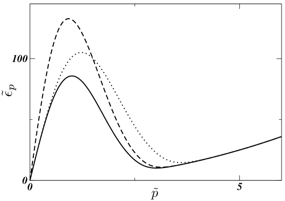
Figure 1: Excitation spectra as given by Eq. (76) for the $2$-body finite-range potential (74) (solid line), by (78) for the $3$-body finite-range potential (77) (dashed line) and by Eq. (80) for the $3$-body finite-range potential (79) (dotted line). Dimensionless units are used as explained in Section III.3: in all the three cases the dimensionless parameter, respectively $\tilde{V}$, $\tilde{{\cal V}}$ and $\tilde{{\cal V}}_{0}$, is chosen to be $10^{4}$.

IV $2$- and $3$-body $\delta$-interactions

As a first application of the results presented in Sections II and III we consider a model with $2$- and $3$-body contact interactions and we apply the obtained findings for realistic values of the trap parameters.

For a model with $2$- and $3$-body $\delta$-interactions, the Hamiltonian reads

$$\hat{H}=\int\!\mathrm{d}\mathbf{r}\,\hat{\Psi}^{\dagger}(\mathbf{r})\,\biggl{(}-\frac{\hbar^{2}\nabla^{2}}{2m}\biggr{)}\,\hat{\Psi}(\mathbf{r})+\frac{U_{2}}{2!}\int\!\mathrm{d}\mathbf{r}\,\biggl{(}\hat{\Psi}^{\dagger}(\mathbf{r})\biggr{)}^{\!2}\cdot\biggl{(}\hat{\Psi}(\mathbf{r})\biggr{)}^{\!2}+\frac{U_{3}}{3!}\int\!\mathrm{d}\mathbf{r}\,\biggl{(}\hat{\Psi}^{\dagger}(\mathbf{r})\biggr{)}^{\!3}\cdot\biggl{(}\hat{\Psi}(\mathbf{r})\biggr{)}^{\!3}\mbox{.}$$ (81)

In the Bogoliubov approximation one finds

$$\hat{H}=\biggl{(}n\frac{U_{2}}{2}+n^{2}\frac{U_{3}}{6}\biggr{)}N_{T}+\sum_{\begin{subarray}{c}\mathbf{p}\neq 0\\ (\mathbf{p}>0)\end{subarray}}\biggl{\{}\biggl{(}\epsilon_{p}^{0}+X^{(3)}\biggr{)}\biggl{(}\hat{a}_{\mathbf{p}}^{\dagger}\hat{a}_{\mathbf{p}}+\hat{a}_{-\mathbf{p}}^{\dagger}\hat{a}_{-\mathbf{p}}\biggr{)}+X^{(3)}\biggl{(}\hat{a}_{\mathbf{p}}^{\dagger}\hat{a}_{-\mathbf{p}}^{\dagger}+\hat{a}_{\mathbf{p}}\hat{a}_{-\mathbf{p}}\biggr{)}\biggr{\}}\mbox{,}$$ (82)

with

$$X^{(3)}=n_{0}U_{2}+n_{0}^{2}U_{3}\mbox{.}$$ (83)

Note that $U_{2}$ and $U_{3}$ have dimensions $[E]\!\cdot\![L]^{3}$ and $[E]\!\cdot\![L]^{6}$, respectively. The ground-state energy is found to be

$$\frac{E_{0}}{\Omega}=\biggl{(}\frac{n^{2}U_{2}}{2}+\frac{n^{3}U_{3}}{6}\biggr{)}+\frac{8}{15\pi^{2}}\biggl{(}\frac{m\,\mathfrak{s}}{\hbar}\biggr{)}^{\!3}\mbox{,}$$ (84)

with $\mathfrak{s}=\sqrt{X^{(3)}/m}=\sqrt{\bigl{(}n_{0}U_{2}+n_{0}^{2}U_{3}\bigr{)}/m}$.

The stability as a function of $U_{1}$ and $U_{2}/n_{0}$ is simply given by $X^{(3)}>0$, i.e. by

$$U_{2}+n_{0}U_{3}>0\mbox{.}$$ (85)

Using (85) we can evaluate the values of $U_{3}$ for which one has instability, as depicted in Fig. 2. To make contact with a notation often used in the literature, we set $U_{3}\equiv 2g_{3}$. Theoretical estimates for $g_{3}$ have been given in literature gammal2001 ; kohler2002 ; li2010 . Regarding one-dimensional trapping potentials, we mention that the $3$-body recombination rate in $1D$ Bose gases was experimentally studied laburthe2004 ; haller2011 , and several theoretical studies addressed the problem of determining $g_{3}$ and its effects in the Lieb-Liniger model gangardt2003 ; kheruntsyan2003 ; cheianov2006 ; kormos2009 ; kormos2011 ; piroli2015 .

Finally, the depletion fraction is given by

$$\frac{n_{ex}}{n}=\frac{\sqrt{n}}{3\pi^{2}}\biggl{(}\frac{\sqrt{m(U_{2}+nU_{3})}}{\hbar}\biggr{)}^{\!3}\mbox{,}$$ (86)

where in the right-hand side it has been used the fact that $n_{0}\approx n$.

As an application of the previous results we may consider the case of ⁸⁵Rb atoms, having a negative scattering length $a_{s}<0$ cornish2000 ; dorney2001 ; cornish2006 ; altin2010 ; mcdonald2014 ; everitt2017 . In the setup described in everitt2015 the breathing frequency of a ⁸⁵Rb gas was studied after a variation of $a_{s}$. To refer to a realistic setup and reminding that in our study we are not including $3$-body losses (so that $g_{3}=Re[g_{3}]$), we deal with an external potential having the form

$$V(\vec{r})=\frac{1}{2}m\left[\omega_{\perp}^{2}(x^{2}+y^{2})+\omega_{z}^{2}z^{2}\right]\mbox{.}$$ (87)

For an anisotropic trap of the form (87) a very simple estimate of the density $n_{0}$ can be obtained by setting $n_{0}\approx N_{T}/\Omega$ and choosing as effective volume $\Omega$ the product $\ell_{x}\ell_{y}\ell_{z}\equiv\Omega_{TF}$ of the Thomas-Fermi quantities $\ell_{\alpha}$ (with $\alpha=x,y,z$) defined in Appendix C, where we study the cubic-quintic Gross-Pitaevskii equation in an isotropic potential parabolic trap. Similarly to what is done for $2$-body interactions, to take into account in a simple way the effect of the anisotropy of the potential $V\left(\vec{r}\right)$, we use the formula (140) of Appendix C by substituting $\bar{\omega}=(\omega_{\perp}^{2}\omega_{z})^{1/3}$ in place of $\omega$ and $\bar{a}=\sqrt{\hbar/m\bar{\omega}}$ in place of $a=\sqrt{\hbar/m\omega}$ [where $\omega$ and $a$ refer to an isotropic potential $V\left(\vec{r}\right)=\frac{1}{2}m\omega^{2}\left(x^{2}+y^{2}+z^{2}\right)$, as studied in Appendix C].

In Fig.2, we report points corresponding to different values of $a_{s}<0$ cornish2000 for a set of realistic values of the parameters, together with result (85). For each value of $a_{s}$ we determine the Thomas-Fermi radius $R$ using Eq. (136) and then the quantities $\ell_{\alpha}$ via Eq. (138). An important point to be observed is that when $|a_{s}|$ increases the ratio $\ell_{\alpha}/R$ increases, but $R$ itself decreases (due to the small but appreciable attractive $2$-body interactions), finally resulting in a decrease of the effective volume and an increase of $U_{3}n_{0}$.

To illustrate the results reported in Fig.2 we introduced the dimensionless variable $u_{2}\equiv\frac{U_{2}}{\hbar\bar{\omega}\bar{a}^{3}}$ and $u_{3}\equiv\frac{U_{3}n_{0}}{\hbar\bar{\omega}\bar{a}^{3}}$, respectively proportional to $U_{2}$ and $U_{3}$. It emerges from the figure that the points lie in the stability region: similar results (even deeper in the stability region) would have been obtained if we had chosen the peak density $n(0)$ at the trap center, which is another reasonable choice. We also considered other values of $U_{3}$ to explore the dependence of the stability plot on the values of $U_{2}$, $U_{3}$, and the result is that, even with rather larger values of $U_{3}$, the system is stable. We observe that with (the very large value of) $a_{s}=-100a_{0}$, one gets $|u_{3}/u_{2}|\sim 10$. Furthermore, for a value $U_{3}$ which is, e.g., $10$ times larger than the one considered in Fig. 2, one would have again $|u_{3}/u_{2}|\sim 10$, again well inside the stability region.

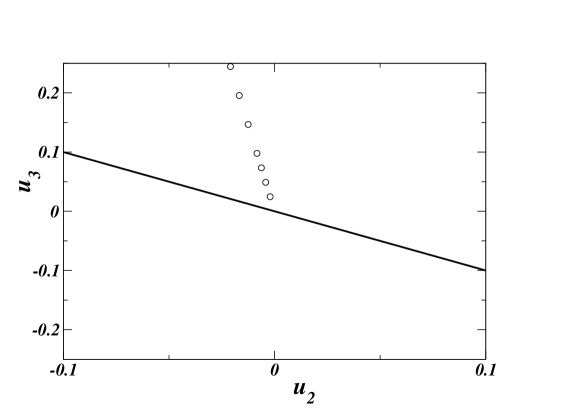
Figure 2: Plot of stability for a Bose gas with $2$- and $3$-body $\delta$-interactions according to Eq. (85). Above (below) the separation line the system is stable (unstable). We are using the notations $u_{2}\equiv U_{2}/\hbar\bar{\omega}\bar{a}^{3}$ and $u_{3}\equiv U_{3}n_{0}/\hbar\bar{\omega}\bar{a}^{3}$. The circles refer from the bottom to the values $a_{s}/a_{0}=-5,-10,-15,-20,-30,-40,-50$ with the following set of parameters: $N=10000$, $\omega_{\perp}=2\pi\cdot 100$Hz, $\omega_{z}=2\pi\cdot 10$Hz, $g_{3}=10^{-27}\hbar\cdot cm\,s^{-1}$. The density $n_{0}$ is estimated as discussed in the text and $\bar{\omega}=(\omega_{\perp}^{2}\omega_{z})^{1/3}$, $\bar{a}=\sqrt{\hbar/m\bar{\omega}}$.

V Other applications to ultracold atom systems

In this Section we discuss some further realistic interaction potentials which are of interest for current experimental setups with ultracold atoms. The discussed applications include dipolar systems, e.g. magnetic atoms and polar molecules, and soft-core potentials that can be simulated with Rydberg dressed atoms. For each of these cases we analyse the energy of the elementary excitations in the homogeneous limit and derive for some interesting parameter regimes the stability diagram of the Bogoliubov spectra.

Before discussing in detail these specific implementations let us consider a general model with a non-local $2$-body interaction potential accompanied by $2$- and $3$-body contact interactions. Note that it is possible to extend this model straightforwardly adding $\delta$-interactions up to $N$-body to a $2$-body non-local interaction potential, but for the sake of simplicity we will not consider this general case.

The Hamiltonian of the system reads

$$\begin{split}\hat{H}=\int\!\mathrm{d}\mathbf{r}\,\hat{\Psi}^{\dagger}(\mathbf{r})\,\biggl{(}\!-\frac{\hbar^{2}\nabla^{2}}{2m}\biggr{)}\,\hat{\Psi}(\mathbf{r})+&\frac{1}{2!}\int\!\mathrm{d}\mathbf{r}_{1}\mathrm{d}\mathbf{r}_{2}\,\hat{\Psi}^{\dagger}(\mathbf{r}_{1})\hat{\Psi}^{\dagger}(\mathbf{r}_{2})\,V_{2}(\mathbf{r}_{1}-\mathbf{r}_{2})\,\hat{\Psi}(\mathbf{r}_{2})\hat{\Psi}(\mathbf{r}_{1})+\\ +&\frac{U_{2}}{2!}\int\!\mathrm{d}\mathbf{r}\,\biggl{(}\hat{\Psi}^{\dagger}(\mathbf{r})\biggr{)}^{\!2}\cdot\biggl{(}\hat{\Psi}(\mathbf{r})\biggr{)}^{\!2}+\frac{U_{3}}{3!}\int\!\mathrm{d}\mathbf{r}\,\biggl{(}\hat{\Psi}^{\dagger}(\mathbf{r})\biggr{)}^{\!3}\cdot\biggl{(}\hat{\Psi}(\mathbf{r})\biggr{)}^{\!3}\mbox{.}\end{split}$$ (88)

Proceeding as in Sections II and III and expanding the quantum fields in terms of creation and annihilation operators, one arrives in the Bogoliubov approximation at the following expression for the Hamiltonian:

$$\hat{H}=\biggl{(}n\frac{V_{0}}{2}+n\frac{U_{2}}{2}+n^{2}\frac{U_{3}}{6}\biggr{)}N_{T}+\sum_{\begin{subarray}{c}\mathbf{p}\neq 0\\ (\mathbf{p}>0)\end{subarray}}\biggl{\{}\biggl{(}\epsilon_{p}^{0}+X_{\mathbf{p}}\biggr{)}\biggl{(}\hat{a}_{\mathbf{p}}^{\dagger}\hat{a}_{\mathbf{p}}+\hat{a}_{-\mathbf{p}}^{\dagger}\hat{a}_{-\mathbf{p}}\biggr{)}+X_{\mathbf{p}}\biggl{(}\hat{a}_{\mathbf{p}}^{\dagger}\hat{a}_{-\mathbf{p}}^{\dagger}+\hat{a}_{\mathbf{p}}\hat{a}_{-\mathbf{p}}\biggr{)}\biggr{\}}\mbox{,}$$ (89)

where $X_{\mathbf{p}}=n_{0}V_{\mathbf{p}}+n_{0}U_{2}+n_{0}^{2}U_{3}$ is the sum of the Fourier components of each interaction potential times the condensate density $n_{0}$ to the proper power. We then arrive at the Bogoliubov excitation spectrum:

$$\epsilon_{\mathbf{p}}=\sqrt{\bigl{(}\epsilon_{p}^{0}\bigr{)}^{2}+2\Bigl{(}n_{0}V_{\mathbf{p}}+n_{0}U_{2}+n_{0}^{2}U_{3}\Bigr{)}\,\epsilon_{p}^{0}}\mbox{.}$$ (90)

The condensate density can be obtained by solving the self-consistent equation:

$$n_{0}=n-\frac{1}{2(2\pi\hbar)^{3}}\int\!\mathrm{d}\mathbf{p}\Biggl{(}\frac{\frac{p^{2}}{2m}+n_{0}V_{\mathbf{p}}+n_{0}U_{2}+n_{0}^{2}U_{3}}{\sqrt{\bigl{(}\frac{p^{2}}{2m}\bigr{)}^{\!2}+2\bigl{(}n_{0}V_{\mathbf{p}}+n_{0}U_{2}+n_{0}^{2}U_{3}\bigr{)}\frac{p^{2}}{2m}}}-1\Biggr{)}\mbox{.}$$ (91)

An example where the stability conditions can be carried out explicitly is the Gaussian 2-body potential Eq. (74) plus a $2$- and $3$-body $\delta$-interaction. The Bogoliubov spectrum then reads

$$\tilde{\epsilon}_{p}=\sqrt{\tilde{p}^{4}+2(\tilde{V}e^{-\tilde{p}^{2}}+\tilde{U}_{2}+\tilde{U}_{3})\tilde{p}^{2}}\mbox{,}$$ (92)

with $\tilde{U}_{2}={n_{0}}\frac{U_{2}}{\varepsilon}$, $\tilde{U}_{3}={n_{0}^{2}}\frac{U_{3}}{\varepsilon}$. In Eq. (92) dimensionless units are used as in Section III.3, setting $\tilde{p}=\frac{p}{2\,\hbar\,\kappa}$, $\tilde{\epsilon}_{p}=\frac{\epsilon_{p}}{\varepsilon}$ and $\tilde{V}={\pi^{3/2}}\frac{n_{0}}{\kappa^{3}}\frac{V}{\varepsilon}$, with $\varepsilon=\frac{2\,\hbar^{2}\,\kappa^{2}}{m}$.

Setting for convenience $\tilde{U}=\tilde{U}_{2}+\tilde{U}_{3}$, we easily derive the inequality ensuring the stability for each component of the Fourier spectrum:

$$\frac{1}{2\tilde{V}}\,\tilde{p}^{2}+\frac{\tilde{U}}{\tilde{V}}>-e^{-p^{2}}\text{.}$$ (93)

We then arrive at the following conditions for the parameters $\tilde{V}$ and $\tilde{U}$:

$$\text{Stability:}\begin{cases}\tilde{V}>\dfrac{e^{-2\tilde{U}}}{2e}&\tilde{U}\leq-1/2\text{,}\vspace{3mm}\\ \tilde{V}>-\tilde{U}&\tilde{U}>-1/2\mbox{,}\end{cases}$$ (94)

which define the stability regions of the Bogoliubov spectrum.

The inequalities (94) are represented in Fig. 3. Of course, for all repulsive non-local interactions and $2$- and $3$-body contact potentials the system is stable against linear perturbations around the uniform solution. When local and non-local potentials are competing (opposite sign) or when both $\tilde{U}$ and $\tilde{V}$ are negative, it is possible to find instabilities which may signal the onset of a structured ground-state configuration. In Fig. 4 we show two cases with negative short-range interaction $\tilde{U}$ where a roton-like minimum occurs. The blue dashed line spectrum is unstable to linear perturbations for finite momentum wave-vector, signalling the onset of a modulated ground-state. This spectrum lies on the separation line of Fig. 3.

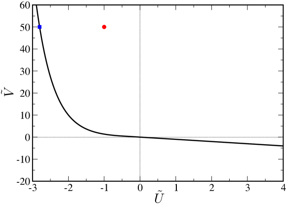
Figure 3: Stability plot for the excitation spectrum (92) as a function of the dimensionless parameters $\tilde{U}$ and $\tilde{V}$. Above (below) the separation line the uniform state is stable (unstable) against linear perturbations. Notice that competitive interactions or attractive potentials are needed to have instability. The red circle and the blue square correspond to the values of $(\tilde{U},\tilde{V})$ used in Fig. 4.

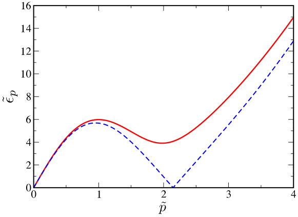
Figure 4: Excitation spectrum (92) with roton-like minima. Red line: spectrum for $\tilde{V}=50$ and $\tilde{U}=-1$ (corresponding to the red circle in Fig. 3). Blue dashed line: spectrum for $\tilde{V}=50$ and $\tilde{U}=-2.8$, where the minimum softens and the uniform solution becomes unstable signalling the onset of a new modulated ground-state. This spectrum lies on the separation line of Fig. 3 and corresponds to the blue square in Fig. 3.

V.1 $2$-body Rydberg-dressed potentials and $3$-body contact interactions

The results presented above can be applied in the case of model potentials like soft-core interactions that can be implemented in the laboratory with Rydberg-dressed potentials to see the effect of $3$-body terms. These potentials were recently created in optical lattices with Rb atoms excited to Rydberg states biedermann16 ; Zeiher16 . The interest for such interactions is general and involves the simulation of novel kinds of spin Hamiltonians vanBijnen2015 ; Glaetzle14 for the creation of exotic phases, like the supersolid boninsegni12 ; cinti14 ; leonard16 ; li16 , and for metrological applications macri16 ; davis16 ; gil14 ; henkel10 . Motivated by these experimental results and theoretical investigations, we focus on the study of the stability diagram of a $2$-body isotropic step-potential:

$$V(r)=\begin{cases}C&r\leq R_{0}\text{,}\\ 0&r>R_{0}\mbox{.}\end{cases}$$ (95)

Physically realizable potentials generically display long-range tails, decaying generically as a power law ($\sim r^{-3}$ or $\sim r^{-6}$). However, the model potential of Eq. (95) is a good approximation of such more complicated real potentials in the sense that the many-body properties found for such potential do not differ qualitatively from the realistic ones saccani12 ; kunimi12 ; macri13 ; macri14 . It is important to recall that the Gaussian model potential described above does not fall in the same class of soft-core potentials. The reason is that the Fourier transform of the Gaussian potential never changes sign, indicating that such potential alone can never display instabilities as the ones that are found for generic soft-core potentials. In the following we analyse in more detail the $3D$ as well as the $2D$ geometries in free space for the potential (95).

V.1.1 $3$D Case

In $3D$, the Fourier transform of Eq. (95) is:

$$V_{p}=a\frac{j_{1}(R_{0}p/\hbar)}{R_{0}p/\hbar}\mbox{,}$$ (96)

where $a=4\pi R_{0}^{3}C$ and $j_{1}$ is the spherical Bessel function of the 1st kind $j_{1}(x)=\frac{\sin{x}}{x^{2}}{-}\frac{\cos{x}}{x}$. From Eq. (90) the excitation spectrum is

$$\epsilon_{\mathbf{p}}=\sqrt{\bigl{(}\epsilon_{p}^{0}\bigr{)}^{2}+2\Bigl{(}4\pi\,n_{0}R_{0}^{3}\,C\,\frac{j_{1}(R_{0}p/\hbar)}{R_{0}p/\hbar}+n_{0}U_{2}+n_{0}^{2}U_{3}\Bigr{)}\,\epsilon_{p}^{0}}\mbox{.}$$ (97)

In dimensionless form this excitation spectrum can be written as

$$\tilde{\epsilon}_{p}=\sqrt{\tilde{p}^{4}+2\Bigl{(}\tilde{C}\,\frac{j_{1}(\tilde{p})}{\tilde{p}}+\tilde{U}_{2}+\tilde{U}_{3}\Bigr{)}\tilde{p}^{2}}\text{,}$$ (98)

where we defined $\tilde{p}=\frac{R_{0}p}{\hbar}$, $\varepsilon=\frac{\hbar^{4}}{2mR_{0}^{2}}$, $\tilde{\epsilon}_{p}=\frac{\epsilon_{p}}{\varepsilon}$, $\tilde{C}={4\pi n_{0}R_{0}^{3}}\frac{C}{\varepsilon}$, $\tilde{U}_{2}=\frac{n_{0}U_{2}}{\varepsilon}$ and $\tilde{U}_{3}=\frac{n_{0}^{2}U_{3}}{\varepsilon}$. Defining also $\tilde{U}=\tilde{U}_{1}+\tilde{U}_{2}$, the stability condition is represented by

$$\tilde{p}^{2}+2\tilde{C}\,\frac{j_{1}(\tilde{p})}{\tilde{p}}+2\,\tilde{U}>0\mbox{.}$$ (99)

V.1.2 $2D$ Case

The Fourier transform of Eq. (95) in $2D$ is

$$V_{p}=2\pi R_{0}^{2}C\frac{J_{1}(R_{0}p/\hbar)}{R_{0}p/\hbar}\text{,}$$ (100)

where $J_{1}(x)$ is the Bessel function of the 1st kind. The excitation spectrum is

$$\epsilon_{\mathbf{p}}=\sqrt{\bigl{(}\epsilon_{p}^{0}\bigr{)}^{2}+2\sigma_{0}\Bigl{(}2\pi R_{0}^{2}C\frac{J_{1}(R_{0}p/\hbar)}{R_{0}p/\hbar}+U_{2}+\sigma_{0}U_{3}\Bigr{)}\,\epsilon_{p}^{0}}\mbox{,}$$ (101)

with $\sigma_{0}\equiv\frac{N_{0}}{L^{2}}$. In dimensionless form this expression reads

$$\tilde{\epsilon}_{p}=\sqrt{\tilde{p}^{4}+2\Bigl{(}\tilde{C}\frac{J_{1}(\tilde{p})}{\tilde{p}}+\tilde{U}_{2}+\tilde{U}_{3}\Bigr{)}\tilde{p}^{2}}\text{,}$$ (102)

with $\tilde{C}={2\pi\sigma_{0}R_{0}^{2}}\frac{C}{\varepsilon}$, $\tilde{U}_{2}=\frac{\sigma_{0}U_{2}}{\varepsilon}$ and $\tilde{U}_{3}=\frac{\sigma_{0}^{2}U_{3}}{\varepsilon}$ with $\tilde{p}$, $\varepsilon$ and $\tilde{\epsilon}_{p}$ defined as above. Setting $\tilde{U}=\tilde{U}_{1}+\tilde{U}_{2}$, the stability condition is represented by

$$\frac{1}{2\tilde{C}}\tilde{p}^{2}+\frac{\tilde{U}}{\tilde{C}}>-\frac{J_{1}(\tilde{p})}{\tilde{p}}\mbox{.}$$ (103)

In Fig. 5 we show the stability plots for the $2D$ and $3D$ geometry in terms of the regime parameters $\tilde{C}$ and $\tilde{U}$, picking up two cases for the values $(\tilde{U},\tilde{C})$, represented by a red circle and a blue square; their respective spectra are reported in Fig. 6. Notice that, contrarily to the Gaussian potential, in $2D$ competitive interactions, or attractive potentials are not necessary to have instability.

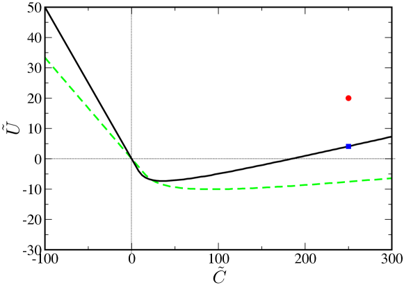
Figure 5: Stability plot for the excitation spectrum (102) as a function of the dimensionless parameters $\tilde{U}$ and $\tilde{C}$ for a $2D$ soft-core potential. Above (below) the separation line the uniform state is stable (unstable) against linear perturbations. The red circle and the blue square correspond to the values $(\tilde{U},\tilde{C})$ of the plots of Fig. 6. The green dashed line sets the stability threshold for the $3D$ soft-core potential given in Eq. (98). Above (below) the separation line the uniform state is stable (unstable) against linear perturbations.

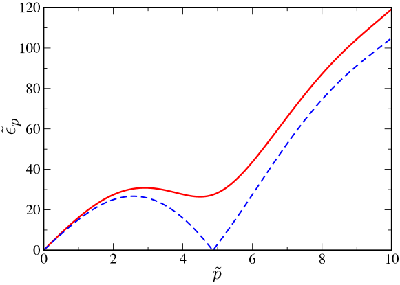
Figure 6: Excitation spectrum (102) with rotonic minima. Red line: spectrum for $\tilde{C}=250$ and $\tilde{U}=20$ (corresponding to the red circle in Fig. 5). Blue dashed line corresponding to the blue square in Fig. 5: spectrum for $\tilde{C}=250$ and $\tilde{U}=4.1$, where the minimum softens and the uniform solution becomes unstable signalling the onset of a new modulated ground-state. This spectrum lies on the separation line of Fig. 5.

V.2 Dipolar interactions in magnetic atoms and $3$-body contact interactions

In this Subsection we analyse the stability diagram of a homogeneous bosonic system interacting via a long-range $2$-body dipolar potential. Such potentials have been investigated in the past years for the study of effects induced by non-local interactions in the physics of BECs both in free space and in optical lattices lahaye09 ; baranov12 . One of the major problems regarding dipolar interaction in free space is their anisotropic character which induces instabilities in $3D$ homogeneous systems koch08 ; lahaye07 . On the other hand, the presence of an asymmetric harmonic trapping in combination with short-range repulsive interactions can eliminate such instabilities, opening the way to the study of interesting many-body physics with long-range interactions santos03 ; fischer06 . Recent experiments with dipolar BECs showed that under certain conditions where instability is expected from a standard Bogoliubov approach, dense clusters with many atoms can occur chomaz16 ; ferrier16 ; kadau16 ; schmitt16 ; ferrier16-1 , which are expected to be superfluid cinti16 . Two interpretations have been proposed to explain the stabilization of this phase, namely the presence of weak $3$-body interactions xi16 ; bisset15 and beyond mean-field effects (Lee-Huang-Yang type corrections) baillie16 ; bisset16 ; waechtler16 .

Motivated by these recent developments, we analyse in further detail the stability of uniform superfluids in the presence of long-range dipolar interactions and $2$- and $3$-body contact potentials. The dipolar potential can be written as:

$$V(\mathbf{r})=\frac{C_{dd}}{4\pi}\frac{1-3\cos^{2}{\theta}}{r^{3}}\mbox{,}$$ (104)

where $C_{dd}$ is the strength of the dipolar interaction and $\theta$ is the angle between the direction of polarization and the relative position of the particles. Tuning the relative angle among the particles and the quantization axis the potential can be either attractive and repulsive. The Fourier transform of Eq. (104) is

$$V_{\mathbf{p}}=C_{dd}\Bigl{(}\cos^{2}{\alpha}-\frac{1}{3}\Bigr{)}\mbox{,}$$ (105)

where $\alpha$ is the angle between $\mathbf{p}$ and the polarization direction (of the dipole-dipole interaction).

The excitation spectrum is then found to be:

$$\epsilon_{\mathbf{p}}=\sqrt{\bigl{(}\epsilon_{p}^{0}\bigr{)}^{2}\!+2\Bigl{[}n_{0}\,C_{dd}\Bigl{(}\cos^{2}{\alpha}-\frac{1}{3}\Bigr{)}\!+n_{0}U_{2}+n_{0}^{2}\,U_{3}\Bigr{]}\,\epsilon_{p}^{0}}\mbox{,}$$ (106)

with condensate density given by the equation

$$n_{0}=n-\frac{1}{2(2\pi\hbar)^{3}}\int\!\mathrm{d}\mathbf{p}\Biggl{(}\frac{\frac{p^{2}}{2m}+n_{0}\,C_{dd}(\cos^{2}{\alpha}-\frac{1}{3})\!+n_{0}U_{2}+n_{0}^{2}\,U_{3}}{\sqrt{\bigl{(}\frac{p^{2}}{2m}\bigr{)}^{\!2}+2\bigl{[}n_{0}\,C_{dd}(\cos^{2}{\alpha}-\frac{1}{3})\!+n_{0}U_{2}+n_{0}^{2}\,U_{3}\bigr{]}\frac{p^{2}}{2m}}}-1\Biggr{)}\mbox{.}$$ (107)

The spectrum (106) can be expressed in terms of the ratio

$$\varepsilon_{dd}=\frac{a_{dd}}{a_{s}}=\frac{C_{dd}}{3U_{2}}$$ (108)

of the dipolar length $a_{dd}=\frac{C_{dd}\,m}{12\pi\hbar^{2}}$ to the $s$-wave scattering length, which compares the relative strength of the dipolar and contact interactions:

$$\epsilon_{\mathbf{p}}=\sqrt{\bigl{(}\epsilon_{p}^{0}\bigr{)}^{2}\!+2\,n_{0}\Bigl{[}3\,\varepsilon_{dd}\,U_{2}\Bigl{(}\cos^{2}{\alpha}-\frac{1}{3}\Bigr{)}\!+U_{2}+n_{0}\,U_{3}\Bigr{]}\,\epsilon_{p}^{0}}\mbox{.}$$ (109)

In dimensionless units one gets

$$\tilde{\epsilon}_{p}=\sqrt{\tilde{p}^{4}+2\Bigl{[}\Bigl{(}3\,\varepsilon_{dd}\cos^{2}{\alpha}-\varepsilon_{dd}+1\Bigr{)}\tilde{U}_{2}+\tilde{U}_{3}\Bigr{]}\tilde{p}^{2}}\text{,}$$ (110)

where $\tilde{p}=\frac{p\,a_{dd}}{\hbar}$, $\tilde{\epsilon}_{p}=\frac{\epsilon_{p}}{\varepsilon}$, $\tilde{U}_{2}=\frac{n_{0}U_{2}}{\varepsilon}$ and $\tilde{U}_{3}=\frac{n_{0}^{2}U_{3}}{\varepsilon}$, with $\varepsilon=\frac{\hbar^{2}}{2ma_{dd}^{2}}$.

In Fig. 7 we plot the stability diagram of Eq. (110) as a function of the dimensionless parameters $\tilde{U}=\tilde{U}_{2}+\tilde{U}_{3}$ and $\tilde{C}=\varepsilon_{dd}\tilde{U}_{2}$ for $\alpha=\pi/2$. We compute the specific values of these parameters for a condensate of ¹⁶⁴Dy also considering as the $3$-body contact interaction the value given in bisset15 (notice however that by using other values of $U_{3}$, as the ones given in waechtler16 , the effect of such terms is anyway rather small). From Fig. 7 one sees that upon varying the scattering length the uniform phase goes from a stable (blue diamond) to an unstable (red circle) configuration. Note that the $3$-body interaction enhances the stability region to values of $\varepsilon_{dd}$ larger than $1$.

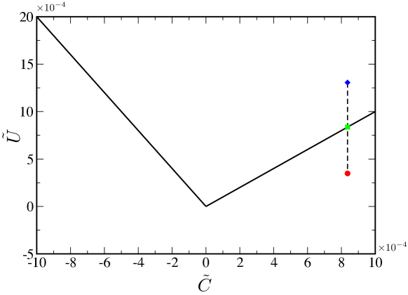
Figure 7: Stability plot for the excitation spectrum (110) as a function of the dimensionless parameters $\tilde{U}=\tilde{U}_{2}+\tilde{U}_{3}$ and $\tilde{C}=\varepsilon_{dd}\tilde{U}_{2}$ for $\alpha=\pi/2$ for a $3D$ dipolar potential and contact potentials. Above (below) the separation line the uniform state is stable (unstable) against linear perturbations. Data points correspond to three different values of the scattering length for ¹⁶⁴Dy atoms: $a_{s}=50\,a_{0}$ (red circle), $a_{s}=126\,a_{0}$ (green square), and $a_{s}=200\,a_{0}$ (blue diamond), where $a_{0}$ is the Bohr radius. In the calculations we included a $3$-body contact interaction potential using the value $U_{3}=5.87\cdot 10^{-27}\,\hbar\,cm^{6}\,s^{-1}$ considered in bisset15 , which slightly enhances the stability region of the uniform phase to $\varepsilon_{dd}<1.05$ (green square). More quantitatively, putting $U_{3}=0$ one would have the green square on the stability line for $a_{s}=a_{dd}=131\,a_{0}$. Here we set the average density $n_{0}=2\cdot 10^{20}\,m^{-3}$ and the dipolar length $a_{dd}=131\,a_{0}$.

VI Conclusions

In this work we have presented a systematic study of weakly interacting bosonic gases with local and non-local multi-body interactions in the Bogoliubov approximation. We considered conservative multi-body interactions for which the number of particles is conserved. In fact multi-body interactions are associated with the presence of particle losses kagan1985 , that we did not study, rather focusing on the determination of the stability conditions due to the competition between $2$- and higher-body interactions.

A variety of interparticle potentials have been considered. We first considered contact interactions, studying the case in which the interparticle potential can be written as a general sum of $N$-body $\delta$-interactions, providing the quasi-particle spectrum, the ground-state energy and the stability conditions. Results for general effective contact potentials are also presented. Our findings show that the well-known results for the $2$-body $\delta$-interactions in the homogeneous case are generalized in the Bogoliubov approximation by the substitution $U_{2}n_{0}\to X$, where $X$ is a function of the condensate fraction $n_{0}$ given by Eq. (24) for potentials which are sums of $N$-body $\delta$-potentials and by Eq. (45) in the general case. Since the Bogoliubov approximation works well when $n_{0}\approx n$, then one can make the substitution $n_{0}\to n$ in $X$, resulting for a sum of $N$-body contact interactions in the substitution $U_{2}n\to\sum_{\ell}U_{\ell}\ell(\ell-1)n^{\ell-1}/\ell!$. The case of higher-body non-local interactions is instead different from this respect and the final results depend on the specific form of the interactions. We explicitly considered two different cases of $3$-body non-local interactions.

In the last part we discussed a few interaction potentials which are of interest for current experimental setups with ultracold atoms. Implementations include systems with $2$- and $3$-body $\delta$-interactions, where we applied in the homogeneous limit for realistic values of the trap parameters. We also considered the effect of (conservative) $3$-body terms in dipolar systems, e.g. magnetic atoms and polar molecules, and soft-core potentials that can be simulated with Rydberg dressed atoms. For each of these cases we analysed the energy of the elementary excitations and derived the stability diagram of the Bogoliubov spectra for some interesting parameter regimes.

In the present paper we focused on higher-body interactions in the homogeneous limit, having in mind both $3$-body terms and general effective multi-body interactions. Of course ultracold experiments are done in confined traps, and we think that a systematic study of the Bogoliubov equations in inhomogeneous potentials with general multi-body local and non-local interactions is an interesting direction of future research.

Appendix A Bogoliubov approximation for a general contact interaction

In this Appendix we consider the case of a general contact interaction described by a Hamiltonian of the form

$$\hat{H}=\hat{H}_{0}+\hat{H}_{I}=\int\!\mathrm{d}\mathbf{r}\,\hat{\Psi}^{\dagger}(\mathbf{r})\,\biggl{(}-\frac{\hbar^{2}\nabla^{2}}{2m}\biggr{)}\,\hat{\Psi}(\mathbf{r})+\int\!\mathrm{d}\mathbf{r}\,\colon\!{\cal F}\!\left(\hat{\rho}\right)\!\colon\mbox{.}$$ (111)

One has

$$\hat{H}_{I}=\int\!\mathrm{d}\mathbf{r}\,\colon\!{\cal F}\!\left(\hat{\rho}\right)\!\colon =\int\!\mathrm{d}\mathbf{r}\,\colon\!{\cal F}\Biggl{(}\frac{1}{\Omega}\sum_{\mathbf{p},\mathbf{p^{\prime}}}e^{-\frac{i}{\hbar}(\mathbf{p}^{\prime}\!-\mathbf{p})\cdot\mathbf{r}}\,\hat{a}_{\mathbf{p^{\prime}}}^{\dagger}\hat{a}_{\mathbf{p}}\Biggr{)}\!\colon$$ (112)

$$=\int\!\mathrm{d}\mathbf{r}\,\colon\!{\cal F}\Biggl{(}\frac{N_{0}}{\Omega}+\frac{\sqrt{N_{0}}}{\Omega}\sum_{\mathbf{p}\neq 0}\biggl{(}e^{-\frac{i}{\hbar}\mathbf{p}\cdot\mathbf{r}}\,\hat{a}_{\mathbf{p}}^{\dagger}+e^{\frac{i}{\hbar}\mathbf{p}\cdot\mathbf{r}}\,\hat{a}_{\mathbf{p}}\biggr{)}+\frac{1}{\Omega}\sum_{\mathbf{p},\mathbf{p^{\prime}}\neq 0}e^{-\frac{i}{\hbar}(\mathbf{p}^{\prime}\!-\mathbf{p})\cdot\mathbf{r}}\,\hat{a}_{\mathbf{p^{\prime}}}^{\dagger}\hat{a}_{\mathbf{p}}\Biggr{)}\!\colon\text{,}$$

where we wrote explicitly the operator $\hat{\rho}$ in terms of the operators $\{\hat{a}_{\mathbf{p}}$, $\hat{a}_{\mathbf{p}}^{\dagger}\}$ and we used the Bogoliubov approximation. We assume that the function ${\cal F}={\cal F}(x)$ can be expanded in series up to the second order.

Since $N_{0}\approx N_{T}$ and $N_{T}\gg 1$, it follows that ${N_{0}}\gg\sqrt{N_{0}}\gg 1$, we can write:

$${\cal F}\!\left(\hat{\rho}\right)\simeq{\cal F}(n_{0})+\frac{\partial{\cal F}\!\left(x\right)}{\partial x}\bigg{|}_{x=n_{0}}\!\!\!\!\!\!\!\!\cdot\,\,\Gamma+\frac{1}{2!}\frac{\partial^{2}{\cal F}\!\left(x\right)}{\partial x^{2}}\bigg{|}_{x=n_{0}}\!\!\!\!\!\!\!\!\cdot\,\,\Gamma^{2}\,+\cdots\mbox{,}$$ (113)

where

$$\Gamma=\sqrt{\frac{n_{0}}{\Omega}}\sum_{\mathbf{p}\neq 0}\biggl{(}e^{-\frac{i}{\hbar}\mathbf{p}\cdot\mathbf{r}}\,\hat{a}_{\mathbf{p}}^{\dagger}+e^{\frac{i}{\hbar}\mathbf{p}\cdot\mathbf{r}}\,\hat{a}_{\mathbf{p}}\biggr{)}+\frac{1}{\Omega}\sum_{\mathbf{p},\mathbf{p^{\prime}}\neq 0}e^{-\frac{i}{\hbar}(\mathbf{p}^{\prime}\!-\mathbf{p})\cdot\mathbf{r}}\,\hat{a}_{\mathbf{p^{\prime}}}^{\dagger}\hat{a}_{\mathbf{p}}\mbox{.}$$ (114)

Neglecting products of 3 or more operators, the interaction part reads

$$\hat{H}_{I} =\int\!\mathrm{d}\mathbf{r}\,\colon\!\!\begin{aligned} \biggl{\{}&{\cal F}(n_{0})+\frac{\partial{\cal F}\!\left(x\right)}{\partial x}\bigg{|}_{x=n_{0}}\!\biggl{(}\!\sqrt{\frac{n_{0}}{\Omega}}\sum_{\mathbf{p}\neq 0}\Bigl{(}e^{-\frac{i}{\hbar}\mathbf{p}\cdot\mathbf{r}}\,\hat{a}_{\mathbf{p}}^{\dagger}+e^{\frac{i}{\hbar}\mathbf{p}\cdot\mathbf{r}}\,\hat{a}_{\mathbf{p}}\Bigr{)}+\frac{1}{\Omega}\sum_{\mathbf{p},\mathbf{p^{\prime}}\neq 0}e^{-\frac{i}{\hbar}(\mathbf{p}^{\prime}\!-\mathbf{p})\cdot\mathbf{r}}\,\hat{a}_{\mathbf{p^{\prime}}}^{\dagger}\hat{a}_{\mathbf{p}}\biggr{)}+\\ &+\frac{1}{2!}\frac{\partial^{2}{\cal F}\!\left(x\right)}{\partial x^{2}}\bigg{|}_{x=n_{0}}\!\biggl{(}\frac{n_{0}}{\Omega}\!\sum_{\mathbf{p},\mathbf{p^{\prime}}\neq 0}\Bigl{(}e^{-\frac{i}{\hbar}\mathbf{p}\cdot\mathbf{r}}\,\hat{a}_{\mathbf{p}}^{\dagger}+e^{\frac{i}{\hbar}\mathbf{p}\cdot\mathbf{r}}\,\hat{a}_{\mathbf{p}}\Bigr{)}\Bigl{(}e^{-\frac{i}{\hbar}\mathbf{p}^{\prime}\!\cdot\mathbf{r}}\,\hat{a}_{\mathbf{p}^{\prime}}^{\dagger}+e^{\frac{i}{\hbar}\mathbf{p}^{\prime}\!\cdot\mathbf{r}}\,\hat{a}_{\mathbf{p}^{\prime}}\Bigr{)}\!\biggr{)}\!\biggr{\}}\colon\end{aligned}$$ (115)

$$={\cal F}(n_{0})\,\Omega\begin{aligned} &+\frac{\partial{\cal F}\!\left(x\right)}{\partial x}\bigg{|}_{x=n_{0}}\sum_{\mathbf{p}\neq 0}\hat{a}_{\mathbf{p}}^{\dagger}\hat{a}_{\mathbf{p}}+\\ &+\frac{1}{2!}n_{0}\frac{\partial^{2}{\cal F}\!\left(x\right)}{\partial x^{2}}\bigg{|}_{x=n_{0}}\sum_{\mathbf{p}\neq 0}\Bigl{(}2\hat{a}_{\mathbf{p}}^{\dagger}\hat{a}_{\mathbf{p}}+\hat{a}_{\mathbf{p}}^{\dagger}\hat{a}_{-\mathbf{p}}^{\dagger}+\hat{a}_{\mathbf{p}}\hat{a}_{-\mathbf{p}}\Bigr{)}\text{,}\end{aligned}$$

where we integrated out the space variable and used the conservation of momentum, having taken explicitly the normal ordering of the operators. Using the conservation of the total number of particles, we can write

$${\cal F}(n_{0})\simeq{\cal F}(n)-\frac{\partial{\cal F}\!\left(x\right)}{\partial x}\bigg{|}_{x=n}\frac{1}{\Omega}\sum_{\mathbf{p}\neq 0}\hat{a}_{\mathbf{p}}^{\dagger}\hat{a}_{\mathbf{p}}\text{,}$$ (116)

so that

$$\hat{H}_{I} ={\cal F}(n)\,\Omega\begin{aligned} &+\biggl{(}\frac{\partial{\cal F}\!\left(x\right)}{\partial x}\bigg{|}_{x=n_{0}}\!\!\!\!\!\!\!-\,\,\,\frac{\partial{\cal F}\!\left(x\right)}{\partial x}\bigg{|}_{x=n}\biggr{)}\!\sum_{\mathbf{p}\neq 0}\hat{a}_{\mathbf{p}}^{\dagger}\hat{a}_{\mathbf{p}}+\\ &+\frac{1}{2!}n_{0}\frac{\partial^{2}{\cal F}\!\left(x\right)}{\partial x^{2}}\bigg{|}_{x=n_{0}}\sum_{\mathbf{p}\neq 0}\Bigl{(}2\hat{a}_{\mathbf{p}}^{\dagger}\hat{a}_{\mathbf{p}}+\hat{a}_{\mathbf{p}}^{\dagger}\hat{a}_{-\mathbf{p}}^{\dagger}+\hat{a}_{\mathbf{p}}\hat{a}_{-\mathbf{p}}\Bigr{)}\text{.}\end{aligned}$$ (117)

Denoting ${\cal G}(y)\equiv\frac{\partial{\cal F}\left(x\right)}{\partial x}\Big{|}_{x=y}$, we see that

$${\cal G}(n_{0})-{\cal G}(n)\simeq-\frac{\partial{\cal G}(x)}{\partial x}\bigg{|}_{x=n}\frac{1}{\Omega}\sum_{\mathbf{p}\neq 0}\hat{a}_{\mathbf{p}}^{\dagger}\hat{a}_{\mathbf{p}}\text{,}$$ (118)

so that the difference in the second term of the previous equation is of higher order and it can be safely neglected. Thus the complete Hamiltonian can be written as

$$\hat{H}={\cal F}(n)\,\Omega+\!\sum_{\begin{subarray}{c}\mathbf{p}\neq 0\\ (\mathbf{p}>0)\end{subarray}}\!\biggl{\{}\!\biggl{(}\!\epsilon_{p}^{0}\!+\!n_{0}\frac{\partial^{2}{\cal F}\!\left(x\right)}{\partial x^{2}}\bigg{|}_{x=n_{0}}\biggr{)}\!\Bigl{(}\hat{a}_{\mathbf{p}}^{\dagger}\hat{a}_{\mathbf{p}}+\hat{a}_{-\mathbf{p}}^{\dagger}\hat{a}_{-\mathbf{p}}\Bigr{)}+n_{0}\frac{\partial^{2}{\cal F}\!\left(x\right)}{\partial x^{2}}\bigg{|}_{x=n_{0}}\!\!\Bigl{(}\hat{a}_{\mathbf{p}}^{\dagger}\hat{a}_{-\mathbf{p}}^{\dagger}+\hat{a}_{\mathbf{p}}\hat{a}_{-\mathbf{p}}\Bigr{)}\!\biggr{\}}\mbox{,}$$ (119)

from which Eq. (44) follows.

Appendix B Excitation spectrum for a $3$-body non-local factorizable potential

In this Appendix we consider the $3$-body finite-range potential of Eq. (61):

$$U(\mathbf{r}_{1},\mathbf{r}_{2},\mathbf{r}_{3})=V(\mathbf{r}_{1}-\mathbf{r}_{2})V(\mathbf{r}_{2}-\mathbf{r}_{3})V(\mathbf{r}_{3}-\mathbf{r}_{1})\mbox{,}$$ (120)

where $V(\mathbf{r})=V(r)$. In momentum space, the Hamiltonian can be written as $\hat{H}=\hat{H_{0}}+\hat{H}_{I}$ with the kinetic term $\hat{H_{0}}$ given by Eq. (7). To write the interaction term $\hat{H}_{I}$, we consider here the change of variables {$\mathbf{r}_{1},\mathbf{r}_{2},\mathbf{r}_{3}$} $\rightarrow$ {$\mathbf{r}_{12},\mathbf{r}_{31},\mathbf{R}$}, where

$$\begin{split}&\mathbf{r}_{12}=\mathbf{r}_{1}-\mathbf{r}_{2}\mbox{,}\\ &\mathbf{r}_{31}=\mathbf{r}_{3}-\mathbf{r}_{1}\mbox{,}\\ &\mathbf{R}=\frac{\mathbf{r}_{1}+\mathbf{r}_{2}+\mathbf{r}_{3}}{3}\mbox{.}\end{split}$$ (121)

In the Bogoliubov approximation, after some algebra we obtain

$$\hat{H}_{I}= \frac{N_{0}^{3}}{6\Omega^{2}}\!\int\!\mathrm{d}\mathbf{r}_{12}\,\mathrm{d}\mathbf{r}_{31}\,V(r_{12})V(r_{31})V(r_{12}\!+\!r_{31})+$$ (122)

$$+\frac{N_{0}^{2}}{6\Omega^{2}}\sum_{\mathbf{p}\neq 0}\begin{aligned} \biggl{\{}&\int\!\mathrm{d}\mathbf{r}_{12}\,\mathrm{d}\mathbf{r}_{31}\,\mathfrak{F}_{\mathbf{p}}(\mathbf{r}_{12},\mathbf{r}_{31})V(r_{12})V(r_{31})V(r_{12}\!+\!r_{31})\Bigl{(}\hat{a}_{\mathbf{p}}^{\dagger}\hat{a}_{-\mathbf{p}}^{\dagger}\!+\!\hat{a}_{\mathbf{p}}\hat{a}_{-\mathbf{p}}\Bigr{)}\!+\\ &\!+\!\!\int\!\mathrm{d}\mathbf{r}_{12}\,\mathrm{d}\mathbf{r}_{31}\Bigl{[}3+2\,\mathfrak{F}_{\mathbf{p}}(\mathbf{r}_{12},\mathbf{r}_{31})\Bigr{]}V(r_{12})V(r_{31})V(r_{12}\!+\!r_{31})\hat{a}_{\mathbf{p}}^{\dagger}\hat{a}_{\mathbf{p}}\biggr{\}}\mbox{,}\end{aligned}$$

where we defined

$$\mathfrak{F}_{\mathbf{p}}(\mathbf{r}_{12},\mathbf{r}_{31})=\Bigl{(}e^{-\frac{i}{\hbar}\mathbf{p}\cdot\mathbf{r}_{12}}+e^{-\frac{i}{\hbar}\mathbf{p}\cdot\mathbf{r}_{31}}+e^{-\frac{i}{\hbar}\mathbf{p}\cdot(\mathbf{r}_{12}+\mathbf{r}_{31})}\Bigr{)}\mbox{.}$$ (123)

Setting

$$C=\int\!\mathrm{d}\mathbf{r}_{12}\,\mathrm{d}\mathbf{r}_{31}\,V(r_{12})V(r_{13})V(r_{12}+r_{13})\mbox{,}$$ (124)

proceeding as in Section III.1, one can write the Hamiltonian in the form

$$\hat{H}=\frac{N_{T}^{3}}{6\Omega^{2}}C\!+\!\!\sum_{\mathbf{p}>0}\begin{aligned} \biggl{\{}&\biggl{[}\epsilon_{p}^{0}\!+\!\frac{n_{0}^{2}}{3}\!\!\int\!\!\mathrm{d}\mathbf{r}_{12}\,\mathrm{d}\mathbf{r}_{31}\,\mathfrak{F}_{\mathbf{p}}(\mathbf{r}_{12},\mathbf{r}_{31})V(r_{12})V(r_{31})V(r_{12}\!+\!r_{31})\biggr{]}\Bigl{(}\hat{a}_{\mathbf{p}}^{\dagger}\hat{a}_{\mathbf{p}}\!+\!\hat{a}_{-\mathbf{p}}^{\dagger}\hat{a}_{-\mathbf{p}}\Bigr{)}+\\ &+\frac{n_{0}^{2}}{3}\!\int\!\!\mathrm{d}\mathbf{r}_{12}\,\mathrm{d}\mathbf{r}_{31}\,\mathfrak{F}_{\mathbf{p}}(\mathbf{r}_{12},\mathbf{r}_{31})V(r_{12})V(r_{31})V(r_{12}\!+\!r_{31})\Bigl{(}\hat{a}_{\mathbf{p}}^{\dagger}\hat{a}_{-\mathbf{p}}^{\dagger}\!+\!\hat{a}_{\mathbf{p}}\hat{a}_{-\mathbf{p}}\Bigr{)}\biggr{\}}\mbox{,}\end{aligned}$$ (125)

which is diagonalizable by the standard procedure. Then the excitation spectrum is:

$$\epsilon_{p}=\sqrt{\bigl{(}\epsilon_{p}^{0}\bigr{)}^{2}+\frac{2}{3}n_{0}^{2}\Bigl{(}\int\!\mathrm{d}\mathbf{r}_{12}\,\mathrm{d}\mathbf{r}_{31}\,\mathfrak{F}_{\mathbf{p}}(\mathbf{r}_{12},\mathbf{r}_{31})V(r_{12})V(r_{31})V(r_{12}+r_{31})\Bigr{)}\,\epsilon_{p}^{0}\biggr{]}},$$ (126)

and we obtain

$$\epsilon_{p}=\sqrt{\bigl{(}\epsilon_{p}^{0}\bigr{)}^{2}+\frac{2}{3}n_{0}^{2}\Bigl{(}\int\!\mathrm{d}\mathbf{r}_{12}\,\mathrm{d}\mathbf{r}_{31}\Bigl{(}e^{-\frac{i}{\hbar}\mathbf{p}\cdot\mathbf{r}_{12}}+e^{-\frac{i}{\hbar}\mathbf{p}\cdot\mathbf{r}_{31}}+e^{-\frac{i}{\hbar}\mathbf{p}\cdot(\mathbf{r}_{12}+\mathbf{r}_{31})}\Bigr{)}V(r_{12})V(r_{31})V(r_{12}+r_{31})\Bigr{)}\,\epsilon_{p}^{0}\biggr{]}\mbox{.}}$$ (127)

To demonstrate the equivalence between Eqs. (127) and (71) we have to show that their prefactors multiplying $\epsilon_{p}^{0}$ are equal. We start considering the factor of Eq. (127), which we denote by $f_{\mathbf{p}}$:

$$f_{\mathbf{p}}\equiv\frac{2}{3}n_{0}^{2}\!\int\!\mathrm{d}\mathbf{r}_{12}\,\mathrm{d}\mathbf{r}_{31}\Bigl{(}e^{-\frac{i}{\hbar}\mathbf{p}\cdot\mathbf{r}_{12}}+e^{-\frac{i}{\hbar}\mathbf{p}\cdot\mathbf{r}_{31}}+e^{-\frac{i}{\hbar}\mathbf{p}\cdot(\mathbf{r}_{12}+\mathbf{r}_{31})}\Bigr{)}V(r_{12})V(r_{31})V(r_{12}+r_{31})\mbox{.}$$ (128)

Since

$$V(r_{12})V(r_{31})V(r_{12}\!+\!r_{31})=\frac{1}{\Omega^{3}}\!\!\sum_{\begin{subarray}{c}\mathbf{p}_{12}\\ \mathbf{p}_{31}\\ \mathbf{p}_{12+31}\end{subarray}}\!\!V_{\mathbf{p}_{12}}\,V_{\mathbf{p}_{31}}\,V_{\mathbf{p}_{12+31}}\,e^{\frac{i}{\hbar}\mathbf{p}_{12}\cdot\mathbf{r}_{12}}\,e^{\frac{i}{\hbar}\mathbf{p}_{31}\cdot\mathbf{r}_{31}}e^{\frac{i}{\hbar}\mathbf{p}_{12+31}\cdot(\mathbf{r}_{12}+\mathbf{r}_{31})}\mbox{,}$$ (129)

inserting this expression in (128), it is readily seen that $f_{\mathbf{p}}$ is given by

$$f_{\mathbf{p}}=\frac{2}{3}\frac{n_{0}^{2}}{\Omega}\!\!\sum_{\begin{subarray}{c}\mathbf{p}_{12}\\ \mathbf{p}_{31}\\ \mathbf{p}_{12+31}\end{subarray}}\!\!V_{\mathbf{p}_{12}}\,V_{\mathbf{p}_{31}}\,V_{\mathbf{p}_{12+31}}\biggl{\{}\delta_{\mathbf{p},\mathbf{p}_{12}+\mathbf{p}_{12+31}}\delta_{\mathbf{p}_{31},-\mathbf{p}_{12+31}}+\delta_{\mathbf{p}_{12},-\mathbf{p}_{12+31}}\delta_{\mathbf{p},\mathbf{p}_{31}+\mathbf{p}_{12+31}}+\delta_{\mathbf{p},\mathbf{p}_{12}+\mathbf{p}_{12+31}}\delta_{\mathbf{p},\mathbf{p}_{31}+\mathbf{p}_{12+31}}\biggr{\}}\mbox{,}$$ (130)

which is equal to

$$f_{\mathbf{p}}=\frac{2}{3}\frac{n_{0}^{2}}{\Omega}\sum_{\mathbf{p}_{12}}\biggl{\{}V_{\mathbf{p}_{12}}\,V_{\mathbf{p}_{12}-\mathbf{p}}\,V_{-\mathbf{p}_{12}+\mathbf{p}}+V_{\mathbf{p}_{12}}\,V_{\mathbf{p}+\mathbf{p}_{12}}\,V_{-\mathbf{p}_{12}}+V_{\mathbf{p}_{12}}^{2}\,V_{-\mathbf{p}_{12}+\mathbf{p}}\biggr{\}}\mbox{.}$$ (131)

Using in the previous expression the properties $\sum_{\mathbf{p}}V_{\mathbf{p}}=\sum_{\mathbf{p}}V_{-\mathbf{p}}$ and

$$\sum_{\mathbf{p}_{12}}V_{\mathbf{p}_{12}}^{2}\,V_{\mathbf{p}_{12}+\mathbf{p}}=\sum_{\mathbf{p}_{12}}V_{\mathbf{p}_{12}}^{2}\,V_{-\mathbf{p}_{12}+\mathbf{p}}\mbox{,}$$ (132)

we retrieve the prefactor of the $\epsilon_{p}^{0}$ term in Eq. (71).

Appendix C Thomas-Fermi approximation for the cubic-quintic Gross-Pitaevskii in an isotropic parabolic trap

In this Appendix we consider the time-independent cubic-quintic Gross-Pitaevskii equation

$$-\frac{\hbar^{2}}{2m}\nabla^{2}\psi+V\psi+g_{2}|\psi|^{2}\psi+g_{3}|\psi|^{4}\psi=\mu\psi\mbox{,}$$ (133)

where the parabolic trap $V(\mathbf{r})$ is assumed isotropic:

$$V(\mathbf{r})=\frac{1}{2}m\omega^{2}(x^{2}+y^{2}+z^{2})\mbox{.}$$ (134)

To make contact with the notation used in the main text, it is $U_{2}=g_{2}$ and $g_{3}=U_{3}/2$.

In the Thomas-Fermi approximation pethick2002 ; pitaevskii2016 it is found with $g_{3}>0$ that

$$|\psi(\vec{r})|^{2}=\frac{\sqrt{g_{2}^{2}+4g_{3}[\mu-V(\vec{r})]}-g_{2}}{2g_{3}}\mbox{.}$$ (135)

Imposing the normalization condition $\int d\vec{r}\,|\psi|^{2}=N$ and defining the Thomas-Fermi radius $R$ such that $V(R)=\mu$, one gets

$$N=A{\cal R}^{4}F\left(\frac{B}{{\cal R}^{2}}\right)-C{\cal R}^{3}\mbox{,}$$ (136)

where ${\cal R}$ is measured in units of the harmonic oscillator length $a=\sqrt{\hbar/m\omega}$ (with ${\cal R}\equiv R/a$) and the dimensionless quantities $A$, $B$ and $C$ in Eq. (136) are given by $A={2\pi}\sqrt{\frac{2m\omega^{2}}{g_{3}}}{a^{4}}$, $B=\frac{g_{2}^{2}}{2g_{3}\hbar\omega}$ and $C=\frac{2\pi g_{2}a^{3}}{3g_{3}}$. In (136) the function $F(x)$ is defined (with $x>0$) as

$$F(x)=\int_{0}^{1}\theta^{2}\sqrt{1+x-\theta^{2}}d\theta=\frac{1}{8}\left[\left(1-x\right)\sqrt{x}+\left(1+x\right)^{2}\mathrm{arccsc}\left(\sqrt{1+x}\right)\right]\mbox{.}$$ (137)

The expectation value of $\langle r^{2}\rangle=\frac{\int d\vec{r}r^{2}|\psi|^{2}}{N}$ is given by

$$\frac{\langle r^{2}\rangle}{R^{2}}=\frac{A{\cal R}^{4}G\left(\frac{B}{{\cal R}^{2}}\right)-\frac{3}{5}C{\cal R}^{3}}{N}\mbox{,}$$ (138)

where $R$ is defined by Eq. (136) and the function $G$ is given by

$$G(x)=\int_{0}^{1}\theta^{4}\sqrt{1+x-\theta^{2}}d\theta=\frac{1}{48}\left[\left(1-3x\right)\left(3+x\right)\sqrt{x}+3\left(1+x\right)^{3}\mathrm{arccsc}\left(\sqrt{1+x}\right)\right]\mbox{.}$$ (139)

Since $\langle r^{2}\rangle=\langle x^{2}\rangle+\langle y^{2}\rangle+\langle z^{2}\rangle$, we get $\langle x^{2}\rangle=\langle y^{2}\rangle=\langle z^{2}\rangle=\langle r^{2}\rangle/3$. To adapt the notation to that of the main text, we set $\sigma_{\alpha}\equiv\sqrt{\langle\alpha^{2}\rangle}$ and $\ell_{\alpha}\equiv 2\sigma_{\alpha}$, with $\alpha=x,y,z$, so that in the isotropic case considered in this Appendix the product $\ell_{x}\ell_{y}\ell_{z}$, which we denote by $\Omega_{TF}$, reads

$$\Omega_{TF}=\frac{8}{3\sqrt{3}}\,\langle r^{2}\rangle^{3/2}\mbox{,}$$ (140)

where $\langle r^{2}\rangle$ is given by Eq. (138).

The previous formulas simplify for $g_{2}=0$, when only the $3$-body interaction term [i.e., only the quintic term in the Gross-Pitaevskii equation (133)] is present. One gets

$$\frac{R^{4}}{a^{4}}=\frac{4N\sqrt{2{\cal G}_{3}}}{\pi^{2}}\mbox{,}$$ (141)

where we introduced the dimensionless parameter ${\cal G}_{3}\equiv\frac{g_{3}}{\hbar\omega a^{6}}$ (remember that $[g_{3}]=[E]\,\cdot\,[L]^{6}$). The expectation value of $\langle r^{2}\rangle$ is simply given by

$$\langle r^{2}\rangle=\frac{R^{2}}{2}\mbox{.}$$ (142)

Eqs. (141) and (142) have to be compared with the usual results for the cubic Gross-Pitaevskii (with $g_{3}=0$), where one has respectively

$$\frac{R^{5}}{a^{5}}=\frac{15N{\cal G}_{2}}{4\pi}\mbox{,}$$ (143)

(where ${\cal G}_{2}\equiv\frac{g_{2}}{\hbar\omega a^{3}}$) and

$$\langle r^{2}\rangle=\frac{3R^{2}}{7}\mbox{.}$$ (144)

References

• (1) N. N. Bogoliubov, J. Phys. (USSR) 11, 23 (1947).
• (2) V. A. Zagrebnov and J.-B. Bru, Phys. Rep. 350, 291 (2001).
• (3) C. Pethick and H. Smith, Bose-Einstein condensation in dilute gases (Cambridge, Cambridge University Press, 2002).
• (4) L. Pitaevskii and S. Stringari, Bose-Einstein condensation and superfluidity (Oxford, Oxford University Press, 2016).
• (5) E. H. Lieb, R. Seiringer, J. P. Solovej, and J. Yngvason, The mathematics of the Bose gas and its condensation (Basel, Birkhauser, 2005).
• (6) J. F. Annett, Superconductivity, superfluids, and condensates (Oxford, Oxford University Press, 2004).
• (7) E. H. Lieb and W. Liniger, Phys. Rev. 130, 1605 (1963).
• (8) E. Manousakis, Rev. Mod. Phys. 63, 1 (1991).
• (9) J. R. Schrieffer, Theory of superconductivity (New York, W. A. Benjamin, 1964).
• (10) N. N. Bogoliubov, A new method in the theory of superconductivity (New York, Consultants Bureau, 1959).
• (11) K. Xi and H. Saito, Phys. Rev. A 93, 011604(R) (2016).
• (12) R. N. Bisset and P. B. Blakie, Phys. Rev. A 92, 061603(R) (2015).
• (13) P. B. Blakie, Phys. Rev. A 93, 033644 (2016).
• (14) The BCS-BEC Crossover and the Unitary Fermi Gas, W. Zwerger Ed.. (Heidelberg, Springer, 2012).
• (15) S. Choi, V. Dunjko, Z. D. Zhang, and M. Olshanii, Phys. Rev. Lett. 115, 115302 (2015).
• (16) C. N. Yang and C. P. Yang, J. Math. Phys. 10, 1115 (1969).
• (17) G. Valtolina, A. Burchianti, A. Amico, E. Neri, K. Xhani, J. A. Seman, A. Trombettoni, A. Smerzi, M. Zaccanti, M. Inguscio, and G. Roati, Science 350, 1505 (2015).
• (18) N. Manini and L. Salasnich, Phys. Rev. A 71, 033625 (2005).
• (19) V. I. Yukalov and E. P. Yukalova, Laser Phys. 26, 045501 (2016).
• (20) M. Valiente, Phys. Rev. A 81, 042102 (2010).
• (21) A. Gammal, T. Frederico, and L. Tomio, Phys. Rev A 64, 055602 (2001).
• (22) T. Köhler, Phys. Rev. Lett. 89, 210404 (2002).
• (23) H.-C. Li, H.-J. Chen, and J.-K. Xue, Chin. Phys. Lett. 27, 030304 (2010).
• (24) B. Laburthe Tolra, K. M. O’Hara, J. H. Huckans, W. D. Phillips, S. L. Rolston, and J. V. Porto, Phys. Rev. Lett. 92, 190401 (2004).
• (25) E. Haller, M. Rabie, M. J. Mark, J. G. Danzl, R. Hart, K. Lauber, G. Pupillo, and H.-C. Ng̈erl, Phys. Rev. Lett. 107, 230404 (2011).
• (26) D. M. Gangardt and G. V. Shlyapnikov, Phys. Rev. Lett. 90, 010401 (2003); New J. Phys. 5, 79 (2003).
• (27) K. V. Kheruntsyan, D. M. Gangardt, P. D. Drummond, and G. V. Shlyapnikov, Phys. Rev. Lett. 91, 040403 (2003).
• (28) V. Cheianov, H. Smith, and M. B. Zvoranev, Phys. Rev. A 73, 051604(R) (2006); J. Stat. Mech. P08015 (2006) .
• (29) M. Kormos, G. Mussardo, and A. Trombettoni, Phys. Rev. Lett. 103, 210404 (2009); Phys. Rev. A 81, 043606 (2010).
• (30) M. Kormos, Y.-Z. Chou, and A. Imambekov, Phys. Rev. Lett. 107, 230405 (2011).
• (31) L. Piroli, P. Calabrese, and F. H. L. Essler, Phys. Rev. Lett. 116, 070408 (2016).
• (32) S. L. Cornish, N. R. Claussen, J. L. Roberts, E. A. Cornell, and C. E. Wieman, Phys. Rev. Lett. 85, 1795 (2000).
• (33) E. A. Donley, N. R. Claussen, S. L. Cornish, J. L. Roberts1, E. A. Cornell, and C. E. Wieman, Nature 412, 295 (2001).
• (34) S. L. Cornish, S. T. Thompson, and C. E. Wieman, Phys. Rev. Lett. 96, 170401 (2006).
• (35) P. A. Altin, N. P. Robins, D. Döring, J. E. Debs, R. Poldy, C. Figl, and J. D. Close, Rev. Sci. Instrum. 81, 063103 (2010).
• (36) G. D. McDonald, C. C. N. Kuhn, K. S. Hardman, S. Bennetts, P. J. Everitt, P. A. Altin, J. E. Debs, J. D. Close, and N. P. Robins, Phys. Rev. Lett. 113, 013002 (2014).
• (37) P. J. Everitt, M. A. Sooriyabandara, M. Guasoni, P. B. Wigley, C. H. Wei, G. D. McDonald, K. S. Hardman, P. Manju, J. D. Close, C. C. N. Kuhn, Y. S. Kivshar, and N. P. Robins, arXiv:1703.07502
• (38) P. J. Everitt, M. A. Sooriyabandara, G. D. McDonald, K. S. Hardman, C. Quinlivan, M. Perumbil, P. Wigley, J. E. Debs, J. D. Close, C. C. N. Kuhn, and N. P. Robins, arXiv:1509.06844.
• (39) Y.-Y. Jau, A. M. Hankin, T. Keating, I. H. Deutsch, and G. W. Biedermann, Nature Phys. 12, 71 (2016).
• (40) J. Zeiher, R. van Bijnen, P. Schauß, S. Hild, J. Choi, T. Pohl, I. Bloch, and C. Gross, Nature Phys. 12, 1095 (2016).
• (41) R.  M.  W. van Bijnen and T. Pohl, Phys. Rev. Lett. 114, 243002 (2015).
• (42) A. W. Glaetzle, M. Dalmonte, R. Nath, I. Rousochatzakis, R. Moessner, and P. Zoller, Phys. Rev. X 4, 041037 (2014).
• (43) M. Boninsegni and N. V. Prokof’ev, Rev. Mod. Phys. 84, 759 (2012).
• (44) F. Cinti, T. Macrì, W. Lechner, G. Pupillo, and T. Pohl, Nature Comm. 5, 3235 (2014).
• (45) J. Léonard, A. Morales, P. Zupancic, T. Esslinger, and T. Donner, arXiv:1609.09053.
• (46) J. Li, J. Lee, W. Huang, S. Burchesky, B. Shteynas, F. C. Top, A. O. Jamison, and W. Ketterle, arXiv:1610.08194.
• (47) T. Macrì, A. Smerzi, and L. Pezzè, Phys. Rev. A 94, 010102(R) (2016).
• (48) E. Davis, G. Bentsen, and M. Schleier-Smith, Phys. Rev. Lett. 116, 053601 (2016).
• (49) L. I. R. Gil, R. Mukherjee, E. M. Bridge, M. P. A. Jones, and T. Pohl, Phys. Rev. Lett. 112, 103601 (2014).
• (50) N. Henkel, R. Nath, and T. Pohl, Phys. Rev. Lett. 104, 195302 (2010).
• (51) S. Saccani, S. Moroni, and M. Boninsegni, Phys. Rev. Lett. 108, 175301 (2012).
• (52) M. Kunimi and Y. Kato, Phys. Rev. B 86, 060510(R) (2012).
• (53) T. Macrì, F. Maucher, F. Cinti and T. Pohl, Phys. Rev. A 87, 061602 (2013).
• (54) T. Macrì, S. Saccani and F. Cinti, J. Low Temp. Phys. 175, 631 (2014).
• (55) T. Lahaye, C. Menotti, L. Santos, M. Lewenstein, and T. Pfau, Rep. Progr. Phys. 72, 126401 (2009).
• (56) M. A. Baranov, M. Dalmonte, G. Pupillo, and P. Zoller, Chem. Rev. 112, 5012 (2012).
• (57) T. Koch, T. Lahaye, J. Metz, B. Fröhlich, A. Griesmaier and T. Pfau, Nature Phys. 4, 218 (2008).
• (58) T. Lahaye, T. Koch, B. Fröhlich, M. Fattori, J. Metz, A. Griesmaier, S. Giovanazzi, and T. Pfau, Nature 448, 672 (2007).
• (59) L. Santos, G. V. Shlyapnikov, and M. Lewenstein, Phys. Rev. Lett. 90, 250403 (2003).
• (60) U. R. Fischer Phys. Rev. A 73, 031602(R) (2006).
• (61) L. Chomaz, S. Baier, D. Petter, M. J. Mark, F. Wächtler, L. Santos, and F. Ferlaino, Phys. Rev. X 6, 041039 (2016).
• (62) I. Ferrier-Barbut, M. Schmitt, M. Wenzel, H. Kadau, and T. Pfau, J. Phys. B 49, 214004 (2016).
• (63) H. Kadau, M. Schmitt, M. Wenzel, C. Wink, T. Maier, I. Ferrier-Barbut, and T. Pfau, Nature 530, 194 (2016).
• (64) M. Schmitt, M. Wenzel, F. Böttcher, I. Ferrier-Barbut, and T. Pfau, Nature 539, 259 (2016).
• (65) I. Ferrier-Barbut, H. Kadau, M. Schmitt, M. Wenzel, and T. Pfau, Phys. Rev. Lett. 116, 215301 (2016).
• (66) F. Cinti, A. Cappellaro, L. Salasnich, and T. Macrì, arXiv:1610.03119.
• (67) D. Baillie, R. M. Wilson, R. N. Bisset, and P. B. Blakie, Phys. Rev. A 94, 021602 (2016).
• (68) R. N. Bisset, R. M. Wilson, D. Baillie, and P. B. Blakie, Phys. Rev. A 94, 033619 (2016).
• (69) F. Wächtler and L. Santos, Phys. Rev. A 93, 061603 (2016).
• (70) Y. Kagan, B. V. Svistunov, and G. V. Shlyapnikov, JETP Lett. 42, 209 (1985).