Derivative Expansion of Wave Function Equivalent Potentials

Abstract

Properties of the wave function equivalent potentials introduced by HAL QCD collaboration are studied in a non-relativistic coupled-channel model. The derivative expansion is generalized, and then applied to the energy-independent and non-local potentials. The expansion coefficients are determined from analytic solutions to the Nambu-Bethe-Salpeter wave functions. The scattering phase shifts computed from these potentials are compared with the exact values to examine the convergence of the expansion. It is confirmed that the generalized derivative expansion converges in terms of the scattering phase shift rather than the functional structure of the non-local potentials. It is also found that the convergence can be improved by tuning either the choice of interpolating fields or expansion scale in the generalized derivative expansion.

I INTRODUCTION

The nuclear force, or the nucleon-nucleon (NN) potential, is of crucial importance in nuclear physics. It serves as an essential building block to understand the structure and reactions of atomic nuclei. It is also used to study the equation of states of the nuclear matter, which provides important information about supernova explosions and neutron star structure. Today, several types of phenomenological nuclear forces have been provided, which precisely describe a large number of experimental data of NN scattering and deuteron properties Machleidt:2000ge ; Stoks:1994wp ; Wiringa:1994wb . Chiral effective field theory has also made significant progress in determining the nuclear force Epelbaum:2008ga .

Theoretical derivation of the nuclear force has long been a challenge. The problem is that quantum chromodynamics (QCD), the ultimate theory of the strong interaction, shows a number of non-perturbative aspects at low energies. Lattice QCD Monte Carlo calculation provides a promising framework to study the non-perturbative phenomena of QCD, such as hadron-hadron scattering. The standard methods to study the scattering phenomena is Lüscher’s finite volume method Luscher:1990ux , which has been extensively applied to the NN system Fukugita:1994ve ; Beane:2006mx ; Beane:2011iw ; Beane:2012vq ; Orginos:2015aya ; Yamazaki:2011nd ; Yamazaki:2012hi ; Yamazaki:2015asa ; Berkowitz:2015eaa ; Iritani:2016jie .

Recently, a method has been proposed by HAL QCD collaboration Ishii:2006ec ; Aoki:2009ji ; HALQCD:2012aa to determine the nuclear force based on lattice QCD. It has been applied to many targets, including nucleon-hyperon (NY), YY, and NNN interactions Aoki:2012tk . In the HAL QCD method, the Nambu-Bethe-Salpeter (NBS) wave functions play a central role. The nuclear force is defined as an energy-independent “wave function equivalent potential” by demanding that the Schrödinger equation should reproduce the NBS wave functions for many different energy levels. The asymptotic long-distance behavior of the NBS wave functions ensures that the potential thus obtained reproduces the scattering phase shift correctly Aoki:2009ji . Indeed, it is shown in Ref. Kurth:2013tua that the phase shifts from the HAL QCD method agree quite well with those from Lüscher’s finite volume method in the $\pi\pi(I=2)$ system. Although different choice of interpolating fields leads to different NBS wave functions and accordingly different potentials, all of them lead to unique scattering phase shift.

In many cases, a potential is assumed to be a local single multiplication operator $V(\vec{r})$, so that it is expressed as $\langle\vec{r}|V|\vec{r}^{\prime}\rangle=V(\vec{r})\delta(\vec{r}-\vec{r}^{\prime})$ in the coordinate space. In general, however, it is not possible to demand that such an energy-independent and local operator reproduce a set of NBS wave functions for various different energies simultaneously. Thus, in the HAL QCD method, the potential is considered to be non-local as an integration operator. The proof is given in Ref. Aoki:2009ji , where it is shown that such an energy-independent and non-local potential actually exists. The non-locality of a HAL QCD potential is taken into account by the derivative expansion: the potential is expressed as a power series of spatial derivatives, coefficients of which are energy-independent and local functions. For instance, the leading order of the nuclear force consists of the central and tensor forces, and the next-leading order of the spin-orbit forces.

In practice, potentials with higher order derivatives are often inconvenient for either application or their numerical construction. It is thus desirable to improve the convergence of the derivative expansion. A possible strategy is to suitably tune the interpolating fields. However, it is not straightforward to follow this strategy for the following reasons. First, calculation with varying interpolating fields requires additional numerical costs. Secondly, brute force evaluation of the convergence is challenging; while NBS wave functions at several energies with sufficient accuracy are necessary in order to implement the derivative expansion, only a limited number of excited states are accessible in lattice QCD, with increasing uncertainty for higher excited states.

In order to make an alternative evaluation of the convergence, a previous study examined the “energy dependence” of the HAL QCD potential Murano:2011nz . They employed the standard local interpolating fields for the nucleon and computed leading order HAL QCD potentials from the NBS wave functions for $E\sim 0$ MeV and $E\sim 45$ MeV, where the two cases were realized as the ground states under the periodic and the anti-periodic spatial boundary conditions, respectively. Since the derivative expansion was truncated at the lowest order, the energy independence of the potential was only approximate. Results showed that the discrepancy between the two potentials is negligibly small, indicating that these energy-dependent local potentials can be regarded as energy-independent local in this energy region. In this way, as far as the NN potential is concerned, the local standard interpolating field turned out to lead to a potential with small non-locality in the low-energy region.

Even so, non-locality of a HAL QCD potential may play an important role in describing hadron-hadron scattering in higher energy region. It is desirable to establish general methodology to evaluate the non-locality and to improve the convergence of the derivative expansion. In this paper, we investigate the properties of HAL QCD potentials when the derivative expansion is explicitly performed to higher orders. Since its numerical evaluation requires precision study, we employ a 1+1 dimensional non-relativistic coupled-channel model introduced by M. Birse Birse:2012ph , which provides analytic NBS wave functions. We generalize the derivative expansion to avoid a trouble in applying the naïve expansion to the model with unsmooth NBS wave functions. The generalized derivative expansion has several favorable features, which can conveniently be used in lattice QCD Monte Carlo calculations as well. The convergence of the generalized derivative expansion is discussed from the viewpoint of potential structure and of scattering phase shift. The possibility of improving the convergence by tuning the choice of interpolating fields is explicitly examined.

The paper is organized in the following way. A coupled-channel model of two-body scattering is introduced in section II. The model allows for simulating the variation of interpolating fields in a particular way. In section III, the HAL QCD method is briefly reviewed, followed by generalization of the derivative expansion. The results of our numerical calculation is presented in section IV. The convergence of the generalized derivative expansion is examined, and we discuss improving the convergence. Finally, we give our conclusions and outlook in section V.

II Birse MODEL

We consider a non-relativistic system in 1+1 dimensional space-time, described by the following second-quantized Hamiltonian:

$$\begin{split}\hat{H}=&\hat{H}_{p}+\hat{H}_{n}+\hat{H}_{n^{\prime}}+\hat{V}_{nppn}+\hat{V}_{nppn^{\prime}}+\hat{V}^{\dagger}_{nppn^{\prime}},\\ \hat{H}_{p}&=\int dx\,\hat{p}^{\dagger}(x)\left(-\frac{1}{2M}\frac{d^{2}}{dx^{2}}\right)\hat{p}(x),\\ \hat{H}_{n}&=\int dx\,\hat{n}^{\dagger}(x)\left(-\frac{1}{2M}\frac{d^{2}}{dx^{2}}\right)\hat{n}(x),\\ \hat{H}_{n^{\prime}}&=\int dx\,\hat{n}^{\prime\dagger}(x)\left(\Delta-\frac{1}{2M}\frac{d^{2}}{dx^{2}}\right)\hat{n}^{\prime}(x),\\ \hat{V}_{nppn}&=\iint dxdy\,\hat{n}^{\dagger}(x)\hat{p}^{\dagger}(y)V_{0}(x-y)\hat{p}(y)\hat{n}(x),\\ \hat{V}_{nppn^{\prime}}&=2g\int dx\,\hat{n}^{\dagger}(x)\hat{p}^{\dagger}(x)\hat{p}(x)\hat{n}^{\prime}(x),\end{split}$$ (1)

where $\hat{p}(x)$, $\hat{n}(x)$, and $\hat{n}^{\prime}(x)$ denote scalar boson fields. They are analogous to the fields of proton, neutron, and an excited neutron with excitation energy $\Delta$, respectively. For simplicity, we do not consider proton excitations or higher excited states of neutron. For Galilei covariance, p, n and n^′ are assumed to have the same non-relativistic mass $M$. These fields should satisfy equal-time commutation relations

$$\left[\hat{p}(x),\hat{p}^{\dagger}(y)\right]=\left[\hat{n}(x),\hat{n}^{\dagger}(y)\right]=\left[\hat{n}^{\prime}(x),\hat{n}^{\prime\dagger}(y)\right]=\delta(x-y).$$ (2)

All the other combinations vanish. The pn-pn interaction $\hat{V}_{nppn}$ is given by a square-well potential:

$$V_{0}(x)=\begin{cases}-V_{0}&\text{for}\hskip 8.53581pt|x|<R\\ 0&\text{for}\hskip 8.53581pt|x|>R.\end{cases}$$ (3)

Note that $\hat{H}$ is Hermitian and has the translational invariance, the spatial reflection invariance, the time reversal invariance, and Galilei covariance.

The non-relativistic vacuum is defined by

$$\hat{p}(x)|0\rangle=\hat{n}(x)|0\rangle=\hat{n}^{\prime}(x)|0\rangle=0,$$ (4)

so that it satisfies

$$\hat{H}\ket{0}=0.$$ (5)

We consider the two-particle energy eigenstate $\ket{\Psi}$ of the pn-pn^′ coupling system in the center of mass frame with eigenvalue $E$:

$$\hat{H}\ket{\Psi}=E\ket{\Psi}.$$ (6)

The two-particle state is parameterized by using wave functions $\psi_{0}(x)$ and $\psi_{1}(x)$ according to

$$\begin{split}\ket{\Psi}=&\int dx\,dy\,\left\{\hat{p}^{\dagger}(x)\hat{n}^{\dagger}(y)\ket{0}\psi_{0}(x-y)\right.\\ &+\left.\hat{p}^{\dagger}(x)\hat{n}^{\prime\dagger}(y)\ket{0}\psi_{1}(x-y)\right\}.\end{split}$$ (7)

Conversely, the wave functions can be expressed by matrix elements

$$\begin{split}\psi_{0}(x)&\equiv\Braket{0}{\hat{p}(x+y)\hat{n}(y)}{\Psi},\\ \psi_{1}(x)&\equiv\Braket{0}{\hat{p}(x+y)\hat{n}^{\prime}(y)}{\Psi}.\end{split}$$ (8)

The wave functions satisfy the following equations:

$$\begin{split}\left[-\frac{1}{M}\frac{d^{2}}{dx^{2}}+V_{0}(x)-E\right]\psi_{0}(x)+2g\delta(x)\psi_{1}(x)&=0,\\ \left[-\frac{1}{M}\frac{d^{2}}{dx^{2}}+\Delta-E\right]\psi_{1}(x)+2g\delta(x)\psi_{0}(x)&=0.\end{split}$$ (9)

The derivation follows from sandwiching $[\hat{p}(x+y)\hat{n}(y),\hat{H}]$ and $[\hat{p}(x+y)\hat{n}(y),\hat{H}]$ with $\Bra{0}$ and $\ket{\Psi}$. Equations (9) are identical to the coupled-channel equations introduced in Ref. Birse:2012ph . They can be solved analytically, which enable us to implement the derivative expansion to higher orders with precision. Throughout this paper, we focus on the elastic energy region $E<\Delta$, so that the $\psi_{1}$ channel is closed:

$$\psi_{1}(x)\sim e^{-\gamma|x|},$$ (10)

where $\gamma\equiv\sqrt{M(\Delta-E)}$.

A general neutron interpolating field couples to both n and n^′. Let $\hat{\phi}_{q}(x)$ be such a field given as

$$\hat{\phi}_{q}(x)\equiv\hat{n}(x)+q\hat{n^{\prime}}(x),$$ (11)

where $q$ is a real parameter introduced to arrange the mixing. We will refer to $q$ as the field admixture parameter hereafter. The NBS wave function for p$\upphi$ is given by a linear combination of the wave functions (8):

$$\begin{split}\Psi_{q}(x)&\equiv\Braket{0}{\hat{p}(x+y)\hat{\phi}_{q}(y)}{\Psi}\\ &=\psi_{0}(x)+q\psi_{1}(x).\end{split}$$ (12)

In the following, we use $\Psi_{q}(x)$ as an input of the Schrödinger equation to construct HAL QCD potentials. The interpolating field dependence can be studied by varying the field admixture parameter $q$.

Note that the asymptotic behavior of $\Psi_{q}(x)$ is independent of $q$ because $\psi_{1}(x)$ vanishes at large distances as in Eq. (10):

$$\Psi_{q}(x)\underset{|x|\to\infty}{\longrightarrow}\psi_{0}(x)\simeq A\cos(k|x|+\delta(k)),$$ (13)

where $\delta(k)$ denotes the scattering phase shift and $k\equiv\sqrt{ME}$ is the asymptotic momentum. As we restrict ourselves to the parity-even sector in this paper, $\delta(k)$ is defined as the deviation from $\cos(k|x|)$. The relation (13) is analogous to the lattice QCD case, where similar asymptotic behavior is derived by utilizing the LSZ reduction formula Aoki:2009ji ; Aoki:2005uf ; Lin:2001ek . The asymptotic behavior ensures that the HAL QCD potentials are faithful to the scattering phase shift independently of the choice of interpolating fields.

III Formalism

III.1 HAL QCD Potentials and Derivative Expansion

In this section, we construct the HAL QCD potential that describes the pn scattering problem in the elastic energy region $E<\Delta$. To start with, consider the stationary Schrödinger equation in a finite box:

$$\left(-H_{0}+E_{m}\right)\Psi(x;E_{m})=\int dx^{\prime}\,V(x,x^{\prime})\Psi(x^{\prime};E_{m}),$$ (14)

where $H_{0}\equiv-\frac{1}{M}\frac{d^{2}}{dx^{2}}$ denotes the free Hamiltonian, and $E_{m}\,(m=0,1,2,\cdots,m_{c})$ are the eigenenergies obtained from Eqs. (9) in the box. The energy-independent non-local HAL QCD potential $V(x,x^{\prime})$ is determined by demanding that Eq. (14) reproduces the NBS wave functions $\Psi(x;E_{m})$.

With the (naïve) derivative expansion, the HAL QCD potential $V(x,x^{\prime})$ is expressed as

$$V(x,x^{\prime})=\sum_{n=0}^{\infty}u_{n}(x)\left(\frac{\partial}{\partial x}\right)^{n}\delta(x-x^{\prime}).$$ (15)

In this expansion, the lowest order term represents local contribution, whereas the higher order terms yield non-locality because of the derivatives.

III.2 Generalized Derivative Expansion

The naïve derivative expansion (15) causes a problem when it is applied to the Birse model. Since the model involves the square-well and the $\delta$ functional coupling potentials, NBS wave function (12) is not smooth. Then we rewrite the Schrödinger Eq. (14) as

$$\left(-H_{0}+E_{m}\right)\Psi(x;E_{m})=\sum_{n=0}^{\infty}u_{n}(x)\frac{d^{n}\Psi}{dx^{n}}(x;E_{m})$$ (16)

to find that, on the right hand side, $\frac{d^{n}\Psi}{dx^{n}}(x;E_{m})$ are singular at $x=0,\pm R$, involving derivatives of $\delta(x)$.

We generalize the derivative expansion to avoid this problem. We replace $\delta$ functional kernel in the naïve expansion (15) by a Gaussian kernel

$$\delta_{\rho}(x-x^{\prime})\equiv\frac{\exp\left(-(x-x^{\prime})^{2}/\rho^{2}\right)}{\sqrt{\pi}\rho},$$ (17)

where an arbitrary scale parameter $\rho$ is introduced. We will refer to the scale as the Gaussian expansion scale. This replacement leads to the generalized derivative expansion:

$$V(x,x^{\prime}) =\sum_{n=0}^{\infty}v_{n}^{(\rho)}(x)\left(\frac{\partial}{\partial x}\right)^{n}\delta_{\rho}(x-x^{\prime})$$ (18)

$$=\sum_{n=0}^{\infty}v_{n}^{(\rho)}(x)\frac{1}{\rho^{n}}H_{n}\left(-\frac{x-x^{\prime}}{\rho}\right)\delta_{\rho}(x-x^{\prime}),$$

where, in the second line, the derivatives are replaced by the Hermite polynominals $H_{n}(x)\equiv(-1)^{n}e^{x^{2}}(d/dx)^{n}e^{-x^{2}}$. For notational simplicity, we define the smoothed wave function $\Phi_{\rho}(x;E_{m})$ according to

$$\Phi_{\rho}(x;E_{m})\equiv\int dx^{\prime}\,\delta_{\rho}(x-x^{\prime})\Psi(x^{\prime};E_{m}),$$ (19)

to rewrite the Schrödinger Eq. (14) as

$$\left(-H_{0}+E_{m}\right)\Psi(x;E_{m})=\sum_{n=0}^{\infty}v_{n}^{(\rho)}(x)\frac{d^{n}\Phi_{\rho}}{dx^{n}}(x;E_{m}).$$ (20)

Unlike in Eq. (16), the right hand side does not involve any singularity, since $\Phi_{\rho}(x;E_{m})$ is smooth everywhere.

The new expansion (18) is a natural generalization of the naïve expansion (15), since $\delta_{\rho}(x)$ is reduced to $\delta(x)$ in the $\rho\to+0$ limit. In Appendix A.1, we give a proof that $V(x,x^{\prime})$ can always be expanded as Eq. (18).

Readers should not confuse the replacement $\Psi(x)\to\Phi_{\rho}(x)$ with the smearing of interpolating fields, which is often used in lattice QCD calculations. The aim in introducing the Gaussian kernel $\delta_{\rho}(x-x^{\prime})$ is a different parameterization of the non-local potential $V(x,x^{\prime})$ such that it can be applied to unsmooth wave functions. Keeping that in mind, it is clear that the smoothed wave function $\Phi_{\rho}(x)$ should only appear on the right-hand side of Eq. (20), while it is the original wave function $\Psi(x)$ that appears on the left-hand side.

We make two more technical modifications here. Since we restrict ourselves to the parity-even sector, the Gaussian kernel $\delta_{\rho}(x-x^{\prime})$ is projected onto the even-parity subspace by projection operator $\mathbb{P}^{(+)}$ according to

$$\begin{split}W_{\rho}(x,x^{\prime})&\equiv\mathbb{P}^{(+)}\delta_{\rho}(x-x^{\prime})\mathbb{P}^{(+)}\\ &=\frac{1}{2}\left[\delta_{\rho}(x-x^{\prime})+\delta_{\rho}(x+x^{\prime})\right].\end{split}$$ (21)

In addition, we replace the $x$-derivative $\partial/\partial x$ by the $x^{2}$-derivative,

$$D_{x}\equiv\frac{\partial}{\partial(x^{2})}.$$ (22)

The replacement (22) is necessary to avoid power divergence in $v_{n}^{(\rho)}(x)$ at $x=0$, which is caused by the fact that the odd-order x-derivatives of the smoothed wave function $\Phi_{\rho}(x;E)$ vanishes at $x=0$ at any energy. Since the conventional derivatives $\partial_{x},(\partial_{x})^{2},\cdots,(\partial_{x})^{N}$ and $D_{x},D_{x}^{2},\cdots,D_{x}^{N}$ are related by an invertible linear transformation for $0<|x|<\infty$, the replacement (22) simply corresponds to a rearrangement of the expansion coefficients. (See Appendix A.2 for detail.) Thus, the modification (22) affect neither the physical observables nor the HAL QCD potentials.

Let us comment on some important features of the generalized derivative expansion, for application to other systems, including lattice QCD. Besides our original purpose of smoothing unsmooth wave functions, it has advantage to the naïve expansion in two more points. (1) As is seen in the second expression in Eq. (18), derivatives can be replaced by the Hermite polynominals. In this way one can alternatively use numerical integration, which is more stable than numerical derivative in many cases. (2) The choice of the expansion scale $\rho$ shall determine the rate of convergence in the generalized expansion, and can be chosen arbitrarily. Thus, we expect that it is possible to improve the convergence without additional computational cost by properly choosing the scale.

III.3 Potential Determination

The final expression of our expansion is

$$V^{(N)}(x,x^{\prime})=\sum_{n=0}^{N}v_{n}^{(\rho,N)}(x)D_{x}^{n}\,W_{\rho}(x,x^{\prime}),$$ (23)

where the summation over $n$ is truncated at finite order $N$, assuming that the higher order contributions are negligible in describing scattering phenomena for $E<\Delta$.

Now we take the $N+1$ lowest-lying energy levels in a finite box, and arrange the Schrödinger Eqs. for these energies in a matrix form as

$$\begin{pmatrix}(E_{0}-H_{0})\Psi(x;E_{0})\\ (E_{1}-H_{0})\Psi(x;E_{1})\\ \vdots\\ (E_{N}-H_{0})\Psi(x;E_{N})\end{pmatrix}=\begin{pmatrix}\Phi_{\rho}(x;E_{0})&D\Phi_{\rho}(x;E_{0})&\cdots&D^{N}\Phi_{\rho}(x;E_{0})\\ \Phi_{\rho}(x;E_{1})&D\Phi_{\rho}(x;E_{1})&\cdots&D^{N}\Phi_{\rho}(x;E_{1})\\ \vdots&\vdots&\ddots&\vdots\\ \Phi_{\rho}(x;E_{N})&D\Phi_{\rho}(x;E_{N})&\cdots&D^{N}\Phi_{\rho}(x;E_{N})\end{pmatrix}\begin{pmatrix}v_{0}(x)\\ v_{1}(x)\\ \vdots\\ v_{N}(x)\end{pmatrix}.$$ (24)

To determine the HAL QCD potential, matrix inversion is performed point-by-point to solve Eq. (24) for $(v_{0}(x),v_{1}(x),\cdots,v_{N}(x))^{T}$. The energy levels are understood to be arranged in the ascending order, such that $E_{0}<E_{1}<\cdots<E_{N}$.

Due to the contact interaction containing $\delta(x)$ in Eq. (9), $H_{0}\Psi(x;E_{m})$ on the left hand side of Eq. (24) has a $\delta$ functional singularity at $x=0$. Accordingly, each of the coefficients $v_{n}(x)$ also has a “singular” component, which needs separate treatment in numerical calculation. We decompose the coefficients into the singular part and the “regular” part $\tilde{v}_{n}$ as

$$v_{n}(x)=\tilde{v}_{n}(x)+g_{n}\delta(x).$$ (25)

We then integrates Eq. (24) in the interval $-\epsilon<x<+\epsilon$, and takes the $\epsilon\to+0$ limit thereafter. The weight constants $g_{n}$ are determined by solving the following matrix equation:

$$\begin{pmatrix}(2/M)\Psi^{\prime}(x=+0;E_{0})\\ (2/M)\Psi^{\prime}(x=+0;E_{1})\\ \vdots\\ (2/M)\Psi^{\prime}(x=+0;E_{N})\end{pmatrix}=\begin{pmatrix}\Phi_{\rho}(x;E_{0})&D\Phi_{\rho}(x;E_{0})&\cdots&D^{N}\Phi_{\rho}(x;E_{0})\\ \Phi_{\rho}(x;E_{1})&D\Phi_{\rho}(x;E_{1})&\cdots&D^{N}\Phi_{\rho}(x;E_{1})\\ \vdots&\vdots&\ddots&\vdots\\ \Phi_{\rho}(x;E_{N})&D\Phi_{\rho}(x;E_{N})&\cdots&D^{N}\Phi_{\rho}(x;E_{N})\end{pmatrix}_{x=0}\begin{pmatrix}g_{0}\\ g_{1}\\ \vdots\\ g_{N}\end{pmatrix}.$$ (26)

III.4 Scattering Phase Shift

Let us consider the Lippmann-Schwinger equation

$$\ket{\Psi}=\ket{k}+\frac{1}{E-H_{0}+i\epsilon}V\ket{\Psi},$$ (27)

where $\ket{k}$ denotes a plane wave with asymptotic momentum $k\equiv\sqrt{ME}$. By inserting the completeness relation $\int dx\ket{x}\bra{x}=\bm{1}$, the Lippmann-Schwinger equation in the (1+1 dimensional) coordinate space is written as

$$\Psi(x)=\phi(x)+\iint dx^{\prime}dx^{\prime\prime}\,G(x,x^{\prime})V(x^{\prime},x^{\prime\prime})\Psi(x^{\prime\prime}),$$ (28)

$$\Psi(x) \equiv\Braket{x}{\Psi},$$

$$\phi(x) \equiv\Braket{x}{\phi}=(2\pi)^{-1/2}\cos kx,$$ (29)

$$G(x,x^{\prime}) \equiv\Braket{x}{\frac{1}{E-H_{0}+i\epsilon}}{x^{\prime}}=\frac{-iM}{2k}e^{ik|x-x^{\prime}|},$$

$$V(x^{\prime},x^{\prime\prime}) \equiv\Braket{x^{\prime}}{V}{x^{\prime\prime}}.$$

We use the non-local potential in Eq. (23) in place of $V(x^{\prime},x^{\prime\prime})$. Scattering phase shift is extracted from the solution of Eq. (28) based on the asymptotic behavior in Eq. (13).

IV Numerical Results

IV.1 Parameter Set and Boundary Condition

We employ the same parameter set as given in Ref. Birse:2012ph , i.e., $MV_{0}=1/R^{2},\,M\Delta=6/R^{2},\,Mg=6/R$, and we take $R=1$ and $M=1$. A single bound state is found at $E=E_{0}\simeq-33.7$ with this parameter set. We take large enough spatial volume such that the bound state energy is almost insensitive to the finite volume correction.

We solve the coupled channel Eqs. (9) analytically in a finite box of $-L<x<+L$ under the twisted boundary conditions (TBC)

$$\begin{split}\psi_{0,1}(x+2L)&=e^{i\theta}\psi_{0,1}(x),\\ \psi_{0,1}^{*}(x)&=\psi_{0,1}(-x),\end{split}$$ (30)

with $L=10$ and $\theta=\pi/2$. The second condition implies that the real part of the solution is parity-even, whereas the imaginary part is parity-odd. Hence, we use the real part of the solution to construct the HAL QCD potentials in the parity-even sector. In the followings, the symbols $\psi_{0}(x)$ and $\psi_{1}(x)$ are exclusively used to indicate the real parts of the corresponding solutions. The exact form of the solution is given in Appendix D.1. We note that a technical problem arises around the boundary when the conventional (anti-)periodic BC is imposed instead of the TBC. (See Appendix B for detail.)

We assign several values to the field admixture parameter $q$ and the Gaussian expansion scale $\rho$, such that $|q|\leq 1.0$ and $0.1\leq\rho\leq 0.7$, respectively. In particular, we employ $q=+0.2$ and $\rho=0.5$ as reference values. The other choices of these parameters lead to qualitatively same results, except for the occurrence of the following technical problems. First, numerical calculation becomes unstable for $\rho\lesssim 0.1$ or $N\gtrsim 6$. This is because the condition number associated with the matrix inversion in Eq. (24) gets too large to determine the expansion coefficients precisely. Moreover, there can arise another problem that the determinant of the matrix becomes zero at some spatial points. We find that the latter case mainly matters with large $|q|$ values (typically with $q\gtrsim 3$), in the Birse model of the above parameters. In Appendix. C, we will discuss the problem in detail and point out a way to circumvent it by utilizing properties of the generalized derivative expansion.

We make a comment on how the choice of the field admixture parameter is reflected to the non-locality in this model. Coupled-channel Eqs. (9) for $x\neq 0$ are expressed as

$$\left[-\frac{1}{M}\frac{d^{2}}{dx^{2}}+V_{0}(x)-E\right]\Psi_{q}(x)=q\left(V_{0}(x)-\Delta\right)\psi_{1}(x),$$ (31)

since $\delta(x\neq 0)=0$. It follows that, if $q=0$ is employed as the field admixture parameter, the left-hand side of Eq. (31) vanishes, and the trivial local quantity $V_{0}(x)\delta(x-x^{\prime})$ works as the HAL QCD potential for $x\neq 0$. The non-locality is accumulated at $x=0$ as a sum of derivatives of the $\delta$ function. With finite $q$, the potential becomes non-local even for $x\neq 0$. Then we expect that smaller $|q|$ tends to result in a HAL QCD potential with smaller non-locality, since the right-hand side of Eq. (31) is linear in $q$.

IV.2 NBS Wave Functions

Figure 1 shows the wave functions $\psi_{0}(x)$ and $\psi_{1}(x)$ for the six lowest energy levels $E_{0},E_{1},\cdots,E_{5}$ with the TBC. Since the overall normalization factor is irrelevant to the determination of the potential, we take arbitrary normalization for visibility. Notice that the ground state with $E=E_{0}$ is a bound state and $\psi_{0}(x;E_{0})$ is localized around the origin. As already indicated in Eq. (10), the $\psi_{1}$ channel is closed for $E<\Delta$.

In Fig. 2, we show the NBS wave functions $\Psi_{q}(x)$ with $q=0.2$ for the same energy levels. For $E\geq E_{1}$, the NBS wave functions have nodes at $x\simeq 0.035$. (The nodal positions are slightly energy-dependent.) The nodal position is $q$ dependent, and no short-distance node is observed with $q\gtrsim 0.5$.

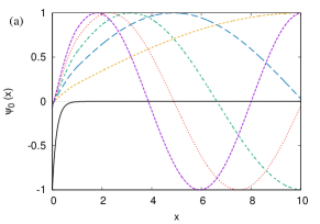
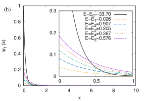
Figure 1: Wave functions (a) $\psi_{0}(x)$ and (b) $\psi_{1}(x)$ for the six lowest-lying-energy states with the TBC.

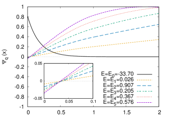
Figure 2: Nambu-Bethe-Salpeter wave functions $\Psi_{q}(x)=\psi_{0}(x)+q\psi_{1}(x)$ with $q=+0.2$. For better visibility, we inverted the sign of the NBS wave function for $E=E_{0}$ (since the overall normalization is irrelevant) and altered the $x$-range from Fig. 1.

IV.3 Non-Local Potentials

In Fig. 3, we show the regular part of the HAL QCD potentials $V^{(N)}(x,x^{\prime})$ and their expansion coefficients $\tilde{v}_{n}(x)$ at truncation orders $N=1,2,3,4,$ and $5$. The field admixture parameter and the Gaussian expansion scale are fixed to $q=0.2$ and $\rho=0.5$, respectively. The discontinuous structure seen in the potentials at $|x|=R=1$ is due to the edge of the square-well potential in the Birse model. The strength $g_{n}$ of their singular parts are summarized in Table 1.

We observe that the functional structure of the non-local potentials is not stable against the variation of $N$ as the magnitude of the potential tends to become larger for larger $N$. In principle, a potential is an off-shell object and variance in its functional structure itself does not necessarily imply that the expansion fails.

Unlike in Ref. Birse:2012ph , there is no repulsive behavior in the small $|x|$ region. In Ref. Birse:2012ph , the leading order potential of the naïve derivative expansion (15) is computed from a single NBS wave function of the first excited state. As we have seen in Fig. 2, the NBS wave function of the first excited state has a node at short distance. At that point the HAL QCD potential with the leading order derivative expansion diverges, and it looks as if there were a repulsive core. To avoid such superficial divergence, two or more NBS wave functions should be picked up from the lowest energy without omission to solve the matrix Eq. (24) for $(v_{0}(x),\cdots,v_{N}(x))^{T}$. In this case, the condition $\Phi_{\rho}(x;E_{i})=0$ for some combination of $x$ and $E_{i}$ does not necessarily mean that the inversion of the whole matrix fails in solving Eq. (24). We can thus obtain a smooth potential even at the nodal position.

In Fig. 4, we plot the following quantity for $N=1,\cdots,5$ to see the range of the potentials:

$$f^{(N)}(x)\equiv\underset{x^{\prime}}{\mbox{max}}\left|V^{(N)}(x,x^{\prime})\right|.$$ (32)

It is clear that $f^{(N)}(x)\simeq 0$ for $x>3$. In the calculation of the phase shift from the Lippmann-Schwinger equation below, we safely regard $V^{(N)}(x,x^{\prime})=0$ for $|x|>4$.

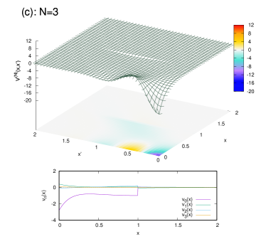
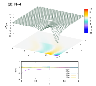
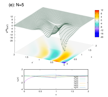
Figure 3: Regular part of the non-local HAL QCD potentials $V^{(N)}(x,x^{\prime})$ and their expansion coefficients $v_{n}(x)$ ($n=0,\cdots,N$) with $\rho=0.5$ and $q=0.2$. Panels (a), (b), (c), (d), and (e) show the results of $N=1,2,3,4,$ and $5$, respectively.

Table 1: Singular part strength $g_{n}$ of the potentials in Fig. 3.

$N$	$g_{0}$	$g_{1}$	$g_{2}$	$g_{3}$	$g_{4}$	$g_{5}$
$1$	$-16.31$	$5.58$
$2$	$-12.26$	$2.32$	$-1.47$
$3$	$-9.46$	$1.51$	$-0.46$	$0.48$
$4$	$-6.85$	$1.00$	$-0.19$	$0.05$	$-0.19$
$5$	$-4.20$	$0.54$	$-0.05$	$-0.03$	$0.04$	$0.09$

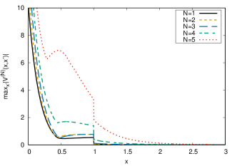
Figure 4: Function $f^{(N)}(x)$ with $\rho=0.5$ and $q=0.2$. (See Eq. (32))

IV.4 Scattering Phase Shift

IV.4.1 Convergence of the derivative expansion ($N$ dependence)

In Fig. 5, we show the scattering phase shifts extracted from the HAL QCD potentials with truncation orders $N=1,\cdots,5$. (Here we refer to these results as $\delta_{N}(E)$.) In order to make discussion clear, we show $\delta_{N}(E)$ only at the energies corresponding to the discrete eigenenergies of the Birse model solutions in the box , i.e., $E=E_{1},\cdots,E_{15}$. The field admixture parameter and the expansion scale are fixed to $q=0.2$ and $\rho=0.5$, respectively, so that the HAL QCD potentials correspond to the ones shown in Fig. 3. The results are compared to the exact values $\delta_{exact}(E)$ extracted from the analytic solution of the coupled-channel Eqs. (9). (Refer to Appendix D.2 for the explicit expression.) We see that, at each truncation order $N$, $\delta_{N}$ agrees with $\delta_{exact}$ at small energies, but deviates away at higher energies. However, the deviation tends to become smaller as $N$ increases. This observation supports that the generalized derivative expansion converges in terms of the phase shifts extracted from the non-local potentials.

It is helpful to discuss the energy dependence in $\delta_{N}$ through the following classification of the energy region. First, we see that each of the results of $\delta_{N}$ in Fig. 5 shows excellent agreement with $\delta_{exact}$ at discrete energies $E=E_{1},\cdots,E_{N}$. The agreement is ensured by construction, since the corresponding NBS wave functions are used as input. We also find that agreement holds in the intermediate intervals $E_{1}<E<E_{2},\cdots,E_{N-1}<E<E_{N}$. We refer to the entire $E\leq E_{N}$ interval as the “input region”. Secondly, we can see from Fig. 5 that agreement between $\delta_{N}$ and $\delta_{exact}$ extends beyond the input region up to some point. The agreement indicates that extrapolation to higher energy in terms of the phase shift is possible. We refer to such a region with nontrivial agreement as the “extrapolation region”.

In order to discuss the validity of truncation in the derivative expansion, the length of the extrapolation region is of question. From Fig. 5, we can see that at $N=1,2,3,4,$ and $5$, the results show extrapolated agreement in the intervals $E_{1}<E<E_{3}$ ($0.03\Delta$), $E_{2}<E<E_{8}$ ($0.24\Delta$), $E_{3}<E<E_{11}$ ($0.45\Delta$), $E_{4}<E<E_{12}$ ($0.51\Delta$), and $E_{5}<E<E_{13}$ ($0.58\Delta$), respectively, where the numbers in the parentheses are their lengths. This observation reconfirms the convergence of the expansion, as higher truncation order results in the extension of not only the input region, but of the extrapolation region, i.e., more robust extrapolation to higher energy.

Note that our phase shifts satisfy $\delta(E=0)=\pi/2$ in the 1+1 dimensional space-time with a single bound state, which is contrasted to $\delta_{l}(E=0)-\delta_{l}(E=\infty)=n_{l}\pi$ in 1+3 dimension, with $n_{l}$ being the number of bound states of angular momentum $l$.

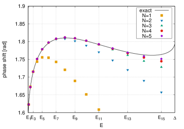
Figure 5: Scattering phase shift $\delta_{N}$ against energy $E$ at $N=1,\,2,\,3,\,4,\,$ and $5$, with fixed $\rho=0.5$ and $q=0.2$. The solid line represents the exact values extracted from the analytic solution of the Birse model (similarly in Fig. 6 and Fig. 7).

IV.4.2 Interpolating field dependence ($q$ dependence)

To discuss the dependence on the choice of interpolating fields, we vary the field admixture parameter as $q=-1.0,-0.2,+0.2,+1.0$, while the Gaussian expansion scale is fixed to $\rho=0.5$. Figure 6 shows the $q$ dependence of the scattering phase shift at truncation orders $N=2$ and $N=3$.

At $N=2$, clear $q$ dependence can be seen; for $E>E_{5}$, the phase shifts behave in a distinguishable manner. The $q$ dependence is smaller at $N=3$, where the variance in $\delta_{N}(E)$ against $q$ is smaller than at $N=2$ and all of the results show better agreement with the exact curve. By further increasing $N$ (despite the corresponding figures being omitted to save the space), we observe increasingly smaller $q$ dependence in the phase shifts. This implies that the generalized derivative expansion converges regardless of the choice of interpolating fields.

To look into how the convergence is affected by the variance in $q$, we first look at the results with $q=-1.0$. The extrapolation regions with $q=-1.0$ correspond to $E_{2}<E<E_{5}$ at $N=2$, and $E_{3}<E<E_{8}$ at $N=3$.

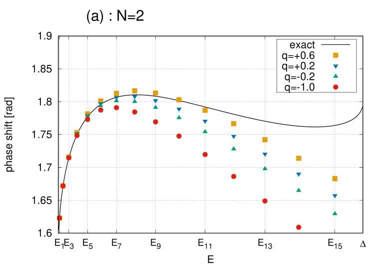
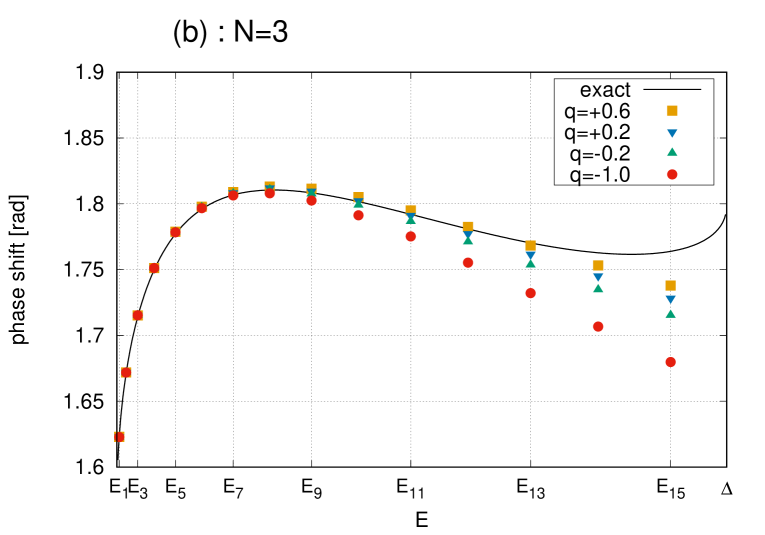
Figure 6: Scattering phase shift for $q=0.6,\,0.2,\,-0.2,\,-1.0$ with fixed $\rho=0.5$ at (a) $N=2$ and (b) $N=3$.

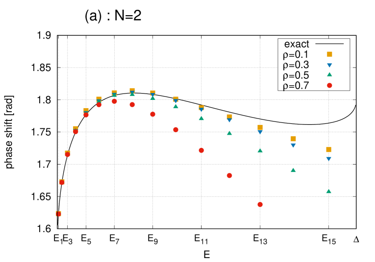
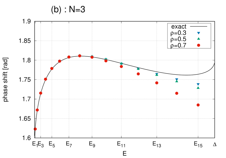
Figure 7: Scattering phase shift for (a) $\rho=0.1,\,0.3,\,0.5,\,0.7$ at $N=2$ and (b) $\rho=0.3,\,0.5,\,0.7$ at $N=3$. In both panels the field admixture parameter is fixed to $q=0.2$.

The extension of the extrapolation region reconfirms the above-mentioned convergence of the expansion. In comparison to these results, we take the case of $q=+0.2$ to find that the extrapolation regions are $E_{2}<E<E_{8}$ at $N=2$, and $E_{3}<E<E_{11}$ at $N=3$. It is observed that the lengths of the extrapolation regions are comparable between the results with $(q,N)=(+0.2,\,2)$ and $(q,N)=(-1.0,\,3)$ despite the different truncation orders. It indicates that the interpolating field corresponding to $q=+0.2$ results in better convergence than the one corresponding to $q=-1.0$. We therefore observe that the convergence of the generalized derivative expansion is improved by properly choosing interpolating fields. Among the four $q$ values employed here, $q=+0.2$ seems to be the best choice.

IV.4.3 Dependence on the Gaussian expansion scale $\rho$

It is expected that the convergence of the generalized derivative expansion can be improved by setting the expansion scale to the intrinsic non-locality size of HAL QCD potentials, as well as tuning the choice of interpolating fields. To see this, we vary the expansion scale $\rho$ while the field admixture is fixed to $q=+0.2$. In Fig. 7(a), we show the phase shifts obtained from HAL QCD potentials with $\rho=0.1,0.3,0.5$, and $0.7$ at truncation order $N=2$. Similarly, Fig. 7(b) shows the phase shifts with $\rho=0.3,0.5,0.7$ at $N=3$.

Let us compare the result with $(\rho,N)=(0.3,\,2)$ in Fig. 7(a) and that with $(\rho,N)=(0.7,\,3)$ in Fig. 7(b). In the former case, the extrapolation region extends to $E_{2}<E<E_{10}$, whereas that in the latter case corresponds to $E_{3}<E<E_{10}$. Since both cases with different truncation orders allow for extrapolation to comparable extrapolation regions, we conclude that a proper choice of the Gaussian expansion scale can improve the convergence of the generalized derivative expansion.

IV.5 Criteria for Convergence

The non-local potentials with $\rho=0.3$ and $0.7$ are shown in Fig. 8 with $N=3$ and $q=+0.2$ being fixed. Although their structures seem to be quite different, these two potentials reproduce the scattering phase shift quite well in the energy region $E\leq E_{9}$ (See Fig. 7(b)). Note that $E=E_{9}$ belongs to the extrapolation regions for both of these two parameter sets.

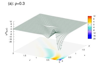
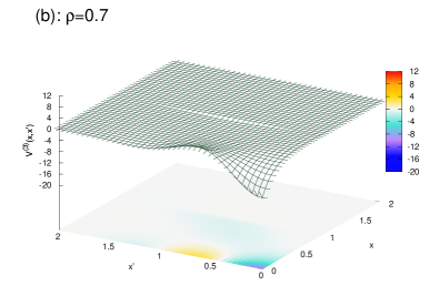
Figure 8: Non-local potentials $V^{(N)}(x,x^{\prime})$ with (a) $\rho=0.3$ and (b) $\rho=0.7$, at truncation order $N=3$. The field admixture parameter is fixed to $q=+0.2$ in both panels.

It may be of interest how the wave functions behave in the extrapolation region. We show the NBS wave functions at $E=E_{9}$ obtained from the two potentials together with the exact one in Fig. 9. We see that, while they agree at long distance, they show small deviation from the exact one at short distance of $x\lesssim 0.5$. The short-distance deviation is natural because the NBS wave function at $E=E_{9}$ is not used as input to construct these potentials, although the agreement in the phase shift ensures the correct long-distance behavior of the NBS wave functions.

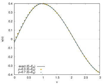
Figure 9: NBS wave functions at $E=E_{9}$ obtained with the two non-local potentials in Fig. 8 (i.e., the ones with $\rho=0.3$ and $\rho=0.7$, with fixed $q=+0.2$ and $N=3$) together with the analytic solution of the NBS wave function for comparison.

The difference in the structures between the two potentials in Fig. 8 indicates that the HAL QCD potential may not be uniquely determined as far as we use the NBS wave functions for a restricted energy region. This may be also the case even if we use all the NBS wave functions in the energy region $E\leq\Delta$. From these considerations, we learn that the stability in non-local potentials is too strict as a criterion for the convergence of the (generalized) derivative expansion. Physical observables, such as the phase shift will be more useful for that purpose.

V CONCLUSION

We have investigated general properties of the non-local potentials which HAL QCD collaboration introduced as wave function equivalent potentials. An analytically solvable coupled-channel model has been employed in order to implement the derivative expansion to higher orders explicitly. We have introduced a generalized derivative expansion to avoid a problem which arises when the naïve derivative expansion is applied to the present model due to its unsmooth NBS wave functions. The convergence of the new expansion has been studied numerically.

We have observed that the generalized derivative expansion of the non-local potentials converges quite well such that proper scattering phase shift is extracted, although the functional structure of the potentials is not uniquely determined. In addition to the energy region where the agreement of the phase shift is ensured by construction, the agreement extends to the higher energies, suggesting that the extrapolation of the phase shift by the generalized derivative expansion works successfully. Moreover, we have observed that the convergence is improved by properly choosing interpolating fields (the field admixture parameter $q$) and/or the Gaussian expansion scale ($\rho$) in the generalized derivative expansion.

Appendix A ADDITIONAL COMMENTS ON GENERALIZED DERIVATIVE EXPANSION

A.1 Derivation of Generalized Derivative Expansion

A general potential $V(x_{1},x_{2})\equiv\Braket{x_{1}}{V}{x_{2}}$ is reparameterized in the coordinate space and in the momentum space as

$$\begin{split}{\mathcal{V}}(R,r)&\equiv\Braket{x_{1}}{V}{x_{2}},\\ \tilde{\mathcal{V}}(k,P)&\equiv\Braket{p_{1}}{V}{p_{2}},\end{split}$$ (33)

respectively, where the coordinates $r$ and $R$, and the momenta $k$ and $P$ are defined as

$$\begin{split}r=x_{1}-x_{2},&\hskip 10.0ptR=x_{1},\\ k=p_{1}-p_{2},&\hskip 10.0ptP=p_{2}.\end{split}$$ (34)

The two representations in Eqs. (33) are related to each other via the Fourier transformation

$${\mathcal{V}}(R,r)=\iint\frac{dkdP}{2\pi}e^{ikR}\,\tilde{\mathcal{V}}(k,P)\,e^{iPr}.$$ (35)

First we derive the naïve derivative expansion (15). For this purpose, we replace all the $P$ dependence in $\tilde{\mathcal{V}}(k,P)$ by $\hat{P}=-i\partial/\partial r$, and then complete the integration over $P$ to have

$${\mathcal{V}}(R,r)={\mathcal{U}}_{0}(R,-i\partial/\partial r)\,\delta(r),$$ (36)

where

$${\mathcal{U}}_{0}(R,-i\partial/\partial r)\equiv\int dk\,e^{ikR}\,\tilde{\mathcal{V}}(k,-i\partial/\partial r).$$ (37)

We expand ${\mathcal{U}}_{0}(R,-i\partial/\partial r)$ as a power series of the derivative $\partial/\partial r$. To respect the time-reversal symmetry, ${\mathcal{V}}(R,r)$ have to be real-valued. Hence the power series is real at each order, and we have

$${\mathcal{U}}_{0}(R,-i\partial/\partial r)=\sum_{n=0}^{\infty}u_{n}(R)\left(\frac{\partial}{\partial r}\right)^{n},$$ (38)

which leads to the (naïve) derivative expansion formula:

$$V(x_{1},x_{2})=\sum_{n=0}^{\infty}u_{n}(x_{1})\left(\frac{\partial}{\partial x_{1}}\right)^{n}\delta(x_{1}-x_{2}).$$ (39)

Derivation of the generalized derivative expansion starts from factorizing the momentum-space representation $\tilde{\mathcal{V}}(k,P)$ according to

$$\tilde{\mathcal{V}}(k,P)\equiv\tilde{\mathcal{V}}_{\rho}(k,P)\exp\left\{-\frac{1}{4}\rho^{2}P^{2}\right\},$$ (40)

where an arbitrary real parameter $\rho$ is introduced. This time, the P dependence of the function $\tilde{\mathcal{V}}_{\rho}(k,P)$ is replaced by $\hat{P}=-i\partial/\partial r$, while that of the Gaussian function is left unchanged. Completing the integration of $P$ in Eq. (35), we have

$${\mathcal{V}}(R,r)={\mathcal{U}}_{\rho}(R,-i\partial/\partial r)\delta_{\rho}(r),$$ (41)

where

$${\mathcal{U}}_{\rho}(R,-i\partial/\partial r)\equiv\int dk\,e^{ikR}\tilde{\mathcal{V}}_{\rho}(k,-i\partial/\partial r),$$ (42)

and $\delta_{\rho}(r)$ is defined in Eq. (17). Again the time-reversal symmetry implies real-valued coefficients of ${\mathcal{U}}_{\rho}(R,-i\partial/\partial r)$ in the power-series expansion of $\partial/\partial r$, leading to the generalized derivative expansion

$$V(x_{1},x_{2})=\sum_{n=0}^{\infty}v_{n}^{(\rho)}(x_{1})\left(\frac{\partial}{\partial x_{1}}\right)^{n}\delta_{\rho}(x_{1}-x_{2}).$$ (43)

A.2 Need for replacement $\partial/\partial x\to\partial/\partial(x^{2})$

We consider the generalized derivative expansion with the conventional derivatives $\partial/\partial x,\,\partial^{2}/\partial x^{2},\cdots$. The Schrödinger equations for $N+1$ energy levels are expressed in a matrix form as

$${\bf u}(x)=M(x){\bf v}(x),$$ (44)

with

$${\bf u}(x) \equiv\left(\begin{array}[]{c}(E_{0}-H_{0})\Psi(x;E_{0})\\ (E_{1}-H_{0})\Psi(x;E_{1})\\ \vdots\\ (E_{N}-H_{0})\Psi(x;E_{N})\end{array}\right),$$ (49)

$$M(x) \equiv\left(\begin{array}[]{cccc}\Phi_{\rho}(x;E_{0})&\partial_{x}\Phi_{\rho}(x;E_{0})&\cdots&\partial_{x}^{N}\Phi_{\rho}(x;E_{0})\\ \Phi_{\rho}(x;E_{1})&\partial_{x}\Phi_{\rho}(x;E_{1})&\cdots&\partial_{x}^{N}\Phi_{\rho}(x;E_{1})\\ \vdots&\vdots&\ddots&\vdots\\ \Phi_{\rho}(x;E_{N})&\partial_{x}\Phi_{\rho}(x;E_{N})&\cdots&\partial_{x}^{N}\Phi_{\rho}(x;E_{N})\\ \end{array}\right),$$ (54)

$${\bf v}(x) \equiv\left(\begin{array}[]{c}v_{0}(x)\\ v_{1}(x)\\ \vdots\\ v_{N}(x)\end{array}\right),$$ (59)

where the summation over $n$ in the generalized derivative expansion (18) is truncated at order $N$. Equation (44) is solved for ${\bf v}(x)$ by inverting $M(x)$ point-by-point.

As far as the even-parity sector is considered, the smoothed wave function $\Phi_{\rho}(x;E)$ behaves as

$$\Phi_{\rho}(x;E)=\sum_{l=0}^{\infty}C_{l}(E)x^{2l}$$ (60)

around $x=0$, and its $k$-th order derivative reads

$$(\partial_{x})^{k}\Psi_{\rho}(x;E)=\sum_{l=0}^{\infty}C_{l}(E)\cdot(\partial_{x})^{k}x^{2l}.$$ (61)

If $k$ is odd, $(\partial_{x})^{k}\Psi_{\rho}(x;E)$ is of $\mathcal{O}(x)$, so that the even-numbered columns of $M(x)$ vanish at $x=0$. Hence the inversion of $M(x)$ fails and the coefficients ${\bf v}(x)$ diverges at $x=0$. For numerical calculations, such superficial divergence should be removed explicitly.

This problem can be avoided when basis $\left(\partial/\partial x\right)^{k}$ are replaced by $\left(\partial/\partial(x^{2})\right)^{k}$ ($k=0,1,\cdots$). The two basis are related to each other by linear transformation

$$\left(\frac{\partial}{\partial(x^{2})}\right)^{n}=\sum_{m=0}^{n}\alpha_{nm}(x)\frac{\partial^{m}}{\partial x^{m}},$$ (62)

where

$$\begin{split}a_{nm}(x)&\equiv a_{nm}/x^{2n-m}\hskip 20.00003pt\mbox{for }n\geq 0,\\ a_{0m}&\equiv\left\{\begin{array}[]{lcl}1&\mbox{for}&m=0\\ 0&\mbox{for}&m\neq 0\end{array}\right.,\\ a_{1m}&\equiv\left\{\begin{array}[]{lcl}1/2&\mbox{for}&m=1\\ 0&\mbox{for}&m\neq 1\end{array}\right.,\\ a_{n+1,m}&\equiv\frac{a_{n,m-1}}{2}+\frac{m-2n}{2}a_{n,m}\hskip 20.00003pt\mbox{for }n\geq 1.\end{split}$$ (63)

Since $\alpha_{nm}(x)$ thus defined is a lower triangular matrix with diagonal entries $\alpha_{nn}(x)=1/(2x)^{n}$, $\alpha(x)$ is invertible for $0<|x|<\infty$. Hence, Eq. (44) is equivalent to

$${\bf u}(x)=\tilde{M}(x)\tilde{\bf v}(x),$$ (64)

where

$$\tilde{M}(x) \equiv M(x)\alpha(x)^{T},$$ (65)

$$\tilde{\bf v}(x) \equiv \left(\begin{array}[]{c}\tilde{v}_{0}(x)\\ \tilde{v}_{1}(x)\\ \vdots\\ \tilde{v}_{N}(x)\end{array}\right)\equiv(\alpha(x)^{T})^{-1}{\bf v}(x).$$ (70)

Notice that Eq. (64) is nothing but the Schrödinger equations with the generalized derivative expansion where the conventional derivatives $\partial/\partial x$ are replaced by $D_{x}\equiv\partial/\partial(x^{2})$. Although ${\bf v}(x)$ are singular at $x=0$, linear combination (70) cancels terms with negative powers of $x$, leaving singularity-free coefficients $\tilde{\bf v}(x)$. The replacement $\left(\partial/\partial x\right)^{n}\to\left(\partial/\partial(x^{2})\right)^{n}$ rearranges the coefficients but does not change the non-local potential $V^{(N)}(x,x^{\prime})$.

We take the $N=2$ case as an example. Matrix $\alpha(x)$ in this case is given as

$$\alpha(x)=\begin{pmatrix}1&0&0\\ 0&\frac{1}{2x}&0\\ 0&-\frac{1}{4x^{3}}&\frac{1}{4x^{2}}\end{pmatrix},$$ (71)

which leads to

$$\begin{split}\frac{\partial}{\partial(x^{2})}&=\frac{1}{2x}\frac{\partial}{\partial x},\\ \frac{\partial^{2}}{\partial(x^{2})^{2}}&=-\frac{1}{4x^{3}}\frac{\partial}{\partial x}+\frac{1}{4x^{2}}\frac{\partial^{2}}{\partial x^{2}}.\end{split}$$ (72)

The relation between ${\bf v}(x)$ and $\tilde{\bf v}(x)$ then reads

$$\begin{split}\tilde{v}_{0}(x)&=v_{0}(x),\\ \tilde{v}_{1}(x)&=2xv_{1}(x)+2v_{2}(x),\\ \tilde{v}_{2}(x)&=4x^{2}v_{2}(x),\end{split}$$ (73)

so that negative powers of $x$ in ${\bf v}(x)$ are all cancelled in $\tilde{\bf v}(x)$.

Appendix B Need for Twisted Boundary Condition

We consider the Schrödinger Eqs. (44) with the generalized derivative expansion of the conventional derivatives $\partial_{x},(\partial_{x})^{2},\cdots$, in the interval $-L<x<+L$. Note that, in the even-parity sector, the following relation is satisfied:

$$[(\partial_{x})^{k}\Phi_{\rho}](-x;E)=\left\{\begin{array}[]{lcl}+[(\partial_{x})^{k}\Phi_{\rho}](x;E)&\mbox{for}&\mbox{even }k\\ -[(\partial_{x})^{k}\Phi_{\rho}](x;E)&\mbox{for}&\mbox{odd }k\end{array}\right.$$ (74)

Now, suppose that the periodic boundary condition (PBC) is imposed on the wave functions:

$$\Phi_{\rho}(x+2L;E)=\Phi_{\rho}(x;E).$$ (75)

Conditions (74) and (75) imply

$$(\partial_{x})^{k}\Phi_{\rho}(x=L;E)=0\hskip 20.00003pt\mbox{for odd }k$$ (76)

at any energy. Thus the even-numbered columns of the matrix $M(x)$ vanish at $x=\pm L$ so that $M(x)$ is not invertible. A similar problem arises when the anti-periodic boundary condition (APBC) is imposed such that

$$\Phi_{\rho}(x+2L;E)=-\Phi_{\rho}(x;E).$$ (77)

In this case the odd-numbered columns of $M(x)$ containing even-order derivatives vanish, and $M(x)$ is uninvertible.

The above argument also holds when the conventional derivatives $\left(\partial/\partial x\right)^{n}$ are replaced by $D_{x}^{n}$, since the relation $\mbox{det}(\tilde{M}(x))=\mbox{det}(M(x))\mbox{det}(\alpha(x))$ implies that $\tilde{M}(x)$ is uninvertible if $\mbox{det}M(x)=0$.

With large enough $L$, the potential is expected to become negligibly small near the boundary. However, as far as $L$ is finite, non-invertible nature of $M(x)$ is still troublesome for numerical determination of the potential. Although the origin of the problem is similar to the one considered in Appendix A.2, we do not employ similar strategy, because it results in unwanted $L$ dependence in the potential.

An alternative solution is to impose the twisted boundary conditions (30) with $\theta=\pi/2$. With this boundary condition, the even-parity solution (the real part) is smoothly connected with the odd-parity solution (the imaginary part) at the boundary. The derivatives of $\Phi_{\rho}(x;E)$ vanish only accidentally and $E$-dependently, so that $M(x)$ is safely invertible at $x=\pm L$.

Appendix C Zero-Determinant Problem

So far we have discussed the cases where the matrix inversion in Eq. (24) is safely taken. We have introduced the generalized derivative expansion since the Birse model wave functions are not smooth at $x=\pm R$, i.e., at the edge of the square-well potential. The $x^{2}$-derivative operator $D=\partial/\partial(x^{2})$ and the TBC have been employed to avoid the problems at $x=0$ and $x=\pm L$, respectively. Each of these problems happens at a specific point in space and can be explicitly avoided; however, in some cases an additional problem arises at accidental points, which should be overcome one-by-one by another technique.

The quantity of central importance is the determinant

$$\mbox{det}M(x;q)=\mbox{det}\begin{pmatrix}\Phi_{q}(x;E_{0})&\cdots&D^{N}\Phi_{q}(x;E_{0})\\ \vdots&\ddots&\vdots\\ \Phi_{q}(x;E_{N})&\cdots&D^{N}\Phi_{q}(x;E_{N})\end{pmatrix}.$$ (78)

Let us suppose that the matrix $M$ is invertible in the whole spatial region when we take $q=q_{0}$, i.e.

$$h_{0}(x)\equiv\mbox{det}M(x;q_{0})\neq 0\hskip 20.00003pt\mbox{for all }x.$$ (79)

We then try to improve the convergence of the generalized derivative expansion by changing the field admixture parameter by $\delta q\equiv q-q_{0}$, so that the NBS wave function reads

$$\Phi_{q}(x)=\Phi_{q_{0}}(x)+\delta q\phi_{1}(x),$$ (80)

where $\phi_{1}(x)\equiv\int dx^{\prime}\delta_{\rho}(x-x^{\prime})\psi_{1}(x^{\prime})$, the Gaussian-smoothed function of $\psi_{1}(x)$, behaves in the qualitatively same way as $\psi_{1}(x)$ itself, i.e., $\phi_{1}(x)\sim e^{-\gamma|x|}$. By substituting Eq. (80) in Eq. (78), we find that the determinant is in general expressed as an (N+1)-th order polynominal of $\delta q$:

$$\mbox{det}M(x;q)=h_{0}(x)+h_{1}(x)\delta q+\cdots+h_{N+1}(x)(\delta q)^{N+1}.$$ (81)

The functions $h_{n}(x)$ ($n=0,\cdots,N+1$) are all real and continuous in $x$, each of which involves n-fold product of $\phi_{1}(x)$ and/or their derivatives. Recalling that $\psi_{1}(x)$ (and thus $\phi_{1}(x)$) vanishes exponentially at large distance, we find

$$\mbox{det}M(x;q)\simeq h_{0}(x),$$ (82)

for large enough $x$, so that the matrix $M(x;q)$ is invertible. On the other hand, Eq. (82) cannot be satisfied for small $x$, where the higher-order terms in Eq. (81) give non-vanishing contribution. In principle, in some cases of $\delta q\neq 0$, there might be one (or more) small $x$ where the determinant satisfies $\mbox{det}M(x;q)=0$. These zeros result in singular behavior in the coefficients of the derivative expansion, $v_{n}(x)$, as we have discussed before. The choice of $q$ value is restricted to a certain region to avoid this problem, and the allowed region shall in general be smaller for larger truncation order $N$, since the dependence in $q$ becomes greater in Eq. (81).

The same argument is also valid in lattice QCD. We consider constructing the HAL QCD potential for a system of two hadrons, $H_{A}$ and $H_{B}$. By using local interpolating fields $\hat{A}_{0}$ for $H_{A}$ and $\hat{B}$ for $H_{B}$, we define the NBS wave function $\Psi_{0}({\bm{x}})$ as

$$\Psi_{0}({\bm{x}})\equiv\Braket{0}{\hat{A}_{0}({\bm{x}}+{\bm{y}})\hat{B}({\bm{y}})}{\Psi}.$$ (83)

Meanwhile, we try to improve the convergence of the derivative expansion by arranging the coupling of operator $\hat{A}_{0}$ to the excited states of $H_{A}$ in the following way. We first take a linear combination of $\hat{A}_{0}$ and another interpolating field $\hat{A}_{1}$ for $H_{A}$ to construct an operator $\hat{A}^{\prime}$, which does not couple to the lowest-energy state of the quantum numbers of $H_{A}$, $\ket{H_{A};ground}$:

$$\Braket{0}{\hat{A}^{\prime}}{H_{A};ground}=0.$$ (84)

It is used to compose a new interpolating field

$$\hat{A}_{r}\equiv\hat{A}_{0}+r\hat{A}^{\prime},$$ (85)

with arbitrary parameter $r$. We obtain the NBS wave function $\Psi_{r}({\bm{x}})$ with interpolating fields $\hat{A}_{r}$ and $\hat{B}$,

$$\Psi_{r}({\bm{x}})\equiv\Braket{0}{\hat{A}_{r}({\bm{x}}+{\bm{y}})\hat{B}({\bm{y}})}{\Psi},$$ (86)

which asymptotically approaches $\Psi_{0}({\bm{x}})$, since the admixture of $\hat{A}^{\prime}$ is suppressed at large distance. By comparing $\Psi_{0}({\bm{x}})$ and $\Psi_{r}({\bm{x}})$ to the NBS wave functions in the previous argument with $q=q_{0}$ and $q=q_{0}+r$, respectively, we find that the same problem can also occur in the lattice QCD cases.

There is a way to overcome the problem in virtue of the introduction of the generalized derivative expansion. Recall the fact that the functional form of the non-local potential varies depending on the expansion scale $\rho$. Variance in $\rho$ can shift the zeros of $\mbox{det}M(x;\rho)$ (here we explicitly indicate the $\rho$ dependence of $M$) as

$$\begin{split}\mbox{det}M(x=a_{1};\rho_{1})=0&\to\mbox{det}M(x=a_{2};\rho_{2})=0,\\ a_{1}\neq a_{2},&\hskip 4.0pt\rho_{1}\neq\rho_{2}.\end{split}$$ (87)

Moreover, if we determine more than two non-local potentials $V^{(\rho)}(x,x^{\prime})$ with different choices of $\rho$ from the same $(N+1)$ NBS wave functions, all of those potentials manifestly reproduce the input NBS wave functions. It means that, $V^{(\rho)}(x,x^{\prime})$ acts in the same way on $\Psi(x;E)$ for $E\leq E_{N}$, regardless of $\rho$. Then it follows that a weighted average of the potentials

$$\overline{V}(x,x^{\prime}) \equiv\int d\rho\,w(x;\rho)V^{(\rho)}(x,x^{\prime}),$$ (88)

$$\int d\rho\,w(x;\rho)=1,$$ (89)

also reproduces the correct NBS wave functions for these energies. Note that the weight function $w(x;\rho)$ can be chosen totally arbitrarily as far as the normalization condition (89) is satisfied.

To be more specific, let us consider the case indicated in Eq. (87), and assume that the corresponding non-local potentials $V^{(\rho_{1})}(x,x^{\prime})$ and $V^{(\rho_{2})}(x,x^{\prime})$ are obtained from the same NBS wave functions, despite being singular only at $x=a_{1}$ and $x=a_{2}$, respectively. We employ the weight function

$$w(x;\rho)=\lambda(x)\delta(\rho-\rho_{1})+(1-\lambda(x))\delta(\rho-\rho_{2}),$$ (90)

so that

$$\overline{V}(x,x^{\prime})=\lambda(x)V^{(\rho_{1})}(x,x^{\prime})+(1-\lambda(x))V^{(\rho_{2})}(x,x^{\prime}).$$ (91)

The function $\lambda(x)$ is taken to be smooth and to satisfy the conditions $\lambda(x)=0$ for $x\simeq a_{1}$ and $\lambda(x)=1$ for $x\simeq a_{2}$. Then the singularities at $x=a_{1}$ and $x=a_{2}$ are both stamped out, so that $\overline{V}(x,x^{\prime})$ is singularity-free. In actual calculations, the function $g(x)$ defined by

$$\begin{split}g(x)&\equiv f(x-a)/(f(x-a)+f(b-x)),\\ f(x)&\equiv\begin{cases}\exp(-1/x)&\mbox{for }x>0\\ 0&\mbox{for }x\leq 0\end{cases},\end{split}$$ (92)

will be useful to give $\lambda(x)$ a specific expression, which satisfies $g(x\leq a)=0$ and $g(x\geq b)=1$, and is smoothly connected in $a<x<b$.

By properly choosing the weight function $w(x;\rho)$, we can always remove all the singularities from the HAL QCD potential, while ensuring that it reproduces the correct NBS wave functions. The above argument also implies that we need special care in discussing the structure of a non-local potential, since a HAL QCD potential can be an artificial patchwork of arbitrary pieces of wave-function-equivalent potentials with different structures.

Appendix D Analytic Solutions

D.1 Solutions with TBC

Coupled-channel Eqs. (9) can be solved analytically in a finite spatial interval with TBC (30). Here we provide the exact expression of the solution, since it is rather complicated.

In energy region $0<E<\Delta$, the solution is given as:

$$\psi_{0}(x) =\begin{cases}(A\cos{\alpha x}+B\sin{\alpha|x|})+C\sin{\alpha x}&0<|x|<R\\ (D\cos{\beta x}+E\sin{\beta|x|})\\ \hskip 14.22636pt+(Fsgn(x)\cos{\beta x}+G\sin{\beta x}),&R<|x|<L\end{cases}$$

$$\psi_{1}(x) =(H\cosh{\gamma x}+I\sinh{\gamma|x|})+J\sinh\gamma x,$$ (93)

where $sgn(x)$ denotes the sign function

$$sgn(x)=\begin{cases}+1&x>0\\ 0&x=0\\ -1&x<0\end{cases}.$$ (94)

The associated momenta and the coefficients are given as follows.

$$\alpha\equiv\sqrt{M(E+V_{0})},\beta\equiv\sqrt{ME},\gamma\equiv\sqrt{M(\Delta-E)},$$ (95)

$$\begin{split}A&=(-iJ)\frac{\gamma}{Mg}(\cos\theta/\cosh{2\gamma L}-1),\allowdisplaybreaks\\ B&=(-iJ)\frac{Mg}{\alpha}\tanh{2\gamma L},\allowdisplaybreaks\\ C&=\frac{J}{\sin\theta}\frac{D_{0}\sinh{2\beta L}-E_{0}(\cos\theta+\cos{2\beta L})}{\sin{\alpha R}\sin{\beta R}+\frac{\alpha}{\beta}\cos{\alpha R}\cos{\beta R}},\allowdisplaybreaks\\ D&=(-iJ)D_{0},\allowdisplaybreaks\\ E&=(-iJ)E_{0},\allowdisplaybreaks\\ F&=\frac{J}{\sin\theta}\left(-D_{0}(\cos\theta-\cos{2\beta L})+E_{0}\sin{2\beta L}\right),\allowdisplaybreaks\\ G&=\frac{J}{\sin\theta}\left(D_{0}\sin{2\beta L}-E_{0}(\cos\theta+\cos{2\beta L})\right),\allowdisplaybreaks\\ H&=(-iJ)\tanh{2\gamma L},\allowdisplaybreaks\\ I&=(-iJ)(\cos\theta/\cosh{2\gamma L}-1),\end{split}$$ (96)

$$D_{0} =\frac{\gamma}{Mg}\left(\cos{\alpha R}\cos{\beta R}+\frac{\alpha}{\beta}\sin{\alpha R}\sin{\beta R}\right)\left(\frac{\cos\theta}{\cosh{2\gamma L}}-1\right)+\frac{Mg}{\alpha}\left(\sin{\alpha R}\cos{\beta R}-\frac{\alpha}{\beta}\cos{\alpha R}\sin{\beta R}\right)\tanh{2\gamma L},$$

$$E_{0} =\frac{\gamma}{Mg}\left(\cos{\alpha R}\sin{\beta R}-\frac{\alpha}{\beta}\sin{\alpha R}\cos{\beta R}\right)\left(\frac{\cos\theta}{\cosh{2\gamma L}}-1\right)+\frac{Mg}{\alpha}\left(\sin{\alpha R}\sin{\beta R}+\frac{\alpha}{\beta}\cos{\alpha R}\cos{\beta R}\right)\tanh{2\gamma L}.$$

The allowed energy eigenstates satisfy the relation

$$\mbox{det}\begin{pmatrix}+D_{0}(\cos\theta-\cos{2\beta L})-E_{0}\sin{2\beta L},&\sin{\alpha R}\cos{\beta R}-\frac{\alpha}{\beta}\cos{\alpha R}\sin{\beta R}\\ -D_{0}\sin{2\beta L}+E_{0}(\cos\theta+\cos{2\beta L}),&\sin{\alpha R}\sin{\beta R}+\frac{\alpha}{\beta}\cos{\alpha R}\cos{\beta R}\end{pmatrix}=0.$$ (97)

Be aware that, if we take the phase factor $J$ to be pure imaginary, i.e. $J=i$, the parity-even and the parity-odd parts are separated out.

We refrain from writing down the whole expressions for $-V_{0}<E<0$ and $E<-V_{0}$ to avoid redundancy. Instead, we note that the solution for $-V_{0}<E<0$ is obtained through replacement

$$\begin{split}\beta&\to\beta^{\prime}\equiv i\sqrt{-ME},\\ \cos{\beta x}&\to\cosh{\beta^{\prime}x},\\ \sin{\beta x}&\to i\sinh{\beta^{\prime}x},\end{split}$$ (98)

in each relevant quantity in Eqs. (93-97). For $E<-V_{0}$, further replacement

$$\begin{split}\alpha&\to\alpha^{\prime}\equiv i\sqrt{-M(E+V_{0})},\\ \cos{\alpha x}&\to\cosh{\alpha^{\prime}x},\\ \sin{\alpha x}&\to i\sinh{\alpha^{\prime}x}\end{split}$$ (99)

is necessary as well as replacement (98).

D.2 Scattering Phase Shift in the Infinite Volume

It is less time-consuming to solve the coupled-channel Eqs. (9) in the infinite volume. We give the exact expression of the scattering phase shift extracted from this analytic solution as follows:

$$\tan\delta_{exact}=\frac{\frac{\gamma}{Mg}\left(\cos{\alpha R}\sin{\beta R}-\frac{\alpha}{\beta}\sin{\alpha R}\cos{\beta R}\right)-\frac{Mg}{\alpha}\left(\sin{\alpha R}\sin{\beta R}+\frac{\alpha}{\beta}\cos{\alpha R}\cos{\beta R}\right)}{\frac{\gamma}{Mg}\left(\cos{\alpha R}\cos{\beta R}+\frac{\alpha}{\beta}\sin{\alpha R}\sin{\beta R}\right)-\frac{Mg}{\alpha}\left(\sin{\alpha R}\cos{\beta R}-\frac{\alpha}{\beta}\cos{\alpha R}\sin{\beta R}\right)}.$$ (100)

References

- (1) R. Machleidt, Phys. Rev. C 63, 024001 (2001) doi:10.1103/PhysRevC.63.024001 [nucl-th/0006014].
- (2) V. G. J. Stoks, R. A. M. Klomp, C. P. F. Terheggen and J. J. de Swart, Phys. Rev. C 49, 2950 (1994) doi:10.1103/PhysRevC.49.2950 [nucl-th/9406039].
- (3) R. B. Wiringa, V. G. J. Stoks and R. Schiavilla, Phys. Rev. C 51, 38 (1995) doi:10.1103/PhysRevC.51.38 [nucl-th/9408016].
- (4) E. Epelbaum, H. W. Hammer and U. G. Meissner, Rev. Mod. Phys. 81, 1773 (2009) doi:10.1103/RevModPhys.81.1773 [arXiv:0811.1338 [nucl-th]].
- (5) M. Luscher, Nucl. Phys. B 354, 531 (1991). doi:10.1016/0550-3213(91)90366-6
- (6) M. Fukugita, Y. Kuramashi, M. Okawa, H. Mino and A. Ukawa, Phys. Rev. D 52, 3003 (1995) doi:10.1103/PhysRevD.52.3003 [hep-lat/9501024].
- (7) S. R. Beane, P. F. Bedaque, K. Orginos and M. J. Savage, Phys. Rev. Lett. 97, 012001 (2006) doi:10.1103/PhysRevLett.97.012001 [hep-lat/0602010].
- (8) S. R. Beane, E. Chang, W. Detmold, H. W. Lin, T. C. Luu, K. Orginos, A. Parreño, M. J. Savage, A. Torok, and A. Walker-Loud [NPLQCD Collaboration], Phys. Rev. D 85, 054511 (2012) doi:10.1103/PhysRevD.85.054511 [arXiv:1109.2889 [hep-lat]].
- (9) S. R. Beane, E. Chang, S. D. Cohen, W. Detmold, H. W. Lin, T. C. Luu, K. Orginos, A. Parreño, M. J. Savage, and A. Walker-Loud [NPLQCD Collaboration], Phys. Rev. D 87, no. 3, 034506 (2013) doi:10.1103/PhysRevD.87.034506 [arXiv:1206.5219 [hep-lat]].
- (10) K. Orginos, A. Parreño, M. J. Savage, S. R. Beane, E. Chang and W. Detmold, Phys. Rev. D 92, no. 11, 114512 (2015) doi:10.1103/PhysRevD.92.114512 [arXiv:1508.07583 [hep-lat]].
- (11) T. Yamazaki, Y. Kuramashi, and A. Ukawa [PACS-CS Collaboration], Phys. Rev. D 84, 054506 (2011) doi:10.1103/PhysRevD.84.054506 [arXiv:1105.1418 [hep-lat]].
- (12) T. Yamazaki, K. i. Ishikawa, Y. Kuramashi and A. Ukawa, Phys. Rev. D 86, 074514 (2012) doi:10.1103/PhysRevD.86.074514 [arXiv:1207.4277 [hep-lat]].
- (13) T. Yamazaki, K. i. Ishikawa, Y. Kuramashi and A. Ukawa, Phys. Rev. D 92, no. 1, 014501 (2015) doi:10.1103/PhysRevD.92.014501 [arXiv:1502.04182 [hep-lat]].
- (14) E. Berkowitz, T. Kurth, A. Nicholson, B. Joo, E. Rinaldi, M. Strother, P. M. Vranas and A. Walker-Loud, arXiv:1508.00886 [hep-lat].
- (15) T. Iritani, T. Doi, S. Aoki, S. Gongyo, T. Hatsuda, Y. Ikeda, T. Inoue, N. Ishii, K. Murano, H. Nemura, and K. Sasaki [HAL QCD collaboration], JHEP 1610, 101 (2016) doi:10.1007/JHEP10(2016)101 [arXiv:1607.06371 [hep-lat]].
- (16) N. Ishii, S. Aoki and T. Hatsuda, Phys. Rev. Lett. 99, 022001 (2007) doi:10.1103/PhysRevLett.99.022001 [nucl-th/0611096].
- (17) S. Aoki, T. Hatsuda and N. Ishii, Prog. Theor. Phys. 123, 89 (2010) doi:10.1143/PTP.123.89 [arXiv:0909.5585 [hep-lat]].
- (18) N. Ishii, S. Aoki, T. Doi, T. Hatsuda, Y. Ikeda, T. Inoue, K. Murano, H. Nemura, and K. Sasaki [HAL QCD Collaboration], Phys. Lett. B 712, 437 (2012) doi:10.1016/j.physletb.2012.04.076 [arXiv:1203.3642 [hep-lat]].
- (19) S. Aoki, T. Doi, T. Hatsuda, Y. Ikeda, T. Inoue, N. Ishii, K. Murano, H. Nemura, and K. Sasaki [HAL QCD Collaboration], PTEP 2012, 01A105 (2012) doi:10.1093/ptep/pts010 [arXiv:1206.5088 [hep-lat]].
- (20) T. Kurth, N. Ishii, T. Doi, S. Aoki and T. Hatsuda, JHEP 1312, 015 (2013) doi:10.1007/JHEP12(2013)015 [arXiv:1305.4462 [hep-lat], arXiv:1305.4462].
- (21) K. Murano, N. Ishii, S. Aoki and T. Hatsuda, Prog. Theor. Phys. 125, 1225 (2011) doi:10.1143/PTP.125.1225 [arXiv:1103.0619 [hep-lat]].
- (22) M. C. Birse, arXiv:1208.4807 [nucl-th].
- (23) S. Aoki, M. Fukugita, K-I. Ishikawa, N. Ishizuka, Y. Iwasaki, K. Kanaya, T. Kaneko, Y. Kuramashi, M. Okawa, A. Ukawa, T. Yamazaki, and T. Yoshié [CP-PACS Collaboration], Phys. Rev. D 71, 094504 (2005) doi:10.1103/PhysRevD.71.094504 [hep-lat/0503025].
- (24) C. J. D. Lin, G. Martinelli, C. T. Sachrajda and M. Testa, Nucl. Phys. B 619, 467 (2001) doi:10.1016/S0550-3213(01)00495-3 [hep-lat/0104006].