Convergent Chaos

Abstract

Chaos is widely understood as being a consequence of sensitive dependence upon initial conditions. This is the result of an instability in phase space, which separates trajectories exponentially. Here, we demonstrate that this criterion should be refined. Despite their overall intrinsic instability, trajectories may be very strongly convergent in phase space over extremely long periods, as revealed by our investigation of a simple chaotic system (a realistic model for small bodies in a turbulent flow). We establish that this strong convergence is a multi-facetted phenomenon, in which the clustering is intense, widespread and balanced by lacunarity of other regions. Power laws, indicative of scale-free features, characterize the distribution of particles in the system. We use large-deviation and extreme-value statistics to explain the effect. Our results show that the interpretation of the ‘butterfly effect’ needs to be carefully qualified. We argue that the combination of mixing and clustering processes makes our specific model relevant to understanding the evolution of simple organisms. Lastly, this notion of convergent chaos, which implies the existence of conditions for which uncertainties are unexpectedly small, may also be relevant to the valuation of insurance and futures contracts.

I Introduction

The concept of ‘chaos’ is one of the most salient paradigms of modern science Ott02 . The significance of the central notion of exponential sensitivity to initial conditions is emblematically illustrated by the ‘butterfly effect’. The question “Does the flap of a butterfly’s wings in Brazil set off a tornado in Texas?” was famously posed by E. N. Lorenz in a conference talk in 1972 Lor72 ; Lor95 ; Pal+14 . In the roughly half century since Lorenz’s work, his question has invariably been conflated with: “Can the flap of a butterfly’s wings … ?” The affirmative answer to that question has cemented sensitive dependence on initial conditions as a hallmark of chaotic systems, the weather system included. But a deep, outstanding question behind the butterfly effect lies in Lorenz’s original formulation: Are perturbations destined to alter the course of large-scale patterns in turbulent systems? Or could regions of the phase space of a chaotic dynamical system be screened off from small perturbations? This is the real import of Lorenz’s Brazilian butterfly, and we note that Lorenz never definitively answered his original question.

It is the purpose of this paper to suggest an important and widely applicable refinement of the concept of chaos, based upon results illustrated by figure 1. This shows trajectories of particles in a model for the motion of particles in a turbulent fluid flow. In order to simplify the discussion we consider a one-dimensional model, where the position of a particle is $x(t)$ at time $t$. In this model, it has been proven that trajectories separate exponentially. In technical terms, the rate of separation of trajectories (the Lyapunov exponentOtt02 ) is positive. However, the trajectories illustrated in figure 1 show a strong tendency to cluster together, despite the fact that they must eventually diverge.

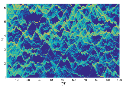
Figure 1: Trajectories, $x(t)$, for the dynamical system described by (II): many trajectories show strong and long lasting convergence, despite the fact that they must ultimately diverge. The colormap is chosen so that blue and yellow correspond to sparse and highly dense regions, respectively. Parameter values are quoted in the text. Clusters of trajectories can persist over durations long compared to the expected separation time, which, with the model used here, is $\approx 15/\gamma$.

In several one-dimensional chaotic systems, it has been observed that trajectories may show a temporary convergence preceding their eventual separation (see, for example Fuj83 , Aur+96 ). Figure 1 reveals that the convergence can lead to clusters of trajectories, over times which are much longer than the expected divergence time. Additionally, figure 1 reveals that the simulated trajectories tend to form surprisingly dense clusters. Quantitatively, for over $50\%$ of the time, $10\%$ of the $1.5\times 10^{4}$ trajectories used in figure 1 are clustered into a region of width $\Delta x=L/4000\approx 10^{-3}$, where $L=2\pi$ is the domain size. At some instants, up to $70\%$ of the total number of trajectories can accumulate in a region of size $L/4000$.

Thus, the phenomenon illustrated in Figure 1 indicates that, despite the intrinsic unpredictability of the system on very long time scales, there may be basins in the space of initial conditions which attract a significant fraction of the phase space over a finite time, giving a final position which is highly insensitive to the initial conditions. If the initial conditions which are of physical interest lie within one of these basins, the behaviour of the system can be computed accurately for a time which is many multiples of the inverse of the Lyapunov coefficient. The possibility of the butterfly effect is contained in the definition of chaos. Our results, however, indicate that the standard definition of chaos, dependent upon a positive Lyapunov exponent, does not necessarily imply a sensitive dependence upon initial conditions in practical applications, where we are only concerned with finite times.

In this paper we discuss various quantitative aspects of the clustering effect shown in figure 1. After introducing a canonical model in section II, we give a summary of our results on the strength of the effect (section III). When we examine the structure of the patterns in figure 1 statistically, we find (section IV) that power-law relations are ubiquitous, indicating scale-free behaviour with universal characteristics Strogatz:2001 . In section V we explain strong convergence effect quantitatively by considering the finite-time Lyapunov exponent. Using a combination of large-deviation and extreme-value statistics approaches, we have been able to show that the minimum value of the finite-time Lyapunov exponent can remain negative for a very long time. In section VI we argue that some trajectories may show perpetually convergent behaviour. The phenomena described in our studies are expected to be realised in a wide range of physically relevant models, and section VII discusses possible areas of application.

II A simple chaotic system

To stress the notion of intrinsic stochasticity in dynamical systems, the most intensively studied models for chaos are purely deterministic. For the purpose of understanding generic physical processes, however, these models may lead to the physically artificial situation where large regions of phase space are inaccessible at long time. In many extended physical systems, some degrees of freedom play a minor role, and can be modelled stochastically. In addition, dynamical models that contain random elements are less prone to lead to empty regions of phase space. These considerations provides a strong physical motivation to consider a dynamical model with random elements. In such a model, the emergence of sparse regions in phase space, as found e.g. in the case of inertial particles in turbulent flows Eaton+91 , necessarily results from a nontrivial dynamical property of the system.

We therefore propose to consider a model in which the trajectories have a continuous dependence upon the phase point, but where the dynamics contains random elements. In order to eliminate irrelevant details, it is also desirable to have a model for which statistics of the phase-space velocity are invariant under translations in time and space.

Among many possible abstract dynamical systems containing stochastic processes which satisfy these criteria, we have chosen a model which has a very direct physical interpretation, and which has already been extensively studied Fal+00 . The model that we consider is a realistic description of a ubiquitous physical phenomenon, namely the motion of small particles in a turbulent fluid. The equations of motion are Max+83 ; Gat83

$$\dot{x} = v,$$

$$\dot{v} = \gamma[u(x,t)-v].$$ (1)

Here $\gamma$ is a constant describing the rate of damping of motion of a small particle relative to the fluid and $u(x,t)$ is a randomly fluctuating velocity field of the fluid in which the particles are suspended. In figure 1 we solved (II) on the interval $[0,L]$ with periodic boundary conditions, and a velocity field where the correlation function is white noise in time, satisfying $\langle u(x,t)\rangle=0$ and $\langle u(x,t)u(x^{\prime},t^{\prime})\rangle=\delta(t-t^{\prime})C(x-x^{\prime})$, where angular brackets denote averages throughout. The correlation function is $C(\Delta x)=\epsilon^{2}\xi^{2}\gamma\,\exp\left(-\Delta x^{2}/2\xi^{2}\right)$, where $\xi$ is the correlation length and $\epsilon$ is a coupling constant. The numerical parameters were $L=2\pi$, $\xi=0.08$, $\gamma=0.0112$ and $\epsilon=1.25\,\epsilon_{c}$, where $\epsilon_{c}\approx 1.331$ is the value above which the Lyapunov exponent becomes positiveWil+03 .

The results obtained with model (II) for a simple $1$-dimensional system will be corroborated qualitatively by the results of a model of a compressible $2$-dimensional flow, presented in Section VII.

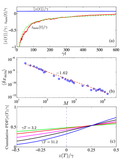
Figure 2: (a) The minimum of the finite time Lyapunov exponent over $M$ trajectories can remain negative, indicating converging trajectories, for very long times. It does converge to the mean Lyapunov exponent $\lambda=\langle z(t)\rangle$ (positive for a chaotic system), but the convergence described by (3) is very slow. The characteristic time of trajectory separation is $\gamma/\lambda\approx 15$. The exponent of the power law fit (dashed line) is $\alpha\approx 0.6$. (b) The smallest separation between $M$ initially uniformly distributed trajectories satisfied $\delta x_{\rm min}\sim M^{-\Gamma}$ with $\Gamma\approx 1.6$. (c) Cumulative probability for the value of the finite-time Lyapunov exponent, $z(t)$, at different values of the time (in dimensionless units). The distribution of $z(t)$ is very broad, even for large values of $t$. In all panels the parameters are the same as for Figure 1.

III Characterising the strong convergence of trajectories.

The finite-time Lyapunov exponent (FTLE) at time $t$ for a trajectory starting at $x_{0}$ is defined by Ott02

$$z(t)=\frac{1}{t}\ln\,\left|\frac{\partial x_{t}}{\partial x_{0}}\right|_{x(0)=x_{0}}\ ,$$ (2)

where $x_{t}$ denotes position at time $t$.

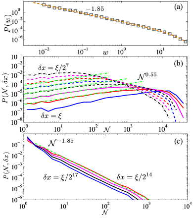
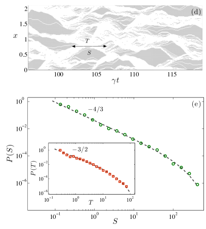
Figure 3: (a) The distribution of the numbers of particles in the trails is very broad, and is well approximated by a power-law in the small-mass limit. (b, c) Plots of the probability $P({\cal N},\delta x)$ for finding ${\cal N}$ particles in a cluster of size $\delta x$. There are power-law dependencies, with two different exponents characterising the sparse (b) and dense (c) regions. For this figure we used $\epsilon=1.75\epsilon_{\rm c}$. (d, e) Probability distributions of the areas $A$ and lifetimes $T$ of voids which are defined as the grey areas in panel (d).

If $z(t)$ is negative, this implies that nearby trajectories are converging towards each other. Figure 2(a) compares the minimum value of the FTLE over a sample of $M$ trajectories, denoted as $z_{\mathrm{min}}(t)$, with the average value of $z(t)$, termed the Lyapunov exponent $\lambda$. The crucial condition for chaos is that $\lambda$ is positive. However, in our simulations we find that the minimum value is negative up to a very long time, indicating that some trajectories show very long periods of convergence. In section V we argue that for a fixed number of particles $M\gg 1$, the minimal FTLE approaches $\lambda$ algebraically as $t\to\infty$ with

$$\lambda-z_{\rm min}(t)\sim\frac{f(M)}{\sqrt{t}},$$ (3)

where $f(M)$ is a function which increases monotonically (but slowly - approximately logarithmically) with $M$. Figure 2(a) shows the mean value of the minimum FTLE for (II), compared with a fit proportional to $t^{-\alpha}$, where $\alpha$ is a power close to $1/2$ (the parameters are the same as for Figure 1).

While the FTLE is negative, nearby trajectories are converging towards each other. Equation (3)) implies that the FTLE can be, in principle, made negative for arbitrarily long times by increasing the number of trajectories. This indicates that the closest approach of trajectories should decrease very rapidly as $M$ increases. This fact is illustrated in figure 2(b), where we show how the smallest separation $\delta x_{\rm min}$ between any trajectories of the flow illustrated in figure 1 decreases as the number of trajectories $M$ increases. Evaluating an ensemble average of $\delta x_{\rm min}$, we find a power-law behaviour, $\langle\delta x_{\rm min}\rangle\sim M^{-\Gamma}$, for $10<M<20000$ with $\Gamma\approx 1.6$.

Figures 2(a) and 2(b) present evidence that the most strongly converging trajectories lead to very high particle density. Figure 2(c) illustrates a complementary aspect of this phenomenon, by showing that converging regions occupy a large fraction of the phase space of our model. The cumulative PDF of $z$ is very broad: even at time $\gamma t=51.2$ (time has been made dimensionless by using the damping rate in (II)), the probability of $z$ being negative is as high as $\approx 1/3$.

IV Scale-free behaviour

Figure 1 shows evidence that the trajectories cluster into groups which we term ‘trails’. In figures 2(a) and 2(b) we showed evidence that there is an extremely broad distribution of density within these trails, including regions of extremely strong convergence. We also see evidence that the distribution of the numbers of trajectories in each trail is very broad, and characterised by a power-law. Figure 3(a) shows the probability distribution of the weights of trails for (II) for the parameters used in figure 1: we plotted the distribution of the number of trajectories inside an interval of length $\Delta x=L/4000$. We find that discrete models for particle trajectories, analogous to the Scheidegger river model Sch67 ; Hub91 , also show a similar power-law distribution of trail weights, indicating that this power-law is not a consequence of differential structure of the flow, and is therefore independent of properties of the FTLE.

We have described power laws which characterise the dense regions of figure 1. It is also of interest to understand the sparsely covered regions of this plot, and we find evidence that lacunarity of this image is also characterised by power laws. Let $P({\cal N},\delta x)$ be the probability that an interval of width $\delta x$ surrounding a given trajectory contains ${\cal N}$ other trajectories. In figures 3(b,c) we plot $P({\cal N},\delta x)$ versus ${\cal N}$, on doubly-logarithmic scales, for several values of $\delta x$. The plots suggest that when $\delta x\ll\xi$, $P({\cal N},\delta x)$ has a power-law dependence upon ${\cal N}$

$$P({\cal N},\delta x)\sim{\cal N}^{\beta}$$ (4)

with two different exponents, $\beta_{1}>0$ when ${\cal N}$ is below the position of the peak at ${\cal N}_{\rm max}$, and a different exponent $\beta_{2}<0$ above the peak. The exponents $\beta_{1}$ and $\beta_{2}$ depend upon $\epsilon$ (the coupling constant), but not upon $\delta x$ (interval width). We find that the exponent $\beta_{1}$ approaches zero as $\epsilon\to\epsilon_{\rm c}$: we used a larger value, $\epsilon=1.75\epsilon_{\rm c}$ in figures 3(b,c) so that $P({\cal N},\delta x)$ would show typical behaviour, with a clearly defined maximum.

As well as investigating the sparse regions of figure 1, we also investigated the PDF of the sizes of the voids, where there are no trajectories. Figures 3(d,e) show the definition of the area $A$ and lifetime $T$ of a void and how they are statistically distributed. Both plots show clear evidence for power laws at large values, with exponents $-4/3$ and $-3/2$ respectively (again, we used the same parameters as for figure 1). These exponents are readily explained by a model involving first passage processes.

It is well known that dynamical systems may have attractors with a fractal measure (often called strange attractors), thus leading to fractal clustering in phase space. This implies a power-law dependence of the mean number of trajectories $\langle{\cal N}\rangle$ in a ball of radius $\delta x$ surrounding a given trajectory: $\langle{\cal N}\rangle\sim\delta x^{D_{2}}$, where $D_{2}$ is a fractal dimension which is known as the correlation dimensionGra+83 . The power-laws which we have described, however, go beyond the fractal properties of strange attractors: whereas the fractal dimension describes the spatial structure of the most densely occupied regions, (4) describes the probability distribution of the amount of material in a region, rather than its spatial structure. In addition, the existence of more than one exponent demonstrates that our approach uncovers new properties of the system. Figures 2(b) and 3(b,c) indicate that the power-law distributions describe the sparsely occupied regions, as well as the dense regions. It is also interesting to note that the usual explanation for the fractal structure of the strange attractor, involving stretching and folding in phase space, is not applicable to this modelWil+12 .

V Theory for minimum FTLE

Here we present arguments which support equation (3). The arguments are most transparently presented for one-dimensional maps. They are also applicable to the continuous models in the main text, equations (II) and (VII.1), by considering the evolution over a finite time interval. For a one-dimensional map $x_{n+1}=F_{n}(x_{n})$, the finite-time Lyapunov exponent of a trajectory with initial position $x_{0}$ after $N$ iterations is

$$z(x_{0},N)=\frac{1}{N}\,\ln\,\left(\frac{\partial x_{N}}{\partial x_{0}}\right)\ .$$ (5)

If the trajectory reaches position $x_{j}(x_{0})$ after $j$ steps, starting from initial position $x_{0}$, then (using the chain rule) $z(x_{0},N)$ is a mean value of logarithms of gradients of the map along the trajectory:

$$z(x_{0},N)=\frac{1}{N}\sum_{j=1}^{N}\ln\,|F^{\prime}_{j}(x_{j}(x_{0}))|\ .$$ (6)

The Lyapunov exponent Ott02 is $\lambda=\lim_{N\to\infty}z(x_{0},N)$. We quantify the closest approaches of trajectories by considering the minimal value of the FTLE for a set of $M$ trajectories after $N$ iterations of the map. This will be denoted by $z_{\rm min}(N,M)$. For any fixed value of $M$, no matter how large, this quantity converges to $\lambda$ as $N\to\infty$.

The determination of $z_{\rm min}(N,M)$ is a problem which combines the large-deviation principal with extreme-value statistics. Because the dynamics is assumed to be chaotic, the FTLE (as expressed in equation (6)) may be regarded as a mean value of a sequence of random variables. The probability distribution of the FTLE can then be described by large deviation theory Fre+84 ; Tou09 , so that for large $N$ the probability density of $z$ has the asymptotic form

$$P(z)\sim\exp[-NJ(z)]$$ (7)

where $J(z)$ is a function which is termed a rate function or entropy function Fre+84 ; Tou09 . If we take a fixed number of trajectories and consider the long-time limit, $N\to\infty$, the $M$ different trajectories may be assumed to be drawn independently from a probability density in the large deviation theory form, equation (7). We are interested in the smallest value of $z$ for this sample of $M$ trajectories, $z_{\rm min}$. This problem in extreme-value statistics can be addressed by the method introduced by Gumbel Gum35 . In order to make a rough estimate of $z_{\rm min}(N,M)$, it is sufficient to find the value of $z$ for which the exponential smallness of the probability density balances the large number of samples, $M$, that is

$$MP(z_{\rm min})\sim 1\ .$$ (8)

In terms of the large deviation entropy function, this condition becomes: $M\,\exp[-NJ(z_{\rm min})]=1$. The logarithm of this equation gives the condition

$$\ln M-NJ(z_{\rm min})=0\ .$$ (9)

Now consider how equation (3) follows from equation (9). In the limit as $N\to\infty$, where $z_{\rm min}$ approaches $\lambda$, we are concerned with small values of $J(z)$, where the entropy can be approximated by a quadratic function:

$$J(z)=\frac{(z-\lambda)^{2}}{2\sigma^{2}}$$ (10)

indicating that equation (9) takes the form of equation (3), with $f(M)=\sigma\sqrt{2\ln M}$. However, when we made a careful numerical investigation of the distribution of $z_{\rm min}(N,M)$, we found that this expression does not give an accurate estimate for $f(M)$. In the following, we discuss our conclusions about the correct form for $f(M)$.

Firstly, we use the method introduced by Gumbel Gum35 to determine the probability density of the minimum value more precisely than (9). Namely, we find that the PDF of $z_{\rm min}$ is approximated by

$$\rho_{\rm min}(z)={\cal C}\,Z\,F(Y)$$ (11)

where ${\cal C}$ is a normalisation constant, and

$$Z=\frac{(\lambda-z)\sqrt{N}}{\sigma}\ ,\ \ \ Y=\frac{Z^{2}}{2}+\ln\left(\sqrt{2\pi}|Z|\right)-\ln\,M$$ (12)

with

$$F(Y)=\exp[-(Y+\exp(-Y))]\ .$$ (13)

Equations (11), (12) and (13) indicate that the typical size of $z_{\rm min}$ is of the form of equation (3), where the function $f(M)$ is actually a generalised Lambert function rather than a logarithm. A numerical integration indicates that the mean and variance of the minimum of the scaled variable $Z_{\rm min}$ are, respectively,

$$\langle Z_{\rm min}\rangle\approx\bar{Z}-\frac{0.41}{\sqrt{\ln\,M}}\ ,\ \ \ {\rm Var}(Z_{\rm min})\approx\frac{0.85}{\ln\,M}$$ (14)

where $\bar{Z}$ satisfies $Y(\bar{Z},M)=0$.

Now let us consider some numerical evidence on the applicability of the distribution defined by equations (11)-(13). In order to be able to make a thorough numerical study we examined a simplified version of the equation of motion (II), in the form of a map termed the correlated random walk Wil+12 :

$$x_{n+1}=x_{n}+f_{n}(x_{n})$$ (15)

where $f_{n}(x)$ are continuous and bounded random functions, drawn by independent sampling from an ensemble at each iteration. This map is a generalisation of a random walk, and can be used as a discrete model for advection of particles in a random flowWil+12 .

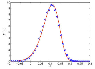
Figure 4: Probability distribution of the minimum FTLE for equation (15), for a sample of $M=1000$ trajectories after $N=200$ iterations, accumulating results using $2.5\times 10^{4}$ seeds of the random process in (V). This is compared with a fit to equations (11)-(13): the effective number of trajectories was $M_{\rm eff}=35.8$, and the variance $\sigma_{\rm eff}=1.2\sigma$.

Our numerical studies considered the case where $f_{n}(x)$ has a Gaussian distribution, with the following statistics:

$$\langle f_{n}(x)\rangle = 0$$

$$\langle f_{n}(x)f_{n^{\prime}}(x^{\prime})\rangle = \varepsilon^{2}\xi^{2}\,\exp\left[-\frac{(x-x^{\prime})^{2}}{2\xi^{2}}\right]\,\delta_{nn^{\prime}}\ .$$ (16)

We generated the $f_{n}(x)$ with approximately this correlation function by means of Fourier series, with period $L$ satisfying $\xi/L\ll 1$. The iterates $x_{n}$ are confined to the interval $[0,L]$ by adding an integer multiple of $L$ to $x_{n}$ every time a particle leaves the interval. This gives statistics which become stationary as $n\to\infty$. The quantities $\lambda$ and $\sigma$ are obtained from moments of the distribution of the gradient, $f^{\prime}(x)$, which has a Gaussian distribution with variance $\varepsilon^{2}$. It is known that the Lyapunov exponent of this model, $\lambda=\langle|1+f^{\prime}(x)|\rangle$, is positive for $\varepsilon>\varepsilon_{\rm c}$ with the critical point at $\varepsilon_{\rm c}=2.421\ldots$ Wil+12 . The numerical illustrations shown in figures 4 and 5, were for the case $\varepsilon=1.5\,\varepsilon_{\rm c}$, where $\lambda\approx 0.302$ and $\sigma\approx 1.107$.

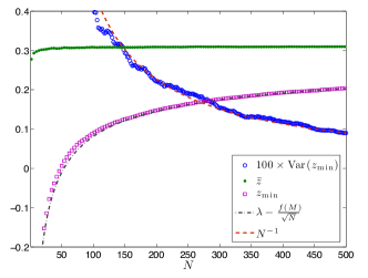
Figure 5: Average of the minimum value of the finite-time Lyapunov exponent over $10^{3}$ realisations of the random functions in the correlated random walk model, equations (15)-(V). The data are plotted as a function of the number of iterations, $N$, and compared with equation (3), where the used the fitting parameters $M_{\rm eff}=18.3$ and $\sigma_{\rm eff}=1.125\sigma$ in equations (14). We also show the variance of $z_{\rm min}$, compared with the fitted value.

We examined the probability distribution of $z_{\rm min}$, finding that it is of the form (11)-(13), with $M$ and $\sigma$ replaced by effective values, $M_{\rm eff}$ and $\sigma_{\rm eff}$. We find $\sigma_{\rm eff}/\sigma\approx 1$, and the difference is likely to be a consequence of the fact that $J(Z)$ is only approximately quadratic. However we find that $M_{\rm eff}/M\ll 1$. We interpret this as being a consequence of the clustering of trajectories illustrated in figure 1 of the main text. Because many of the trajectories are very closely clustered together, the number of independent samples of the phase space is much less than $M$. Figure 4 shows the probability distribution of $z_{\rm min}(N,M)$ for $M=10^{3}$ trajectories after $N=100$ iterations. There is an excellent fit to the distribution (11)-(13), with $\sigma_{\rm eff}=1.15\sigma$ and $M_{\rm eff}=35.8$.

We computed an ensemble average over different realisations of the random functions in equation (V). The ensemble averaged results are shown in figure 5, which shows the mean FTLE converging to $\lambda=0.302$, and the average of $z_{\rm min}(N,M)$ over $10^{3}$ realisations, for $M=100$ trajectories, compared to a fit of equation (3): there is excellent agreement with the prediction that $\lambda-\langle z_{\rm min}\rangle\sim N^{-1/2}$. We also computed the variance of $z_{\rm min}(N,M)$, which is asymptotic to a multiple of $N^{-1}$. Using the mean and the variance we were able to determine the two parameters $\sigma_{\rm eff}$ and $M_{\rm eff}$, obtaining $M_{\rm eff}=18.3$ and $\sigma_{\rm eff}=1.125\sigma$. This allowed us to fit the data to equations (14). We repeated this for different values of the number of trajectories, namely $M=100$, $10^{3}$ and $10^{4}$ trajectories, and we found fitted values of $\sigma_{\rm eff}/\sigma$ equal to $1.125$, $1.15$ and $1.175$ respectively. The fitted values of $M$ were $M_{\rm eff}=18.3$, $35.8$ and $75.5$ respectively. This is consistent with another power-law relation,

$$M_{\rm eff}=\mu M^{\Gamma}$$ (17)

with $\Gamma\approx 0.30$ for $\varepsilon=1.5\varepsilon_{\rm c}$.

VI Perpetually converging trajectories

In section V we emphasised the effects of the slow approach of $z_{\rm min}(N,M)$ towards $\lambda$ in the long-time limit, $N\to\infty$. For any given value of the number of iterations $N$ (or altenatively, for any time $t$), equation (3) indicates that $z_{\rm min}$ decreases as the number of trajectories $M$ increases. This raises the question as to what is the limit of $z_{\rm min}(N,M)$ as $M\to\infty$ for a fixed but large value of $N$. There will be a global minimum $\underline{z}(N)$ after $N$ iterations, which can be located by taking a sufficiently large number of initial conditions. Because of the exponential sensitivity of chaotic systems to their initial conditions, we expect that the number of trajectories, ${\cal M}$, required to accurately locate the global minimum of $z$ is ${\cal M}\sim K^{N}$, for some constant $K$. If we replace $M$ with ${\cal M}=K^{N}$ in equation (9), we obtain an equation $\ln\,K=J(z_{\rm min})$, which is independent of $N$. This suggests that the limit of $z$ as $M\to\infty$ should approach a limit $\mu$ as $N\to\infty$. This is not, however, a compelling argument because the derivation of (9) assumed that we take $M$ independent random samples of the distribution of $z$. If we increase $M$ so as to sample the entire phase-space, we cannot guarantee that the trajectories which yield extreme values are independent of each other.

However, there are arguments based upon exactly solvable systems which support the hypothesis that the global minimum of $z$ after $N$ iterations approaches a limit $\mu$ which is independent of $N$ and distinct from $\lambda$. Consider first a deterministic one-dimensional dynamical system for which it is obvious that $\mu<\lambda$. This is the generalised tent map

$$x_{n+1}=\left\{\begin{array}[]{lll}g_{1}x_{x}&,&0\leq x_{n}<g_{1}^{-1}\cr g_{2}(1-x_{n})&,&g_{1}^{-1}<x_{n}\leq 1\end{array}\right.\ .$$ (18)

The gradients of the linear sections, $g_{1}$ and $-g_{2}$ satisfy a harmonic mean value constraint: $g_{1}^{-1}+g_{2}^{-1}=1$. This is a piecewise linear map of the interval $[0,1]$ into itself. The Lyapunov exponent is

$$\lambda=\frac{g_{2}\,\ln\,g_{1}+g_{1}\,\ln\,g_{2}}{g_{1}+g_{2}}\ .$$ (19)

The $N$-fold composition of the map has $2^{N}$ piecewise linear intervals. If $g_{1}<g_{2}$, then the interval with the smallest FTLE is the first interval, for which the instability factor is $g_{1}^{N}$ and hence

$$\mu=\ln\,g_{1}$$ (20)

so that $\mu<\lambda$ if $g_{1}<g_{2}$. This elementary example shows that the minimal FTLE may converge to a value which is different from the Lyapunov exponent. The value of $\mu$ must, however, be positive for this map.

In order to see an example where $\mu$ may be negative while $\lambda$ is positive, implying that there is always at least one trajectory which is convergent for all times, we consider an alternative dynamical system. This system has two variables, $x_{N}$ and $y_{N}$, specifying the state at every iteration. The variables $y_{N}$ are iterated according to a simple tent map, representing a Bernoulli shift: $y_{N+1}=2y_{N}\,{\rm mod}\,1$. The iteration of the $x_{N}$ variable depends upon two random independent identically distributed random variables, $a_{n,\pm}$:

$$x_{n+1}=\left\{\begin{array}[]{lll}a_{n,+}\times x_{n}&,&0<y_{n}<\frac{1}{2}\cr a_{n,-}\times x_{n}&,&\frac{1}{2}<y_{n}<1\end{array}\right.\ .$$ (21)

We draw the $a_{n,\pm}$ independently from the same probability distribution. The initial condition for the $y_{N}$ variables is $y_{0}=x_{0}$. Consider the dynamics generated by this process as a map $x_{0}\rightarrow x_{N}$. The map is piecewise linear on a set of intervals, which are determined by the discontinuities of the process which generates the auxiliary variables $y_{N}$. After $N$ iterations there are $2^{N}$ such intervals. Within each interval, we have

$$x_{N}=\left[\prod_{j=1}^{N}a_{j,\pm}\right]x_{0}$$ (22)

where the $a_{j,\pm}$ are the random variables selected at random at each iteration, either $a_{j,+}$ or $a_{j,-}$ depending upon the trajectory $x_{j}$. These variables are chosen independently for each of the $2^{N}$ intervals. The FTLE for a given trajectory is, therefore,

$$z=\frac{1}{N}\sum_{j=1}^{N}\ln\,|a_{j,\pm}|$$ (23)

which is a mean value of a sum of random variables.

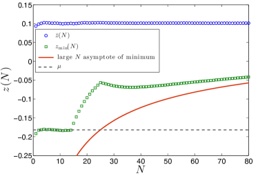
Figure 6: The ensemble average of the mean and minimum Lyapunov exponent for the map described by equations (21)-(23). Here $\sigma_{y}=0.5$, $\lambda=0.1$ and $M=2^{15}$, so that the ensemble average of the minimum of $z$ is equal to $\mu$ up until $N=14$. For large $N$ it approaches the asymptote given by equations (3) and (10)-(14), with $\sigma$ replaced by $\sigma_{y}/\sqrt{2}$. For this model, $M$ is not replaced by an effective value.

For the sake of definiteness, we make a simple and convenient choice for the statistics of the variables $a_{j,\pm}$. It is convenient to take the $a_{j,\pm}$ log-normally distributed, so that the probability distribution function of $y=\ln\,a$ is $P(y)=\exp[-(y-\lambda)^{2}/2\sigma_{y}^{2}]/\sqrt{2\pi}\sigma_{y}$, where $\lambda$ and $\sigma_{y}$ are two parameters. The variance of the sum is with respect to different choices of signs, but a fixed realisation of the $a_{j,\pm}$, is $\sigma_{y}^{2}/2$, so that $\sigma=\sigma_{y}/\sqrt{2}$ in equations (3), and (10)-(14). The ensemble average of the minimum value of $z$ over all choices of signs is equal to the average of the smaller of $a_{j,+}$ and $a_{j,-}$, which is approximately $-0.564\sigma_{y}$. The ensemble average of the minimum of $z$ is expected to equal

$$\mu\approx\lambda-0.564\sigma_{y}$$ (24)

until $2^{N}>M$, at which point the trajectories do not explore phase space in sufficient detail to identify the global minimum of $z$. These prediction were verified by a numerical experiment (see figure 6).

VII Applications

VII.1 Particle concentration in surface flows

We have used a one-dimensional model to illustrate our model, because it allows us to represent the space-time structures of the trajectories in a two-dimensional image such as Figure 1. There is, however, nothing in our discussion which is specific to one dimension, and the three-dimensional version of our model (II) is frequently used to describe the motion of particles in complex flows. It is already known that turbulent flows can induce fractal particle clusteringSom93 , although the effect is weaker than that illustrated in figure 1, because the underlying fluid flow is incompressible Bec07 (whereas our one-dimensional model, of necessity, involves a compressible flow). Clustering effects are believed to play a role in the production of raindrops in clouds Sun+97 ; Pum+16 (note however that other effects may be crucial to these processes Kos+05 ; Wil16 ).

The very strong convergence property, exhibited in Figure 1 is very reminiscent of the clustering of particles floating on the surface of a turbulent water tank Lar+09 . We remark that particles floating on the surface of a turbulent fluid experience a compressible and apparently random flow field. Experiments indicate that the correlation function of the particle distribution is $C(\Delta r)\sim\Delta r^{-0.92\pm 0.02}$ Lar+09 , implying that the particles cluster with a correlation dimension $D_{2}\approx 0.08$ Gra+83 . These observations show that surface flows are very close to a critical point at which path coalescence occurs. We modelled a surface flow by the equations of motion

$$\dot{\mbox{\boldmath$x$}} = \mbox{\boldmath$u$}(x,y,t),$$

$$u = \mbox{\boldmath$\nabla$}\wedge\psi+\alpha\mbox{\boldmath$\nabla$}\phi,$$ (25)

where $\psi(x,y,t)$ and $\phi(x,y,t)$ are two independent, isotropic, homogeneous scalar fields with a short correlation time, and $\alpha$ is an adjustable parameter. In this case it is known that $D_{2}=2(1-\alpha^{2})/(1+3\alpha^{2})$ Bal+01 , so that we can model the flow by taking $\alpha=0.926$. Figure 7 shows a simulation of this model for floating particles, where the particles become concentrated along lines of convergence associated with sinking fluid. Figure 7 is very reminiscent of experimental images Lar+09 , validating the use of this model.

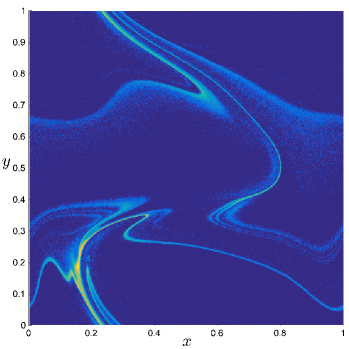
Figure 7: Simulation of the distribution of particles floating over a complex two-dimensional flow. ((VII.1) with $\alpha=0.926$.)

The investigation of  (VII.1) in two spatial dimensions reveals extreme convergence effects similar to those observed with the one-dimensional model (II). This is illustrated by Figure 7, which shows the positions of $10^{6}$ particles, which were originally evenly distributed in $10^{6}$ pixels. In Figure 7, one of the pixels has accumulated nearly $3\times 10^{4}$ particles. We have therefore provided evidence that, because surface flows are close to a critical point, they exhibit a pronounced form of the convergence phenomena displayed in Figure 1.

We propose that these effects, which combine strong convergence with mixing behaviour, may have played a role in the evolution of primitive living organisms. Early organisms would have lacked the mobility required to follow concentration gradients to find nutrients, to explore different environments, or to encounter other individuals which might have advantageous mutations. A process such as that illustrated in Figure 7, which combines mixing and converging behaviours, seems to offer advantages to primitive organisms. This supports the hypothesis that the first living organisms would have evolved in the surface layers of water, and that motion of the water could act as a catalyst for evolutionary development.

VII.2 Financial risks

The arguments that we have presented are quite general, indicating that the convergent chaos phenomenon, involving transient convergence of chaotic trajectories may find applications in very different domains. Insurance or futures transactions, where one takes a fee in exchange for writing a contract which requires a payment to be made if there is a loss or an unfavourable change in the price, may be an area ripe for the concept of convergent chaos. Substantial academic fields have developed around determining the value of these contracts. In insurance, actuarial methods are used Pro15 , and in finance, models based upon diffusive fluctuations of asset prices are the underlying tool Wil+95 . Any information about the nature of risk can be used to gain advantage. Our investigation shows that some chaotic systems, which would usually be assumed to be unpredictable, could be in fact highly predictable for certain initial conditions. Our results suggest that it may be possible to understand the conditions leading to a much smaller uncertainty than expected, so that the risk in a futures contract would be reduced.

VIII Discussion

Our results have shown that a simple chaotic dynamical system which describes the motion of particles in a turbulent flow can show an extremely high degree of convergence, despite the fact that the trajectories must eventually diverge with a positive rate of exponential growth. Using large-deviation and extreme-value concepts, we have shown that this transient convergence may be very long-lived, intense and widespread (as illustrated by our studies of the finite-time Lyapunov exponent), and that it exhibits several scale-free geometrical properties, revealed by exhibiting power-law distributions. The convergent chaos effect is expected to be observed in many systems, and we expect that it will be utilised for optimising the price of futures contracts. The model that we investigated in some depth, namely motion of particles in a turbulent flow, shows particularly marked convergence in the case of particles on the surface of a two-dimensional flow, and we argued that the combination of mixing and converging effects may have facilitated evolution of primitive organisms.

The phenomena described here have broad implications for the interpretation of chaos, specifically of the ‘butterfly effect’. Are perturbations destined to alter the course of large-scale patterns in turbulent systems? Or could regions of the phase space of a chaotic dynamical system be screened off from small perturbations? Our work clearly provides a positive answer to the latter question, thus bringing new insight on the Lorenz’ Brazilian butterfly problem. For these reasons the converging divergence phenomenon is likely to lead to a deeper understanding of chaotic dynamics and of its applications, and as such, deserves systematic investigation.

The authors are grateful to the Kavli Institute for Theoretical Physics for support, where this research was supported in part by the National Science Foundation under Grant No. PHY11-25915.

Author email addresses:

marc.pradas@open.ac.uk

alain.pumir@ens-lyon.fr

huber@kitp.ucsb.edu

m.wilkinson@open.ac.uk

References

- (1) E. Ott, Chaos in Dynamical Systems, 2nd edition, Cambridge: University Press, (2002).
- (2) E. N. Lorenz, in The Chaos Avant-Garde, eds. R. Abraham and Y. Ueda, World Scientific , Singapore, 2000).
- (3) E. N. Lorenz, in The Essence of Chaos, University College, London, (1995).
- (4) T. N. Palmer, A. Döring and G. Seregin, The real butterfly effect, Nonlinearity, 27, R123-R141, (2014).
- (5) H. Fujisaka, Statistical dynamics generated by fluctuations of local Lyapunov exponents, Prog. Theor. Phys., 70, 1264, (1983).
- (6) E. Aurell, G. Boffetta, A. Crisanti, G. Paladin, and A. Vulpiani, A., Growth of Non-infinitesimal Perturbations in Turbulence, Phys. Rev. Lett., 77, 1262, (1996).
- (7) S. H. Strogatz, Exploring complex networks, Nature, 410, 268-276, (2001).
- (8) K. D. Squire and J. K. Eaton, Preferential concentration of particles by turbulence, Phys. Fluids, A 3, 1169-1178, (1991).
- (9) G. Falkovich, K. Gawedzki and M. Vergassola, Particles and fields in turbulence, Rev. Mod. Phys., 73, 913-975, (2000).
- (10) R. Gatignol, Faxen formulae for a rigid particle in an unsteady non-uniform Stokes flow, J. Méc. Théor. Appl., 1, 143?60, (1983).
- (11) M. R. Maxey and J. J. Riley, Equation of motion for a small rigid sphere in a nonuniform flow, Phys. Fluids, 26, 883-9, (1983).
- (12) M. Wilkinson and B. Mehlig, The Path-Coalescence Transition and its Applications, Phys. Rev. E, 68, 040101, (2003).
- (13) M. I. Freidlin and A. D. Wentzell, Random Perturbations of Dynamical Systems, Grundlehren der Mathematischen Wissenschaften, vol. 260, Springer, New York, (1984).
- (14) H. Touchette, The large deviation approach to statistical mechanics, Phys. Rep. 478, 1 (2009).
- (15) E. J. Gumbel, Les valeurs extremes des distributions statistiques, Ann. Inst. Henri Poincaré, 5, 115-158, (1935).
- (16) A. E. Scheidegger, International Association of Scientific Hydrology Bulletin, 12, (1967).
- (17) G. Huber, Scheidegger’s rivers, Takayasu’s aggregates and continued fractions, Physica A, 170, 463-470, (1991).
- (18) P. Grassberger and I. Procaccia, Measuring the strangeness of strange attractors, Physica D, 9, 189-208, (1983).
- (19) M. Wilkinson, B. Mehlig, K. Gustavsson and E. Werner, Clustering of Exponentially Separating Trajectories, Eur. Phys. J. B, 85, 18, (2012).
- (20) J. C. Sommerer and E. Ott, Particles floating on a moving fluid - a dynamically comprehensible physical fractal, Science, 259, 335-39, (1993).
- (21) J. Bec, L. Biferale, M. Cencini, A. Lanotte, S. Musacchio, and F. Toschi, Heavy particle concentration in turbulence at dissipative and inertial scales, Phys. Rev. Lett., 98, 084502, (2007).
- (22) S. Sundaram and L. R. Collins, Collision statistics in an isotropic particle-laden turbulent suspension. Part 1. Direct numerical simulations J. Fluid Mech., 335, 75-109, (1997).
- (23) A. Pumir and M. Wilkinson, Collisional Aggregation due to Turbulence, Ann. Rev. Cond. Matter Phys., 7, 141-70, (2016).
- (24) A. B. Kostinski and R. A. Shaw, Fluctuations and luck in droplet growth by coalescence, Bull. Am. Met. Soc., 86, 235-244, (2005).
- (25) M. Wilkinson, Large Deviation Analysis of Rapid Onset of Rain Showers, Phys. Rev. Lett., 116, 018501, (2016).
- (26) J. Larkin, M. M. Bandi, A. Pumir and W. I. Goldburg, Power-law distributions of particle concentration in free-surface flows, Phys. Rev. E, 80, 066301,( 2009).
- (27) E. Balkovsky, G. Falkovich and A. Fouxon, Phys. Rev. Lett., 86, 2790, (2001).
- (28) S. D. Promislow, Fundamentals of Actuarial Mathematics, New York: Wiley, (2015).
- (29) P. Wilmott , S. Howison and J. Dewynne, The Mathematics of Financial Derivatives : A Student Introduction Cambridge: University Press, (1995).