Experimental protection of arbitrary states in a two-qubit subspace by nested Uhrig dynamical decoupling

Abstract

We experimentally demonstrate the efficacy of a three-layer nested Uhrig dynamical decoupling (NUDD) sequence to preserve arbitrary quantum states in a two-dimensional subspace of the four-dimensional two-qubit Hilbert space, on an NMR quantum information processor. The effect of the state preservation is studied first on four known states, including two product states and two maximally entangled Bell states. Next, to evaluate the preservation capacity of the NUDD scheme, we apply it to eight randomly generated states in the subspace. Although, the preservation of different states varies, the scheme on the average performs very well. The complete tomographs of the states at different time points are used to compute fidelity. State fidelities using NUDD protection are compared with those obtained without using any protection. The nested pulse schemes are complex in nature and require careful experimental implementation.

I Introduction

Dynamical decoupling (DD) sequences have found widespread application in quantum information processing (QIP), as strategies for protecting quantum states against decoherence Viola (2004). For a quantum system coupled to a bath, the DD sequence decouples the system and bath by adding a suitable decoupling interaction, periodic with cycle time $T_{c}$ to the overall system-bath Hamiltonian Viola et al. (1999). After $N$ applications of the cycle for a time $NT_{c}$, the system is governed by a stroboscopic evolution under an effective average Hamiltonian, in which system-bath interaction terms are no longer present.

The simplest DD sequences were motivated by early NMR spin-echo based schemes for coherent averaging of unwanted interactions Carr and Purcell (1954), and used periodic time-symmetrized trains of instantaneous $\pi$ pulses (equally spaced in time) to suppress decoherence. More sophisticated DD schemes are of the Uhrig dynamical decoupling (UDD) type, wherein the pulse timing in the DD sequence is tailored to produce higher-order cancellations in the Magnus expansion of the effective average Hamiltonian, thereby achieving system-bath decoupling to a higher order and hence stronger noise protection Uhrig (2008); Hodgson et al. (2010); Schroeder and Agarwal (2011); Yang et al. (2011); Liu et al. (2013). UDD schemes are applicable when the control pulses can be considered as ideal (i.e. instantaneous) and when the environment noise has a sharp frequency cutoff Dhar et al. (2006); Yang and Liu (2008); Uhrig (2009); Khodjasteh et al. (2011). These initial UDD schemes dealt with protecting a single qubit against different types of noise, and were later expanded to a whole host of optimized sequences involving nonlocal control operators, to protect multi-qubit systems against decoherence Mukhtar et al. (2010); Pan et al. (2011); Cong et al. (2011); Álvarez et al. (2012); West and Fong (2012); Ahmed et al. (2013). Quantum entanglement is considered to be a crucial resource for QIP, and several studies have explored the efficacy of UDD protocols in protecting such fragile quantum correlations against decay Agarwal (2010); Song et al. (2013); Franco et al. (2014). The experimental performance of UDD schemes have been demonstrated for trapped ion qubits undergoing dephasing Biercuk et al. (2009); Szwer et al. (2011), for electron spin qubits decohering in a spin bath Du et al. (2009) and for NMR qubits Álvarez et al. (2010); Ajoy et al. (2011); Roy et al. (2011). The freezing of state evolution using super-Zeno sequences was experimentally demonstrated using NMR Singh et al. (2014), and DD sequences were interleaved with quantum gate operations in an electron-spin qubit of a single nitrogen-vacancy center in diamond Zhang et al. (2014). Non-QIP applications of DD schemes include their usage for enhanced contrast in magnetic resonance imaging of tissue samples Jenista et al. (2009) and for suppression of NMR relaxation processes whilst studying molecular diffusion via pulsed field gradient experiments Álvarez et al. (2014).

While UDD schemes can well protect states against single- and two-axis noise (i.e. pure dephasing and/or pure bit-flip), they are not able to protect against general three-axis decoherence Kuo et al. (2012). Nested UDD (NUDD) schemes were hence proposed to protect multiqubit systems in generic quantum baths to arbitrary decoupling orders, by nesting several UDD layers and it was shown that the NUDD scheme can preserve a set of unitary Hermitian system operators (and hence all operators in the Lie algebra generated from this set of operators) that mutually either commute or anticommute Wang and Liu (2011). Furthermore, it was proved that the NUDD scheme is universal i.e. it can preserve the coherence of $m$ coupled qubits by suppressing decoherence upto order $N$, independent of the nature of the system-environment coupling Jiang and Imambekov (2011). Recently, a theoretical proposal examined in detail the efficiency of NUDD schemes in protecting unknown randomly generated two-qubit states and showed that such schemes are a powerful approach for protecting quantum states against decoherence Mukhtar et al. (2010).

This work focuses on the preservation of arbitrary states in a known two-dimensional subspace using appropriate NUDD sequences on an NMR quantum information processor. We first evaluate the efficacy of protection of the NUDD scheme by applying it on four specific states of the subspace ${\cal P}=\{|01\rangle,|10\rangle\}$ i.e. two separable states: $|01\rangle$ and $|10\rangle$, and two maximally entangled singlet and triplet Bell states: $\frac{1}{\sqrt{2}}(|01\rangle-|10\rangle)$ and $\frac{1}{\sqrt{2}}(|01\rangle+|01\rangle)$ in a four-dimensional two-qubit Hilbert space. Next, to evaluate the effectiveness of the NUDD scheme on the entire subspace, we randomly generate states in the subspace ${\cal P}$ (considered as a superposition of the known basis states $|01\rangle,|10\rangle$) and protect them using NUDD. We randomly generate eight states in the two-qubit subspace and protect them using a three-layer NUDD sequence. Full state tomography is used to compute the experimental density matrices. We allow each state to decohere, and compute the state fidelity at each time point without protection and after NUDD protection. The results are presented as a histogram and show that while NUDD is always able to provide some protection, the degree of protection varies from state to state.

This is the first experimental demonstration of the efficacy of NUDD sequences in protecting arbitrary states in a two-qubit subspace against arbitrary noise, upto a high-order. Although NUDD schemes are designed to be independent of any noise-model assumptions and also do not require a priori information about the state to be protected, they are experimentally challenging to implement as they involve repeating cycles of several dozen rf pulses. Nevertheless, their efficacy in suppressing decoherence to higher orders in multiqubit systems makes them promising candidates for realistic QIP. Our experiments are hence an important step forward in the protection of general quantum states against general decoherence.

This paper is organized as follows: Section II briefly recapitulates the NUDD scheme for two qubits and gives details of how the nesting of three layers of UDD is constructed in order to protect the diagonal populations and the off-diagonal coherences against decoherence. The explicit quantum circuit and corresponding NMR pulse sequences to implement NUDD on two qubits is given in Section III.1. The results of experimentally protecting four specific states in the known subspace are described in Section III.2. Section III.3 contains a detailed description of the NUDD protection of a randomly generated set of arbitrary states in the subspace of two NMR qubits. Finally, Section IV offers some concluding remarks.

II The NUDD scheme

Consider a two-qubit quantum system with its state space spanned by the states $\{|00\rangle,|01\rangle,|10\rangle,|11\rangle\}$, the eigenstates of the Pauli operator $\sigma_{z}^{1}\otimes\sigma_{z}^{2}$. Our interest is in protecting states in the subspace $\cal{P}$ spanned by states $\{|01\rangle,|10\rangle\}$, against decoherence. The density matrix corresponding to an arbitrary pure state $|\psi\rangle=\alpha|01\rangle+\beta|10\rangle$ belonging to the subspace $\cal{P}$ is given by

$$\rho(t)=\left(\begin{array}[]{cccc}0&0&0&0\\ 0&|\alpha|^{2}&\alpha\beta^{*}&0\\ 0&\beta\alpha^{*}&|\beta|^{2}&0\\ 0&0&0&0\end{array}\right)$$ (1)

with the coefficients $\alpha$ and $\beta$ satisfying $|\alpha|^{2}+|\beta|^{2}=1$ at time $t=0$. We briefly describe here the theoretical construction of a three-layer NUDD scheme to protect arbitrary states in the two-qubit subspace $\cal{P}$ Mukhtar et al. (2010, 2010).

The general total Hamiltonian of a two-qubit system interacting with an arbitrary bath can be written as

$$H_{\rm total}=H_{S}+H_{B}+H_{jB}+H_{12}$$ (2)

where $H_{S}$ is the system Hamiltonian, $H_{B}$ is the bath Hamiltonian, $H_{jB}$ is qubit-bath interaction Hamiltonian and $H_{12}$ is the qubit-qubit interaction Hamiltonian (which can be bath-dependent). Our interest here is in bath-dependent terms and their control, which can be expressed using a special basis set for the two-qubit system as follows Mukhtar et al. (2010, 2010):

$$H = H_{B}+H_{jB}+H_{12}$$

$$= H_{0}+H_{1}$$

$$H_{0} = \sum_{j=1}^{10}W_{j}Y_{j},\,\,H_{1}=\sum_{j=11}^{16}W_{j}Y_{j}$$ (3)

where the coefficients $W_{j}$ contain arbitrary bath operators. $Y$ are the special basis computed from the perspective of preserving the subspace spanned by the states $\{|01\rangle,|10\rangle\}$ in the two-qubit space Mukhtar et al. (2010, 2010):

$$Y_{1}=I,\quad\quad\quad\quad\,\,\,\,\,Y_{2}=|01\rangle\langle 01|+|10\rangle\langle 10|,$$

$$Y_{3}=|00\rangle\langle 11|,\quad\quad Y_{4}=|00\rangle\langle 00|-|11\rangle\langle 11|,$$

$$Y_{5}=|11\rangle\langle 00|,\quad\quad Y_{6}=|01\rangle\langle 01|-|10\rangle\langle 10|,$$

$$Y_{7}=|10\rangle\langle 00|,\quad\quad Y_{8}=|00\rangle\langle 10|,$$

$$Y_{9}=|10\rangle\langle 11|,\quad\quad Y_{10}=|11\rangle\langle 10|,$$

$$Y_{11}=|01\rangle\langle 00|,\quad\,\,\,\,Y_{12}=|00\rangle\langle 01|,$$

$$Y_{13}=|01\rangle\langle 11|,\quad\,\,\,\,Y_{14}=|11\rangle\langle 01|,$$

$$Y_{15}=|01\rangle\langle 10|+|10\rangle\langle 01|,$$

$$Y_{16}=-i(|10\rangle\langle 01|-|01\rangle\langle 10|).$$ (4)

The recipe to design UDD protection for a two-qubit state (say $|\chi\rangle$) is given in the following steps: (i) First a control operator $X_{c}$ is constructed using $X_{c}=I-2|\chi\rangle\langle\chi|$ such that $X_{c}^{2}=I$, with the commuting relation $[X_{c},H_{0}]=0$ and the anticommuting relation $\{X_{c},H_{1}\}=0$; (ii) The control UDD Hamiltonian is then applied so that system evolution is now under a UDD-reduced effective Hamiltonian thus achieving state protection upto order $N$; (iii) Depending on the explicit commuting or anticommuting relations of $X_{c}$ with $H_{0}$ and $H_{1}$, the UDD sequence efficiently removes a few operators $Y_{i}$ from the initial generating algebra of $H$ and hence suppresses all couplings between the state $|\chi\rangle$ and all other states.

To protect the general two-qubit state $|\psi\rangle$ in $\cal{P}$ against decoherence using NUDD, it has to be locked by nesting three layers of UDD sequences:

$\bullet$ Innermost UDD layer: The diagonal populations $\text{Tr}[\rho(t)|01\rangle\langle 01|]\approx|\alpha|^{2}$ are locked by this UDD layer with the control operator $X_{0}=I-2|01\rangle\langle 01|$. The reduced effective Hamiltonian is given by $H_{{\rm eff}}^{{\rm UDD-1}}=\sum_{i=1}^{10}D_{1,i}Y_{i}$, where $D_{1,i}$ refer to the expansion coefficients of this first UDD layer. Terms containing basis operators $Y_{11}\cdots Y_{16}$ are efficiently decoupled.

$\bullet$ Second UDD layer: The diagonal populations $\text{Tr}[\rho(t)|10\rangle\langle 10|]\approx|\beta|^{2}$ are locked by this second UDD layer with the control operator $X_{1}=I-2|10\rangle\langle 10|$. This UDD sequence is applied to the reduced effective Hamiltonian $H_{{\rm eff}}^{UDD-1}$ (defined in the step above), yielding a further reduced effective Hamiltonian $H_{{\rm eff}}^{UDD-2}=\sum_{i=1}^{6}D_{2,i}Y_{i}$ where $D_{2,i}$ refer to the expansion coefficients of this second UDD layer. Terms containing basis operators $Y_{7}\cdots Y_{10}$ are efficiently decoupled.

$\bullet$ Outermost UDD layer: The off-diagonal coherences $\text{Tr}[\rho(t)|01\rangle\langle 10|]\approx\alpha\beta^{*}$ are locked by this final UDD layer with the control operator $X_{\phi}=I-[|01\rangle+|10\rangle][\langle 01|+\langle 10|]$. The final reduced effective Hamiltonian after the three-layer NUDD contains five operators: $H_{{\rm eff}}^{{\rm UDD-3}}=\sum_{i=1}^{5}D_{3,i}Y_{i}$, where $D_{3,i}$ are the coefficients due to three UDD layers.

The innermost UDD control $X_{0}$ pulses are applied at the time intervals $T_{j,k,l}$, the middle layer UDD control $X_{1}$ pulses are applied at the time intervals $T_{j,k}$ and the outermost UDD control $X_{\phi}$ pulses are applied at the time intervals $T_{j}$ ($j,k,l=1,2,...N$) given by:

$$T_{j,k,l} = T_{j,k}+(T_{j,k+l}-T_{j,k})\sin^{2}{\left(\frac{l\pi}{2N+2}\right)}$$

$$T_{j,k} = T_{j}+(T_{j+1}-T_{j})\sin^{2}{\left(\frac{k\pi}{2N+2}\right)}$$

$$T_{j} = T\sin^{2}{\left(\frac{j\pi}{2N+2}\right)}$$ (5)

The total time interval in the $N^{th}$ order sequence is $(N+1)^{3}$ with the total number of pulses in one run being given by $N((N+1)^{2}+N+2)$ for even $N$ Mukhtar et al. (2010).

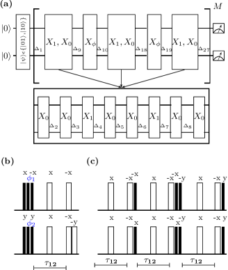
Figure 1: (Color online) (a) Circuit diagram for the three-layer NUDD sequence. The innermost UDD layer consists of $X_{0}$ control pulses, the middle layer comprises $X_{1}$ control pulses and the outermost layer consists of $X_{\phi}$ pulses. The entire NUDD sequence is repeated $M$ times; $\Delta_{i}$ are time intervals. (b) NMR pulse sequence to implement the control pulses for $X_{0}$ and $X_{1}$ UDD sequences. The values of the rf pulse phases $\phi_{1}$ and $\phi_{2}$ are set to $x$ and $y$ for the $X_{0}$ and to $-x$ and $-y$ for the $X_{1}$ UDD sequence, respectively. (c) NMR pulse sequence to implement the control pulses for the $X_{\phi}$ UDD sequence. The filled rectangles denote $\pi/2$ pulses while the unfilled rectangles denote $\pi$ pulses, respectively. The time period $\tau_{12}$ is set to the value $(2J_{12})^{-1}$, where $J_{12}$ denotes the strength of the scalar coupling between the two qubits.

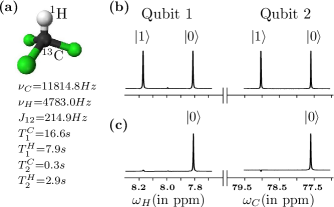
Figure 2: (Color online) (a) Structure of isotopically enriched chloroform-¹³C molecule, with the ¹H spin labeling the first qubit and the ¹³C spin labeling the second qubit. The system parameters are tabulated alongside with chemical shifts $\nu_{i}$ and scalar coupling $J_{12}$ (in Hz) and NMR spin-lattice and spin-spin relaxation times $T_{1}$ and $T_{2}$ (in seconds). (b) NMR spectrum obtained after a $\pi/2$ readout pulse on the thermal equilibrium state and (c) NMR spectrum of the pseudopure $|00\rangle$ state. The resonance lines of each qubit in the spectra are labeled by the corresponding logical states of the other qubit.

III Experimental protection of two qubits using NUDD

III.1 NMR implementation of NUDD

We now turn to the NUDD implementation for $N=2$ on a two-qubit NMR system. The entire NUDD sequence can be written in terms of UDD control operators $X_{0},X_{1},X_{\phi}$ (defined in the previous section) and time evolution $U(\delta_{i}t)$ under the general Hamiltonian for time interval fractions $\delta_{i}$:

$$X_{c}(t) = U(\delta_{1}t)X_{0}U(\delta_{2}t)X_{0}U(\delta_{3}t)X_{1}U(\delta_{4}t)X_{0}U(\delta_{5}t)X_{0}$$ (6)

$$U(\delta_{6}t)X_{1}U(\delta_{7}t)X_{0}U(\delta_{8}t)X_{0}U(\delta_{9}t)X_{\phi}U(\delta_{10}t)X_{0}$$

$$U(\delta_{11}t)X_{0}U(\delta_{12}t)X_{1}U(\delta_{13}t)X_{0}U(\delta_{14}t)X_{0}U(\delta_{15}t)$$

$$X_{1}U(\delta_{16}t)X_{0}U(\delta_{17}t)X_{0}U(\delta_{18}t)X_{\phi}U(\delta_{19}t)$$

$$X_{0}U(\delta_{20}t)X_{0}U(\delta_{21}t)X_{1}U(\delta_{22}t)X_{0}U(\delta_{23}t)$$

$$X_{0}U(\delta_{24}t)X_{1}U(\delta_{25}t)X_{0}U(\delta_{26}t)X_{0}U(\delta_{27}t)$$

In our implementation, the number of $X_{0},X_{1}$ and $X_{\phi}$ control pulses used in one run of the three-layer NUDD sequence are 18, 6 and 2, respectively.

Using the UDD timing intervals defined above and applying the condition $\sum\delta_{i}=1$, their values are computed to be

$$\{\delta_{i}\} = \{\beta,2\beta,\beta,2\beta,4\beta,2\beta,\beta,2\beta,\beta,2\beta,4\beta,2\beta,4\beta,8\beta,$$ (7)

$$4\beta,2\beta,4\beta,2\beta,\beta,2\beta,\beta,2\beta,4\beta,2\beta,\beta,2\beta,\beta\}$$

where the intervals between the $X_{0},X_{1}$ and $X_{\phi}$ control pulses turn out to be a multiple of $\beta=0.015625$ .

The NUDD scheme for state protection and the corresponding NMR pulse sequence is given in Fig. 1. The unitary gates $X_{0}$, $X_{1}$, and $X_{\phi}$ drawn in Fig. 1(a) correspond to the UDD control operators already defined in the previous section. The $\Delta_{i}$ time interval in the circuit given in Fig. 1(a) is defined by $\Delta_{i}=\delta_{i}t$, using the $\delta_{i}$ given in Eqn. (7). The pulses on the top line in Figs. 1(b) and (c) are applied on the first qubit (¹H spin in Fig. 2), while those at the bottom are applied on the second qubit (¹³C spin in Fig. 2), respectively. All the pulses are spin-selective pulses, with the $90^{\circ}$ pulse length being $7.6\mu$s and $15.6\mu$s for the proton and carbon rf channels, respectively. When applying pulses simultaneously on both the carbon and proton spins, care was taken to ensure that the pulses are centered properly and the delay between two pulses was measured from the center of the pulse duration time. We note here that the NUDD schemes are experimentally demanding to implement as they contain long repetitive cycles of rf pulses applied simultaneously on both qubits and the timings of the UDD control sequences were matched carefully with the duty cycle of the rf probe being used.

We chose the chloroform-¹³C molecule as the two-qubit system to implement the NUDD sequence (see Fig. 2 for details of system parameters and average NMR relaxation times of both the qubits). The two-qubit system Hamiltonian in the rotating frame (which includes the Hamiltonians $H_{S}$ and $H_{12}$ of Eqn. (2)) is given by

$$H_{\rm rot}=-(\nu_{H}I_{z}^{H}+\nu_{C}I_{z}^{C})+2\pi J_{12}I_{z}^{H}I_{z}^{C}$$ (8)

where $\nu_{H}$ ($\nu_{C}$) is the chemical shift of the ¹H(¹³C) spin, $I_{z}^{H}$($I_{z}^{C}$) is the $z$ component of the spin angular momentum operator for the ¹H(¹³C) spin, and $J_{12}$ is the spin-spin scalar coupling constant. The two qubits were initialized into the pseudopure state $|00\rangle$ using the spatial averaging technique Cory et al. (1998), with the corresponding density operator given by

$$\rho_{00}=\frac{1-\epsilon}{4}I+\epsilon|00\rangle\langle 00|$$ (9)

with a thermal polarization $\epsilon\approx 10^{-5}$ and $I$ being a $4\times 4$ identity operator. All experimental density matrices were reconstructed using a reduced tomographic protocol Leskowitz and Mueller (2004) and using the maximum likelihood estimation technique Singh et al. (2016). The fidelity of an experimental density matrix was computed by measuring the projection between the theoretically expected and experimentally measured states using the Uhlmann-Jozsa fidelity measure Uhlmann (1976); Jozsa (1994):

$$F=\left(Tr\left(\sqrt{\sqrt{\rho_{\rm theory}}\rho_{\rm expt}\sqrt{\rho_{\rm theory}}}\right)\right)^{2}$$ (10)

where $\rho_{\rm theory}$ and $\rho_{\rm expt}$ denote the theoretical and experimental density matrices respectively. The experimentally created pseudopure state $|00\rangle$ was tomographed with a fidelity of $0.99$.

Figure 3: Plot of fidelity versus time for (a) the $|01\rangle$ state and (b) the $|10\rangle)$ state, without any protection and after applying NUDD protection. The fidelity of both the states remains close to 1 for upto long times, after NUDD protection.

III.2 NUDD protection of known states in the subspace

We begin evaluating the efficiency of the NUDD scheme by first applying it to protect four known states in the two-dimensional subspace ${\cal P}$, namely two separable and two maximally entangled (Bell) states.

Protecting two-qubit separable states: We experimentally created the two-qubit separable states $|01\rangle$ and $|10\rangle$ from the initial state $|00\rangle$ by applying a $\pi_{x}$ on the second qubit and on the first qubit, respectively. The states were prepared with a fidelity of 0.98 and 0.97, respectively. One run of the NUDD sequence took 0.12756 s and $t=0.05$s (which included time taken to implement the control operators). The entire NUDD sequence was applied 40 times. The state fidelity was computed at different time instants, without any protection and after applying NUDD protection. The state fidelity remains close to 0.9 for long times (upto 5 seconds) when NUDD is applied, whereas for no protection the $|01\rangle$ state loses its fidelity (fidelity approaches 0.5) after 3 s and the $|10\rangle$ state loses its fidelity after 2 s. A plot of state fidelities versus time is displayed in Fig. 3, demonstrating the remarkable efficacy of the NUDD sequence in protecting separable two-qubit states against decoherence.

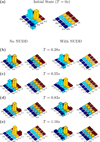
Figure 4: (Color online) Real (left) and imaginary (right) parts of the experimental tomographs of the (a) $\frac{1}{\sqrt{2}}(|01\rangle-|10\rangle)$ state, with a computed fidelity of 0.99. (b)-(e) depict the state at $T=0.28,0.55,0.83,1.10$s, with the tomographs on the left and the right representing the state without any protection and after applying NUDD protection, respectively. The rows and columns are labeled in the computational basis ordered from $|00\rangle$ to $|11\rangle$.

Figure 5: Plot of fidelity versus time for (a) the Bell singlet state and (b) the Bell triplet state, without any protection and after applying NUDD protection.

Protecting two-qubit Bell states: We next implemented NUDD protection on the maximally entangled singlet state $\frac{1}{\sqrt{2}}(|01\rangle-|10\rangle)$. We experimentally constructed the singlet state from the initial $|00\rangle$ state via the pulse sequence given in Fig. 6 with values of $\theta=-\frac{\pi}{2}$ and $\phi=0$. The fidelity of the experimentally constructed singlet state was computed to be 0.99. One run of the NUDD sequence took 0.27756 s and $t$ was kept at $t=0.2$s. The entire NUDD sequence was applied 4 times on the state. The singlet state fidelity at different time points was computed without any protection and after applying NUDD protection, and the state tomographs are displayed in Fig. 4 (tomographs for other states not shown). The fidelity of the singlet state remained close to 0.8 for 1 s when NUDD protection was applied, whereas when no protection is applied the state decoheres (fidelity approaches 0.5) after 0.55 s. We also implemented NUDD protection on the maximally entangled triplet state $\frac{1}{\sqrt{2}}(|01\rangle+|10\rangle)$. We experimentally constructed the triplet state from the initial $|00\rangle$ state via the pulse sequence given in Fig. 6 with values of $\theta=\frac{\pi}{2}$ and $\phi=0$. The fidelity of the experimentally constructed triplet state was computed to be 0.99. The total NUDD time was kept at $t=0.2$s and one run of the NUDD sequence took 0.27756 s. The entire NUDD sequence was repeated 4 times on the state. The state fidelity at different time points was computed without any protection and after applying NUDD protection. The fidelity of the triplet state remained close to 0.8 for 0.28 s when NUDD protection was applied, whereas when no protection is applied the state decoheres quite rapidly (fidelity approaches 0.5) after 0.28 s. A plot of state fidelities of both Bell states versus time is displayed in Fig. 5. While the NUDD scheme was able to protect the singlet state quite well (the time for which the state remains protected is double as compared to its natural decay time), it is not able to extend the lifetime of the triplet state to any appreciable extent. However, what is worth noting here is the fact that the state fidelity remains close to 0.8 under NUDD protection, implying that there is no “leakage” to other states.

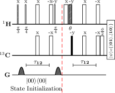
Figure 6: (Color online) NMR pulse sequence for the preparation of random states. The sequence of pulses before the vertical dashed red line achieve state initialization into the $|00\rangle$ state. The values of flip angles $\theta$ and $\phi$ of the rf pulses are randomly generated. Filled and unfilled rectangles represent $\frac{\pi}{2}$ and $\pi$ pulses respectively, while all other rf pulses are labeled with their respective flip angles and phases; the interval $\tau_{12}$ is set to $(2J_{12})^{-1}$ where $J_{12}$ is the scalar coupling.

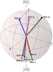
Figure 7: (Color online) Geometrical representation of eight randomly generated states on a Bloch sphere belonging to the two-qubit subspace ${\cal P}=\{|01\rangle,|10\rangle\}$. Each vector makes angles $\theta,\phi$ with the $z$ and $x$ axes, respectively. The state labels RS-$i$ ($i=1..8$) are explained in the text.

III.3 NUDD protection of unknown states in the subspace

We wanted to carry out an unbiased assessment of the efficacy of the NUDD scheme for state protection. To this end, we randomly generated several states in the two-dimensional subspace ${\cal P}$, and applied the NUDD sequence on each state.

Table 1: Results of applying NUDD protection on eight randomly generated states in the two-dimensional subspace. Each random state (RS) is tagged with a number for convenience, and its corresponding ($\theta$,$\phi$) angles are given in the column alongside. The fourth column displays the time at which the state fidelity approaches 0.5 (an estimate of the natural decay time of the state) and the last column displays the time for which state fidelity remains close to $\approx 0.8$ after applying NUDD protection.

State	Label	$(\theta,\phi)$(deg)	Decay Time (s)	Protected Time (s)
$0.2869|01\rangle+(0.9403+\iota 0.1828)|10\rangle$	RS-1	(147,57)	0.5s	1.0s
$0.1474|01\rangle-(0.7586+\iota 0.6346)|10\rangle$	RS-2	(163,349)	0.5s	1.1s
$0.9802|01\rangle+(0.1079-\iota 0.1662)|10\rangle$	RS-3	(23,345)	1.1s	1.1s
$0.1356|01\rangle+(0.3646-\iota 0.9212)|10\rangle$	RS-4	(164,175)	0.6s	1.1s
$0.9883|01\rangle+(0.1048+\iota 0.1109)|10\rangle$	RS-5	(18,51)	1.1s	1.1s
$0.9058|01\rangle+(0.2153+\iota 0.3648)|10\rangle$	RS-6	(50,152)	0.6s	0.9s
$0.0667|01\rangle+(-0.7693+\iota 0.6353)|10\rangle$	RS-7	(172,285)	0.6s	1.1s
$0.0551|01\rangle+(0.9861-\iota 0.1570)|10\rangle$	RS-8	(174,346)	0.6s	1.1s

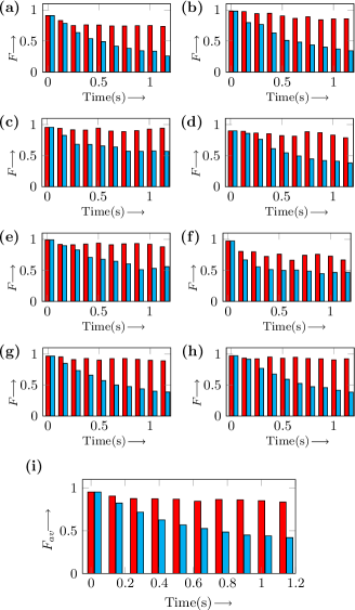
Figure 8: (Color online) Bar plots of fidelity versus time of eight randomly generated states (labeled RS-$i$, $i=1..8$), without any protection (blue bars) and after applying NUDD protection (red bars): (a) RS-1, (b) RS-2, (c) RS-3, (d) RS-4, (e) RS-5, (f) RS-6, (g) RS-7 and (h) RS-8. (i) Bar plot showing average fidelity of all eight randomly generated states, at each time point. The state labels are explained in the main text.

A general state in the two-qubit subspace ${\cal P}=\{|01\rangle,|10\rangle\}$ can be written in the form

$$|\psi\rangle=\cos{\frac{\theta}{2}}|01\rangle+e^{-\iota\phi}\sin{\frac{\theta}{2}}|10\rangle\$$ (11)

These states were experimentally created by using random values of $\theta$ and $\phi$ for the rf pulse flip angles, as detailed in Fig. 6. The eight randomly generated two-qubit states are shown in Fig. 7, where the distribution of the vectors on the Bloch sphere (corresponding to the two-dimensional subspace ${\cal P}$) shows that these states are indeed quite random. The entire three-layered NUDD sequence was applied 10 times on each of the eight random states. The time $t$ for the sequence was kept at $t=0.05$s and one run of the NUDD sequence took $0.12756$ s. The plots of fidelity versus time are shown as bar graphs in Fig. 8, with the blue bars representing state fidelity without any protection and the red bars representing state fidelity after NUDD protection. The final bar plot in Fig. 8(i) shows the average fidelity of all the randomly generated states at each time point. The results of protecting these random states via three-layered NUDD are tabulated in Table 1. Each state has been tagged by a label RS-$i$ (RS denoting “Random State” and $i=1,..8$), with its $\theta,\phi$ values displayed in the next column. The fourth column displays the values of the natural decoherence time (in seconds) of each state (estimated by computing the time at which state fidelity approaches 0.5). The last column in the table displays the time for which the state remains protected after applying NUDD (estimated by computing the time upto which state fidelity remains close to 0.8). While the NUDD scheme is able to protect specific states in the subspace with varying degrees of success (as evidenced from the entries in the last column of in Table 1), on an average as seen from the bar plot of the average fidelity in Fig. 8(i), the scheme performs quite well.

IV Conclusions

We experimentally implemented a three-layer nested UDD sequence on an NMR quantum information processor and explored its efficiency in protecting arbitrary states in a two-dimensional subspace of two qubits. The nested UDD layers were applied in a particular sequence and the full NUDD scheme was able to achieve second order decoupling of the system and bath. The scheme is sufficiently general as it does not assume prior information about the explicit form of the system-bath coupling. The experiments were highly demanding, with the control operations being complicated and involving manipulations of both qubits simultaneously. However, our results demonstrate that such systematic NUDD schemes can be experimentally implemented, and are able to protect multiqubit states in systems that are arbitrarily coupled to quantum baths.

The beauty of the NUDD schemes lies in the fact that one is sure the schemes will work to some extent! Furthermore, one need not know anything about the state to be protected or the nature of the quantum channel responsible for its decoherence. All one needs to know is the subspace to which the state belongs. Analogous to an expert huntswoman who knows her quarry well and sets her traps accordingly, if the QIP experimentalist has full knowledge of the state she wants to protect, she might be served better by using UDD schemes that are not nested. However if the nature of the beast to be captured is unclear, the QIP experimentalist might do better by setting a “generic trap” such as these NUDD schemes, knowing that some amount of state protection will always occur. Our study points the way to the realistic protection of fragile quantum states upto high orders and against arbitrary noise.