Emergence of a control parameter for the antiferromagnetic quantum critical metal

Abstract

We study the antiferromagnetic quantum critical metal in $3-\epsilon$ space dimensions by extending the earlier one-loop analysis [Sur and Lee, Phys. Rev. B 91, 125136 (2015)] to higher-loop orders. We show that the $\epsilon$-expansion is not organized by the standard loop expansion, and a two-loop graph becomes as important as one-loop graphs due to an infrared singularity caused by an emergent quasi-locality. This qualitatively changes the nature of the infrared (IR) fixed point, and the $\epsilon$-expansion is controlled only after the two-loop effect is taken into account. Furthermore, we show that a ratio between velocities emerges as a small parameter, which suppresses a large class of diagrams. We show that the critical exponents do not receive corrections beyond the linear order in $\epsilon$ in the limit that the ratio of velocities vanishes. The $\epsilon$-expansion gives critical exponents which are consistent with the exact solution obtained in $0<\epsilon\leq 1$.

I Introduction

Quantum critical points in metals host unconventional metallic states which lie outside the realm of Landau Fermi liquid theoryLandau (1957); Shankar (1994); Polchinski (1992). Experimentally, non-Fermi liquids are often characterized by anomalous dependencies of thermodynamic, spectroscopic and transport properties on temperature and energy Löhneysen et al. (2007); Stewart (2001). On the theoretical side, the quasiparticle paradigm based on well-defined single-particle excitations needs to be replaced with theories that capture strong interactions between soft collective modes and electronic excitations Holstein et al. (1973); Hertz (1976); Reizer (1989); Lee (1989); Lee and Nagaosa (1992); Millis (1993); Altshuler et al. (1994); Kim et al. (1994); Polchinski (1994); Nayak and Wilczek (1994); Senthil (2008); Lee (2009); Metlitski and Sachdev (2010a); Mross et al. (2010); Jiang et al. (2013); Fitzpatrick et al. (2013); Dalidovich and Lee (2013); Sur and Lee (2014); Holder and Metzner (2015); Schattner et al. (2016).

The antiferromagnetic (AF) quantum phase transition arises in a wide range of strongly correlated materials such as electron doped cupratesHelm et al. (2010), iron pnictidesHashimoto et al. (2012), and heavy fermion compoundsPark et al. (2006). Due to its relevance to many experimental systems, intensive analytical Abanov et al. (2003); Abanov and Chubukov (2000, 2004); Metlitski and Sachdev (2010b); Hartnoll et al. (2011); Abrahams and Wolfle (2012); de Carvalho and Freire (2013); Lee et al. (2013); Sur and Lee (2015); Maier and Strack (2016); Patel et al. (2015); Varma (2015) and numerical Berg et al. (2012); Schattner et al. (2015); Li et al. (2015); Gerlach et al. (2016); Wang et al. (2016); Li et al. (2016) efforts have been made to understand the nature of the non-Fermi liquid state. The AF quantum critical metal in two dimensions is described by a strongly interacting field theory for the AF spin fluctuations and electronic excitations near the Fermi surface. Although it seemed intractable, the theory for the $SU(2)$ symmetric AF quantum critical metal has been recently solved through a non-perturbative ansatzSchlief et al. (2016). The non-perturbative solution utilizes a ratio between velocities, which dynamically flows to zero at low energies, as a small parameter.

According to the non-perturbative solutionSchlief et al. (2016), the AF collective mode is strongly dressed by particle-hole excitations. In contrast, electrons have zero anomalous dimension, and exhibit a relatively weak departure from the Fermi liquid with dynamical critical exponent $z=1$. The non-perturbative solution actually applies to more general theories, and the same conclusion holds for the AF quantum critical point in the presence of a one-dimensional Fermi surface embedded in general dimensions, $2\leq d<3$Schlief et al. . However, the exact critical exponents obtained from the non-perturbative solution are not consistent with the earlier one-loop analysis of the theory in $3-\epsilon$ dimensions even in the small $\epsilon$ limitSur and Lee (2015). At the one-loop order, the ratio between velocities which is used as a small parameter in the non-perturbative solution does not flow to zero, and the electrons at the hot spots exhibit a stronger form of non-Fermi liquid with $z>1$.

In this work, we resolve this tension. We extend the earlier one-loop analysis to include higher-loop effects. We find that the $\epsilon$-expansion is not simply organized by the number of loops, and certain higher-loop diagrams are enhanced by IR singularities caused by an emergent quasi-locality. As a result, a two-loop diagram qualitatively modifies the nature of the fixed point even to the leading order in $\epsilon$Sur and Lee (2016). We show that the $\epsilon$-expansion is controlled with the inclusion of the two-loop effect. Furthermore, the ratio between velocities is shown to flow to zero in the low energy limit, which protects the critical exponents from receiving higher-loop corrections. This is similar to the nematic critical point in $d$-wave superconductors, where an emergent anisotropy in velocities leads to asymptotically exact results to all orders in the $1/N$ expansionHuh and Sachdev (2008).

The $\epsilon$-expansion and the non-perturbative solutionSchlief et al. (2016, ) are independent and complimentary. The former is a brute-force perturbative analysis, which is straightforward but valid only near the upper critical dimension. The latter approach is non-perturbative, and it is based on an Ansatz that is confirmed by a self-consistent computation. The agreement of the results from the two different approaches provides an independent justification of the Ansatz used in the non-perturbative solution.

II Model and dimensional regularization

We start with the theory for the AF quantum critical metal in two dimensions. We consider a Fermi surface with the $C_{4}$ symmetry. The low-energy degrees of freedom consist of the AF collective mode coupled to electrons near the hot spots, which are the set of points on the Fermi surface connected by the AF ordering vector Abanov and Chubukov (2000, 2004); Metlitski and Sachdev (2010b); Sur and Lee (2015), as is shown in Fig. 1. We study the minimal model, which has eight hot spots. The AF ordering is taken to be collinear with a commensurate wave vector. The action is written as

$$\mathcal{S}= \sum_{n=1}^{4}\sum_{m=\pm}\sum_{\sigma=\uparrow,\downarrow}\int\frac{d^{3}k}{(2\pi)^{3}}\leavevmode\nobreak\ {\psi}^{(m)*}_{n,\sigma}(k)\left[ik_{0}\leavevmode\nobreak\ +e^{m}_{n}(\vec{k};v)\right]\psi^{(m)}_{n,\sigma}(k)+\frac{1}{2}\int\frac{d^{3}q}{(2\pi)^{3}}\left[q_{0}^{2}+c^{2}|\vec{q}|^{2}\right]\vec{\phi}(-q)\cdot\vec{\phi}(q)$$ (1)

$$+g_{0}\sum_{n=1}^{4}\sum_{\sigma,\sigma^{\prime}=\uparrow,\downarrow}\int\frac{d^{3}k}{(2\pi)^{3}}\frac{d^{3}q}{(2\pi)^{3}}\leavevmode\nobreak\ \Bigl{[}\vec{\phi}(q)\cdot{\psi}^{(+)*}_{n,\sigma}(k+q)\vec{\tau}_{\sigma,\sigma^{\prime}}\psi^{(-)}_{n,\sigma^{\prime}}(k)+c.c.\Bigr{]}$$

$$+\frac{u_{0}}{4!}\int\frac{d^{3}k}{(2\pi)^{3}}\frac{d^{3}p}{(2\pi)^{3}}\frac{d^{3}q}{(2\pi)^{3}}\left[\vec{\phi}(k+q)\cdot\vec{\phi}(p-q)\right]\left[\vec{\phi}(-k)\cdot\vec{\phi}(-p)\right].$$

Here, $k=(k_{0},\vec{k})$ denotes the Matsubara frequency and the two-dimensional momentum $\vec{k}=(k_{x},k_{y})$. $\psi_{n,\sigma}^{(m)}$ are the fermion fields that carry spin $\sigma=\uparrow,\downarrow$ at the hot spots labeled by $n=1,2,3,4,\leavevmode\nobreak\ m=\pm$.

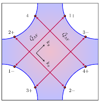
Figure 1: The first Brillouin zone of a metal in two dimensions with $C_{4}$ symmetry. The shaded region represents the occupied states. The AF ordering wavevector $\vec{Q}_{AF}$ is denoted by red arrows. The hot spots are the red dots connected by $\vec{Q}_{AF}$.

The choice of axis is such that the ordering wave vector is $\vec{Q}_{AF}=\pm\sqrt{2}\pi\hat{k}_{x},\pm\sqrt{2}\pi\hat{k}_{y}$ up to the reciprocal lattice vectors $\sqrt{2}\pi(\hat{k}_{x}\pm\hat{k}_{y})$. With this choice the fermion dispersions are $e^{\pm}_{1}(\vec{k};v)=-e^{\pm}_{3}(\vec{k};v)=vk_{x}\pm k_{y}$, $e^{\pm}_{2}(\vec{k};v)=-e^{\pm}_{4}(\vec{k};v)=\mp k_{x}+vk_{y}$, where $\vec{k}$ is the momentum deviation from each hot spot. The curvature of the Fermi surface can be ignored, since the patches of Fermi surface connected by the ordering vector are not parallel to each other with $v\neq 0$. The Fermi velocity along the ordering vector has been set to unity by rescaling $\vec{k}$. $v$ is the component of Fermi velocity that is perpendicular to $\vec{Q}_{AF}$. $\vec{\phi}(q)$ is the boson field with three components which describes the AF collective mode with frequency $q_{0}$ and momentum $\vec{Q}_{AF}+\vec{q}$. $\vec{\tau}$ represents the three generators of the $SU(2)$ group. $c$ is the velocity of the AF collective mode. $g_{0}$ is the Yukawa coupling between the collective mode and the electrons near the hot spots, and $u_{0}$ is the quartic coupling between the collective modes.

We generalize the theory by tuning the number of co-dimensions of the one-dimensional Fermi surfaceSenthil and Shankar (2009); Dalidovich and Lee (2013); Sur and Lee (2015). For this, we pair fermions on opposite sides of the Fermi surface into two component spinors, $\Psi_{1,\sigma}=(\psi_{1,\sigma}^{(+)},\psi_{3,\sigma}^{(+)})^{T}$, $\Psi_{2,\sigma}=(\psi_{2,\sigma}^{(+)},\psi_{4,\sigma}^{(+)})^{T}$, $\Psi_{3,\sigma}=(\psi_{1,\sigma}^{(-)},-\psi_{3,\sigma}^{(-)})^{T}$, $\Psi_{4,\sigma}=(\psi_{2,\sigma}^{(-)},-\psi_{4,\sigma}^{(-)})^{T}$. In the spinor basis, the kinetic term for the fermions becomes $S_{F}=\sum_{n=1}^{4}\sum_{\sigma=\uparrow,\downarrow}\int\frac{d^{3}k}{(2\pi)^{3}}\leavevmode\nobreak\ \bar{\Psi}_{n,\sigma}(k)\left[i\gamma_{0}k_{0}\leavevmode\nobreak\ +i\gamma_{1}\varepsilon_{n}(\vec{k};v)\right]\Psi_{n,\sigma}(k)$, where $\gamma_{0}=\sigma_{y}$ and $\gamma_{1}=\sigma_{x}$ ($\sigma_{i}$ being the Pauli matrices), $\bar{\Psi}_{n,\sigma}=\Psi^{\dagger}_{n,\sigma}\gamma_{0}$ with $\varepsilon_{1}(\vec{k};v)=e_{1}^{+}(\vec{k};v)$, $\varepsilon_{2}(\vec{k};v)=e_{2}^{+}(\vec{k};v)$, $\varepsilon_{3}(\vec{k};v)=e_{1}^{-}(\vec{k};v)$, $\varepsilon_{4}(\vec{k};v)=e_{2}^{-}(\vec{k};v)$. The general theory in $d$ spatial dimensions reads

$$\mathcal{S} =\sum_{n=1}^{4}\sum_{\sigma=1}^{N_{c}}\sum_{j=1}^{N_{f}}\int dk\leavevmode\nobreak\ \bar{\Psi}_{n,\sigma,j}(k)\Bigl{[}i\mathbf{\Gamma}\cdot\mathbf{K}+i\gamma_{d-1}\varepsilon_{n}(\vec{k};v)\Bigr{]}\Psi_{n,\sigma,j}(k)+\frac{1}{4}\int dq\leavevmode\nobreak\ \Bigl{[}\left|{\mathbf{Q}}\right|^{2}+c^{2}|\vec{q}|^{2}\Bigr{]}\mbox{Tr}\left[{\Phi(-q)\leavevmode\nobreak\ \Phi(q)}\right]$$ (2)

$$+i\frac{g\mu^{(3-d)/2}}{\sqrt{N_{f}}}\sum_{n=1}^{4}\sum_{\sigma,\sigma^{\prime}=1}^{N_{c}}\sum_{j=1}^{N_{f}}\int dkdq\leavevmode\nobreak\ \bar{\Psi}_{\bar{n},\sigma,j}(k+q)\Phi_{\sigma,\sigma^{\prime}}(q)\gamma_{d-1}\Psi_{n,\sigma^{\prime},j}(k)$$

$$+\frac{\mu^{3-d}}{4}\int dk_{1}dk_{2}dq\leavevmode\nobreak\ \Bigl{[}u_{1}\mbox{Tr}\left[{\Phi(k_{1}+q)\Phi(k_{2}-q)}\right]\mbox{Tr}\left[{\Phi(-k_{1})\Phi(-k_{2})}\right]+u_{2}\mbox{Tr}\left[{\Phi(k_{1}+q)\Phi(k_{2}-q)\Phi(-k_{1})\Phi(-k_{2})}\right]\Bigr{]}.$$

Here we consider $SU(N_{c})$ spin and $N_{f}$ flavors of fermions for generality. $k=(\mathbf{K},\vec{k})$ is the $(d+1)$-dimensional energy-momentum vector with $dk\equiv\frac{d^{d+1}k}{(2\pi)^{d+1}}$. $\vec{k}=(k_{x},k_{y})$ still denotes the two original momentum components, and $\mathbf{K}=(k_{0},k_{1},...,k_{d-2})$ denotes the frequency and the momentum components along the $(d-2)$ co-dimensions that have been added. $\mathbf{\Gamma}=(\gamma_{0},\gamma_{1},...,\gamma_{d-2})$ together with $\gamma_{d-1}$ are the gamma matrices which satisfy the Clifford algebra $\{\gamma_{\mu},\gamma_{\nu}\}=2I\delta_{\mu,\nu}$ with ${\rm Tr}[I]=2$. $\Psi_{n,\sigma,j}$ with $\sigma=1,2,...,N_{c}$ and $j=1,2,...,N_{f}$ is in the fundamental representation of both the enlarged spin group $SU(N_{c})$ and the flavor group $SU(N_{f})$. $\Phi(q)=\sum_{a=1}^{N_{c}^{2}-1}\phi^{a}(q)\tau^{a}$ is a matrix field for the collective mode, where $\tau^{a}$ are the generators of $SU(N_{c})$ with ${\rm Tr}[\tau^{a}\tau^{b}]=2\delta_{ab}$. The Yukawa interaction scatters fermions between pairs of hot spots denoted as $(n,\bar{n})$ with $\bar{1}=3$, $\bar{2}=4$, $\bar{3}=1$, $\bar{4}=2$. The Yukawa and quartic interactions have scaling dimensions $(3-d)/2$ and $(3-d)$, respectively, at the non-interacting fixed point. $\mu$ is the energy scale introduced to make $g,u_{1},u_{2}$ dimensionless. For $N_{c}\leq 3$, $u_{1}$ and $u_{2}$ are not independent couplings because of the identity, ${\rm Tr}[\Phi^{4}]=\frac{1}{2}({\rm Tr}[\Phi^{2}])^{2}$. The energy of the fermions is given by $E_{n}(k_{1},...,k_{d-2},\vec{k})=\pm\sqrt{\sum_{i=1}^{d-2}k_{i}^{2}+\varepsilon_{n}^{2}(\vec{k})}$, which supports a one-dimensional Fermi surface embedded in the $d$-dimensional momentum space. The theory respects the $U(1)\times SU(N_{c})\times SU(N_{f})$ internal symmetry. It is also invariant under the $C_{4}$ transformations in the $(k_{x},k_{y})$ plane, the $SO(d-1)$ that rotates $(k_{0},...,k_{d-2})$, and time-reversal. When $N_{c}=2$, there is an additional pseudospin symmetry, which rotates $\Psi_{n,\sigma,j}(k)$ into $i\tau_{\sigma,\sigma^{\prime}}^{(y)}\bar{\Psi}^{T}_{n,\sigma^{\prime},j}(-k)$Metlitski and Sachdev (2010b).

In three spatial dimensions the interactions are marginal. We therefore expand around $d=3$ using $\epsilon=3-d$ as a small parameter. We use the minimal subtraction scheme to compute the beta functions, which dictate the renormalization group (RG) flow of the velocities and couplings. To make the quantum effective action finite in the ultraviolet (UV), we add counter terms which can be written in the following form,

$$\mathcal{S}_{CT} = \sum_{n=1}^{4}\sum_{\sigma=1}^{N_{c}}\sum_{j=1}^{N_{f}}\int dk\leavevmode\nobreak\ \bar{\Psi}_{n,\sigma,j}(k)\left[i\mathcal{A}_{1}\mathbf{\Gamma}\cdot\mathbf{K}+i\mathcal{A}_{3}\gamma_{d-1}\varepsilon_{n}\left(\vec{k};\frac{\mathcal{A}_{2}}{\mathcal{A}_{3}}v\right)\right]\Psi_{n,\sigma,j}(k)$$ (3)

$$+\frac{1}{4}\int dq\leavevmode\nobreak\ \Bigl{[}\mathcal{A}_{4}\left|{\mathbf{Q}}\right|^{2}+\mathcal{A}_{5}\leavevmode\nobreak\ c^{2}\left|{\vec{q}}\right|^{2}\Bigr{]}\mbox{Tr}\left[{\Phi(-q)\leavevmode\nobreak\ \Phi(q)}\right]$$

$$+i\mathcal{A}_{6}\frac{g\mu^{(3-d)/2}}{\sqrt{N_{f}}}\sum_{n=1}^{4}\sum_{\sigma,\sigma^{\prime}=1}^{N_{c}}\sum_{j=1}^{N_{f}}\int dk\,dq\leavevmode\nobreak\ \Bigl{[}\bar{\Psi}_{\bar{n},\sigma,j}(k+q)\Phi_{\sigma,\sigma^{\prime}}(q)\gamma_{d-1}\Psi_{n,\sigma^{\prime},j}(k)\Bigr{]}$$

$$+\frac{\mu^{3-d}}{4}\int dk_{1}\,dk_{2}\,dq\leavevmode\nobreak\ \Bigl{[}\mathcal{A}_{7}u_{1}\mbox{Tr}\left[{\Phi(k_{1}+q)\Phi(k_{2}-q)}\right]\mbox{Tr}\left[{\Phi(-k_{1})\Phi(-k_{2})}\right]$$

$$+\mathcal{A}_{8}u_{2}\mbox{Tr}\left[{\Phi(k_{1}+q)\Phi(k_{2}-q)\Phi(-k_{1})\Phi(-k_{2})}\right]\Bigl{]},$$

where

$$\mathcal{A}_{n}\equiv\mathcal{A}_{n}(v,c,g,u;\epsilon)=\sum_{m=1}^{\infty}\frac{Z_{n,m}(v,c,g,u)}{\epsilon^{m}}.$$ (4)

$Z_{n,m}(v,c,g,u)$ are finite functions of the couplings. The counter terms are computed order by order in $\epsilon$. The general expressions for the dynamical critical exponent, the anomalous scaling dimensions of the fields, and the beta functions of the velocities and couplings are summarized in Section III. More details on the RG procedure can be found in Ref. Sur and Lee (2015).

III The modified one-loop fixed point

Figure 2: One-loop diagrams.

We begin by reviewing the one-loop RG analysis of Ref. Sur and Lee (2015). The conclusion of the analysis is that the theory flows to a quasi-local non-Fermi liquid state, where $c,v$ flow to zero as $1/l$ for $d<3$ and as $1/\log(l)$ at $d=3$ in the logarithmic length scale $l$, with their ratio fixed to be $w\equiv v/c=\frac{N_{c}N_{f}}{N_{c}^{2}-1}$ in the low energy limit with $l\rightarrow\infty$. Along with the emergent quasi-locality, the couplings also flow to zero such that $\lambda\equiv g^{2}/v$ and $\kappa_{i}\equiv u_{i}/c^{2}$ flow to $\lambda^{*}=\frac{4\pi(N_{c}^{2}+N_{c}N_{f}-1)}{N_{c}^{2}+N_{c}N_{f}-3}\epsilon$ and $\kappa_{i}^{*}=0$ in the low energy limit.

The perturbative expansion is controlled by the ratios between the couplings and the velocities, and the dynamical critical exponent becomes $z=1+\frac{N_{c}^{2}+N_{c}N_{f}-1}{2(N_{c}^{2}+N_{c}N_{f}-3)}\epsilon$. With $w\sim\mathcal{O}(1)$ at the one-loop fixed point, general diagrams are estimated to scale as $I\sim\lambda^{\frac{V_{g}}{2}}\kappa_{i}^{V_{u}}c^{V_{u}-L_{b}+\frac{E-2}{2}}$, where $V_{g}$ is the number of Yukawa vertices, $V_{u}$ is the number of quartic vertices, $L_{b}$ is the number of boson loops, and $E$ is the number of external lines. Because $c$ flows to zero, magnitudes of higher-loop quantum corrections are controlled not only by $\lambda$ but also by $c$. In particular, the quantum correction to the spatial part of the boson kinetic term becomes $\mathcal{A}_{5}\sim I/c^{2}\sim\lambda^{\frac{V_{g}}{2}}\leavevmode\nobreak\ \kappa_{i}^{V_{u}}\leavevmode\nobreak\ c^{V_{u}-L_{b}-2}$, where the counter term is further enhanced by a factor of $1/c^{2}$ because the velocity in the classical action is already small.

In three dimensions ($\epsilon=0$), all higher-loop diagrams are suppressed because $\lambda$ flows to zero faster ($\lambda\sim 1/l$) than the velocities ($v\sim c\sim 1/\log(l)$). Therefore, the critical point in three dimensions is described by the stable quasi-local marginal Fermi liquid Varma et al. (1989), where the Fermi liquid is broken by logarithmic corrections from the one-loop effectSur and Lee (2015). Below three dimensions ($\epsilon>0$), however, some higher-loop diagrams cannot be ignored because $c$ flows to zero while $\lambda^{*}\sim\epsilon$. For example, $\mathcal{A}_{5}$ from Fig. 3 is divergent at the one-loop fixed point. It might seem strange that the higher-loop graph suddenly becomes important for any nonzero $\epsilon$ while it is negligible at $\epsilon=0$. This apparent discontinuity originates from the fact that the small $\epsilon$ limit and the low energy limit do not commute. If the small $\epsilon$ limit is taken first, all higher-loop graphs are suppressed. However, since we are ultimately interested in the theory at $d=2$, we fix $\epsilon$ to a small but finite value, and then take the low energy limit of the corresponding theory. In this case, $c$ flows to zero, and the IR singularity caused by the softening of the collective mode enhances the magnitude of the two-loop graph. Since certain higher-loop diagrams can be enhanced by the IR singularity in the small $c$ limit, we cannot ignore all higher-order quantum corrections from the outset even in the small $\epsilon$ limit.

The largest contribution to the renormalization of $c$ comes from the boson self-energy in Fig. 3. We call the addition of this two-loop diagram to the one-loop diagrams (Fig. 2) the “modified-one-loop” (M1L) order. As will be shown later, the flow of $c$ is modified by the two-loop graph in Fig. 3 such that the effect of other higher-loop diagrams is negligible in the small $\epsilon$ limit. There also exists a two-loop diagram made of quartic vertices contributing to $\mathcal{A}_{5}$. However, the diagram has no enhancement by $1/c^{2}$ because the momentum dependent self-energy comes with $c^{2}$ due to the $(d+1)$-dimensional rotational symmetry present in the bosonic sector. The contribution from the quartic vertices are further suppressed because $\kappa_{i}$ is irrelevant at the fixed point.

Figure 3: Two-loop diagram for the boson self-energy.

Fig. 3 gives rise to the quantum effective action whose divergent part is given by

$$\delta\Gamma_{0,2}^{2L}=\frac{1}{\epsilon}\frac{4}{N_{c}N_{f}}\frac{g^{4}}{v^{2}c^{2}}h_{5}(v,c)\int dp\leavevmode\nobreak\ \frac{1}{4}c^{2}|\vec{p}|^{2}\text{Tr}[\Phi(-p)\Phi(p)],$$ (5)

where $h_{5}(v,c)$ is given by $h_{5}(v,c)=h_{5}^{*}\frac{v}{c}$ with $h_{5}^{*}\approx 5.7\times 10^{-4}$ in the limit $v,c,v/c$ are small. The full definition of $h_{5}(v,c)$ is given in Appendix B. The positive sign of Eq. (5) implies that the two-loop correction prevents $c$ from flowing to zero too fastSur and Lee (2016). If $c$ is small, the quantum correction makes the collective mode speed up until the quantum correction becomes $\mathcal{O}(1)$, $\frac{1}{\epsilon}\frac{4}{N_{c}N_{f}}\frac{g^{4}}{v^{2}c^{2}}h_{5}(v,c)\sim 1$. Since $\frac{g^{2}}{v}\sim\epsilon$, this suggests that $\frac{g^{2}}{c^{3}}$ becomes $\mathcal{O}(1)$ in the low energy limit. Once $c$ becomes comparable to $g^{2/3}\sim v^{1/3}$, it flows to zero together with $v$, although at a slower rate than $v$. As a result, $w=v/c$ flows to zero at the M1L fixed point for $\epsilon>0$, unlike at $\epsilon=0$. This emergent hierarchy in the velocities plays a crucial role in the non-perturbative solutionSchlief et al. (2016, ). In order to confirm this picture, we examine the RG flow in the space of $\{\lambda,x,w,\kappa_{i}\}$, where $x\equiv\frac{g^{2}}{c^{3}}$ is expected to flow to an $\mathcal{O}(1)$ value at the fixed point.

The beta functions for the five parameters are expressed in terms of the counter terms as

$$\frac{d\lambda}{dl} = z\leavevmode\nobreak\ \lambda\left(\epsilon+Z_{2,1}^{\prime}+Z_{3,1}^{\prime}+Z_{4,1}^{\prime}-2Z_{6,1}^{\prime}\right),$$

$$\frac{dx}{dl} = z\leavevmode\nobreak\ x\left(\epsilon+\frac{1}{2}\left(6Z_{1,1}^{\prime}-2Z_{3,1}^{\prime}-Z_{4,1}^{\prime}+3Z_{5,1}^{\prime}-4Z_{6,1}^{\prime}\right)\right),$$

$$\frac{dw}{dl} = \frac{1}{2}\leavevmode\nobreak\ z\leavevmode\nobreak\ w\left(2Z_{1,1}^{\prime}-2Z_{2,1}^{\prime}-Z_{4,1}^{\prime}+Z_{5,1}^{\prime}\right),$$

$$\frac{d\kappa_{1}}{dl} = z\leavevmode\nobreak\ \kappa_{1}\left(\epsilon+Z_{4,1}^{\prime}+Z_{5,1}^{\prime}-Z_{7,1}^{\prime}\right),$$

$$\frac{d\kappa_{2}}{dl} = z\leavevmode\nobreak\ \kappa_{2}\left(\epsilon+Z_{4,1}^{\prime}+Z_{5,1}^{\prime}-Z_{8,1}^{\prime}\right),$$ (6)

where $Z_{n,1}^{\prime}\equiv\left(\frac{1}{2}g\partial_{g}+u_{i}\partial_{u_{i}}\right)Z_{n,1}$, and $z=\left[1+Z_{1,1}^{\prime}-Z_{3,1}^{\prime}\right]^{-1}$ is the dynamical critical exponent. In the limit that $v,c,v/c$ are small, the beta functions at the M1L level become

$$\frac{d\lambda}{dl} = z\leavevmode\nobreak\ \lambda\Bigg{(}\epsilon-\frac{1}{4\pi}\lambda+\frac{1}{2\pi N_{c}N_{f}}\leavevmode\nobreak\ \lambda w\Bigg{)},$$ (7)

$$\frac{dx}{dl} = z\leavevmode\nobreak\ x\leavevmode\nobreak\ \Bigg{(}\epsilon-\frac{3N_{c}^{2}-7}{8\pi N_{c}N_{f}}\leavevmode\nobreak\ \lambda w+\frac{(N_{c}^{2}-1)}{2\pi^{2}N_{c}N_{f}}\leavevmode\nobreak\ \frac{(\lambda w)^{\frac{3}{2}}}{x^{\frac{1}{2}}}+\frac{1}{8\pi}\lambda-\frac{12\,h_{5}^{*}}{N_{c}N_{f}}\leavevmode\nobreak\ \lambda\,x\Bigg{)},$$ (8)

$$\frac{dw}{dl} = \frac{1}{2}\leavevmode\nobreak\ z\leavevmode\nobreak\ w\Bigg{(}-\frac{(N_{c}^{2}-1)}{4\pi N_{c}N_{f}}\leavevmode\nobreak\ \lambda w-\frac{(N_{c}^{2}-1)}{\pi^{2}N_{c}N_{f}}\leavevmode\nobreak\ \frac{(\lambda w)^{\frac{3}{2}}}{x^{\frac{1}{2}}}+\frac{1}{4\pi}\lambda-\frac{8\,h_{5}^{*}}{N_{c}N_{f}}\leavevmode\nobreak\ \lambda\,x\Bigg{)},$$ (9)

$$\frac{d\kappa_{1}}{dl} = z\leavevmode\nobreak\ \kappa_{1}\left(\epsilon-\frac{1}{4\pi}\lambda-\frac{8\,h_{5}^{*}}{N_{c}N_{f}}\leavevmode\nobreak\ \lambda\,x-\frac{1}{2\pi^{2}}\left((N_{c}^{2}+7)\kappa_{1}+2\left(2N_{c}-\frac{3}{N_{c}}\right)\kappa_{2}+3\left(1+\frac{3}{N_{c}^{2}}\right)\frac{\kappa_{2}^{2}}{\kappa_{1}}\right)\right),$$ (10)

$$\frac{d\kappa_{2}}{dl} = z\leavevmode\nobreak\ \kappa_{2}\left(\epsilon-\frac{1}{4\pi}\lambda-\frac{8\,h_{5}^{*}}{N_{c}N_{f}}\leavevmode\nobreak\ \lambda\,x-\frac{1}{2\pi^{2}}\left(12\kappa_{1}+2\left(N_{c}-\frac{9}{N_{c}}\right)\kappa_{2}\right)\right),$$ (11)

with $z=\left(1-\frac{N_{c}^{2}-1}{8\pi N_{c}N_{f}}\lambda w\right)^{-1}$. The beta functions exhibit a stable fixed point given by

$$\lambda^{*}=4\pi\epsilon,\quad x^{*}=\frac{N_{c}N_{f}}{32\pi\,h_{5}^{*}},\quad w^{*}=0,\quad\kappa_{i}^{*}=0.$$ (12)

It is noted that $x$ is $\mathcal{O}(1)$, and $v,c,v/c$ all vanish at the fixed point.

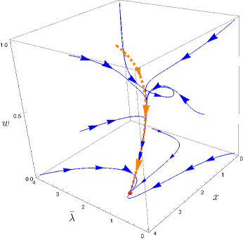
Figure 4: The RG flow in the space of $(\lambda,x,w)$ for $\epsilon=0.01$ and $N_{c}=2,N_{f}=1$. The axes are scaled as $\bar{x}\equiv x/10$, $\bar{\lambda}\equiv 10\lambda$. The fixed point $(\bar{\lambda}^{*},\bar{x}^{*},w^{*})=(1.26,3.49,0)$ is denoted as a red dot. The solid curves represent the numerically integrated RG flows, and the dotted (orange) line represents the one-dimensional manifold given by $\frac{dx}{dl}=\frac{d\lambda}{dl}=0$.

In order to understand the flow near the fixed point, we first examine the beta functions for $x$ and $\lambda$. Although it may seem arbitrary to focus on the flow of $x,\lambda$ first with fixed $w$, this is actually a good description of the full RG flow because the flow of $x,\lambda$ is much faster than that of $w$, as will be shown in the following. From Eqs. (7), (8), the beta functions for $(\delta\lambda,\delta x)\equiv(\lambda-\lambda^{*},x-x^{*})$ are given by

$$\frac{d\delta\lambda}{dl} = f_{\lambda}(w)-\epsilon\leavevmode\nobreak\ \delta\lambda+\dots,$$

$$\frac{d\delta x}{dl} = f_{x}(w)-\frac{N_{c}N_{f}}{32\pi\,h_{5}^{*}}\,\Bigg{(}\frac{48\pi\,h_{5}^{*}\epsilon\delta x}{N_{c}N_{f}}+\frac{\delta\lambda}{4\pi}\Bigg{)}+\dots$$

to the linear order in the deviation from the fixed point for small $w$, where $f_{\lambda}(w)=\left.\frac{d\lambda}{dl}\right|_{\lambda=\lambda^{*},x=x^{*}}$, $f_{x}(w)=\left.\frac{dx}{dl}\right|_{\lambda=\lambda^{*},x=x^{*}}$, and $\dots$ represent terms that are higher order in $\delta\lambda$, $\delta x$. Eq. (LABEL:eq:x_beta_function_lowest_order) implies that the perturbations in $\lambda$ and $x$ are irrelevant at the fixed point, and they flow to $w$-dependent values exponentially in $l$. This can be seen from Fig. 4, which shows the full numerical solution to the beta functions for $(\lambda,x,w)$. Once the RG flow reaches the one-dimensional manifold given by $(\lambda,x,w)=\left(\lambda^{*}+\frac{f_{\lambda}(w)}{\epsilon},x^{*}+\frac{2}{3\epsilon}\left[f_{x}(w)-\frac{N_{c}N_{f}f_{\lambda}(w)}{128\pi^{2}\,h_{5}^{*}\epsilon}\right],w\right)$, $w$ flows to the fixed point at a slower rate. To compute the flow within this manifold, we set $\frac{d\lambda}{dl}=\frac{dx}{dl}=0$ in Eq. (6) to express $Z_{1,1}$, $Z_{4,1}$ in terms of $Z_{n,1}$ with $n=2,3,5,6$. This gives the beta function for $w$ within the manifold,

$$\frac{dw}{dl} = \frac{2z}{3}\left(-Z_{2,1}^{{}^{\prime}}+Z_{3,1}^{{}^{\prime}}\right)w,$$ (14)

which reduces to

$$\frac{dw}{dl}=-\frac{64\sqrt{2h_{5}^{*}}(N_{c}^{2}-1)}{3(N_{c}N_{f})^{3/2}}\epsilon^{3/2}\,w^{5/2}$$ (15)

to the leading order in $w$. Because the flow velocity of $w$ vanishes to the linear order in $w$, $w$ flows to zero as a power-law in the logarithmic length scale, $w\sim l^{-2/3}$. At the fixed point, the quartic couplings are irrelevant and their beta functions become

$$\frac{d\kappa_{i}}{dl} = -\epsilon\kappa_{i},$$ (16)

to the leading order in $w$ and $\kappa_{i}$. This confirms that the fixed point in Eq. (12) is stable.

In the small $\epsilon$ limit, Eq. (12) does not converge to the one-loop fixed point, $\lambda^{*}=0$, $x^{*}=0$, $w^{*}=\frac{N_{c}N_{f}}{N_{c}^{2}-1}$, $\kappa_{i}^{*}=0$, which represents the correct fixed point at $\epsilon=0$. Although the beta functions are analytic functions of $\epsilon$, the fixed point is not because the low energy limit and the $\epsilon\rightarrow 0$ limit do not commute. One way to understand this non-commutativity is in terms of the ‘RG time’ that is needed for the flow to approach Eq. (12) for nonzero but small $\epsilon$. In order for $w$ to decrease by a factor of $1/2$, the logarithmic length scale has to change by $\Delta l\sim\epsilon^{-3/2}$ according to Eq. (15). The fixed point described by Eq. (12) can be reached only below the crossover energy scale, $\mu\sim\Lambda e^{-\epsilon^{-3/2}}$, where $\Lambda$ is a UV cut-off scale. The crossover energy scale goes to zero as $\epsilon$ becomes smaller, and the fixed point in Eq. (12) is never reached at $\epsilon=0$. A converse issue of non-commutativity arises in $2+\epsilon^{\prime}$ dimensionsSchlief et al. . In order to capture the correct physics in two dimensions, one needs to take the $\epsilon^{\prime}\rightarrow 0$ limit first before taking the low energy limit. If the other order of limits is taken, some logarithmic corrections are missedSchlief et al. .

Although the two-loop diagram in Fig. 3 (a) is superficially $\mathcal{O}(\epsilon^{2})$, it becomes $\mathcal{O}(\epsilon)$ at the fixed point because the IR singularity caused by the vanishingly small velocities enhances the magnitude of the diagram. Formally, a factor of $g^{2}$ coming from one additional loop is canceled by an IR enhancement of $c^{-3}$ in Eq. (5), which makes the two-loop diagram as important as the one-loop diagrams in the small $\epsilon$ limit. This is rather common in field theories of Fermi surfaces where the perturbative expansion is not organized by the number of loopsLee (2009); Metlitski and Sachdev (2010b); Dalidovich and Lee (2013); Sur and Lee (2016).

The breakdown of the naive loop expansion is analogous to the case of the ferromagnetic quantum critical pointBrando et al. (2016). In the disordered ferromagnetic quantum critical metal, the perturbative expansion breaks down even near the upper critical dimension, as a dangerously irrelevant operator enters in the beta functions of other couplings in a singular mannerBelitz et al. (2001, 2004). In our case, the velocities play the role of dangerously irrelevant couplings which spoil the naive loop expansion. Although they are marginally irrelevant, one cannot readily set the velocities to zero as quantum corrections are singular in the zero velocity limit. This leads to a subtle balance between the Yukawa coupling and the velocities, making the two-loop diagram as important as the one-loop diagrams. Then the natural question is the role of other higher-loop diagrams. In the following, we show that other higher-loop diagrams are suppressed and the $\epsilon$-expansion is controlled, as is the case for the SDW critical metal with $C_{2}$ symmetrySur and Lee (2016).

IV Emergent small parameter

In this section, we show that the $\epsilon$-expansion is controlled, by providing an upper bound for the magnitudes of general higher-loop diagrams at the M1L fixed point. Furthermore, we show that a large class of diagrams are further suppressed by $w$, which flows to zero in the low energy limit. Since $\kappa_{i}=0$ at the M1L fixed point, only those diagrams without quartic vertices are considered. Among the diagrams made of only Yukawa vertices, we first focus on the diagrams without self-energy corrections. The diagrams without self-energy corrections scale as

$$I\sim\frac{g^{2L+E-2}}{v^{L_{f}}c^{L-L_{f}}},$$ (17)

up to potential logarithmic corrections in $v$ and $c$, where $L$ is the total number of loops, $L_{f}$ is the number of fermion loops, and $E$ is the number of external lines. The derivation of Eq. (17), which closely follows Ref. Schlief et al. (2016), can be found in Appendix C.

A diagram whose overall magnitude is given by Eq. (17) contributes to the counter term as

$$\mathcal{A}_{1},\mathcal{A}_{2},\mathcal{A}_{3},\mathcal{A}_{4},\mathcal{A}_{6} \sim \lambda^{L}\leavevmode\nobreak\ w^{L-L_{f}},$$

$$\mathcal{A}_{5} \sim \lambda^{L-1}\leavevmode\nobreak\ w^{L-L_{f}-1}\leavevmode\nobreak\ x,$$ (18)

up to logarithmic corrections in $v$ and $c$, where the relations, $g=\left(\frac{\lambda^{3}w^{3}}{x}\right)^{\frac{1}{4}}$, $v=\left(\frac{\lambda w^{3}}{x}\right)^{\frac{1}{2}}$ and $c=\left(\frac{\lambda w}{x}\right)^{\frac{1}{2}}$ are used. $\mathcal{A}_{5}$ scales differently from the rest of the counter terms because quantum corrections to the spatial part of the boson kinetic term are enhanced by $\frac{1}{c^{2}}$. Since the classical action $c^{2}|\vec{q}|^{2}$ vanishes in the $c\rightarrow 0$ limit, the relative magnitude of quantum corrections to the classical action is enhanced as $\mathcal{A}_{5}\sim\frac{1}{c^{2}}I$. For example, the two-loop diagram in Fig. 3 is $\mathcal{A}_{5}\sim\frac{g^{4}}{vc^{3}}$. On the other hand, $\mathcal{A}_{2}$ is not enhanced by $\frac{1}{v}$, even though the fermion kinetic term also loses its dependence on $k_{x}$ ($k_{y}$) for $n=1,3$ ($n=2,4$) in the small $v$ limit. The difference is attributed to the fact that the fermion self-energy takes the form of $\Sigma(k)\sim\frac{g^{2L}}{v^{L_{f}}c^{L-L_{f}}}\tilde{\Sigma}(k_{0},vk_{x},k_{y})$ for $n=1,3$ and $\Sigma(k)\sim\frac{g^{2L}}{v^{L_{f}}c^{L-L_{f}}}\tilde{\Sigma}(k_{0},k_{x},vk_{y})$ for $n=2,4$. Besides the overall factor of $\frac{g^{2L}}{v^{L_{f}}c^{L-L_{f}}}$ from Eq. (17), $\tilde{\Sigma}$ becomes independent of $k_{x}$ ($k_{y}$) for $n=1,3$ ($n=2,4$) in the small $v$ limit. This is because in all fermion self-energy diagrams the external momentum can be directed to flow through a series of fermion propagators of type $n=1,3$ ($n=2,4$) only, and the fermion propagators become independent of $k_{x}$ ($k_{y}$) when $v=0$. For example, the one-loop fermion self-energy with $L=1,L_{f}=0$ in Fig. 2 is at most $\Sigma\sim\frac{g^{2}}{c}(vk_{x}-k_{y})$ for $n=1$. Explicit calculation actually shows that the one-loop diagram is further suppressed by $c$ for an unrelated reasonSur and Lee (2015).

Figure 5: Some examples in the infinite series of diagrams that survive in the small $w$ limit.

Now we consider the consequences of Eq. (18). We initially ignore the potential logarithmic corrections in $v,c$. First, higher-loop diagrams are systematically suppressed by $\lambda^{*}\sim\epsilon$ as the number of loops increases. However, there is an exception to the usual rule that $L$-loop diagrams are suppressed by $\epsilon^{L}$. The quantum correction to the spatial part of the boson kinetic term is suppressed only by $\epsilon^{L-1}$, due to the enhancement by $1/c^{2}$. Although Eq. (18) suggests that the one-loop contribution to $\mathcal{A}_{5}$ scales as $\lambda^{0}w^{-1}x$, its contribution to $\mathcal{A}_{5}$ is actually zero because Fig. 2 (a) is independent of momentum. Since all self-energy corrections are at most $O(\epsilon)$, diagrams with self-energy insertions are further suppressed by $\epsilon$. This implies that the $\epsilon$-expansion is controlled, and the M1L includes all quantum corrections to the linear order in $\epsilon$.

Second, a large class of higher-loop diagrams are further suppressed by $w$ which flows to zero in the low energy limit. Unlike $\epsilon$, which is fixed at a given dimension, $w$ flows to zero dynamically in the low energy limit. The suppression by $w$ is controlled by the number of non-fermion loops. The only diagram with $L-L_{f}=0$ is the one-loop boson self-energy in Fig. 2 (a). Since $\mathcal{A}_{5}$ from Fig. 2 (a) vanishes, the leading order contribution to $\mathcal{A}_{5}$ comes from the two-loop boson self-energy in Fig. 3 at $\mathcal{O}(w^{0})$. Among the diagrams without self-energy insertions, only Fig. 2 (a) and Fig. 3 survive in the small $w$ limit. When those self-energy corrections are included inside a diagram, the diagram with dressed boson propagators is not further suppressed by $w$ (although they are suppressed by $\epsilon$). Other self-energy corrections, including all fermion self-energies, are negligible because they are suppressed by $w$. Therefore, the complete set of diagrams which survive in the small $w$ limit are generated by dressing the boson propagator in Fig. 3 by the self-energy in Fig. 2 (a) and Fig. 3. This generates a series of diagrams, some of which are shown in Fig. 5.

Now we turn our attention to the sub-leading corrections that are potentially logarithmically divergent in $v$ and $c$ in Eq. (18). Diagrams suppressed by at least one power of $w$ still vanish in the small $w$ limit even in the presence of logarithmic divergences in $v$ or $c$. However, the effect of the logarithms on the diagrams in Fig. 5 (which are $\mathcal{O}(w^{0})$) cannot be ignored, and this can in principle jeopardize the control of the $\epsilon$-expansion. In Appendix D, we demonstrate that the $\epsilon$-expansion is still controlled, by showing that all logarithmic corrections that arise at higher orders in $\epsilon$ can be absorbed into $\tilde{x}=x/F(c,v)$, where $F(c,v)$ is defined such that $\tilde{x}$ flows to $x^{*}$ in the low energy limit. Once physical observables are expressed in terms of the new parameter $\tilde{x}$, they have a well defined expansion in $\epsilon$. At least for small $\epsilon$, the theory is free of perturbative instabilities toward other competing orders Chubukov and Schmalian (2005); Metlitski and Sachdev (2010b); Berg et al. (2012); Efetov et al. (2013); Wang et al. (2016); Meier et al. (2014), and it represents a stable non-Fermi liquid stateDalidovich and Lee (2013); Sur and Lee (2014, 2016).

Figure 6: Quantum corrections that renormalize the quartic vertices in the small $w,\epsilon$ limit.

Although $\kappa_{i}=0$ at the M1L fixed point, the quartic vertices are generated from the Yukawa vertices. It happens that the one-loop diagram in Fig. 2(d) vanishes, and the leading contributions that source the quartic vertices are shown in Fig. 6. Once these diagrams are included, the beta functions for $\kappa_{i}$ are modified as

$$\frac{d\kappa_{i}}{dl} = -\epsilon\,\kappa_{i}+A_{i}\lambda^{\frac{5}{2}}w^{\frac{3}{2}}x^{\frac{1}{2}},$$ (19)

where the $A_{i}$’s are functions that diverge at most logarithmically in $w$ in the small $w$ limit. As a result, the quartic couplings flow to zero as $\kappa_{i}\sim w^{\frac{3}{2}}$ up to logarithms of $w$ as $w$ flows to zero.

The small parameter $w$ that emerges in the low energy limit suppresses all higher-loop diagrams except for the specific set of diagrams shown in Fig. 5. It turns out that $w$ flows to zero in the low energy limit in any dimensions, $2\leq d<3$Schlief et al. (2016, ). This allows one to extract the exact critical exponents by non-perturbatively summing the infinite series of diagrams through a self-consistent equation.

V Physical Properties

Now, we examine the scaling form of the Green’s functions. The dynamical critical exponent and the anomalous scaling dimensions at the fixed point are given by

$$z=1,\quad\eta_{\psi}=0,\quad\eta_{\phi}=\frac{\epsilon}{2}.$$ (20)

These critical exponents do not receive higher-order corrections in $\epsilon$ in the small $w$ limit, as is shown in Appendix D. Indeed, $w$ flows to zero in the low energy limit, and the critical exponents in Eq. (20) are exact in any $0<\epsilon\leq 1$Schlief et al. (2016, ). At intermediate energy scales, the physical Green’s functions receive corrections generated from irrelevant parameters of the theory. The least irrelevant parameter that decays at the slowest rate is $w$, which decays as $l^{-2/3}$ in the logarithmic scale $l$. This sub-logarithmic flow introduces super-logarithmic corrections in the Green’s functions. The fermion Green’s function for the $n=1$ patch is given by

$$G_{1}(\mathbf{K},\vec{k})=\frac{1}{iF_{\psi}(|\mathbf{K}|)}\times$$

$$\frac{1}{F_{z}(|\mathbf{K}|)\boldsymbol{\Gamma}\cdot\mathbf{K}+\gamma_{d-1}\left[\frac{\pi N_{c}N_{f}}{4\epsilon(N^{2}_{c}-1)}\frac{k_{x}}{\log(1/|\mathbf{K}|)}+k_{y}\right]}$$ (21)

in the limit of small frequency $|\mathbf{K}|$ and fixed $e^{\mathfrak{I}_{z}(l)}\vec{k}\sim 1$, where $\mathfrak{I}_{z}(l)=l-\frac{3(N^{2}_{c}-1)^{\frac{1}{3}}}{2^{\frac{14}{3}}(h^{*}_{5})^{\frac{1}{3}}}l^{\frac{1}{3}}$ and $l=\log(1/|\mathbf{K}|)$. The universal functions $F_{z}(|\mathbf{K}|)$ and $F_{\psi}(|\mathbf{K}|)$,

$$F_{z}(|\mathbf{K}|) =\exp\left(\frac{3(N^{2}_{c}-1)^{\frac{1}{3}}}{2^{\frac{14}{3}}(h^{*}_{5})^{\frac{1}{3}}}\left(\log\frac{1}{|\mathbf{K}|}\right)^{\frac{1}{3}}\right),$$ (22)

$$F_{\psi}(|\mathbf{K}|) =\sqrt{\log\frac{1}{|\mathbf{K}|}},$$ (23)

contain the contributions from the deviations of the dynamical critical exponent and the anomalous scaling dimension of the fermion, respectively, from their fixed point values in Eq. (20). Due to the super-logarithmic correction, the quasiparticle peak is destroyed. All other Green’s functions are determined by this one through the $C_{4}$ symmetry of the theory.

The scaling form of the spin-spin correlation function is given by

$$D(\mathbf{Q},\vec{q})=\frac{1}{|\mathbf{Q}|^{2-\epsilon}F_{z}(|\mathbf{Q}|)^{2}F_{\phi}(|\mathbf{Q}|)}$$

$$\times\mathfrak{D}\left(\frac{\vec{q}}{F_{z}(|\mathbf{Q}|)|\mathbf{Q}|};\frac{N_{c}N_{f}}{2^{\frac{11}{3}}(h^{*}_{5})^{\frac{1}{3}}(N^{2}_{c}-1)^{\frac{2}{3}}}\frac{1}{\epsilon}\frac{1}{\log(1/|\mathbf{Q}|)^{\frac{2}{3}}}\right),$$ (24)

in the limit of small frequency $|\mathbf{Q}|$ and fixed $e^{\mathfrak{I}_{z}(\log(1/|\mathbf{Q}|))}\vec{q}\sim 1$. $\mathfrak{D}$ is a universal function, and

$$F_{\phi}(|\mathbf{Q}|) =\exp\left(-\frac{3(N^{2}_{c}-3)}{2^{\frac{11}{3}}(h^{*}_{5})^{\frac{1}{3}}(N^{2}_{c}-1)^{\frac{2}{3}}}\left(\log\frac{1}{|\mathbf{K}|}\right)^{\frac{1}{3}}\right)$$ (25)

is the universal function which captures the contribution from the deviation of the anomalous scaling dimension of the boson field from its fixed point value in Eq. (20). Unlike the fermion Green’s function, the boson has a non-trivial anomalous dimension.

VI Physical picture

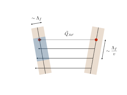
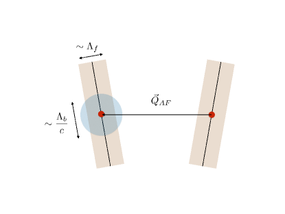
Figure 7: The tilted lines represent patches of Fermi surface connected by the AF ordering vector, where the red dots denote hot spots. The Fermi surfaces are not parallel because of non-zero $v$. (a) Particle-hole excitations of momentum $\vec{Q}_{AF}$ can stay within the low-energy states of energy $E<\Lambda_{f}$ as far as their momenta are within the range of $\Lambda_{f}/v$ from the hot spots. Therefore the phase space available for Landau damping of the collective mode scales as $1/v$ in the small $v$ limit. (b) The shaded region denotes the phase space available for a fermion when scattered by a collective mode of energy less than $\Lambda_{b}$. Since the energy of the boson with momentum $\vec{q}$ scales as $c|\vec{q}|$, a boson with energy less than $\Lambda_{b}$ can transfer momentum up to $\Lambda_{b}/c$ to a fermion. Therefore, the phase space grows as $1/c$ in the small $c$ limit.

Finally, we provide a simple physical picture for why $w=v/c$ emerges as a control parameter. The most important factor is the Landau damping which describes the decay of the collective mode into the particle-hole continuum. As the Fermi surface becomes locally nested near the hot spots in the small $v$ limit, the phase space for the particle-hole excitations that a collective mode can decay into increases as $1/v$. A single boson with a fixed momentum can decay into low-energy particle-hole pairs that lie anywhere along the nested Fermi surface of length $\Lambda_{f}/v$, where $\Lambda_{f}$ is an energy cut-off for the fermionic excitations. This is illustrated in Fig. 7(a). This results in a large screening, which renormalizes the Yukawa vertex to $g^{2}\sim\epsilon v$. As the Fermi surface gets nested, $g$ flows to zero.

The dispersionless particle-hole excitations near the hot spots renormalize the velocity of the collective mode to zero as well, through the mixing between the collective mode and the particle-hole excitations. As the fluctuations of the collective mode become soft, quantum fluctuations are enhanced at low energies. On the other hand, the enhanced quantum fluctuations speeds up the velocity of the collective mode through Fig. 3, and a balance is formed such that $c^{3}\sim g^{2}\sim\epsilon v$ to the leading order in $\epsilon$. As a result, the boson velocity $c$ flows to zero at a much slower rate than $v$.

Now let us consider the feedback of the collective mode on the propagation of fermions, by examining the process where a fermion is scattered by a collecitve mode. With the initial momentum fixed, the fermion does not have access to the entire Fermi surface. Instead it can only scatter into a region allowed by the maximum momentum carried by a collective mode. The available phase space for the scattering scales as $\Lambda_{b}/c$, where $\Lambda_{b}$ is the energy cut-off of the collective mode. This is illustrated in Fig. 7(b). Therefore, the scattering of fermions is controlled by $g^{2}/c\sim\epsilon\,v/c$, where $g^{2}\sim\epsilon v$ is used. As $v/c$ flows to zero in the low energy limit, the scattering of fermions by collective modes becomes negligible. This explains why fermions are largely intact in the small $w$ limit, and $w$ emerges as a control parameter.

VII Conclusion

We extended the earlier one-loop analysis of the antiferromagnetic quantum critical metal based on the dimensional regularization scheme which tunes the number of co-dimensions of the one-dimensional Fermi surface. We show that the IR singularities caused by the emergent quasi-locality rearrange the perturbative series such that a two-loop graph becomes as important as the one-loop graphs in the small $\epsilon$ limit. With the inclusion of this two-loop effect, higher-loop diagrams are systematically suppressed, and the $\epsilon$-expansion is controlled. Furthermore, a ratio between velocities dynamically flows to zero, which has been confirmed in the non-perturbative solution in $2\leq d<3$Schlief et al. (2016, ). The $\epsilon$-expansion provides an independent justification for the ansatz used in the non-perturbative solution.

Appendix A The beta functions and the anomalous dimensions

In this section we summarize the expressions for the beta functions and the anomalous dimensions derived from the minimal subtraction scheme. More details can be found in Ref. Sur and Lee (2015). The renormalized action is given by the sum of the classical action and the counter terms which can be expressed in terms of bare fields and bare couplings,

$$\mathcal{S}_{ren} = \sum_{n=1}^{4}\sum_{\sigma=1}^{N_{c}}\sum_{j=1}^{N_{f}}\int dk_{B}\leavevmode\nobreak\ \bar{\Psi}_{B;n,\sigma,j}(k_{B})\Bigl{[}i\mathbf{\Gamma}\cdot\mathbf{K}_{B}+i\gamma_{d-1}\varepsilon_{n}(\vec{k}_{B};v_{B})\Bigr{]}\Psi_{B;n,\sigma,j}(k)$$ (A1)

$$+\frac{1}{4}\int dq_{B}\leavevmode\nobreak\ \Bigl{[}\left|{\mathbf{Q}_{B}}\right|^{2}+\leavevmode\nobreak\ c_{B}^{2}\left|{\vec{q}_{B}}\right|^{2}\Bigr{]}\mbox{Tr}\left[{\Phi_{B}(-q_{B})\leavevmode\nobreak\ \Phi_{B}(q_{B})}\right]$$

$$+i\frac{g_{B}}{\sqrt{N_{f}}}\sum_{n=1}^{4}\sum_{\sigma,\sigma^{\prime}=1}^{N_{c}}\sum_{j=1}^{N_{f}}\int dk_{B}\,dq_{B}\leavevmode\nobreak\ \Bigl{[}\bar{\Psi}_{B;\bar{n},\sigma,j}(k_{B}+q_{B})\Phi_{B;\sigma,\sigma^{\prime}}(q_{B})\gamma_{d-1}\Psi_{B;n,\sigma^{\prime},j}(k_{B})\Bigr{]}$$

$$+\frac{1}{4}\int dk_{1B}\,dk_{2B}\,dq_{B}\leavevmode\nobreak\ \Bigl{[}u_{1B}\mbox{Tr}\left[{\Phi_{B}(k_{1B}+q_{B})\Phi_{B}(k_{2B}-q_{B})}\right]\mbox{Tr}\left[{\Phi_{B}(-k_{1B})\Phi_{B}(-k_{2B})}\right]$$

$$+u_{2B}\mbox{Tr}\left[{\Phi_{B}(k_{1B}+q_{B})\Phi_{B}(k_{2B}-q_{B})\Phi_{B}(-k_{1B})\Phi_{B}(-k_{2B})}\right]\Bigr{]}.$$

The renormalized quantities are related to the bare ones through $\mathbf{K}=\mathcal{Z}_{\tau}^{-1}\leavevmode\nobreak\ \mathbf{K}_{B}$, $\vec{k}=\vec{k}_{B}$, $\Psi_{n,\sigma,j}(k)=\mathcal{Z}^{-\frac{1}{2}}_{\psi}\leavevmode\nobreak\ \Psi_{B;n,\sigma,j}(k_{B})$, $\Phi(q)=\mathcal{Z}^{-\frac{1}{2}}_{\phi}\leavevmode\nobreak\ \Phi_{B}(q_{B})$, $v=\frac{\mathcal{Z}_{3}}{\mathcal{Z}_{2}}\leavevmode\nobreak\ v_{B}$, $c=\left[\frac{\mathcal{Z}_{\phi}\leavevmode\nobreak\ \mathcal{Z}_{\tau}^{d-1}}{\mathcal{Z}_{5}}\right]^{\frac{1}{2}}\leavevmode\nobreak\ c_{B}$, $g=\frac{\mathcal{Z}_{\psi}\leavevmode\nobreak\ \mathcal{Z}_{\phi}^{\frac{1}{2}}\leavevmode\nobreak\ \mathcal{Z}_{\tau}^{2(d-1)}}{\mathcal{Z}_{6}}\leavevmode\nobreak\ \mu^{-\frac{3-d}{2}}\leavevmode\nobreak\ g_{B}$, $u_{1}=\frac{\mathcal{Z}_{\phi}^{2}\mathcal{Z}_{\tau}^{3(d-1)}}{\mathcal{Z}_{7}}\leavevmode\nobreak\ \mu^{-(3-d)}\leavevmode\nobreak\ u_{1B}$, $u_{2}=\frac{\mathcal{Z}_{\phi}^{2}\mathcal{Z}_{\tau}^{3(d-1)}}{\mathcal{Z}_{8}}\leavevmode\nobreak\ \mu^{-(3-d)}\leavevmode\nobreak\ u_{2B}$, where $\mathcal{Z}_{\tau}=\frac{\mathcal{Z}_{1}}{\mathcal{Z}_{3}}$, $\mathcal{Z}_{\psi}=\mathcal{Z}_{1}\leavevmode\nobreak\ \mathcal{Z}_{\tau}^{-d}$, $\mathcal{Z}_{\phi}=\mathcal{Z}_{4}\leavevmode\nobreak\ \mathcal{Z}_{\tau}^{-(d+1)}$ and $\mathcal{Z}_{n}=1+\mathcal{A}_{n}$. The scaling dimension of $\vec{k}$ is fixed to be $1$. By requiring that the bare quantities are independent of the scale $\mu$, we obtain the dynamical critical exponent, the anomalous dimensions and the beta functions as

$$z =\left[1+(Z^{\prime}_{1,1}-Z^{\prime}_{3,1})\right]^{-1},$$ (A2)

$$\eta_{\psi} =-\frac{\epsilon}{2}\leavevmode\nobreak\ z\left(Z^{\prime}_{1,1}-Z^{\prime}_{3,1}\right)+\frac{1}{2}\leavevmode\nobreak\ z\left(2Z^{\prime}_{1,1}-3Z^{\prime}_{3,1}\right),$$ (A3)

$$\eta_{\phi} =-\frac{\epsilon}{2}\leavevmode\nobreak\ z\left(Z^{\prime}_{1,1}-Z^{\prime}_{3,1}\right)+\frac{1}{2}\leavevmode\nobreak\ z\left(4Z^{\prime}_{1,1}-4Z^{\prime}_{3,1}-Z^{\prime}_{4,1}\right),$$ (A4)

$$\frac{dv}{dl} =-z\leavevmode\nobreak\ v\left(Z^{\prime}_{2,1}-Z^{\prime}_{3,1}\right),$$ (A5)

$$\frac{dc}{dl} =-\frac{1}{2}\leavevmode\nobreak\ z\leavevmode\nobreak\ c\left(2Z^{\prime}_{1,1}-2Z^{\prime}_{3,1}-Z^{\prime}_{4,1}+Z^{\prime}_{5,1}\right),$$ (A6)

$$\frac{dg}{dl} =z\leavevmode\nobreak\ g\left[\frac{\epsilon}{2}+\frac{1}{2}\left(2Z^{\prime}_{3,1}+Z^{\prime}_{4,1}-2Z^{\prime}_{6,1}\right)\right],$$ (A7)

$$\frac{du_{1}}{dl} =z\leavevmode\nobreak\ u_{1}\left[\epsilon-\left(2Z^{\prime}_{1,1}-2Z^{\prime}_{3,1}-2Z^{\prime}_{4,1}+Z^{\prime}_{7,1}\right)\right],$$ (A8)

$$\frac{du_{2}}{dl} =z\leavevmode\nobreak\ u_{2}\left[\epsilon-\left(2Z^{\prime}_{1,1}-2Z^{\prime}_{3,1}-2Z^{\prime}_{4,1}+Z^{\prime}_{8,1}\right)\right],$$ (A9)

where $l=-\ln\mu$ is the logarithmic length scale, and $Z^{\prime}_{n,1}\equiv\left(\frac{1}{2}\leavevmode\nobreak\ g\partial_{g}+u_{i}\partial_{u_{i}}\right)Z_{n,1}$.

Appendix B Computation of the boson self energy at two loops

In this section we compute the quantum corrections to the spatial part of the boson self-energy. Among the two-loop diagrams, only Fig. 3 contributes. It is written as

$$\delta\Gamma_{0,2}^{2L}=-\frac{\mu^{2\epsilon}}{4}\frac{4g^{4}}{N_{c}N_{f}}\int dp\leavevmode\nobreak\ \Upsilon_{0,2}^{2L}(p)\text{Tr}[\Phi(-p)\Phi(p)],$$ (B10)

where

$$\Upsilon_{0,2}^{2L}(p) = \sum_{n}\int dk\,dq\leavevmode\nobreak\ \text{Tr}\left[\gamma_{d-1}G_{n}(q+k)\gamma_{d-1}G_{\bar{n}}(p+q+k)\gamma_{d-1}G_{n}(p+k)\gamma_{d-1}G_{\bar{n}}(k)\right]D(q).$$ (B11)

Since we are interested in the momentum-dependent part, we set $\textbf{P}=0$. We first perform the frequency integrations, which introduces four Feynman parameters $x_{1},x_{2},y_{1},y_{2}$, followed by the spatial integrations. The final expression is given by

$$\Upsilon_{0,2}^{2L;a}(\vec{p})=-\frac{1}{\epsilon}\frac{h_{5}(v,c)}{v^{2}}(p_{x}^{2}+p_{y}^{2})+\mathcal{O}(\epsilon^{0}),$$ (B12)

where $h_{5}(v,c)$ is defined as

$$h_{5}(v,c)=-\frac{2}{(4\pi)^{2}}\int_{0}^{1}dx_{1}\int_{0}^{1-x_{1}}dx_{2}\int_{0}^{1}dy_{1}\int_{0}^{1-y_{1}}dy_{2}\;\left(Av^{2}+B\right),$$ (B13)

with

$$A = -\frac{1}{128\pi^{2}}\Bigg{(}\frac{4\left(b_{1}+b_{2}+b_{3}\right)\left(2\left(1-y_{1}-y_{2}\right)-\left(x_{1}+x_{2}\right)\left(1-2y_{1}-2y_{2}\right)\right)}{\sqrt{a_{1}\,a_{2}\,a_{3}\,a_{4}}\left(1-x_{1}-x_{2}\right)\left(x_{1}+x_{2}\right){}^{2}}$$

$$-\frac{2a_{1}\left(b_{1}+b_{2}+b_{3}\right)\left(a_{2}\,a_{4}\,d_{2,3}+a_{3}\,\left(a_{4}\,d_{2,2}+a_{2}\,d_{2,4}\right)\right)}{\left(a_{1}\,a_{2}\,a_{3}\,a_{4}\right){}^{3/2}}+\frac{4\left(d_{2,5}+d_{2,6}+d_{2,7}\right)}{\sqrt{a_{1}\,a_{2}\,a_{3}\,a_{4}}}$$

$$+\frac{3\left(b_{1}+b_{2}+b_{3}\right)\left(1-y_{1}-y_{2}\right)d_{3,1}}{\sqrt{a_{1}\,a_{2}\,a_{3}}\,a_{4}^{5/2}\left(1-x_{1}-x_{2}\right){}^{2}\left(x_{1}+x_{2}\right){}^{2}}+\frac{a_{1}\left(b_{1}+b_{2}+b_{3}\right)\left(1-y_{1}-y_{2}\right)\left(a_{3}\,d_{3,2}+a_{2}\,d_{3,3}\right)}{\left(a_{1}\,a_{2}\,a_{3}\,a_{4}\right){}^{3/2}\left(1-x_{1}-x_{2}\right){}^{2}\left(x_{1}+x_{2}\right){}^{2}}$$

$$-\frac{2a_{1}\left(1-y_{1}-y_{2}\right)\left(a_{2}\,a_{4}\,\left(d_{3,7}+d_{3,8}+d_{3,9}\right)+a_{3}\,\left(a_{4}\,\left(d_{3,4}+d_{3,5}+d_{3,6}\right)+a_{2}\,\left(d_{3,10}+d_{3,11}+d_{3,12}\right)\right)\right)}{\left(a_{1}\,a_{2}\,a_{3}\,a_{4}\right){}^{3/2}\left(1-x_{1}-x_{2}\right){}^{2}\left(x_{1}+x_{2}\right){}^{2}}\Bigg{)},$$

$$B = A\text{ with }(b_{2}\rightarrow-b_{2},d_{2,6}\rightarrow-d_{2,6},d_{3,5}\rightarrow-d_{3,5},d_{3,8}\rightarrow-d_{3,8},d_{3,11}\rightarrow-d_{3,11}).$$

Here $d_{n,m}$ are defined as

$$d_{2,2} = -c_{1}\left(\left(1-x_{1}-x_{2}\right)\left(x_{1}+x_{2}\right)\right){}^{-2}\left(1-y_{1}-y_{2}\right),$$

$$d_{2,3} = \left(-1+x_{1}+x_{2}-c_{2}\left(-1+c_{4}+x_{1}+x_{2}\right)+c_{4}\left(2-x_{1}-x_{2}+c_{1}\left(-1+c_{4}+x_{1}+x_{2}\right)\right)\right)$$

$$\times\left(-1+y_{1}+y_{2}\right)\left(\left(1-x_{1}-x_{2}\right)\left(x_{1}+x_{2}\right)\right){}^{-2},$$

$$d_{2,4} = \Big{(}c_{1}c_{5}^{2}\left(-1+y_{1}+y_{2}\right)+\left(-1+x_{1}+x_{2}\right)\left(-1+y_{1}+y_{2}\right)-c_{8}^{2}\left(1-c_{1}c_{4}^{2}-x_{1}-x_{2}+c_{2}\left(-1+c_{4}+x_{1}+x_{2}\right)\right.$$

$$+\left.c_{4}\left(-2+x_{1}+x_{2}-c_{1}\left(-1+x_{1}+x_{2}\right)\right)\right)\left(-1+y_{1}+y_{2}\right)-c_{5}\left(-1+x_{1}+x_{2}-c_{8}\left(-2+c_{2}+x_{1}+x_{2}\right)\right.$$

$$+\left.c_{1}\left(2-x_{1}-x_{2}+c_{8}\left(-1+2c_{4}+x_{1}+x_{2}\right)\right)\right)\left(-1+y_{1}+y_{2}\right)+c_{8}\left(-4+3x_{1}+3x_{2}+4y_{1}-4x_{1}y_{1}+x_{1}^{2}y_{1}\right.$$

$$-\left.4x_{2}y_{1}+2x_{1}x_{2}y_{1}+x_{2}^{2}y_{1}+4y_{2}-4x_{1}y_{2}+x_{1}^{2}y_{2}-4x_{2}y_{2}+2x_{1}x_{2}y_{2}+x_{2}^{2}y_{2}+c_{2}\left(-2+x_{1}+x_{2}\right)\left(-1+y_{1}+y_{2}\right)\right.$$

$$-\left.c_{4}\left(1-x_{1}-x_{2}+c_{1}\left(-2+x_{1}+x_{2}\right)\right)\left(-1+y_{1}+y_{2}\right)\right)\Big{)}\left(\left(1-x_{1}-x_{2}\right)\left(x_{1}+x_{2}\right)\right){}^{-2},$$

$$d_{2,5} = \Big{(}c_{11}\left(-c_{9}+c_{8}c_{11}\right)\left(-1+x_{1}+x_{2}\right)\left(x_{1}+x_{2}\right)+\left(c_{1}c_{5}^{2}c_{11}^{2}+c_{1}c_{4}^{2}\left(1+c_{9}-c_{8}c_{11}\right){}^{2}+c_{9}\left(-1+x_{1}+x_{2}\right)\right.$$

$$-\left.\left(-1+c_{2}\right)c_{9}^{2}\left(-1+x_{1}+x_{2}\right)-2c_{8}c_{9}c_{11}\left(-1+x_{1}+x_{2}\right)+c_{5}c_{9}c_{11}\left(2-x_{1}-x_{2}+c_{1}\left(-1+x_{1}+x_{2}\right)\right)\right.$$

$$+\left.c_{2}c_{11}\left(-1+c_{8}c_{11}\right)\left(-2+c_{5}+x_{1}+x_{2}-c_{8}\left(-1+x_{1}+x_{2}\right)\right)+c_{11}\left(-2-c_{11}+x_{1}+c_{11}x_{1}+x_{2}+c_{11}x_{2}\right.\right.$$

$$-\left.\left.c_{9}\left(-2+x_{1}+x_{2}\right){}^{2}+c_{8}^{2}c_{11}\left(-1+x_{1}+x_{2}\right)+c_{8}\left(1-x_{1}-x_{2}+c_{11}\left(-2+x_{1}+x_{2}\right){}^{2}\right)\right)\right.$$

$$-\left.c_{4}\left(1+c_{9}-c_{8}c_{11}\right)\left(-1-c_{11}+2c_{1}c_{11}-2c_{1}c_{5}c_{11}+2c_{8}c_{11}-c_{1}c_{8}c_{11}+c_{2}\left(1+c_{9}-c_{8}c_{11}\right)+c_{11}x_{1}-c_{1}c_{11}x_{1}\right.\right.$$

$$-\left.\left.c_{8}c_{11}x_{1}+c_{1}c_{8}c_{11}x_{1}+c_{11}x_{2}-c_{1}c_{11}x_{2}-c_{8}c_{11}x_{2}+c_{1}c_{8}c_{11}x_{2}+c_{9}\left(-2+x_{1}+x_{2}-c_{1}\left(-1+x_{1}+x_{2}\right)\right)\right)\right.$$

$$-\left.c_{2}c_{9}\left(-1+x_{1}+x_{2}+c_{11}\left(-2+c_{5}+x_{1}+x_{2}-2c_{8}\left(-1+x_{1}+x_{2}\right)\right)\right)-c_{5}c_{11}\left(-1+c_{11}\left(-1+x_{1}+x_{2}\right.\right.\right.$$

$$-\left.\left.\left.c_{8}\left(-2+x_{1}+x_{2}\right)+c_{1}\left(2-x_{1}-x_{2}+c_{8}\left(-1+x_{1}+x_{2}\right)\right)\right)\right)\right)\left(-1+y_{1}+y_{2}\right)\Big{)}\left(\left(1-x_{1}-x_{2}\right)\left(x_{1}+x_{2}\right)\right){}^{-2},$$

$$d_{2,6} = \left(\left(1-x_{1}-x_{2}\right)\left(x_{1}+x_{2}\right)\right){}^{-2}\Big{(}\left(-c_{9}c_{12}+c_{8}c_{11}\left(-1+2c_{12}\right)\right)\left(-1+x_{1}+x_{2}\right)\left(x_{1}+x_{2}\right)+\left(\left(\left(-1+c_{2}\right)c_{8}\right.\right.$$

$$+\left.\left.c_{1}\left(c_{5}-c_{4}c_{8}\right)\right)\left(-\left(-1+c_{5}\right)c_{11}-c_{4}\left(1+c_{9}-c_{8}c_{11}\right)\right)\left(-1+c_{12}\right)-\left(-1+c_{5}-c_{4}c_{8}\right)\left(1+c_{9}-c_{8}c_{11}\right.\right.$$

$$-\left.\left.c_{2}\left(1+c_{9}-c_{8}c_{11}\right)+c_{1}\left(c_{5}c_{11}+c_{4}\left(1+c_{9}-c_{8}c_{11}\right)\right)\right)\left(-1+c_{12}\right)+\left(c_{8}\left(1+2c_{11}-c_{5}c_{11}+c_{1}c_{5}c_{11}\right.\right.\right.$$

$$-\left.\left.\left.2c_{8}c_{11}+c_{2}\left(-1+\left(-1+2c_{8}\right)c_{11}\right)-\left(-1+c_{1}\right)c_{4}\left(-1+\left(-1+2c_{8}\right)c_{11}\right)\right)+c_{9}\left(-1+\left(-1+c_{1}\right)c_{5}\left(-1+c_{12}\right)\right.\right.\right.$$

$$+\left.\left.\left.2\left(-1+c_{2}+c_{4}-c_{1}c_{4}\right)c_{8}\left(-1+c_{12}\right)+2c_{12}-c_{2}c_{12}-c_{4}c_{12}+c_{1}c_{4}c_{12}\right)+\left(-1+c_{8}\right)\left(\left(-1+c_{2}-\left(-1+c_{1}\right)c_{4}\right)c_{12}\right.\right.\right.$$

$$+\left.\left.\left.c_{11}\left(1+\left(-1+c_{1}\right)c_{5}-2\left(1+\left(-1+c_{1}\right)c_{5}+\left(-1+c_{2}+c_{4}-c_{1}c_{4}\right)c_{8}\right)c_{12}\right)\right)\right)\left(1-x_{1}-x_{2}\right)\right.$$

$$-\left.c_{8}c_{11}\left(-1+c_{12}\right)\left(-1+x_{1}+x_{2}\right){}^{2}+\left(c_{9}-c_{8}c_{11}\right)c_{12}\left(-1+x_{1}+x_{2}\right){}^{2}\right)\left(1-y_{1}-y_{2}\right)\Big{)},$$

$$d_{2,7} = \left(\left(1-x_{1}-x_{2}\right)\left(x_{1}+x_{2}\right)\right){}^{-2}\Big{(}\left(\left(-1+c_{12}\right)\left(c_{1}\left(c_{5}-c_{4}c_{8}\right)\left(1+c_{5}\left(-1+c_{12}\right)-\left(-1+c_{4}\right)c_{8}\left(-1+c_{12}\right)-2c_{12}\right)\right.\right.$$

$$-\left.\left.\left(1+c_{2}\left(-1+c_{4}\right)-2c_{4}\right)c_{8}^{2}\left(-1+c_{12}\right)+\left(-1+c_{5}\right)c_{12}+c_{8}\left(-2+c_{2}\left(1+c_{5}\left(-1+c_{12}\right)-2c_{12}\right)-2c_{5}\left(-1+c_{12}\right)\right.\right.\right.$$

$$+\left.\left.\left.4c_{12}-c_{4}c_{12}\right)\right)-c_{8}x_{1}+\left(1-c_{2}+\left(-1+c_{1}\right)c_{4}\right)c_{8}^{2}x_{1}+\left(-1+c_{1}\right)c_{5}\left(-1+c_{8}\right)c_{12}x_{1}+c_{8}c_{12}x_{1}-2c_{8}^{2}c_{12}x_{1}\right.$$

$$-\left.\left(-1+c_{1}\right)c_{5}c_{8}\left(-1+c_{12}\right)c_{12}x_{1}+\left(1-c_{2}+\left(-1+c_{1}\right)c_{4}\right)c_{8}^{2}c_{12}^{2}x_{1}+c_{12}\left(-1+\left(1+\left(-1+c_{1}\right)c_{5}\right)c_{12}\right)x_{1}\right.$$

$$+\left.c_{8}\left(-1+c_{12}\right)x_{2}+\left(1-c_{2}+\left(-1+c_{1}\right)c_{4}\right)c_{8}^{2}\left(-1+c_{12}\right){}^{2}x_{2}+\left(1+\left(-1+c_{1}\right)c_{5}\right)\left(-1+c_{12}\right)c_{12}x_{2}\right.$$

$$+\left.c_{8}\left(\left(c_{2}-\left(-1+c_{1}\right)c_{4}\right)c_{12}\left(\left(-1+2c_{8}+c_{12}\right)x_{1}+\left(-1+c_{12}\right)x_{2}\right)-\left(-1+c_{1}\right)c_{5}\left(x_{1}+\left(-1+c_{12}\right){}^{2}x_{2}\right)\right)\right)\left(-1+y_{1}+y_{2}\right)$$

$$+c_{8}\left(-1+c_{12}\right)c_{12}\left(x_{1}+x_{2}\right)\left(3+\left(-4+x_{1}+x_{2}\right)y_{1}+\left(-4+x_{1}+x_{2}\right)y_{2}\right)\Big{)},$$

$$d_{3,1} = c_{8}\left(1-c_{5}+c_{4}c_{8}\right)\left(-\left(-1+c_{2}\right)c_{8}+c_{1}\left(-c_{5}+c_{4}c_{8}\right)\right),$$

$$d_{3,2} = c_{1}c_{8},$$

$$d_{3,3} = 1-c_{5}+c_{2}\left(-1+c_{5}-3c_{4}c_{8}\right)+c_{4}\left(3c_{8}+c_{1}\left(1-2c_{5}+3c_{4}c_{8}\right)\right),$$

$$d_{3,4} = c_{1}c_{11}\left(-c_{9}+c_{8}c_{11}\right),$$

$$d_{3,5} = -c_{1}\left(c_{8}c_{11}\left(1-2c_{12}\right)+c_{9}c_{12}\right),$$

$$d_{3,6} = c_{1}c_{8}\left(-1+c_{12}\right)c_{12},$$

$$d_{3,7} = c_{11}\left(\left(-1+c_{2}\right)\left(-1+c_{5}\right)c_{11}+c_{1}c_{4}^{2}\left(-2-3c_{9}+3c_{8}c_{11}\right)\right.$$

$$+\left.c_{4}\left(-2-3c_{9}+c_{1}c_{11}-2c_{1}c_{5}c_{11}+3c_{8}c_{11}+c_{2}\left(2+3c_{9}-3c_{8}c_{11}\right)\right)\right),$$

$$d_{3,8} = c_{4}\left(-1+c_{2}-c_{1}c_{4}\right)\left(2+3c_{9}\right)c_{12}-\left(-1+c_{5}-3c_{4}c_{8}-c_{1}c_{4}\left(1-2c_{5}+3c_{4}c_{8}\right)+c_{2}\left(1-c_{5}+3c_{4}c_{8}\right)\right)c_{11}\left(-1+2c_{12}\right),$$

$$d_{3,9} = -\left(-1+c_{5}-3c_{4}c_{8}-c_{1}c_{4}\left(1-2c_{5}+3c_{4}c_{8}\right)+c_{2}\left(1-c_{5}+3c_{4}c_{8}\right)\right)\left(-1+c_{12}\right)c_{12},$$

$$d_{3,10} = c_{1}c_{4}^{2}c_{8}+\left(1-c_{5}+c_{2}\left(-1+c_{5}-3c_{4}c_{8}\right)+c_{4}\left(3c_{8}+c_{1}\left(1-2c_{5}+3c_{4}c_{8}\right)\right)\right)c_{9}^{2}+3c_{8}\left(-1+c_{5}-c_{4}c_{8}\right)c_{11}\left(1-c_{2}\right.$$

$$+\left.2\left(c_{1}c_{5}+\left(-1+c_{2}-c_{1}c_{4}\right)c_{8}\right)c_{11}\right)+c_{9}\left(\left(-1+c_{2}\right)\left(-1+c_{5}-2c_{4}c_{8}\right)-3\left(\left(-1+c_{2}\right)c_{8}\left(-2+2c_{5}-3c_{4}c_{8}\right)\right.\right.$$

$$+\left.\left.c_{1}\left(c_{5}^{2}+c_{4}c_{8}\left(2+3c_{4}c_{8}\right)-c_{5}\left(1+4c_{4}c_{8}\right)\right)\right)c_{11}\right)-c_{4}\left(c_{1}\left(-1+2c_{5}\right)c_{9}+c_{8}\left(-1+c_{2}+2\left(-1+c_{2}-2c_{1}c_{4}\right)c_{9}\right.\right.$$

$$+\left.\left.3\left(-\left(-1+c_{2}\right)c_{8}+c_{1}\left(1-2c_{5}+2c_{4}c_{8}\right)\right)c_{11}\right)\right),$$

$$d_{3,11} = -c_{1}\left(-1+c_{5}\right)c_{5}c_{9}\left(-2+3c_{12}\right)+3c_{4}\left(1-c_{2}+c_{1}c_{4}\right)c_{8}^{3}c_{11}\left(-3+4c_{12}\right)+c_{8}^{2}\left(-c_{1}c_{4}^{2}\left(2+3c_{9}\right)\left(-2+3c_{12}\right)\right.$$

$$+\left.3\left(-1+c_{2}\right)\left(-1+c_{5}\right)c_{11}\left(-3+4c_{12}\right)+c_{4}\left(4-9c_{1}c_{11}+18c_{1}c_{5}c_{11}+c_{9}\left(6-9c_{12}\right)-6c_{12}+12c_{1}c_{11}c_{12}\right.\right.$$

$$-\left.\left.24c_{1}c_{5}c_{11}c_{12}+c_{2}\left(2+3c_{9}\right)\left(-2+3c_{12}\right)\right)\right)+c_{8}\left(\left(-1+c_{5}\right)\left(1+2c_{9}\right)\left(-2+3c_{12}\right)-c_{2}\left(-1+c_{5}\right)\left(1+2c_{9}\right)\left(-2+3c_{12}\right)\right.$$

$$+\left.c_{1}\left(c_{4}\left(-1+2c_{5}\right)\left(1+2c_{9}\right)\left(-2+3c_{12}\right)+3\left(-1+c_{5}\right)c_{5}c_{11}\left(-3+4c_{12}\right)\right)\right),$$

$$d_{3,12} = 3c_{8}\left(1-c_{5}+c_{4}c_{8}\right)\left(-\left(-1+c_{2}\right)c_{8}+c_{1}\left(-c_{5}+c_{4}c_{8}\right)\right)\left(1-3c_{12}+2c_{12}^{2}\right),$$

where $a_{n}$, $b_{n}$ and $c_{n}$ are given by

$$a_{1} = -\mathcal{X}_{1}\left(-1+y_{1}+y_{2}\right)\left(4v^{2}\left(-1+x_{1}+x_{2}\right)\left(x_{1}+x_{2}\right)\right)^{-1},$$

$$a_{2} = -\mathcal{X}_{2}\left(-1+y_{1}+y_{2}\right)\left(\mathcal{X}_{1}\left(-1+x_{1}+x_{2}\right)\left(x_{1}+x_{2}\right)\right)^{-1},$$

$$a_{3} = \mathcal{X}_{3}\left(\left(x_{1}+x_{2}\right)\mathcal{X}_{2}\right)^{-1},$$

$$a_{4} = \mathcal{X}_{4}\left(\left(x_{1}+x_{2}\right)\mathcal{X}_{3}\right)^{-1},$$

$$b_{1} = \mathcal{X}_{4}^{-1}\,c^{2}x_{1}y_{1}\left(-1+y_{1}+y_{2}\right)\left(c^{2}\left(-1+x_{1}\right)x_{1}y_{2}+\left(-1+c^{2}-v^{2}\right)x_{2}^{2}y_{2}+x_{2}\left(-c^{2}+c^{2}y_{1}+\left(-1+2c^{2}-v^{2}\right)x_{1}y_{2}\right)\right),$$

$$b_{2} = -\mathcal{X}_{4}^{-1}\,2c^{2}\left(-1+v^{2}\right)x_{1}x_{2}\left(x_{1}+x_{2}\right)y_{1}y_{2}\left(-1+y_{1}+y_{2}\right),$$

$$b_{3} = \mathcal{X}_{4}^{-1}\,c^{2}x_{2}\left(\left(-1+c^{2}-v^{2}\right)x_{1}^{2}y_{1}+c^{2}\left(-1+x_{2}\right)x_{2}y_{1}+x_{1}\left(\left(-1+2c^{2}-v^{2}\right)x_{2}y_{1}+c^{2}\left(-1+y_{2}\right)\right)\right)y_{2}\left(-1+y_{1}+y_{2}\right),$$

$$c_{1} = -\mathcal{X}_{1}^{-1}\,c^{2}\left(-1+v^{2}\right)\left(-1+x_{1}+x_{2}\right),$$

$$c_{2} = -\mathcal{X}_{1}^{-1}\,4v^{2}x_{1},$$

$$c_{4} = c_{1}\,\mathcal{X}_{1}\,\mathcal{X}_{2}^{-1}\,x_{1},$$

$$c_{5} = -\mathcal{X}_{1}\,\mathcal{X}_{2}^{-1}\,x_{2},$$

$$c_{8} = \mathcal{X}_{3}^{-1}\,c^{2}\left(-1+v^{2}\right)x_{1}x_{2}\left(-1+y_{1}+y_{2}\right),$$

$$c_{9} = \mathcal{X}_{3}^{-1}\,c^{2}x_{1}\left(c^{2}-c^{2}x_{1}+\left(1-c^{2}+v^{2}\right)x_{2}\right)\left(-1+y_{1}+y_{2}\right),$$

$$c_{11} = -\mathcal{X}_{4}^{-1}\,\left(c^{2}\left(-1+v^{2}\right)x_{1}x_{2}\left(x_{1}+x_{2}\right)y_{1}\left(-1+y_{1}+y_{2}\right)\right),$$

$$c_{12} = -\mathcal{X}_{4}^{-1}\,\left(c^{2}x_{2}\left(\left(1-c^{2}+v^{2}\right)x_{1}^{2}y_{1}-c^{2}\left(-1+x_{2}\right)x_{2}y_{1}+x_{1}\left(\left(1-2c^{2}+v^{2}\right)x_{2}y_{1}-c^{2}\left(-1+y_{2}\right)\right)\right)\left(-1+y_{1}+y_{2}\right)\right)$$

with

$$\mathcal{X}_{1} = \left(c^{2}+\left(-4+c^{2}\right)v^{2}\right)x_{1}+c^{2}\left(1+v^{2}\right)\left(-1+x_{2}\right),$$

$$\mathcal{X}_{2} = c^{2}\left(-1+c^{2}-v^{2}\right)x_{1}^{2}+c^{2}\left(-1+x_{2}\right)\left(-c^{2}+\left(-1+c^{2}-v^{2}\right)x_{2}\right)+x_{1}\left(c^{2}\left(1-2c^{2}+v^{2}\right)+2\left(c^{4}+2v^{2}-c^{2}\left(1+v^{2}\right)\right)x_{2}\right),$$

$$\mathcal{X}_{3} = c^{2}\left(-1+c^{2}-v^{2}\right)x_{1}^{3}y_{1}+c^{2}\left(-1+x_{2}\right)x_{2}\left(-c^{2}+\left(-1+c^{2}-v^{2}\right)x_{2}\right)y_{1}+x_{1}\left(\left(3c^{4}+4v^{2}-3c^{2}\left(1+v^{2}\right)\right)x_{2}^{2}y_{1}\right.$$

$$\left.+c^{2}x_{2}\left(\left(1-3c^{2}+v^{2}\right)y_{1}+\left(-1+c^{2}-v^{2}\right)\left(-1+y_{2}\right)\right)-c^{4}\left(-1+y_{2}\right)\right)+x_{1}^{2}\left(\left(c^{2}\left(1-c^{2}+v^{2}\right)\right.\right.$$

$$\left.\left.+\left(3c^{4}+4v^{2}-3c^{2}\left(1+v^{2}\right)\right)x_{2}\right)y_{1}+c^{4}\left(-1+y_{2}\right)\right),$$

$$\mathcal{X}_{4} = c^{2}\left(-1+c^{2}-v^{2}\right)x_{1}^{4}y_{1}y_{2}+x_{1}^{3}\left(\left(c^{2}\left(1-c^{2}+v^{2}\right)+4\left(-1+c^{2}\right)\left(c^{2}-v^{2}\right)x_{2}\right)y_{1}+c^{4}\left(-1+y_{2}\right)\right)y_{2}$$

$$+c^{2}\left(-1+x_{2}\right)x_{2}^{2}y_{1}\left(-c^{2}+c^{2}y_{1}+\left(-1+c^{2}-v^{2}\right)x_{2}y_{2}\right)+x_{1}x_{2}\left(c^{2}\left(-1+2c^{2}-v^{2}\right)x_{2}y_{1}^{2}\right.$$

$$\left.+c^{2}\left(-1+y_{2}\right)\left(-c^{2}+\left(-1+c^{2}-v^{2}\right)x_{2}y_{2}\right)+y_{1}\left(4\left(-1+c^{2}\right)\left(c^{2}-v^{2}\right)x_{2}^{2}y_{2}+c^{4}\left(-1+2y_{2}\right)\right.\right.$$

$$\left.\left.+c^{2}x_{2}\left(1-2c^{2}+v^{2}+\left(1-3c^{2}+v^{2}\right)y_{2}\right)\right)\right)+x_{1}^{2}\left(2\left(3c^{4}+4v^{2}-3c^{2}\left(1+v^{2}\right)\right)x_{2}^{2}y_{1}y_{2}-c^{4}\left(-1+y_{2}\right)y_{2}\right.$$

$$\left.+c^{2}x_{2}\left(\left(-1+c^{2}-v^{2}\right)y_{1}^{2}+\left(-1+2c^{2}-v^{2}\right)\left(-1+y_{2}\right)y_{2}+y_{1}\left(1-c^{2}+v^{2}+\left(1-3c^{2}+v^{2}\right)y_{2}\right)\right)\right).$$

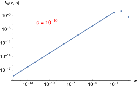
Figure B1: The dots represent $h_{5}(v,c)$ evaluated as a function of $w=v/c$ at fixed $c=10^{-10}$. The line represents $L(w)=5.7\times 10^{-4}\,w$. It is noted that $h_{5}(v,c)$ deviates from the line beyond $w\sim 0.1$.

To extract the leading behavior of $h_{5}(v,c)$ in the limit $v,c,w\equiv v/c$ are small, we approximate the integrand in $h_{5}(v,c)$ by its leading order term in this limit. This gives $h_{5}(v,c)=h_{5}^{*}\,w$ with $h_{5}^{*}\approx 5.7\times 10^{-4}$ to the leading order in $v,c,w$. In Fig. (B1), we show the full $h_{5}(v,c)$ as a function of $w=\frac{v}{c}$ for a small value of $c$, which confirms the linear behavior in the small $w$ limit. The two-loop contribution to the quantum effective action is

$$\delta\Gamma_{0,2}^{2L}=\frac{1}{\epsilon}\frac{4}{N_{c}N_{f}}\frac{g^{4}}{v^{2}c^{2}}h_{5}(v,c)\int dp\leavevmode\nobreak\ \frac{1}{4}c^{2}|\vec{p}|^{2}\text{Tr}[\Phi(-p)\Phi(p)]\leavevmode\nobreak\ +\leavevmode\nobreak\ \mathcal{O}(\epsilon^{0}).$$ (B14)

Combining Eq.(B14) with the one-loop quantum effective action obtained in Ref. Sur and Lee (2015), we obtain the counter terms as

$$Z_{1,1} = -\frac{(N_{c}^{2}-1)}{4\pi^{2}N_{c}N_{f}}\leavevmode\nobreak\ \frac{g^{2}}{c}\leavevmode\nobreak\ h_{1}(v,c),$$ (B15)

$$Z_{2,1} = \frac{(N_{c}^{2}-1)}{4\pi^{2}N_{c}N_{f}}\leavevmode\nobreak\ \frac{g^{2}}{c}\leavevmode\nobreak\ h_{2}(v,c),$$ (B16)

$$Z_{3,1} = -Z_{2,1},$$ (B17)

$$Z_{4,1} = -\frac{1}{4\pi}\leavevmode\nobreak\ \frac{g^{2}}{v},$$ (B18)

$$Z_{5,1} = -\frac{4}{N_{c}N_{f}}\frac{g^{4}}{v^{2}c^{2}}h_{5}(v,c),$$ (B19)

$$Z_{6,1} = -\frac{1}{8\pi^{3}N_{c}N_{f}}\leavevmode\nobreak\ \frac{g^{2}}{c}\leavevmode\nobreak\ h_{3}(v,c),$$ (B20)

$$Z_{7,1} = \frac{1}{2\pi^{2}c^{2}}\left[(N_{c}^{2}+7)u_{1}+2\left(2N_{c}-\frac{3}{N_{c}}\right)u_{2}+3\left(1+\frac{3}{N_{c}^{2}}\right)\frac{u_{2}^{2}}{u_{1}}\right],$$ (B21)

$$Z_{8,1} = \frac{1}{2\pi^{2}c^{2}}\left[12u_{1}+2\left(N_{c}-\frac{9}{N_{c}}\right)u_{2}\right].$$ (B22)

Here $h_{1}(v,c)$, $h_{2}(v,c)$, and $h_{3}(v,c)$ are given bySur and Lee (2015)

$$h_{1}(v,c) = \int_{0}^{1}dx\,\sqrt{\frac{1-x}{c^{2}+(1+v^{2}-c^{2})x}}=\frac{\pi\left(1+v^{2}\right)-2c\sqrt{1-c^{2}+v^{2}}-i\left(1+v^{2}\right)\left(\log\left(1+v^{2}\right)-2\log\left(ic+\sqrt{1-c^{2}+v^{2}}\right)\right)}{2\left(1-c^{2}+v^{2}\right)^{3/2}},$$

$$h_{2}(v,c) = c^{2}\int_{0}^{1}dx\,\sqrt{\frac{1-x}{(c^{2}+(1+v^{2}-c^{2})x)^{3}}}=-\frac{c\left(-2\sqrt{1-c^{2}+v^{2}}-ic\left(\log\left(-1-v^{2}\right)-2\log\left(ic+\sqrt{1-c^{2}+v^{2}}\right)\right)\right)}{\left(1-c^{2}+v^{2}\right)^{3/2}},$$

$$h_{3}(v,c) = \int_{0}^{1}dx_{1}\int_{0}^{1-x_{1}}dx_{2}\frac{\pi c\left(8v^{2}x_{1}x_{2}+2c^{4}\left(-1+x_{1}+x_{2}\right){}^{2}-c^{2}\left(-1+x_{1}+x_{2}\right)\left(1+2x_{1}+2x_{2}+v^{2}\left(-1+2x_{1}+2x_{2}\right)\right)\right)}{\left(4v^{2}x_{1}x_{2}+c^{4}\left(-1+x_{1}+x_{2}\right){}^{2}-c^{2}\left(1+v^{2}\right)\left(-1+x_{1}+x_{2}\right)\left(x_{1}+x_{2}\right)\right){}^{3/2}}.$$

From the expressions for $Z_{n,1}$, we obtain the beta functions for $\lambda\equiv\frac{g^{2}}{v},x\equiv\frac{g^{2}}{c^{3}},w\equiv\frac{v}{c},\kappa_{i}\equiv\frac{u_{i}}{c^{2}}$,

$$\frac{d\lambda}{dl} = z\leavevmode\nobreak\ \lambda\left(\epsilon-\frac{\lambda}{4\pi}+\frac{1}{4\pi^{3}N_{c}N_{f}}\leavevmode\nobreak\ \lambda w\leavevmode\nobreak\ h_{3}(v,c)\right),$$ (B23)

$$\frac{dx}{dl} = z\leavevmode\nobreak\ x\left(\epsilon-\frac{3(N_{c}^{2}-1)}{4\pi^{2}N_{c}N_{f}}\leavevmode\nobreak\ \lambda w\leavevmode\nobreak\ h_{1}(v,c)+\frac{(N_{c}^{2}-1)}{4\pi^{2}N_{c}N_{f}}\leavevmode\nobreak\ \lambda w\leavevmode\nobreak\ h_{2}(v,c)+\frac{\lambda}{8\pi}-\frac{12}{N_{c}N_{f}}\frac{\lambda x}{w}h_{5}(v,c)+\frac{\lambda w\leavevmode\nobreak\ h_{3}(v,c)}{4\pi^{3}N_{c}N_{f}}\right),$$ (B24)

$$\frac{dw}{dl} = \frac{1}{2}\leavevmode\nobreak\ z\leavevmode\nobreak\ w\left(-\frac{(N_{c}^{2}-1)}{2\pi^{2}N_{c}N_{f}}\leavevmode\nobreak\ \lambda w\leavevmode\nobreak\ h_{1}(v,c)-\frac{(N_{c}^{2}-1)}{2\pi^{2}N_{c}N_{f}}\leavevmode\nobreak\ \lambda w\leavevmode\nobreak\ h_{2}(v,c)+\frac{\lambda}{4\pi}-\frac{8}{N_{c}N_{f}}\frac{\lambda x}{w}h_{5}(v,c)\right),$$ (B25)

$$\frac{d\kappa_{1}}{dl} = z\leavevmode\nobreak\ \kappa_{1}\left(\epsilon-\frac{\lambda}{4\pi}-\frac{8}{N_{c}N_{f}}\frac{\lambda x}{w}h_{5}(v,c)-\frac{1}{2\pi^{2}}\left((N_{c}^{2}+7)\kappa_{1}+2\left(2N_{c}-\frac{3}{N_{c}}\right)\kappa_{2}+3\left(1+\frac{3}{N_{c}^{2}}\right)\frac{\kappa_{2}^{2}}{\kappa_{1}}\right)\right),$$ (B26)

$$\frac{d\kappa_{2}}{dl} = z\leavevmode\nobreak\ \kappa_{2}\left(\epsilon-\frac{\lambda}{4\pi}-\frac{8}{N_{c}N_{f}}\frac{\lambda x}{w}h_{5}(v,c)-\frac{1}{2\pi^{2}}\left(12\kappa_{1}+2\left(N_{c}-\frac{9}{N_{c}}\right)\kappa_{2}\right)\right).$$ (B27)

The leading order behavior of $h_{i}(v,c)$ in the limit of small $v,c,w$ are $h_{1}(v,c)=\frac{\pi}{2}$, $h_{2}(v,c)=2c$, $h_{3}(v,c)=2\pi^{2}$.

Appendix C Upper bound of higher-loop diagrams

Here we estimate the magnitude of higher-loop diagrams without self-energy insertions at the M1L fixed point. Since $\kappa_{i}=0$ at the fixed point, we consider diagrams made of Yukawa vertices only. The discussion closely follows Appendix A of Ref. Schlief et al. (2016), and we will be brief here. A general $L$-loop diagram can be written as

$$I\sim g^{V}\int\prod_{r=1}^{L}dp_{r}\left(\prod_{l=1}^{I_{f}}\frac{1}{\textbf{K}_{l}\cdot\boldsymbol{\Gamma}+\varepsilon_{n_{l}}(k_{l})\gamma_{d-1}}\right)\left(\prod_{m=1}^{I_{b}}\frac{1}{|\textbf{Q}_{m}|^{2}+c^{2}(q_{m,x}^{2}+q_{m,y}^{2})}\right).$$ (C28)

Here $V$ is the number of Yukawa vertices. $I_{f},I_{b}$ are the number of fermion and boson propagators, respectively. $p_{r}$’s represent the internal momenta. $k_{l}$ ($q_{m}$) is the momentum that flows through the $l$-th fermion ($m$-th boson) propagator, which is given by a linear combination of the internal and external momenta. $n_{l}$ is the patch index of the $l$-th fermion line. Without loss of generality, we can focus on diagrams that involve only patches $1$ and $3$. We are ignoring the $\gamma$ matrices coming from the Yukawa vertices as they play no role in the estimation.

The dependence of $k_{l}$ and $q_{m}$ on the internal momenta is determined by the choice of loops. One can choose the loop momenta such that $L-L_{f}$ boson propagators become exclusive propagators, in the sense that each of them depends exclusively on only one internal momentum, where $L_{f}$ is the number of fermion loops. Since the limit of small $v,c,w$ does not affect the frequency integrations, we focus on the spatial parts of the propagators. The integrations for $p_{r,x},p_{r,y}$ in Eq.(C28) can be written as

$$I\sim g^{V}\int\displaystyle\prod_{r=1}^{L}dp_{r,x}dp_{r,y}\left(\displaystyle\prod_{m=1}^{L-L_{f}}\frac{1}{(cp_{m,x})^{2}+(cp_{m,y})^{2}}\right)\left(\displaystyle\prod_{l=1}^{I_{f}}\frac{1}{E_{l}(p)}\right)R[p].$$

Here we have dropped the frequency variables and all the $\gamma$ matrices. The first group represents the exclusive boson propagators for the $L-L_{f}$ non-fermion loops. The second group represents all fermion propagators, and the energy of the fermion is written $E_{l}(p)\equiv\varepsilon_{l}(k_{l}(p))$, where $k_{l}(p)$ is the momentum that flows through the $l$-th fermion propagator which is a function of internal momenta. $R[p]$ represents the remaining boson propagators in the diagram.

Now we change variables in a way that the divergence in the small $v,c$ limit becomes manifest. The first $L-L_{f}$ variables are chosen to be $p^{{}^{\prime}}_{i}\equiv cp_{i,x}$ with $1<i\leq L-L_{f}$. The remaining $L+L_{f}$ variables are chosen among $\{E_{l}(p)\}$. $\{p^{\prime}_{i},E_{l}(p)\}$ are expressed in terms of $\{vp_{r,x},p_{r,y}\}$ as

$$\left(\begin{array}[]{c}p^{{}^{\prime}}_{1}\\ p^{{}^{\prime}}_{2}\\ \vdots\\ p^{{}^{\prime}}_{L-L_{f}}\\ \\ E_{1}\\ E_{2}\\ \vdots\\ E_{I_{f}}\end{array}\right)=\left(\begin{array}[]{cc}\frac{c}{v}{\mathbb{I}}_{L-L_{f}}&0\\ {\mathbb{A}}&{\mathbb{V}}\end{array}\right)\left(\begin{array}[]{c}vp_{1,x}\\ vp_{2,x}\\ \vdots\\ vp_{L-L_{f},x}\\ \\ vp_{L-L_{f}+1,x}\\ vp_{L-L_{f}+2,x}\\ \vdots\\ vp_{L,x}\\ p_{1,y}\\ p_{2,y}\\ \vdots\\ p_{L,y}\\ \end{array}\right).$$ (C53)

Here, ${\mathbb{I}}_{a}$ is the $a\times a$ identity matrix. $\mathbb{A}$ is an $I_{f}\times(L-L_{f})$ matrix whose matrix elements are given by $\mathbb{A}_{n,i}=\frac{1}{v}\frac{\partial E_{n}}{\partial p_{i,x}}$ with $1\leq n\leq I_{f}$ and $1\leq i\leq L-L_{f}$. $\mathbb{V}$ is an $I_{f}\times(L+L_{f})$ matrix whose first $L_{f}$ columns are given by $\mathbb{V}_{n,a-(L-L_{f})}=\frac{1}{v}\frac{\partial E_{n}}{\partial p_{a,x}}$ for $L-L_{f}+1\leq a\leq L$ while the remaining $L$ columns are given by $\mathbb{V}_{n,b+L_{f}}=\frac{\partial E_{n}}{\partial p_{b,y}}$ for $1\leq b\leq L$. In Ref. Schlief et al. (2016) it is shown that the $L+L_{f}$ column vectors of $\mathbb{V}$ are linearly independent. Therefore, there exist $L+L_{f}$ row vectors of $\mathbb{V}$ that are linearly independent, which we label to be the $l_{k}$-th rows with $k=1,...,(L+L_{f})$. Let $\tilde{\mathbb{V}}$ be the $(L+L_{f})\times(L+L_{f})$ matrix consisting of these rows. Then we define $p^{{}^{\prime}}_{L-L_{f}+k}\equiv E_{l_{k}}$ with $k=1,...,(L+L_{f})$ as the remaining $(L+L_{f})$ integration variables. The new momentum variables are given in terms of the old variables by

$$\left(\begin{array}[]{c}p^{{}^{\prime}}_{1}\\ p^{{}^{\prime}}_{2}\\ \vdots\\ p^{{}^{\prime}}_{2L}\end{array}\right)=\left(\begin{array}[]{cc}\frac{c}{v}{\mathbb{I}}_{L-L_{f}}&0\\ \tilde{{\mathbb{A}}}&\tilde{{\mathbb{V}}}\end{array}\right)\left(\begin{array}[]{c}vp_{1,x}\\ vp_{2,x}\\ \vdots\\ vp_{L-L_{f},x}\\ \\ vp_{L-L_{f}+1,x}\\ vp_{L-L_{f}+2,x}\\ \vdots\\ vp_{L,x}\\ p_{1,y}\\ p_{2,y}\\ \vdots\\ p_{L,y}\\ \end{array}\right),$$ (C73)

where $\tilde{\mathbb{A}}$ is the collection of the $l_{k}$-th rows of $\mathbb{A}$, with $k=1,...,(L+L_{f})$. The Jacobian of this change of variables is given by $Y^{-1}c^{-(L-L_{f})}v^{-L_{f}}$, where $Y=|\det\tilde{\mathbb{V}}|$ is a numerical constant independent of $v,c$. $Y$ is nonzero because $\tilde{\mathbb{V}}$ is invertible. In the new basis, it is manifest that for every integration variable $p_{r}^{{}^{\prime}}$, there is one propagator that guarantees the integrand decays at least as $1/p_{r}^{{}^{\prime}}$, in the limit $c,v\rightarrow 0$. Since there is no sub-diagram with a positive degree of UV divergence, the integrations over $p_{r}^{{}^{\prime}}$ are at most logarithmically divergent in the UV cut-off or $v,c$. Therefore, the diagram is bounded by

$$I\sim\frac{g^{V}}{v^{L_{f}}c^{L-L_{f}}},$$ (C74)

up to potential logarithmic corrections in $v$ and $c$.

Appendix D Beyond the modified one-loop order

In this appendix, we consider the effects of higher-loop diagrams in the small $w$ limit. To the leading order in $w$, the higher-loop diagrams that need to be considered are the M1L diagrams in which the boson propagator is dressed with the self-energy insertions in Figs. 2(a) and 3. An insertion of the self-energy in Fig. 2(a) adds one power of $\lambda$ to $Z_{n,1}$, while an insertion of the self-energy in Fig. 3 adds one power of $\lambda x$, up to logarithmic corrections in $c,v$ for both insertions. We write the general form of the counter terms from the higher-loop diagrams as

$$Z_{1,1} = \lambda w\sum_{n,m=0}^{\infty}\lambda^{n+m}x^{m}a_{n,m}(c,v),$$ (D75)

$$Z_{2,1} = \frac{(\lambda w)^{\frac{3}{2}}}{x^{\frac{1}{2}}}\sum_{n,m=0}^{\infty}\lambda^{n+m}x^{m}b_{n,m}(c,v),$$ (D76)

$$Z_{3,1} = -Z_{2,1},$$ (D77)

$$Z_{4,1} = -\frac{1}{4\pi}\lambda,$$ (D78)

$$Z_{5,1} = \lambda x\sum_{n,m=0}^{\infty}\lambda^{n+m}x^{m}h_{n,m}(c,v),$$ (D79)

$$Z_{6,1} = \lambda w\sum_{n,m=0}^{\infty}\lambda^{n+m}x^{m}r_{n,m}(c,v).$$ (D80)

Here, $a_{n,m}(c,v),b_{n,m}(c,v),h_{n,m}(c,v),r_{n,m}(c,v)$ are functions that grow at most logarithmically in $c,v$. For $n=m=0$, they are independent of $c,v$, and given by $a_{0,0}(c,v)=-\frac{(N_{c}^{2}-1)}{8\pi N_{c}N_{f}}$, $b_{0,0}(c,v)=\frac{(N_{c}^{2}-1)}{2\pi^{2}N_{c}N_{f}}$, $h_{0,0}(c,v)=-\frac{4\,h_{5}^{*}}{N_{c}N_{f}}$, $r_{0,0}(c,v)=-\frac{1}{4\pi N_{c}N_{f}}$. The relation $Z_{2,1}=-Z_{3,1}$ still holds because the external momentum can be passed through a single fermion line with the opposite patch index to the external lines.

We first establish that the fixed point still exists in the presence of general logarithmic corrections in $v,c$. It is straightforward to check that $w^{*}=0$ remains as a fixed point. At $w=0$, the beta functions for $\lambda,x$ read

$$\frac{d\lambda}{dl}=z\,\lambda\Bigg{(}\epsilon-\frac{1}{4\pi}\lambda\Bigg{)},$$ (D81)

$$\frac{d{x}}{dl}=zx\Bigg{(}\epsilon+\frac{1}{8\pi}\lambda+\frac{3}{2}\lambda x\sum_{n,m=0}^{\infty}(n+2m+2)\,\lambda^{n+m}x^{m}h_{n,m}(c,v)\Biggr{)}.$$ (D82)

While $\lambda$ still flows to $\lambda^{*}=4\pi\epsilon$, $x$ no longer flows to an $\mathcal{O}(1)$ fixed point if $h_{n,m}(c,v)$ diverge logarithmically in the small $v,c$ limit. This may be regarded as an indication that the theory has an instability. However, we show that such a runaway flow is an artifact of looking at the wrong parameter $x$ for general $\epsilon$. In other words, the relative rate at which $v,c$ flow to zero depends on $\epsilon$, and we have to take the $\epsilon$-dependence into account in choosing the variable that represents the fixed point. To see this, we define a new variable $\tilde{x}\equiv\frac{x}{F(c,v)}$ with

$$F(c,v)=1+\sum_{p=1}^{\infty}\epsilon^{p}\,f_{p}(c,v),$$ (D83)

where we leave open the possibility that $f_{p}(c,v)$ depends on both $c,v$ for the sake of full generality. The beta function for $\tilde{x}$ is given by

$$\frac{d\tilde{x}}{dl}=z\leavevmode\nobreak\ \tilde{x} \left[\epsilon+\left(3+\frac{\partial_{\log(c)}F}{F}\right)Z^{\prime}_{1,1}+\frac{\partial_{\log(v)}F}{F}Z^{\prime}_{2,1}-\left(1+\frac{\partial_{\log(c)}F}{F}+\frac{\partial_{\log(v)}F}{F}\right)Z^{\prime}_{3,1}\right.$$ (D84)

$$\left.-\frac{1}{2}\left(1+\frac{\partial_{\log(c)}F}{F}\right)Z^{\prime}_{4,1}+\frac{3}{2}\left(1+\frac{\partial_{\log(c)}F}{3F}\right)Z^{\prime}_{5,1}-2Z^{\prime}_{6,1}\right],$$

where $Z^{\prime}_{n,1}\equiv\left(\frac{1}{2}g\partial_{g}+u_{i}\partial_{u_{i}}\right)Z_{n,1}$. The point of introducing $\tilde{x}$ is that we can determine $F(c,v)$ such that $\tilde{x}$ flows to an $\mathcal{O}(1)$ fixed point, $\tilde{x}^{*}$. The conditions, $\frac{d\lambda}{dl}=0$ and $\frac{d\tilde{x}}{dl}=0$ imply

$$1+4\pi\,\tilde{x}^{*}\left(1+\sum_{p=1}^{\infty}\epsilon^{p}\,f_{p}(c,v)\right)\sum_{n,m=0}^{\infty}\,(n+2m+2)\,\epsilon^{n+m}(\tilde{x}^{*})^{m}\left(1+\sum_{p=1}^{\infty}\epsilon^{p}\,f_{p}(c,v)\right)^{m}\tilde{h}_{n,m}(c,v)=0$$ (D85)

to the leading order in $w$, where $\tilde{h}_{n,m}(c,v)=(4\pi)^{n+m}h_{n,m}(c,v)$. Eq. (D85) can be solved for $\tilde{x}^{*}$ and $f_{p}(c,v)$ at every order in $\epsilon$. For $\alpha=0$, we have

$$1+8\pi\tilde{x}^{*}\tilde{h}_{0,0}=0$$

which gives $\tilde{x}^{*}=-\frac{1}{8\pi\tilde{h}_{0,0}}=\frac{N_{c}N_{f}}{32\pi\,h_{5}^{*}}=x^{*}$. The equation for general $\alpha>0$ contains only $f_{\alpha^{\prime}}$ with $\alpha^{\prime}\leq\alpha$, from which $f_{\alpha}$ is uniquely fixed. For example, the first few equations in the series read

$$2\tilde{h}_{0,0}f_{1}+4\tilde{x}^{*}\tilde{h}_{0,1}+3\tilde{h}_{1,0}=0 \leavevmode\nobreak\ \leavevmode\nobreak\ \mbox{for \leavevmode\nobreak\ $\alpha=1$},$$

$$2\tilde{h}_{0,0}f_{2}+6(\tilde{x}^{*})^{2}\tilde{h}_{0,2}+f_{1}\left(8\tilde{x}^{*}\tilde{h}_{0,1}+3\tilde{h}_{1,0}\right)+5\tilde{x}^{*}\tilde{h}_{1,1}+4\tilde{h}_{2,0}=0 \leavevmode\nobreak\ \leavevmode\nobreak\ \mbox{for \leavevmode\nobreak\ $\alpha=2$},$$

$$2\tilde{h}_{0,0}f_{3}+4f_{1}^{2}\tilde{x}^{*}\tilde{h}_{0,1}+8f_{2}\tilde{x}^{*}\tilde{h}_{0,1}+8(\tilde{x}^{*})^{3}\tilde{h}_{0,3}+3f_{2}\tilde{h}_{1,0}+7(\tilde{x}^{*})^{2}\tilde{h}_{1,2}$$

$$+2f_{1}\left(9(\tilde{x}^{*})^{2}\tilde{h}_{0,2}+5\tilde{x}^{*}\tilde{h}_{1,1}+2\tilde{h}_{2,0}\right)+6\tilde{x}^{*}\tilde{h}_{2,1}+5\tilde{h}_{3,0}=0 \leavevmode\nobreak\ \leavevmode\nobreak\ \mbox{for \leavevmode\nobreak\ $\alpha=3$},$$

each of which fixes $f_{1}(c,v)$, $f_{2}(c,v)$, $f_{3}(c,v)$, respectively. Therefore, $f_{p}(c,v)$ can be determined such that $\tilde{x}$ flows to an $\mathcal{O}(1)$ value to all orders in $\epsilon$. At the fixed point with $(\lambda^{*},\tilde{x}^{*},w^{*})=\left(4\pi\epsilon,\frac{N_{c}N_{f}}{32\pi\,h_{5}^{*}},0\right)$, Eq. (D84) implies that $Z^{\prime}_{5,1}=-\epsilon$, and $Z_{1,1}$, $Z_{2,1}$, $Z_{3,1}$, $Z_{6,1}$ in Eqs. (D75), (D77), (D77), (D80) vanish because $x$ is divergent at most logarithmically in $w$. The same conclusion holds for all other higher-loop diagrams suppressed by $w$. As a result, the $\epsilon$-expansion is well defined, and the fixed point with $w^{*}=0$ persists to all orders in $\epsilon$. Furthermore, the critical exponents in Eqs. (A2), (A3), (A4) do not receive perturbative corrections beyond the M1L order at the fixed point. This is a rather remarkable feature attributed to $w^{*}=0$.

The remaining question is whether the non-trivial fixed point remains attractive to all orders in $\epsilon$. In the small $\epsilon$ limit this is indeed the case. For general $\epsilon$, we cannot prove this from the present perturbative expansion without actually computing the counter terms to all orders in $\epsilon$. However, from the non-perturbative calculationSchlief et al. (2016, ), it is shown that $w$ indeed flows to zero for any $0<\epsilon\leq 1$.

Appendix E Computation of physical properties

Here we provide some details of the derivation of the scaling forms of the Green’s functions. The fermion Green’s function satisfies the renormalization group equationSur and Lee (2015),

$$\left[z\mathbf{K}\cdot\frac{\partial}{\partial\mathbf{K}}+\vec{k}\cdot\frac{\partial}{\partial\vec{k}}-\beta_{w}\frac{\partial}{\partial w}-\beta_{x}\frac{\partial}{\partial x}-\beta_{\lambda}\frac{\partial}{\partial\lambda}-(2\eta_{\psi}+z(d-1)-d)\right]G_{n}(k;w,x,\lambda)=0,$$ (E86)

where we have set $\kappa_{i}=0$ and $\beta_{\kappa_{i}}=0$. The solution to this equation is given by

$$G_{n}(k;w_{0},x_{0},\lambda_{0}) =\exp\left(-\mathfrak{I}_{\psi}(l)\right)G_{n}(e^{l}\mathbf{K},e^{\mathfrak{I}_{z}}\vec{k};,w(l),x(l),\lambda(l)),$$ (E87)

where

$$\mathfrak{I}_{z}(l) =\int_{0}\limits^{l}\frac{\mathrm{d}\ell}{z(\ell)},$$ (E88)

$$\mathfrak{I}_{\psi}(l) =\int_{0}\limits^{l}\mathrm{d}\ell\left(\frac{2\eta_{\psi}(\ell)+z(\ell)(2-\epsilon)-(3-\epsilon)}{z(\ell)}\right),$$ (E89)

and $w(l),x(l),\lambda(l)$ are solutions to $\frac{\mathrm{d}w(l)}{\mathrm{d}l}=-\frac{\beta_{w}}{z(l)}$, $\frac{\mathrm{d}\lambda(l)}{\mathrm{d}l}=-\frac{\beta_{\lambda}}{z(l)}$, $\frac{\mathrm{d}x(l)}{\mathrm{d}l}=-\frac{\beta_{x}}{z(l)}$ with initial conditions, $w(0)=w_{0},\lambda(0)=\lambda_{0},x(0)=x_{0}$. Because all three parameters flow, the full crossover structure is rather complicated. However, $w$ decays at the slowest rate,

$$w(l) \stackrel{{\scriptstyle l\gg 1}}{{=}}\frac{N_{c}N_{f}}{2^{\frac{11}{3}}(h^{*}_{5})^{\frac{1}{3}}(N^{2}_{c}-1)^{\frac{2}{3}}}\frac{1}{\epsilon}\frac{1}{l^{\frac{2}{3}}},$$ (E90)

and the crossover at low energies is dominated by the flow of $w$. To the leading order in $w$ and $\epsilon$,

$$z-1 =\frac{(N^{2}_{c}-1)\epsilon}{2N_{c}N_{f}}w-\frac{32\sqrt{2}\sqrt{h^{*}_{5}}(N^{2}_{c}-1)\epsilon^{\frac{3}{2}}}{N^{\frac{3}{2}}_{c}N^{\frac{3}{2}}_{f}}w^{\frac{3}{2}},$$ (E91)

$$\eta_{\psi} =-\frac{(N^{2}_{c}-1)\epsilon(2-\epsilon)}{4N_{c}N_{f}}w+\frac{8\sqrt{2}\sqrt{h^{*}_{5}}(N^{2}_{c}-1)(5-2\epsilon)\epsilon^{\frac{3}{2}}}{N^{\frac{3}{2}}_{c}N^{\frac{3}{2}}_{f}}w^{\frac{3}{2}}.$$ (E92)

Although $w$ flows to zero in the low energy limit, the slow decay of $w$ renormalizes the scaling of the frequency and the field at intermediate energy scales as $\mathfrak{I}_{z}(l)=\int_{0}\limits^{l}\mathrm{d}\ell\left(1-\frac{(N^{2}_{c}-1)\epsilon}{2N_{c}N_{f}}w(\ell)\right)=l-\frac{3(N^{2}_{c}-1)^{\frac{1}{3}}}{2^{\frac{14}{3}}(h^{*}_{5})^{\frac{1}{3}}}l^{\frac{1}{3}}$, $\mathfrak{I}_{\psi}(l)=-\mathfrak{I}_{z}(l)+\frac{16\sqrt{2}\sqrt{h^{*}_{5}}(N^{2}_{c}-1)\epsilon^{\frac{3}{2}}}{N^{\frac{3}{2}}_{c}N^{\frac{3}{2}}_{f}}\int_{0}\limits^{l}\mathrm{d}\ell\,w(\ell)^{\frac{3}{2}}=-\mathfrak{I}_{z}(l)+\frac{1}{2}\log(l)$. Using the fact that the fermion Green’s function reduces to the bare one in the small $w(l)$ limit, we obtain the scaling form of the Green’s function for $n=1$ in the low energy limit with $e^{\mathfrak{I}_{z}(\log(1/|\mathbf{K}|))}\vec{k}\sim 1$,

$$G_{1}(\mathbf{K},\vec{k})=\frac{1}{iF_{\psi}(|\mathbf{K}|)}\frac{1}{F_{z}(|\mathbf{K}|)\boldsymbol{\Gamma}\cdot\mathbf{K}+\gamma_{d-1}\left[\frac{\pi N_{c}N_{f}}{4\epsilon(N^{2}_{c}-1)}\frac{k_{x}}{\log(1/|\mathbf{K}|)}+k_{y}\right]},$$ (E93)

where

$$v(l)=w(l)^{\frac{3}{2}}\sqrt{\frac{\lambda(l)}{x(l)}}\approx\frac{\pi N_{c}N_{f}}{4(N^{2}_{c}-1)}\frac{1}{\epsilon}\frac{1}{l}$$ (E94)

and $F_{z}(|\mathbf{K}|)$, $F_{\psi}(|\mathbf{K}|)$ are given by Eqs. (22) and (23), respectively.

The Green’s function for the boson satisfies the renormalization group equationSur and Lee (2015),

$$\left[z\mathbf{Q}\cdot\frac{\partial}{\partial\mathbf{Q}}+\vec{q}\cdot\frac{\partial}{\partial\vec{q}}-\beta_{w}\frac{\partial}{\partial w}-\beta_{x}\frac{\partial}{\partial x}-\beta_{\lambda}\frac{\partial}{\partial\lambda}-(2\eta_{\phi}+z(d-1)-(d+1))\right]D(q;w,x,\lambda)=0,$$ (E95)

which is solved by

$$D(q;w_{0},x_{0},\lambda_{0}) =\exp\left(-\mathfrak{I}_{\phi}(l)\right)D(e^{l}\mathbf{Q},e^{\mathfrak{I}_{z}(l)}\vec{q};w(l),x(l),\lambda(l)).$$ (E96)

Here $\mathfrak{I}_{z}(l)$ is defined in Eq. (E88) and

$$\mathfrak{I}_{\phi}(l) =\int_{0}\limits^{l}\mathrm{d}\ell\left(\frac{2\eta_{\phi}(\ell)+z(\ell)(2-\epsilon)-(4-\epsilon)}{z(\ell)}\right),$$ (E97)

with

$$\eta_{\phi} =\frac{\epsilon}{2}+\frac{((N^{2}_{c}-1)(\epsilon-4)+4)\epsilon}{4N_{c}N_{f}}w+\frac{16\sqrt{2}\sqrt{h^{*}_{5}}(N^{2}_{c}-1)(4-\epsilon)\epsilon^{\frac{3}{2}}}{N^{\frac{3}{2}}_{c}N^{\frac{3}{2}}_{f}}w^{\frac{3}{2}}.$$ (E98)

From $\mathfrak{I}_{\phi}(l)=-2\mathfrak{I}_{z}(l)+\int\limits^{l}_{0}\mathrm{d}\ell\left(\epsilon-\frac{(N^{2}_{c}-3)\epsilon}{N_{c}N_{f}}w(l)\right)=-2\mathfrak{I}_{z}(l)+\epsilon l-\frac{3(N^{2}_{c}-3)}{2^{\frac{11}{3}}(h^{*}_{5})^{\frac{1}{3}}(N^{2}_{c}-1)^{\frac{2}{3}}}l^{\frac{1}{3}},$ the scaling form of the boson propagator is obtained to be

$$D(q;w_{0},x_{0},\lambda_{0}) =\exp\left(2\mathfrak{I}_{z}(l)-\epsilon l+\frac{3(N^{2}_{c}-3)}{2^{\frac{11}{3}}(h^{*}_{5})^{\frac{1}{3}}(N^{2}_{c}-1)^{\frac{2}{3}}}l^{\frac{1}{3}}\right)D(e^{l}\mathbf{Q},e^{\mathfrak{I}_{z}(l)}\vec{q};w(l),x(l),\lambda(l)),$$ (E99)

where $l=\log(1/|\mathbf{Q}|)$ with $e^{\mathfrak{I}_{z}(l)}\vec{q}\sim 1$.

References

- Landau (1957) L. Landau, Sov. Phys. JETP 3, 920 (1957).
- Shankar (1994) R. Shankar, Rev. Mod. Phys. 66, 129 (1994).
- Polchinski (1992) J. Polchinski, ArXiv High Energy Physics - Theory e-prints (1992), hep-th/9210046 .
- Löhneysen et al. (2007) H. v. Löhneysen, A. Rosch, M. Vojta, and P. Wölfle, Rev. Mod. Phys. 79, 1015 (2007).
- Stewart (2001) G. R. Stewart, Rev. Mod. Phys. 73, 797 (2001).
- Holstein et al. (1973) T. Holstein, R. E. Norton, and P. Pincus, Phys. Rev. B 8, 2649 (1973).
- Hertz (1976) J. A. Hertz, Phys. Rev. B 14, 1165 (1976).
- Reizer (1989) M. Y. Reizer, Phys. Rev. B 40, 11571 (1989).
- Lee (1989) P. A. Lee, Phys. Rev. Lett. 63, 680 (1989).
- Lee and Nagaosa (1992) P. A. Lee and N. Nagaosa, Phys. Rev. B 46, 5621 (1992).
- Millis (1993) A. J. Millis, Phys. Rev. B 48, 7183 (1993).
- Altshuler et al. (1994) B. L. Altshuler, L. B. Ioffe, and A. J. Millis, Phys. Rev. B 50, 14048 (1994).
- Kim et al. (1994) Y. B. Kim, A. Furusaki, X.-G. Wen, and P. A. Lee, Phys. Rev. B 50, 17917 (1994).
- Polchinski (1994) J. Polchinski, Nuclear Physics B 422, 617 (1994).
- Nayak and Wilczek (1994) C. Nayak and F. Wilczek, Nuclear Physics B 417, 359 (1994).
- Senthil (2008) T. Senthil, Phys. Rev. B 78, 035103 (2008).
- Lee (2009) S.-S. Lee, Phys. Rev. B 80, 165102 (2009).
- Metlitski and Sachdev (2010a) M. A. Metlitski and S. Sachdev, Phys. Rev. B 82, 075127 (2010a).
- Mross et al. (2010) D. F. Mross, J. McGreevy, H. Liu, and T. Senthil, Phys. Rev. B 82, 045121 (2010).
- Jiang et al. (2013) H.-C. Jiang, M. S. Block, R. V. Mishmash, J. R. Garrison, D. Sheng, O. I. Motrunich, and M. P. Fisher, Nature 493, 39 (2013).
- Fitzpatrick et al. (2013) A. L. Fitzpatrick, S. Kachru, J. Kaplan, and S. Raghu, Phys. Rev. B 88, 125116 (2013).
- Dalidovich and Lee (2013) D. Dalidovich and S.-S. Lee, Phys. Rev. B 88, 245106 (2013).
- Sur and Lee (2014) S. Sur and S.-S. Lee, Phys. Rev. B 90, 045121 (2014).
- Holder and Metzner (2015) T. Holder and W. Metzner, Phys. Rev. B 92, 041112 (2015).
- Schattner et al. (2016) Y. Schattner, S. Lederer, S. A. Kivelson, and E. Berg, Phys. Rev. X 6, 031028 (2016).
- Helm et al. (2010) T. Helm, M. V. Kartsovnik, I. Sheikin, M. Bartkowiak, F. Wolff-Fabris, N. Bittner, W. Biberacher, M. Lambacher, A. Erb, J. Wosnitza, and R. Gross, Phys. Rev. Lett. 105, 247002 (2010).
- Hashimoto et al. (2012) K. Hashimoto, K. Cho, T. Shibauchi, S. Kasahara, Y. Mizukami, R. Katsumata, Y. Tsuruhara, T. Terashima, H. Ikeda, M. A. Tanatar, H. Kitano, N. Salovich, R. W. Giannetta, P. Walmsley, A. Carrington, R. Prozorov, and Y. Matsuda, Science 336, 1554 (2012), http://www.sciencemag.org/content/336/6088/1554.full.pdf .
- Park et al. (2006) T. Park, F. Ronning, H. Yuan, M. Salamon, R. Movshovich, J. Sarrao, and J. Thompson, Nature 440, 65 (2006).
- Abanov et al. (2003) A. Abanov, A. V. Chubukov, and J. Schmalian, Advances in Physics 52, 119 (2003), http://www.tandfonline.com/doi/pdf/10.1080/0001873021000057123 .
- Abanov and Chubukov (2000) A. Abanov and A. V. Chubukov, Phys. Rev. Lett. 84, 5608 (2000).
- Abanov and Chubukov (2004) A. Abanov and A. Chubukov, Phys. Rev. Lett. 93, 255702 (2004).
- Metlitski and Sachdev (2010b) M. A. Metlitski and S. Sachdev, Phys. Rev. B 82, 075128 (2010b).
- Hartnoll et al. (2011) S. A. Hartnoll, D. M. Hofman, M. A. Metlitski, and S. Sachdev, Phys. Rev. B 84, 125115 (2011).
- Abrahams and Wolfle (2012) E. Abrahams and P. Wolfle, Proceedings of the National Academy of Sciences 109, 3238 (2012), http://www.pnas.org/content/109/9/3238.full.pdf .
- de Carvalho and Freire (2013) V. S. de Carvalho and H. Freire, Nuclear Physics B 875, 738 (2013).
- Lee et al. (2013) J. Lee, P. Strack, and S. Sachdev, Phys. Rev. B 87, 045104 (2013).
- Sur and Lee (2015) S. Sur and S.-S. Lee, Phys. Rev. B 91, 125136 (2015).
- Maier and Strack (2016) S. A. Maier and P. Strack, Phys. Rev. B 93, 165114 (2016).
- Patel et al. (2015) A. A. Patel, P. Strack, and S. Sachdev, Phys. Rev. B 92, 165105 (2015).
- Varma (2015) C. M. Varma, Phys. Rev. Lett. 115, 186405 (2015).
- Berg et al. (2012) E. Berg, M. A. Metlitski, and S. Sachdev, Science 338, 1606 (2012), http://www.sciencemag.org/content/338/6114/1606.full.pdf .
- Schattner et al. (2015) Y. Schattner, M. H. Gerlach, S. Trebst, and E. Berg, ArXiv e-prints (2015), arXiv:1512.07257 [cond-mat.supr-con] .
- Li et al. (2015) Z.-X. Li, F. Wang, H. Yao, and D.-H. Lee, ArXiv e-prints (2015), arXiv:1512.04541 [cond-mat.supr-con] .
- Gerlach et al. (2016) M. H. Gerlach, Y. Schattner, E. Berg, and S. Trebst, ArXiv e-prints (2016), arXiv:1609.08620 [cond-mat.str-el] .
- Wang et al. (2016) X. Wang, Y. Schattner, E. Berg, and R. M. Fernandes, ArXiv e-prints (2016), arXiv:1609.09568 [cond-mat.supr-con] .
- Li et al. (2016) Z.-X. Li, F. Wang, H. Yao, and D.-H. Lee, Science Bulletin 61, 925 (2016).
- Schlief et al. (2016) A. Schlief, P. Lunts, and S.-S. Lee, ArXiv e-prints (2016), arXiv:1608.06927 [cond-mat.str-el] .
- (48) A. Schlief, P. Lunts, and S.-S. Lee, in preparation .
- Sur and Lee (2016) S. Sur and S.-S. Lee, Phys. Rev. B 94, 195135 (2016).
- Huh and Sachdev (2008) Y. Huh and S. Sachdev, Phys. Rev. B 78, 064512 (2008).
- Senthil and Shankar (2009) T. Senthil and R. Shankar, Phys. Rev. Lett. 102, 046406 (2009).
- Varma et al. (1989) C. Varma, P. B. Littlewood, S. Schmitt-Rink, E. Abrahams, and A. Ruckenstein, Physical Review Letters 63, 1996 (1989).
- Brando et al. (2016) M. Brando, D. Belitz, F. M. Grosche, and T. R. Kirkpatrick, Rev. Mod. Phys. 88, 025006 (2016).
- Belitz et al. (2001) D. Belitz, T. R. Kirkpatrick, M. T. Mercaldo, and S. L. Sessions, Phys. Rev. B 63, 174428 (2001).
- Belitz et al. (2004) D. Belitz, T. R. Kirkpatrick, and J. Rollbühler, Phys. Rev. Lett. 93, 155701 (2004).
- Chubukov and Schmalian (2005) A. V. Chubukov and J. Schmalian, Phys. Rev. B 72, 174520 (2005).
- Efetov et al. (2013) K. B. Efetov, H. Meier, and C. Pepin, Nat Phys 9, 442 (2013), article.
- Wang et al. (2016) Y. Wang, A. Abanov, B. L. Altshuler, E. A. Yuzbashyan, and A. V. Chubukov, Phys. Rev. Lett. 117, 157001 (2016).
- Meier et al. (2014) H. Meier, C. Pépin, M. Einenkel, and K. B. Efetov, Phys. Rev. B 89, 195115 (2014).