Benchmark calculations for electron-impact excitation of Mg⁴⁺

Abstract

There are major discrepancies between recent B-spline R-matrix (BSR) and Dirac Atomic R-matrix Code (DARC) calculations regarding electron-impact excitation rates for transitions in $\mathrm{Mg}^{4+}$, with claims that the DARC calculations are much more accurate. To identify possible reasons for these discrepancies and to estimate the accuracy of the various results, we carried out independent BSR calculations with the same 86 target states as in the previous calculations, but with a different and more accurate representation of the target structure. We find close agreement with the previous BSR results for the majority of transitions, thereby confirming their accuracy. At the same time the differences with the DARC results are much more pronounced. The discrepancies in the final results for the collision strengths are mainly due to differences in the structure description, specifically the inclusion of correlation effects, and due to the likely occurrence of pseudoresonances. To further check the convergence of the predicted collision rates, we carried out even more extensive calculations involving 316 states of $\mathrm{Mg}^{4+}$. Extending the close-coupling expansion results in major corrections for transitions involving the higher-lying states and allows us to assess the likely uncertainties in the existing datasets.

I Introduction

Accurate and reliable electron-impact excitation rates and transition probabilities are required for the modeling and spectroscopic diagnostics of various nonequilibrium astrophysical and laboratory plasmas. As a common situation for most atomic ions, there is a limited number of measurements available (if there are any at all) for the transition probabilities and especially for the electron-impact excitation rates. Consequently, theoretical predictions are used in most applications. Despite the enormous progress made during the past three decades both in the theory and the computational methods of treating electron collisions with atoms, ions, and molecules, the calculation of collision rates remains a serious challenge for complex many-electron targets. The accuracy of the existing datasets is not well established, and often there are situations when subsequent, more extended calculations suggest considerable corrections to previous results. Even when employing similar scattering models, calculations with different methods or codes may also lead to large discrepancies. A recent example of such a situation is electron-impact excitation of $\mathrm{Mg}^{4+}$, which is the subject of the present paper.

Spectral lines of $\mathrm{Mg}^{4+}$ have been observed in several astrophysical plasmas, including the Sun. Due to their sensitivity to the density and temperature, these lines are used in the diagnostics of such plasmas. Many references and examples are given in the recent publications by Hudson and co-workers Hudson et al. (2009), Tayal and Sossah Tayal and Sossah (2015), and Aggarwal and Keenan Aggarwal and Keenan (2017). All these works employed the advanced R-matrix (close-coupling) method for the collision process, but different computer codes and different representations of the target structure. Hudson et al. Hudson et al. (2009) reported effective collision strengths for transitions between 37 fine-structure levels of the $\mathrm{2s^{2}\,2p^{4}}$, $\mathrm{2s\,2p^{5}}$, $\mathrm{2p^{6}}$, $\mathrm{2s^{2}\,2p^{3}\,3s}$, and $\mathrm{2s^{2}\,2p^{3}\,3p}$ configurations. [We omit listing the closed $\rm(1s^{2})$ subshell here and below.] The target wavefunctions were first obtained in the nonrelativistic approximation for 19 $LS$-coupled target states using the CIV3 code Hibbert (1975). The configuration interaction (CI) expansion included up to 1350 configurations and $4l$ correlated orbitals. The RMATRX-1 codes Berrington et al. (1995) were then employed for the $LS$ scattering calculations, and the Intermediate Coupling Frame Transformation (ICFT) method Griffin et al. (1998) was applied to generate the intermediate-coupling results. These calculations will be denoted as RM-37 below. Hudson et al. concluded that whilst the overall accuracy is difficult to assess, they expected their results to have an accuracy of $\pm 10\%$. As will be seen below by comparison with results from other calculations, these uncertainty estimates were most likely far too optimistic.

To begin with, the work of Hudson and co-workers Hudson et al. (2009) may contain some uncertainties due to the omission of the levels of the $\mathrm{2s^{2}\,2p^{3}\,3d}$ configuration in the $n=3$ complex. Tayal and Sossah Tayal and Sossah (2015), therefore, performed a more extensive calculation for $\mathrm{e}-\mathrm{Mg}^{4+}$ collisions. They additionally took into consideration the levels of the $\mathrm{2s^{2}\,2p^{3}\,3d}$ configuration, resulting overall in 86 fine-structure levels. They also improved the target structure description further by employing the extensive multiconfiguration Hartree-Fock (MCHF) method Froese-Fischer et al. (2007) in combination with term-dependent nonorthogonal orbitals, which were individually optimized for the various $LS$ terms. The scattering calculations for the collision rates were performed with the B-spline R-matrix (BSR) method (see Zatsarinny and Bartschat (2013) for an overview) and a parallelized version of the associated computer code Zatsarinny (2006) in the semi-relativistic Breit-Pauli approximation. One advantage of this approach is the avoidance of pseudoresonances, which were possibly faced by Hudson and Bell Hudson and Bell (2006) in their standard R-matrix calculations with orthogonal orbitals. The calculation of Tayal and Sossah Tayal and Sossah (2015) will be denoted as BSR-86 (TS) below.

The effective collision strengths were presented over a wide range of electron temperatures, suitable for modeling the emissions from various types of astrophysical plasmas. Tayal and Sossah Tayal and Sossah (2015) estimated the accuracy of their collision rates as $\sim\!10\%$ for transitions from the $\mathrm{2s^{2}\,2p^{4}}$ levels of the ground-state configuration and somewhat less accurate ($\sim\!20\%$) for transitions between excited levels. For higher levels of the $\mathrm{2s^{2}\,2p^{3}\,3d}$ configuration in particular, there may be significant coupling effects from higher states, and thus their results for transitions involving these levels are likely less accurate ($\sim\!25\%$).

Recently, Aggarwal and Keenan Aggarwal and Keenan (2017) noted major differences between the RM-37 and BSR-86 (TS) results. They estimated that the BSR-86 (TS) and RM-37 collision strengths differ for about $80\%$ of the transitions by more than $20\%$, and in most cases the BSR-86 (TS) results are larger. Aggarwal and Keenan Aggarwal and Keenan (2017) suspected (with reasons discussed below in Sec. III) major inaccuracies of the BSR collision strengths, and hence they performed another calculation for $\mathrm{e}-\mathrm{Mg}^{4+}$ collisions. They included the same 86 levels as in the BSR-86 (TS) model, but they employed a completely different, fully relativistic approach. The target wavefunctions used by Aggarwal and Keenan Aggarwal and Keenan (2017) were generated with the General-purpose Relativistic Atomic Structure Package (GRASP) code based on the $jj$-coupling scheme. The target configuration expansions included 12 configurations, namely $\mathrm{2s^{2}\,2p^{4}}$, $\mathrm{2s\,2p^{5}}$, $\mathrm{2p^{6}}$, $\mathrm{2s^{2}\,2p^{3}\,3}l$, $\mathrm{2s\,2p^{4}\,3}l$, and $\mathrm{2p^{5}\,3}l$, respectively. This is less than in the CI expansions of the target states in the RM-37 calculations and certainly in the BSR-86 (TS) model. Due to the limited CI included in the model, the target description is less accurate than in the BSR-86 (TS) and RM-37 models. The subsequent scattering calculations were performed with the Dirac atomic R-matrix code (DARC), which also includes relativistic effects in a systematic way based on the $jj$-coupling scheme. Both the atomic structure (GRASP) and scattering (DARC) codes are available at the website http://www.apap-network.org/codes.html. Although they adopted fully relativistic codes for their calculations of both the ionic structure and the collision parameters, Aggarwal and Keenan Aggarwal and Keenan (2017) stressed the well-known fact that relativistic effects are not expected to be very important in the predicted collisions rates for such a comparatively light ion as $\mathrm{Mg}^{4+}$. We will denote their calculation by DARC-86.

The comparison between the final collision strengths show significant discrepancies (up to two orders of magnitude) between the DARC-86 and BSR-86 (TS) predictions for over $60\%$ of the transitions at all temperatures. Aggarwal and Keenan Aggarwal and Keenan (2017) stated that the scale of the discrepancies cannot be explained by differences in the atomic structure alone, and therefore the BSR-86 (TS) results should be classified as inaccurate. They also noticed that the BSR collision strengths seem to overestimate the results at higher energies and exhibit incorrect trends regarding the temperature dependence of the predicted collision rates. As a possible reason, they suggested the appearance of pseudoresonances. Finally, they concluded that their DARC-86 collision rates are probably the best available to date and should be adopted for the modeling and diagnostics of plasmas.

The principal motivation for the present work, therefore, was to shed more light on the ongoing discussion by performing an independent calculation for electron collisions with $\mathrm{Mg}^{4+}$ and thereby to respond to recent demands for uncertainty estimates of theoretical predictions Editors (2011); Chung et al. (2016). We also use the BSR approach, but with an entirely different target description, again based on a B-spline expansion. By comparing with other available, and presumably highly accurate, structure-only calculations, we are confident that the present target description is significantly more accurate than any of those used before in scattering calculations. For a proper comparison of the results, we select the same set of 86 target states in the close-coupling (CC) expansion as in previous BSR-86 (TS) and DARC-86 calculations. Our model will be labeled BSR-86. Choosing the same target states allows us to directly draw conclusions regarding the sensitivity of the predictions to the target structure description in the cases of interest.

As a second goal, we wanted to check the convergence of the CC expansion, especially for transitions to higher-lying states. To achieve this, we performed much more extensive calculations, also including the levels of the $\mathrm{2s^{2}\,2p^{4}\,4}l$ and $\mathrm{2s\,2p^{5}\,3}l$ configurations for a total of 316 coupled states. This model will be referred to as BSR-316. Note that this extension allows us to consider the important $2\mathrm{s}-3l$ and $3l-4l$ transitions, which may modify the close-coupling effects and change the background collision strengths. Even more important, the inclusion of additional resonance series converging to higher excited levels can change the effective collision strengths significantly for the $\mathrm{Mg}^{4+}$ ion around the temperature of its formation in solar plasmas. Note that the maximum $\mathrm{Mg}^{4+}$ abundance in ionization equilibrium of solar plasmas occurs around $\mathrm{T_{e}}=2.8\times 10^{5}\,\mathrm{K}$ Mazzotta et al. (1998).

This paper is organized as follows. We begin in Sec. II by summarizing the most important features of the present BSR models for the $\mathrm{e}-\mathrm{Mg}^{4+}$ scattering process. This is followed in Sec. III with a presentation and discussion of our present results, in comparison with those from previous calculations. Then we present our most extensive model including 316 target states. We finish with a brief summary and conclusions in Sec. IV. Unless specified otherwise, atomic units are used throughout.

II Computational details

II.1 Structure calculations

The target states of $\mathrm{Mg}^{4+}$ in the present calculations were generated by combining the MCHF and the B-spline box-based multichannel methods Zatsarinny and Froese-Fischer (2009). Specifically, the structure of the target expansion was chosen as

$$\Phi(2s^{2}2p^{3}nl,LSJ)=\sum_{nl,L^{\prime}S^{\prime}}a_{nl}^{L^{\prime}S^{\prime}LSJ}\left\{\phi(2s^{2}2p^{3},L^{\prime}S^{\prime})P_{nl}\right\}^{LSJ}$$

$$+\sum_{nl,L^{\prime}S^{\prime}}b_{nl}^{L^{\prime}S^{\prime}LSJ}\left\{\phi(2s2p^{4},L^{\prime}S^{\prime})P_{nl}\right\}^{LSJ}$$

$$+c^{\,LSJ}\varphi(2s^{2}2p^{4})^{LSJ}+d^{\,LSJ}\varphi(2s2p^{5})^{LSJ}+e^{\,LSJ}\varphi(2p^{6})^{LSJ}.$$

Here $P_{nl}$ denotes the orbital of the outer valence electron, while the $\phi$ and $\varphi$ functions represent the CI expansions of the corresponding ionic or specific atomic states, respectively. These expansions were generated in separate MCHF calculations for each state.

The expansion (II.1) can be considered as a model for the entire $\mathrm{2s^{2}\,2p^{3}}\,nl$ and $\mathrm{2s\,2p^{4}}\,nl$ Rydberg series of bound and autoionizing states in O-like Mg⁴⁺. The two sums in this expansion can also provide a good approximation for states with equivalent electrons, namely for all terms of the ground-state configuration $\mathrm{2s^{2}\,2p^{4}}$ as well as for the core-excited states $\mathrm{2s\,2p^{5}}$. We found, however, that it is more appropriate to employ separate CI expansions for these states by directly including relaxation and term-dependence effects generated with state-specific one-electron orbitals.

The inner-core (short-range) correlation is accounted for through the CI expansion of the $\mathrm{2s^{2}\,2p^{3}}$ and $\mathrm{2s\,2p^{4}}$ ionic states. These expansions include all single and double excitations from the $\mathrm{2s}$ and $\mathrm{2p}$ orbitals to the $3l$ and $4l$ ($l=0-3$) correlated orbitals. The resulting ionization potentials for all ionic states agreed with the NIST tables Kramida et al. (2016) within $0.01\,\mathrm{eV}$. To keep the final expansions for the target states to a manageable size, all CI expansions were restricted by dropping contributions with coefficients whose magnitude was less than the cut-off parameter of $0.025$. Even though this is a significant reduction of the configuration expansions, we had to compromise in order to make the subsequent scattering calculations feasible on the available computers.

The unknown functions $P_{nl}$ for the outer valence electron were expanded in a B-spline basis, and the corresponding equations were solved subject to the condition that the orbitals vanish at the boundary. The R-matrix radius was set to $12\,a_{0}$, where $a_{0}=0.529\times 10^{-10}\,\mathrm{m}$ is the Bohr radius. We employed 82 B-splines of order 8 to span this radial range using a semi-exponential knot grid. The B-spline coefficients for the valence electron orbitals $P_{nl}$, along with the CI coefficients $a_{nl}^{L^{\prime}S^{\prime}LSJ}$, $b_{nl}^{L^{\prime}S^{\prime}LSJ}$, $c^{\,LSJ}$, $d^{\,LSJ}$, and $e^{\,LSJ}$ in Eq. (II.1), were obtained by a variational method through diagonalizing the target Hamiltonian in the Breit-Pauli approximation. Relativistic effects were incorporated through the Darwin, mass velocity, and one-electron spin-orbit operators. This is sufficient to account for the main relativistic corrections for light ions such as Mg⁴⁺. Since the B-spline bound-state close-coupling calculations generate different nonorthogonal sets of orbitals for each ionic state, their subsequent use is somewhat complicated. Our configuration expansions for the target states contained from 20 to at most 50 configurations for each state. Such expansions can be used in collision calculations with modern computational resources.

$i$	Configuration	Level	NIST	BSR	$\%$	MCHF	$\%$	BSR-86 (TS)	$\%$	DARC-86	$\%$
$1$	$\mathrm{2s^{2}\,2p^{4}}$	$\mathrm{{}^{3}P_{2}}$	$0.0$	$0.0$	$-$	$0.0$	$-$	$0.0$	$-$	$0.0$	$-$
$2$	$\mathrm{2s^{2}\,2p^{4}}$	$\mathrm{{}^{3}P_{1}}$	$1782.1$	$1610.6$	$-9.6$	$1778.2$	$-0.2$	$1729.5$	$-3.0$	$1733.8$	$-2.7$
$3$	$\mathrm{2s^{2}\,2p^{4}}$	$\mathrm{{}^{3}P_{0}}$	$2520.7$	$2558.2$	$1.5$	$2506.8$	$-0.6$	$2507.5$	$-0.5$	$2454.8$	$-2.6$
$4$	$\mathrm{2s^{2}\,2p^{4}}$	$\mathrm{{}^{1}D_{2}}$	$35924.7$	$35519.1$	$-1.1$	$36207.2$	$0.8$	$35968.6$	$0.1$	$39198.2$	$9.1$
$5$	$\mathrm{2s^{2}\,2p^{4}}$	$\mathrm{{}^{1}S_{0}}$	$77286.9$	$77497.5$	$0.3$	$77291.2$	$0.0$	$77192.5$	$-0.1$	$77508.6$	$0.3$
$6$	$\mathrm{2s\,2p^{5}}$	$\mathrm{{}^{3}P_{2}^{o}}$	$283211.2$	$283191.8$	$-0.0$	$283885.0$	$0.2$	$284222.9$	$0.4$	$293811.8$	$3.7$
$7$	$\mathrm{2s\,2p^{5}}$	$\mathrm{{}^{3}P_{1}^{o}}$	$284830.9$	$284846.2$	$0.0$	$285496.0$	$0.2$	$285820.7$	$0.3$	$295374.4$	$3.7$
$8$	$\mathrm{2s\,2p^{5}}$	$\mathrm{{}^{3}P_{0}^{o}}$	$285714.3$	$285691.8$	$-0.0$	$286374.9$	$0.2$	$286636.1$	$0.3$	$296222.7$	$3.7$
$9$	$\mathrm{2s\,2p^{5}}$	$\mathrm{{}^{1}P_{1}^{o}}$	$397485.0$	$396900.1$	$-0.1$	$399069.2$	$0.4$	$400600.5$	$0.8$	$420037.1$	$5.7$
$10$	$\mathrm{2p^{6}}$	$\mathrm{{}^{1}S_{0}}$	$662938.5$	$662251.9$	$-0.1$	$665826.2$	$0.4$	$665680.8$	$0.4$	$703031.0$	$6.0$
$11$	$\mathrm{2s^{2}\,2p^{3}\,(^{4}S_{3})\,3s}$	$\mathrm{{}^{5}S_{2}^{o}}$	$668933.4$	$672099.1$	$0.5$	$668750.8$	$-0.0$	$669132.1$	$0.0$	$654687.3$	$-2.1$
$12$	$\mathrm{2s^{2}\,2p^{3}\,(^{4}S_{3})\,3s}$	$\mathrm{{}^{3}S_{1}^{o}}$	$684540.3$	$687940.3$	$0.5$	$684358.8$	$-0.0$	$684092.5$	$-0.1$	$671168.8$	$-2.0$
$13$	$\mathrm{2s^{2}\,2p^{3}\,(^{2}D_{3})\,3s}$	$\mathrm{{}^{3}D_{1}^{o}}$	$727781.2$	$730753.6$	$0.4$	$727999.5$	$0.0$	$727455.2$	$-0.0$	$717109.2$	$-1.5$
$14$	$\mathrm{2s^{2}\,2p^{3}\,(^{2}D_{3})\,3s}$	$\mathrm{{}^{3}D_{2}^{o}}$	$727762.5$	$730790.2$	$0.4$	$727977.5$	$0.0$	$727424.5$	$-0.0$	$717086.2$	$-1.5$
$15$	$\mathrm{2s^{2}\,2p^{3}\,(^{2}D_{3})\,3s}$	$\mathrm{{}^{3}D_{3}^{o}}$	$727741.7$	$730879.0$	$0.4$	$727961.2$	$0.0$	$727400.4$	$-0.0$	$717081.8$	$-1.5$
$16$	$\mathrm{2s^{2}\,2p^{3}\,(^{4}S_{3})\,3p}$	$\mathrm{{}^{5}P_{1}}$	$-$	$735026.0$	$-$	$731732.9$	$-$	$731793.2$	$-$	$717840.1$	$-$
$17$	$\mathrm{2s^{2}\,2p^{3}\,(^{4}S_{3})\,3p}$	$\mathrm{{}^{5}P_{2}}$	$-$	$735147.3$	$-$	$731854.4$	$-$	$731919.4$	$-$	$717960.8$	$-$
$18$	$\mathrm{2s^{2}\,2p^{3}\,(^{4}S_{3})\,3p}$	$\mathrm{{}^{5}P_{3}}$	$-$	$735335.1$	$-$	$732056.8$	$-$	$732118.0$	$-$	$718163.8$	$-$
$19$	$\mathrm{2s^{2}\,2p^{3}\,(^{2}D_{3})\,3s}$	$\mathrm{{}^{1}D_{2}^{o}}$	$735545.1$	$738799.9$	$0.4$	$735852.3$	$0.0$	$735155.5$	$-0.1$	$725280.3$	$-1.4$
$20$	$\mathrm{2s^{2}\,2p^{3}\,(^{4}S_{3})\,3p}$	$\mathrm{{}^{3}P_{1}}$	$-$	$750115.3$	$-$	$745983.5$	$-$	$745769.3$	$-$	$734490.5$	$-$
$21$	$\mathrm{2s^{2}\,2p^{3}\,(^{4}S_{3})\,3p}$	$\mathrm{{}^{3}P_{0}}$	$-$	$750144.4$	$-$	$746042.8$	$-$	$745807.7$	$-$	$734544.3$	$-$
$22$	$\mathrm{2s^{2}\,2p^{3}\,(^{4}S_{3})\,3p}$	$\mathrm{{}^{3}P_{2}}$	$-$	$750172.7$	$-$	$746017.7$	$-$	$745803.3$	$-$	$734554.2$	$-$
$23$	$\mathrm{2s^{2}\,2p^{3}\,(^{2}P_{1})\,3s}$	$\mathrm{{}^{3}P_{0}^{o}}$	$756544.4$	$759814.0$	$0.4$	$756663.3$	$0.0$	$757755.9$	$0.2$	$742034.9$	$-1.9$
$24$	$\mathrm{2s^{2}\,2p^{3}\,(^{2}P_{1})\,3s}$	$\mathrm{{}^{3}P_{1}^{o}}$	$756565.3$	$759856.6$	$0.4$	$756691.0$	$0.0$	$757791.0$	$0.2$	$742071.2$	$-1.9$
$25$	$\mathrm{2s^{2}\,2p^{3}\,(^{2}P_{1})\,3s}$	$\mathrm{{}^{3}P_{2}^{o}}$	$756641.0$	$759955.8$	$0.4$	$756777.1$	$0.0$	$757872.2$	$0.2$	$742180.9$	$-1.9$
$26$	$\mathrm{2s^{2}\,2p^{3}\,(^{2}P_{1})\,3s}$	$\mathrm{{}^{1}P_{1}^{o}}$	$764627.7$	$768204.8$	$0.5$	$764879.0$	$0.0$	$764823.0$	$0.0$	$750664.7$	$-1.8$
$27$	$\mathrm{2s^{2}\,2p^{3}\,(^{2}D_{3})\,3p}$	$\mathrm{{}^{1}P_{1}}$	$-$	$787177.7$	$-$	$784332.3$	$-$	$784291.5$	$-$	$773595.4$	$-$
$28$	$\mathrm{2s^{2}\,2p^{3}\,(^{2}D_{3})\,3p}$	$\mathrm{{}^{3}D_{1}}$	$-$	$789183.0$	$-$	$786679.6$	$-$	$786654.1$	$-$	$775674.9$	$-$
$29$	$\mathrm{2s^{2}\,2p^{3}\,(^{2}D_{3})\,3p}$	$\mathrm{{}^{3}D_{2}}$	$-$	$789185.5$	$-$	$786675.2$	$-$	$786647.6$	$-$	$775633.2$	$-$
$30$	$\mathrm{2s^{2}\,2p^{3}\,(^{2}D_{3})\,3p}$	$\mathrm{{}^{3}D_{3}}$	$-$	$789574.6$	$-$	$786958.4$	$-$	$786915.3$	$-$	$775948.2$	$-$
$31$	$\mathrm{2s^{2}\,2p^{3}\,(^{2}D_{3})\,3p}$	$\mathrm{{}^{3}F_{2}}$	$-$	$793827.8$	$-$	$791237.2$	$-$	$791392.6$	$-$	$780107.2$	$-$
$32$	$\mathrm{2s^{2}\,2p^{3}\,(^{2}D_{3})\,3p}$	$\mathrm{{}^{3}F_{3}}$	$-$	$794002.8$	$-$	$791353.4$	$-$	$791499.0$	$-$	$780227.9$	$-$
$33$	$\mathrm{2s^{2}\,2p^{3}\,(^{2}D_{3})\,3p}$	$\mathrm{{}^{3}F_{4}}$	$-$	$794219.1$	$-$	$791500.2$	$-$	$791642.8$	$-$	$780377.2$	$-$
$34$	$\mathrm{2s^{2}\,2p^{3}\,(^{2}D_{3})\,3p}$	$\mathrm{{}^{1}F_{3}}$	$-$	$796987.4$	$-$	$793929.3$	$-$	$794104.2$	$-$	$782923.1$	$-$
$35$	$\mathrm{2s^{2}\,2p^{3}\,(^{2}D_{3})\,3p}$	$\mathrm{{}^{3}P_{1}}$	$-$	$810674.4$	$-$	$807494.9$	$-$	$808699.3$	$-$	$799153.2$	$-$
$36$	$\mathrm{2s^{2}\,2p^{3}\,(^{2}D_{3})\,3p}$	$\mathrm{{}^{3}P_{0}}$	$-$	$810760.9$	$-$	$807610.0$	$-$	$808816.7$	$-$	$800241.8$	$-$
$37$	$\mathrm{2s^{2}\,2p^{3}\,(^{2}D_{3})\,3p}$	$\mathrm{{}^{3}P_{2}}$	$-$	$810779.1$	$-$	$807482.2$	$-$	$808827.7$	$-$	$800898.0$	$-$
$38$	$\mathrm{2s^{2}\,2p^{3}\,(^{4}S_{3})\,3d}$	$\mathrm{{}^{5}D_{0}^{o}}$	$-$	$814649.7$	$-$	$811397.1$	$-$	$811460.3$	$-$	$797638.8$	$-$
$39$	$\mathrm{2s^{2}\,2p^{3}\,(^{4}S_{3})\,3d}$	$\mathrm{{}^{5}D_{1}^{o}}$	$-$	$814656.8$	$-$	$811393.1$	$-$	$811460.3$	$-$	$797633.4$	$-$
$40$	$\mathrm{2s^{2}\,2p^{3}\,(^{4}S_{3})\,3d}$	$\mathrm{{}^{5}D_{2}^{o}}$	$-$	$814671.1$	$-$	$811386.0$	$-$	$811458.1$	$-$	$797624.6$	$-$
$41$	$\mathrm{2s^{2}\,2p^{3}\,(^{4}S_{3})\,3d}$	$\mathrm{{}^{5}D_{3}^{o}}$	$-$	$814692.3$	$-$	$811377.8$	$-$	$811455.9$	$-$	$797613.6$	$-$
$42$	$\mathrm{2s^{2}\,2p^{3}\,(^{4}S_{3})\,3d}$	$\mathrm{{}^{5}D_{4}^{o}}$	$-$	$814721.0$	$-$	$811372.6$	$-$	$811450.4$	$-$	$797607.0$	$-$
$43$	$\mathrm{2s^{2}\,2p^{3}\,(^{2}P_{1})\,3p}$	$\mathrm{{}^{3}S_{1}}$	$-$	$817811.7$	$-$	$814970.6$	$-$	$814948.8$	$-$	$801496.1$	$-$
$44$	$\mathrm{2s^{2}\,2p^{3}\,(^{2}D_{3})\,3p}$	$\mathrm{{}^{1}D_{2}}$	$-$	$821273.8$	$-$	$817471.1$	$-$	$817522.1$	$-$	$804903.5$	$-$
$45$	$\mathrm{2s^{2}\,2p^{3}\,(^{2}P_{1})\,3p}$	$\mathrm{{}^{3}D_{3}}$	$-$	$822737.4$	$-$	$819668.0$	$-$	$820259.0$	$-$	$805064.8$	$-$
$46$	$\mathrm{2s^{2}\,2p^{3}\,(^{2}P_{1})\,3p}$	$\mathrm{{}^{3}D_{1}}$	$-$	$822738.8$	$-$	$819630.2$	$-$	$820204.1$	$-$	$805061.5$	$-$
$47$	$\mathrm{2s^{2}\,2p^{3}\,(^{2}P_{1})\,3p}$	$\mathrm{{}^{3}D_{2}}$	$-$	$823003.7$	$-$	$819841.6$	$-$	$820381.9$	$-$	$807325.4$	$-$
$48$	$\mathrm{2s^{2}\,2p^{3}\,(^{4}S_{3})\,3d}$	$\mathrm{{}^{3}D_{1}^{o}}$	$821973.1$	$825791.2$	$0.5$	$821989.5$	$0.0$	$821609.9$	$-0.0$	$810405.7$	$-1.4$
$49$	$\mathrm{2s^{2}\,2p^{3}\,(^{4}S_{3})\,3d}$	$\mathrm{{}^{3}D_{2}^{o}}$	$821988.5$	$825818.4$	$0.5$	$822006.4$	$0.0$	$821632.9$	$-0.0$	$810428.7$	$-1.4$
$50$	$\mathrm{2s^{2}\,2p^{3}\,(^{4}S_{3})\,3d}$	$\mathrm{{}^{3}D_{3}^{o}}$	$822065.3$	$825904.6$	$0.5$	$822090.0$	$0.0$	$821710.8$	$-0.0$	$810527.5$	$-1.4$
$51$	$\mathrm{2s^{2}\,2p^{3}\,(^{2}P_{1})\,3p}$	$\mathrm{{}^{1}P_{1}}$	$-$	$826740.9$	$-$	$823564.3$	$-$	$824355.5$	$-$	$809697.9$	$-$
$52$	$\mathrm{2s^{2}\,2p^{3}\,(^{2}P_{1})\,3p}$	$\mathrm{{}^{3}P_{2}}$	$-$	$831883.1$	$-$	$828259.1$	$-$	$829754.6$	$-$	$815304.4$	$-$
$53$	$\mathrm{2s^{2}\,2p^{3}\,(^{2}P_{1})\,3p}$	$\mathrm{{}^{3}P_{1}}$	$-$	$831928.9$	$-$	$828312.4$	$-$	$829937.8$	$-$	$815939.7$	$-$
$54$	$\mathrm{2s^{2}\,2p^{3}\,(^{2}P_{1})\,3p}$	$\mathrm{{}^{3}P_{0}}$	$-$	$831960.0$	$-$	$828329.8$	$-$	$830031.1$	$-$	$816244.8$	$-$
$55$	$\mathrm{2s^{2}\,2p^{3}\,(^{2}P_{1})\,3p}$	$\mathrm{{}^{1}D_{2}}$	$-$	$840273.8$	$-$	$836464.9$	$-$	$836690.0$	$-$	$831570.7$	$-$
$56$	$\mathrm{2s^{2}\,2p^{3}\,(^{2}P_{1})\,3p}$	$\mathrm{{}^{1}S_{0}}$	$-$	$864130.1$	$-$	$859521.5$	$-$	$860403.1$	$-$	$857826.5$	$-$
$57$	$\mathrm{2s^{2}\,2p^{3}\,(^{2}D_{3})\,3d}$	$\mathrm{{}^{3}F_{2}^{o}}$	$-$	$868272.9$	$-$	$865979.7$	$-$	$866135.8$	$-$	$854888.8$	$-$
$58$	$\mathrm{2s^{2}\,2p^{3}\,(^{2}D_{3})\,3d}$	$\mathrm{{}^{3}F_{3}^{o}}$	$-$	$868583.7$	$-$	$866201.0$	$-$	$866350.9$	$-$	$855147.8$	$-$
$59$	$\mathrm{2s^{2}\,2p^{3}\,(^{2}D_{3})\,3d}$	$\mathrm{{}^{3}F_{4}^{o}}$	$-$	$868986.1$	$-$	$866485.0$	$-$	$866617.5$	$-$	$855473.7$	$-$
$60$	$\mathrm{2s^{2}\,2p^{3}\,(^{2}D_{3})\,3d}$	$\mathrm{{}^{1}S_{0}^{o}}$	$-$	$869176.8$	$-$	$866323.2$	$-$	$866623.0$	$-$	$855387.0$	$-$
$61$	$\mathrm{2s^{2}\,2p^{3}\,(^{2}D_{3})\,3d}$	$\mathrm{{}^{3}G_{3}^{o}}$	$-$	$871964.8$	$-$	$869482.5$	$-$	$870045.7$	$-$	$858809.7$	$-$
$62$	$\mathrm{2s^{2}\,2p^{3}\,(^{2}D_{3})\,3d}$	$\mathrm{{}^{3}G_{4}^{o}}$	$-$	$872044.1$	$-$	$869466.7$	$-$	$870024.9$	$-$	$858794.4$	$-$
$63$	$\mathrm{2s^{2}\,2p^{3}\,(^{2}D_{3})\,3d}$	$\mathrm{{}^{3}G_{5}^{o}}$	$-$	$872124.9$	$-$	$869433.3$	$-$	$869989.8$	$-$	$858762.5$	$-$
$64$	$\mathrm{2s^{2}\,2p^{3}\,(^{2}D_{3})\,3d}$	$\mathrm{{}^{1}G_{4}^{o}}$	$-$	$873523.7$	$-$	$870354.2$	$-$	$870823.8$	$-$	$860180.3$	$-$
$65$	$\mathrm{2s^{2}\,2p^{3}\,(^{2}D_{3})\,3d}$	$\mathrm{{}^{3}D_{3}^{o}}$	$871215.5$	$874276.4$	$0.4$	$871754.2$	$0.1$	$872364.5$	$0.1$	$861522.4$	$-1.1$
$66$	$\mathrm{2s^{2}\,2p^{3}\,(^{2}D_{3})\,3d}$	$\mathrm{{}^{3}D_{2}^{o}}$	$871357.1$	$874370.0$	$0.3$	$871888.8$	$0.1$	$872467.6$	$0.1$	$861597.0$	$-1.1$
$67$	$\mathrm{2s^{2}\,2p^{3}\,(^{2}D_{3})\,3d}$	$\mathrm{{}^{3}D_{1}^{o}}$	$871390.0$	$874383.4$	$0.3$	$871931.8$	$0.1$	$872481.9$	$0.1$	$861586.1$	$-1.1$
$68$	$\mathrm{2s^{2}\,2p^{3}\,(^{2}D_{3})\,3d}$	$\mathrm{{}^{1}P_{1}^{o}}$	$873455.3$	$876697.1$	$0.4$	$874012.1$	$0.1$	$873427.8$	$-0.0$	$863719.4$	$-1.1$
$69$	$\mathrm{2s^{2}\,2p^{3}\,(^{2}D_{3})\,3d}$	$\mathrm{{}^{3}P_{2}^{o}}$	$876794.6$	$879669.2$	$0.3$	$877334.9$	$0.1$	$877491.4$	$0.1$	$867044.4$	$-1.1$
$70$	$\mathrm{2s^{2}\,2p^{3}\,(^{2}D_{3})\,3d}$	$\mathrm{{}^{3}P_{1}^{o}}$	$877282.9$	$880189.1$	$0.3$	$877817.2$	$0.1$	$877935.8$	$0.1$	$867692.9$	$-1.1$
$71$	$\mathrm{2s^{2}\,2p^{3}\,(^{2}D_{3})\,3d}$	$\mathrm{{}^{3}P_{0}^{o}}$	$877462.9$	$880370.0$	$0.3$	$877996.2$	$0.1$	$878118.0$	$0.1$	$867925.6$	$-1.1$
$72$	$\mathrm{2s^{2}\,2p^{3}\,(^{2}D_{3})\,3d}$	$\mathrm{{}^{1}D_{2}^{o}}$	$877611.0$	$881148.5$	$0.4$	$878202.1$	$0.1$	$878639.2$	$0.1$	$867169.5$	$-1.2$
$73$	$\mathrm{2s^{2}\,2p^{3}\,(^{2}D_{3})\,3d}$	$\mathrm{{}^{3}S_{1}^{o}}$	$879515.0$	$882786.3$	$0.4$	$880101.8$	$0.1$	$879580.8$	$0.0$	$868757.4$	$-1.2$
$74$	$\mathrm{2s^{2}\,2p^{3}\,(^{2}D_{3})\,3d}$	$\mathrm{{}^{1}F_{3}^{o}}$	$882790.6$	$886303.1$	$0.4$	$883467.4$	$0.1$	$883872.6$	$0.1$	$875261.5$	$-0.9$
$75$	$\mathrm{2s^{2}\,2p^{3}\,(^{2}P_{1})\,3d}$	$\mathrm{{}^{3}F_{4}^{o}}$	$-$	$901002.3$	$-$	$897995.0$	$-$	$899251.2$	$-$	$883480.9$	$-$
$76$	$\mathrm{2s^{2}\,2p^{3}\,(^{2}P_{1})\,3d}$	$\mathrm{{}^{3}F_{3}^{o}}$	$-$	$901241.0$	$-$	$898266.7$	$-$	$899511.3$	$-$	$883803.5$	$-$
$77$	$\mathrm{2s^{2}\,2p^{3}\,(^{2}P_{1})\,3d}$	$\mathrm{{}^{3}F_{2}^{o}}$	$-$	$901388.5$	$-$	$898441.8$	$-$	$899673.7$	$-$	$883990.0$	$-$
$78$	$\mathrm{2s^{2}\,2p^{3}\,(^{2}P_{1})\,3d}$	$\mathrm{{}^{3}P_{0}^{o}}$	$898756.3$	$902183.6$	$0.4$	$899165.8$	$0.0$	$900107.2$	$0.2$	$884033.9$	$-1.6$
$79$	$\mathrm{2s^{2}\,2p^{3}\,(^{2}P_{1})\,3d}$	$\mathrm{{}^{3}P_{1}^{o}}$	$898961.5$	$902449.9$	$0.4$	$899374.5$	$0.0$	$900308.0$	$0.1$	$884292.9$	$-1.6$
$80$	$\mathrm{2s^{2}\,2p^{3}\,(^{2}P_{1})\,3d}$	$\mathrm{{}^{3}P_{2}^{o}}$	$899368.6$	$902954.5$	$0.4$	$899778.5$	$0.0$	$900688.8$	$0.1$	$884794.4$	$-1.6$
$81$	$\mathrm{2s^{2}\,2p^{3}\,(^{2}P_{1})\,3d}$	$\mathrm{{}^{3}D_{2}^{o}}$	$901473.4$	$905155.6$	$0.4$	$902031.1$	$0.1$	$903539.7$	$0.2$	$888375.1$	$-1.5$
$82$	$\mathrm{2s^{2}\,2p^{3}\,(^{2}P_{1})\,3d}$	$\mathrm{{}^{3}D_{1}^{o}}$	$902765.0$	$905541.2$	$0.3$	$902562.6$	$-0.0$	$904375.9$	$0.2$	$888583.6$	$-1.6$
$83$	$\mathrm{2s^{2}\,2p^{3}\,(^{2}P_{1})\,3d}$	$\mathrm{{}^{3}D_{3}^{o}}$	$902151.6$	$905770.5$	$0.4$	$902680.1$	$0.1$	$904428.6$	$0.3$	$888586.9$	$-1.5$
$84$	$\mathrm{2s^{2}\,2p^{3}\,(^{2}P_{1})\,3d}$	$\mathrm{{}^{1}D_{2}^{o}}$	$902508.2$	$906153.4$	$0.4$	$903055.2$	$0.1$	$904675.5$	$0.2$	$890381.1$	$-1.3$
$85$	$\mathrm{2s^{2}\,2p^{3}\,(^{2}P_{1})\,3d}$	$\mathrm{{}^{1}F_{3}^{o}}$	$905369.1$	$909276.1$	$0.4$	$905956.6$	$0.1$	$907419.0$	$0.2$	$892739.4$	$-1.4$
$86$	$\mathrm{2s^{2}\,2p^{3}\,(^{2}P_{1})\,3d}$	$\mathrm{{}^{1}P_{1}^{o}}$	$914499.2$	$918043.2$	$0.4$	$915111.9$	$0.1$	$915287.1$	$0.1$	$903386.1$	$-1.2$

Table 1: Excitation energies of the 86 target levels included in the present BSR scattering calculations Key: $i$: level index; NIST: recommended value from NIST data base Kramida et al. (2016); BSR: present calculation, MCHF: calculation Froese-Fischer and Tachiev (2004); BSR-86 (TS): calculation Tayal and Sossah (2015); DARC-86: calculation Aggarwal and Keenan (2017); $\%$: deviation respect the recommended values of NIST, in percentage. All energies in $\mathrm{cm}^{-1}$.

The present calculated excitation energies of the target states are compared with the available measured values from the NIST compilation Kramida et al. (2016) and other models in Table LABEL:tab:energies. In addition to the BSR-86 (TS) and GRASP-86 structure results, we include the extensive MCHF calculations by Froese-Fischer and Tachiev Froese-Fischer and Tachiev (2004). The latter calculations were carried out with an extremely large set of configurations and a careful analysis of the convergence was performed. It is generally accepted that this work represents the most accurate calculation for the structure of the lowest excited levels of several O-like ions, including $\mathrm{Mg}^{4+}$. As seen from the table, the MCHF and BSR-86 (TS) calculations show the best agreement with the NIST-recommended data, whereas the DARC-86 energies lack considerably in accuracy due to the limited CI expansions used in the target wavefunctions. This indicates large correlation corrections due to CI effects in the case of interest. Except for the fine-structure splitting of the $\mathrm{2s^{2}\,2p^{4}}$ ground-state configuration, the present BSR-86 excitation energies are also in close agreement with experiment, with deviations of generally less than $0.5\%$. The larger difference in the fine-structure splitting for the lowest $\mathrm{2s^{2}\,2p^{4}}$ configuration is most likely due to restricting the configuration expansion as described above. In spite of the slightly larger deviations in comparison to the MCHF results, we demonstrate below that our wavefunctions accurately represent the main correlation corrections, as well as the interaction between different Rydberg series and term-dependence effects.

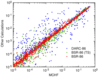
Figure 1: Comparison of $f$-values (dimensionless) from the structure models used in the present BSR, BSR-86 (TS), and DARC-86 calculations with the MCHF results Froese-Fischer and Tachiev (2004). $x$-axis: $f$ results for a certain transition calculated with the MCHF method Froese-Fischer and Tachiev (2004); $y$-axis: $gf$ results for the same transition calculated with $\bullet$ BSR (present work), $\blacksquare$ BSR-86 (TS) Tayal and Sossah (2015) and $\blacktriangledown$ DARC-86 Aggarwal and Keenan (2017).

Figure 1 exhibits a comparison of the MCHF oscillator strengths with those from the structure calculations used in the present BSR and the previous BSR-86 (TS) models Tayal and Sossah (2015), as well as the DARC-86 calculations Aggarwal and Keenan (2017) for transitions between all 86 target levels presented in Table LABEL:tab:energies. In the absence of experimental data, we consider the MCHF calculations Froese-Fischer and Tachiev (2004) as the reference to be compared with. These data are also the recommended values in the NIST compilation Kramida et al. (2016) as the most accurate currently available structure data for the $\mathrm{Mg}^{4+}$ ion. There is very good agreement between the present results and the MCHF predictions for all transitions, including the very weak ones with small $f$-values. This suggests similarly accurate configuration mixing in both calculations. The $f$-values used in the BSR-86 (TS) model show somewhat larger deviations, mainly for the weak transitions. The GRASP results for the DARC-86 model, on the other hand, differ considerably from the MCHF values for many transitions, including even relatively strong ones with $f$-values larger than $10^{-3}$. This is a clear indication that the GRASP target wavefunctions miss important CI corrections.

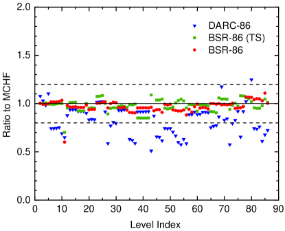
Figure 2: Lifetimes from the structure models used in the present BSR, BSR-86 (TS), and DARC-86 calculations, normalized to the MCHF predictions Froese-Fischer and Tachiev (2004). The dashed lines indicate the bands of $\pm 20\%$ deviation.

Variations in the $f$-values also lead to different predictions of the lifetimes. A comparison of the lifetimes from the various calculations is shown in Fig. 2. As expected, the present BSR lifetimes are in closest agreement with the MCHF results Froese-Fischer and Tachiev (2004). Except for the weak transition ($1-11$) to the $\mathrm{(2s^{2}\,2p^{3}(^{4}S)\,3s)^{5}S_{2}^{\rm o}}$ state, all our values agree with the MCHF results within $10\%$. The lifetimes of BSR-86 (TS) Tayal and Sossah (2015) agree within $20\%$, whereas the GRASP results of DARC-86 Aggarwal and Keenan (2017) again exhibit much larger deviations for many levels, both for low-lying and high-lying states. This indicates, once again, that the GRASP configuration expansions are far from converged. Consequently, the accuracy of the predicted collision strengths from the DARC-86 model with these inferior structure data as input are highly questionable. This will be further discussed below.

II.2 Scattering calculations

We performed two sets of scattering calculations. In the first model, BSR-86, we selected the same set of target states as in the previous BSR-86 (TS) and DARC-86 calculations. Comparison between the predictions from these three 86-state models allows us to directly draw conclusions regarding the sensitivity of the final rate coefficients to the target structure description. In our second model we additionally included the states from the $\mathrm{2s^{2}\,2p^{4}\,4}l$ and $\mathrm{2s\,2p^{5}\,3}l$ configurations, yielding 316 levels overall. This BSR-316 model allows us to check the convergence of the CC expansion, especially for transitions to higher-lying states.

The close-coupling equations were solved by means of the R-matrix method, using a parallelized version of the BSR complex Zatsarinny (2006). The distinctive feature of the method is the use of B-splines as a universal basis set to represent the scattering orbitals in the inner region of $r\leq a$. Hence, the R-matrix expansion in this region takes the form

$$\Psi_{k}(x_{1},\ldots,x_{N+1})=$$

$${\cal A}\sum_{ij}\bar{\Phi}_{i}(x_{1},\ldots,x_{N};\hat{\mathbf{r}}_{N+1}\sigma_{N+1})\,r_{N+1}^{-1}\,B_{j}(r_{N+1})\,a_{ijk}$$

$$+\sum_{i}\chi_{i}(x_{1},\ldots,x_{N+1})\,b_{ik}\,.$$ (2)

Here ${\cal A}$ denotes the antisymmetrization operator, the $\bar{\Phi}_{i}$ are the channel functions constructed from the $N$-electron target states and the angular and spin coordinates of the projectile, and the splines $B_{j}(r)$ represent the radial part of the continuum orbitals. The $\chi_{i}$ are additional $(N\!+\!1)$-electron bound states. In standard $R$-matrix calculations Burke (2011), the latter are included one configuration at a time to ensure completeness of the expansion when compensating for orthogonality constraints imposed on the continuum orbitals. The use of nonorthogonal one-electron radial functions in the BSR method, on the other hand, allows us to avoid these configurations for compensating orthogonality restrictions, thereby avoiding the pseudoresonance structure that may appear in calculations with an extensive number of bound channels $\chi_{i}$ in the CC expansion.

In the inner region, we used the same B-spline set as for the target description described above. The maximum interval in the B-spline grid was $0.25\,a_{0}$. This is sufficient to cover electron scattering energies up to $50\,\mathrm{Ry}$. Numerical calculations were performed for 60 partial waves, with total electronic angular momentum $J=1/2-59/2$, for both even and odd parities. In the BSR-86 model, the maximum number of channels in a single partial wave was $388$ while it was $1568$ in BSR-316. With a basis size of 82 B-splines, this required the diagonalization of matrices with dimensions up to about $32\,000$ and $130\,000$, respectively. The former calculations could still be performed on modern desktop machines, while the latter were carried out with parallelized versions of the BSR complex, using supercomputers with distributed memory.

For the outer region we employed the parallel version of the PSTGF program (http://www.apap-network.org/codes.html). In the resonance region for impact energies below the excitation energy of the highest level included in the CC expansion, we used a fine energy step of $10^{-5}\,z^{2}\,\mathrm{Ry}$, with $z=4$ as the target ionic charge, to properly map those resonances. For energies above the highest excitation threshold included in the CC expansion, the collision strengths vary smoothly, and hence we chose a coarser step of $10^{-2}\,z^{2}\,\mathrm{Ry}$. Altogether, $51416$ energies for the colliding electron were considered in the BSR-86 model and $71376$ energies in the BSR-316 model. We calculated collision strengths up to $50\,\mathrm{Ry}$, which is about five times the ionization potential of $\mathrm{Mg}^{4+}$. For even higher energies, if needed, we extrapolated $\Omega$ using the well-known asymptotic energy dependence of the various transitions. To obtain effective collision strengths $\Upsilon(T_{\mathrm{e}})$, we convoluted $\Omega$ with a Maxwellian distribution for an electron temperature $T_{\mathrm{e}}$, i.e.,

$$\Upsilon_{i-j}(T_{\mathrm{e}})\ =\ \int_{E_{th}}^{\infty}{\rm d}E\,\Omega_{i-j}(E)\,\exp\left(\frac{E-E_{th}}{kT_{\mathrm{e}}}\right)\,.$$ (3)

Here $E_{th}$ is the $i-j$ transition energy and $k$ is the Boltzmann constant. We calculated $\Upsilon$ for temperatures between $10^{3}$ and $10^{6}\,\mathrm{K}$. The entire table with effective collision strengths for all temperatures and transitions included in the BSR-316 model can be found online in the Supplemental Material provided with the present manuscript.

III Results and Discussion

III.1 BSR-86 calculations

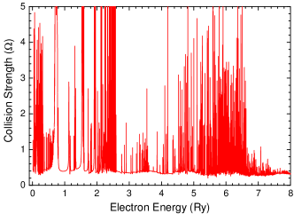
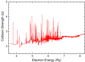
Figure 3: Collision strength $\Omega$ (dimensionless) for electron-impact excitation of the $1-2$ $\mathrm{(2s^{2}\,2p^{4}\,{}^{3}P_{2}-2s^{2}\,2p^{4}\,{}^{3}P_{1})}$ (top) and $4-9$ $\mathrm{(2s^{2}\,2p^{4}\,{}^{1}D_{2}-2s\,2p^{5}\,{}^{1}P_{1}^{\mathrm{o}})}$ (bottom) transitions in $\mathrm{Mg}^{4+}$, as obtained in the present BSR-86 model.

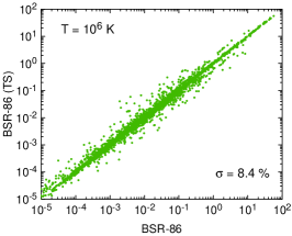
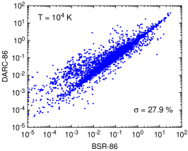
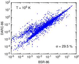
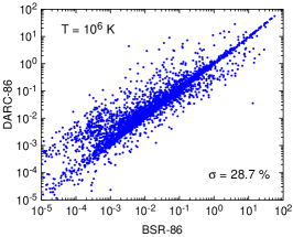
Figure 4: Comparison of effective collision strengths $\Upsilon$ (dimensionless) obtained in the present BSR-86 model with BSR-86 (TS) (upper panels), DARC-86 (middle panels), and RM-37 (lower panels) for three temperatures. Also indicated in the panels is the average deviation $\sigma$ from the BSR-86 results. $x$-axis: $\Upsilon$ results for a certain transition calculated with present BSR-86 model; $y$-axis: $\Upsilon$ results for the same transition calculated with other previous model.

As our first example, Fig. 3 exhibits the resonance structure of the collision strength $\Omega$ for the forbidden M1 transition $\mathrm{(2s^{2}\,2p^{4}\,{}^{3}P_{2}-2s^{2}\,2p^{4}\,{}^{3}P_{1})}$ and for the dipole-allowed transition $\mathrm{(2s^{2}\,2p^{4}\,{}^{1}D_{2}-2s\,2p^{5}\,{}^{1}P_{1}^{\mathrm{o}})}$. We see the typical resonance structure for electron$-$ion scattering that consists of numerous closed-channel resonances, most of which are narrow. This resonance structure provides the dominant part of the collision strength for weak forbidden transitions, but it only yields a relatively small contribution to strong dipole-allowed transitions. Visual comparison with similar plots from the DARC-86 calculation Aggarwal and Keenan (2017) shows good qualitative agreement between the calculations for these two cases. This also indicates that both calculations sufficiently resolve the rich structure. Hence, further increasing the number of energy points would not lead to noticeable corrections.

A global comparison between the present BSR-86 results and the effective collision strengths obtained previously is presented in Fig. 4 at three different temperatures. The best agreement is observed with the BSR-86 (TS) predictions Tayal and Sossah (2015). The average relative deviation is around $8\%$, which is considered a very good agreement for such type of calculation. Much worse agreement (with average deviations of almost $30\%$) is observed with the DARC-86 calculations Aggarwal and Keenan (2017). To some extent the dispersions at all three temperatures are similar to the ones seen for the $f$-values in Fig. 1. This is a clear indication that the target structure description is the principal source for the differences. For completeness, Fig. 4 also contains a comparison with the earlier RM-37 results Hudson et al. (2009). In addition to only coupling the lowest 37 levels of $\mathrm{Mg}^{4+}$, the energy mesh used in the RM-37 calculation is much coarser than in the other calculations. This may lead to a poor account of the resonance contributions. As discussed below, some of the RM-37 collision strengths exhibit apparent pseudoresonance structure. As a result, the average deviation of $44\%$ from the present results is understandable.

As shown by the above comparison, our present work confirms the validity of previous BSR-86 (TS) results Tayal and Sossah (2015). The differences are reasonable and can be explained by the different structure descriptions. This conclusion contradicts the statements of Aggarwal and Keenan Aggarwal and Keenan (2017), who declared that the BSR-86 (TS) results are incorrect and assessed the corresponding $\Upsilon$-values as unreliable. They also expressed doubts about the ability of the BSR approach to avoid pseudoresonances, and thereby to generate accurate results in general.

The principal argument of Aggarwal and Keenan Aggarwal and Keenan (2017) is that the BSR $\Upsilon$-values show a big “hump” at $10^{5}\,\mathrm{K}$ for almost all transitions to the state #86, and that the collision strengths appear to be very much underestimated at low(er) temperatures. Such a dependence of $\Upsilon$ looks unphysical and hence the appearance of pseudoresonances in the BSR-86 (TS) calculation was suggested. Since the suspicion of Aggarwal and Keenan regarding the correctness of the results for state #86 appears to be warranted, we decided to perform a detailed analysis and requested the original values for the collision strength $\Omega$ from the authors of Tayal and Sossah (2015). We found that the dense energy mesh in the BSR-86 (TS) calculations ends right below the threshold of this last state and that there is a relatively large gap of $0.02\,\mathrm{Ry}$ between the excitation threshold and the next energy point. As a result, the corresponding near-threshold portion of the excitation function is not accounted for properly when calculating $\Upsilon$ for this state. This finding explains the observations of Aggarwal and Keenan, but the problem is actually limited to transitions to state #86. A similar analysis for other states of $\mathrm{Mg}^{4+}$ does not confirm the conclusions of Aggarwal and Keenan. The extrapolation of their conclusions from a single level to all others is simply not warranted.

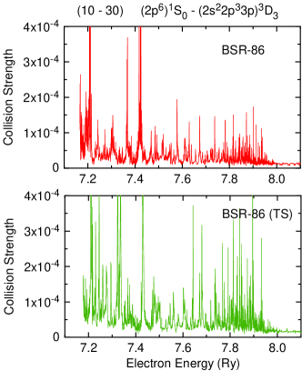
Figure 5: Collision strength $\Omega$ for electron-impact excitation of the $10-30$ transition in the BSR-86 (top) and BSR-86 (TS) (bottom) models.

Also, the suggested appearance of pseudoresonances in the BSR calculations contradicts the findings of Aggarwal and Keenan Aggarwal and Keenan (2017) that for many transitions (especially from levels below #12) the DARC $\Upsilon$-values are still much larger, up to two orders of magnitude. The reason given is the large difference in the background collision strengths. One such example is the $10-30$ ($\mathrm{2p^{6}\,{}^{1}S_{0}-2s^{2}\,2p^{3}\,3p\,^{3}D_{3}}$) transition, for which Aggarwal and Keenan exhibit the collision strength in Fig. 6 of Aggarwal and Keenan (2017). The BSR collision strength for this transition is shown in Fig. 5. We see close agreement between the BSR-86 and BSR-86 (TS) results. Visual comparison with the DARC-86 predictions reveals drastic deviations in both shape and magnitude. Whereas the BSR calculations exhibit the typical resonance structure consisting of dense but narrow resonances, the DARC cross section is dominated by three intense and broad maxima, which are typical for pseudoresonances. In other words, we arrive at the opposite conclusion compared to Aggarwal and Keenan regarding the possible effect of pseudoresonances on the results. It is also worth noting that the $10-30$ transition is a strongly forbidden three-electron-jump M3 transition whose strength depends strongly on the correlation corrections in the underlying target description as well as close-coupling effects.

III.2 BSR-316 calculations

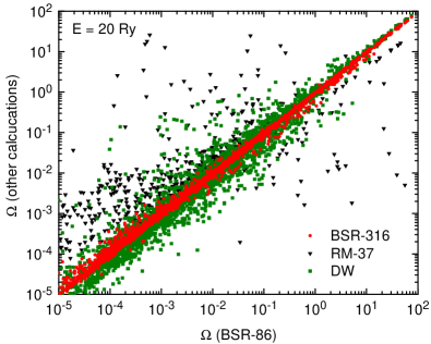
Figure 6: Comparison of collision strengths for the BSR-86 model with the DW, RM-37, and BSR-316 calculations at the electron energy $E=20\,\mathrm{Ry}$. $x$-axis: $\Omega$ results for a certain transition calculated with present BSR-86 model; $y$-axis: $\Omega$ results for the same transition calculated with $\bullet$ present BSR-316 model, $\blacktriangledown$ RM-37 Hudson et al. (2009), $\blacksquare$ DW Bhatia et al. (2006).

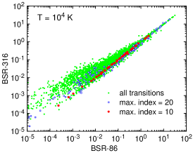
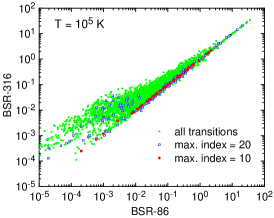
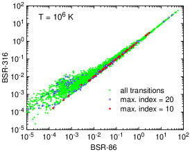
Figure 7: Comparison of effective collision strengths obtained in the present BSR-86 and BSR-316 models. In addition to all transitions, we illustrate the situation for the lowest 10 and 20 states, respectively. $x$-axis: $\Upsilon$ results for a certain transition calculated with BSR-86 model; $y$-axis: $\Upsilon$ results for the same transition calculated with BSR-316 model.

Figure 6 exhibits the collision strengths for different models at the electron energy of $E=20\,\mathrm{Ry}$, i.e., above the resonance region. This allows us to compare the background collision strengths. We found close agreement between the BSR-86 and BSR-316 background $\Omega$ for the majority of transitions. The differences with the distorted-wave (DW) results of Bhatia et al. (2006) reflect the close-coupling effects and, once again, the different target descriptions. Somewhat surprisingly, however, we notice much larger discrepancies with the RM-37 than with the DW results, even though the former model includes close-coupling and employs relatively accurate target wavefunctions. Such large deviations of the RM-37 collision strengths from both the BSR-86 and DW results again suggests the presence of pseudoresonances for some transitions. This conclusion is supported when plotting the RM-37 data presented in their online tables. For the problematic transitions, i.e., those far away from the diagonal line in Fig. 6, the RM-37 collision strengths exhibit an unphysical energy dependence, with broad resonances at higher energies. This is indeed a typical situation for R-matrix calculations with the standard Belfast codes, unless special care is taken to avoid these pseudoresonances, as outlined by Gorczyca and Badnell (1997).

In fact, the lack of balance between the $N$-electron (target) plus projectile scattering part and the $(N+1)$-electron pure bound part of the CC expansion (II.2) may also have caused the appearance of pseudoresonance structure in the DARC-86 calculations. Their target CI expansions and the $(N+1)$-electron $\chi_{i}$ functions contain configurations with a 2s hole, whereas no scattering channels with excitations out of the 2s subshell were included. This may have led to an overestimate of the 2s resonance contribution.

Figure 7 presents a comparison of effective collision strengths from the present BSR-86 and BSR-316 models. As expected, the corrections for the strong transitions are small and the corresponding rates are expected to be converged. The rate coefficients for all transitions between the lowest 10 levels with configurations $\mathrm{2s^{2}\,2p^{4}}$, $\mathrm{2s\,2p^{5}}$, and $\mathrm{2p^{6}}$ are stable against changes in the size of the CC expansion, for both strong dipole and weak intercombination transitions.

However, some transitions to the first excited $\mathrm{2s^{2}\,2p^{3}\,3}l$ states already exhibit noticeable changes in their effective collision strengths. There is a typical enhancement due to additional resonances, which was previously pointed out by Fernández-Menchero et al. for $\mathrm{Fe^{20+}}$ Fernández-Menchero et al. (2016). A more detailed analysis shows that the most dramatic changes occur for the weak two- and three-electron transitions from the $\mathrm{2s\,2p^{5}}$ and $\mathrm{2p^{6}}$ levels to the $\mathrm{2s^{2}\,2p^{3}\,3}l$ states. In these cases, the enhancement of the collision rates is not only due to additional resonance structure but also due to changes (mainly enhancement) of the background collision strengths. The resonance structure for these transitions also changes dramatically due to the inclusion of the $\mathrm{2s\,2p^{3}\,3}l$ target states that lead to the appearance of strong resonances with configurations $\mathrm{2s\,2p^{3}}\,3l\,3l^{\prime}$.

IV Summary and conclusions

In response to recent criticism of the BSR method, and in order to resolve the reasons for the large discrepancies between existing datasets, we have presented new extensive calculations of the oscillator strengths and effective collision strengths for the $\mathrm{Mg}^{4+}$ ion. Significant attention was devoted to the uncertainties in the scattering data due to the target structure description and the size of the close-coupling expansion. Our detailed and comprehensive comparison of the existing datasets allows us to draw conclusions about their likely accuracy.

First, we independently obtained electron-impact excitation collision strengths for the $\mathrm{Mg}^{4+}$ ion with the same number of target states in the close-coupling expansion as in the recent DARC-86 and BSR-86 (TS) calculations. Comparing the results directly reveals the influence of the different structure descriptions. The good agreement between our oscillator strengths with those from extensive MCHF calculations indicates that our target structure description is the most accurate used so far. The significant differences in the collision strengths seen with the DARC-86 results in many cases suggest that the target structure is the main source of inaccuracy and uncertainty in these calculations, with the largest effects on transitions involving highly excited levels. There are also indications of a remaining pseudoresonance structure in the DARC-86 calculations.

On the other hand, we obtained very reasonable agreement with the results from the previous BSR-86 (TS) calculation Tayal and Sossah (2015), except for excitation of the very last level (#86) at low temperatures. For this particular state, the deviations could simply be explained by too coarse of an energy grid in the near-threshold region of the BSR-86 (TS) calculation. Our findings, therefore, contradict the conclusions of Aggarwal and Keenan Aggarwal and Keenan (2017) regarding a general inaccuracy of the BSR-86 (TS) results. Rather than concentrating on comparing collision strengths for a single level (for which we explained the apparent problem), our conclusions are based on a comprehensive comparison for all transitions.

We also compared the present results with other available datasets. Overall good agreement was obtained with the DW collision strengths of Bhatia et al. (2006) at electron energies above the resonance region. The noticeable difference for some transitions is again connected with the too limited CI expansions in the DW calculations. The largest discrepancies were seen with the RM-37 results Hudson et al. (2009). The latter calculations are likely the least accurate due to several reasons, including a still possibly insufficient quality of the target description, a smaller CC expansion, and the indication of pseudoresonances.

Finally, we carried out much more extensive BSR-316 calculations, which additionally included the $\mathrm{2s^{2}\,2p^{4}\,4}l$ and $\mathrm{2s\,2p^{5}\,3}l$ target states. This led to the appearance of new resonances. Also, significant corrections were revealed for transitions to high-lying states and between closely-spaced levels. Due to the superior target structure generated in the present work and the larger CC expansions, we believe that the present results are the currently best for electron-impact excitation of $\mathrm{Mg}^{4+}$. The differences between the BSR-86 and the BSR-316 results may in fact serve as an uncertainty estimate for the available excitation rates. Our final table contains the radiative and collision parameters for transitions between all 316 target states. We are most confident regarding the accuracy of the collision strengths between the first 86 states presented in Table LABEL:tab:energies. The higher-lying states were included mainly to check the convergence of the results. Improving the accuracy of the collision strengths for these states would require even larger calculations whose computational demands are beyond currently available resources.

References

- Hudson et al. (2009) C. E. Hudson, C. A. Ramsbottom, P. H. Norrington, and M. P. Scott, Astron. Astroph. 494, 729 (2009).
- Tayal and Sossah (2015) S. S. Tayal and A. M. Sossah, Astron. Astroph. 574, A87 (2015).
- Aggarwal and Keenan (2017) K. M. Aggarwal and F. P. Keenan, Can. J. Phys. 95, 9 (2017).
- Hibbert (1975) A. Hibbert, Comp. Phys. Comm. 9, 141 (1975).
- Berrington et al. (1995) K. A. Berrington, W. B. Eissner, and P. H. Norrington, Comp. Phys. Comm. 92, 290 (1995).
- Griffin et al. (1998) D. C. Griffin, N. R. Badnell, and M. S. Pindzola, J. Phys. B: At. Mol. Opt. Phys. 31, 3713 (1998).
- Froese-Fischer et al. (2007) C. Froese-Fischer, G. Tachiev, G. Gaigalas, and M. R. Godefroid, Comp. Phys. Comm. 176, 559 (2007).
- Zatsarinny and Bartschat (2013) O. Zatsarinny and K. Bartschat, J. Phys. B: At. Mol. Opt. Phys. 46, 112001 (2013).
- Zatsarinny (2006) O. Zatsarinny, Comp. Phys. Comm. 174, 273 (2006).
- Hudson and Bell (2006) C. E. Hudson and K. L. Bell, Astron. Astroph. 452, 1113 (2006).
- Editors (2011) Editors, Phys. Rev. A 83, 040001 (2011).
- Chung et al. (2016) H.-K. Chung, B. J. Braams, K. Bartschat, A. G. Császár, G. W. F. Drake, T. Kirchner, V. Kokoouline, and J. Tennyson, J. Phys. D: Appl. Phys. 49, 363002 (2016).
- Mazzotta et al. (1998) P. Mazzotta, G. Mazzitelli, S. Colafrancesco, and N. Vittorio, Astron. Astroph. Suppl. Ser. 133, 403 (1998).
- Zatsarinny and Froese-Fischer (2009) O. Zatsarinny and C. Froese-Fischer, Comp. Phys. Comm. 180, 2041 (2009).
- Kramida et al. (2016) A. Kramida, Yu. Ralchenko, J. Reader, and and NIST ASD Team, NIST Atomic Spectra Database (ver. 5.4), [Online]. Available: http://physics.nist.gov/asd [2016, September 30]. National Institute of Standards and Technology, Gaithersburg, MD. (2016).
- Froese-Fischer and Tachiev (2004) C. Froese-Fischer and G. Tachiev, At. Data Nucl. Data Tables 87, 1 (2004).
- Burke (2011) P. G. Burke, -Matrix of Atomic Collisions: Application to Atomic, Molecular, and Optical Processes (Springer-Verlag, New-York, 2011).
- Bhatia et al. (2006) A. K. Bhatia, E. Landi, and W. Eissner, At. Data Nucl. Data Tables 92, 105 (2006).
- Gorczyca and Badnell (1997) T. W. Gorczyca and N. R. Badnell, J. Phys. B: At. Mol. Opt. Phys. 30, 3897 (1997).
- Fernández-Menchero et al. (2016) L. Fernández-Menchero, A. S. Giunta, G. Del Zanna, and N. R. Badnell, J. Phys. B: At. Mol. Opt. Phys. 49, 085203 (2016).