TOWARDS EXASCALE REAL-TIME RFI MITIGATION

Abstract

We describe the design and implementation of an extremely scalable real-time RFI mitigation method, based on the offline AOFlagger. All algorithms scale linearly in the number of samples. We describe how we implemented the flagger in the LOFAR real-time pipeline, on both CPUs and GPUs. Additionally, we introduce a novel simple history-based flagger that helps reduce the impact of our small window on the data.

By examining an observation of a known pulsar, we demonstrate that our flagger can achieve much higher quality than a simple thresholder, even when running in real time, on a distributed system. The flagger works on visibility data, but also on raw voltages, and beam formed data. The algorithms are scale-invariant, and work on microsecond to second time scales. We are currently implementing a prototype for the time domain pipeline of the SKA central signal processor.

Index Terms—  RFI, real-time, LOFAR, SKA, CSP, TDT

1 Introduction

Radio Frequency Interference (RFI) mitigation is extremely important to take advantage of the vastly improved bandwidth, sensitivity, and field-of-view of exascale telescopes. For current instruments, RFI mitigation is typically done offline, and in some cases (partially) manually. At the same time, it is clear that due to the high bandwidth requirements, RFI mitigation will have to be done automatically, and in real-time, for exascale instruments.

In general, real-time RFI mitigation will be less precise than offline approaches. Due to memory constraints, there is much less data to work with, typically only in the order of one second or less, as opposed to the entire observation. In addition, due to memory limitations and the fact that processing is typically done in a distributed system, we can record only limited statistics of the past. Moreover, we will typically have only few frequency channels locally available at each compute node. Finally, the amount of processing that can be spent on RFI mitigation is extremely limited due to computing constraints and a limited power budget. Many existing algorithms are therefore far too expensive and not applicable.

Nevertheless, there are many potential benefits as well, which include the possibility of working on higher time and frequency resolutions, before any integration is done, leading to more accurate results. Most importantly, we can remove RFI before beam forming, which combines data from all receivers. With beam forming, not only the signals, but also the RFI that is present in the data streams from the separate receivers is combined, effectively taking the union of all RFI. Thus, the RFI from any receiver will pollute all beams. Therefore, it is essential to also perform real-time RFI mitigation before the beam former, even though the data rates can be very high at this point. This is particularly important for pulsar surveys, for instance.

The algorithms we use are based on earlier work by Offringa and others [1, 2, 3]. Although our techniques are generic, we describe how we implemented real-time RFI mitigation for one of the SKA pathfinders: The Low Frequency Array (LOFAR) [4]. The modified RFI mitigation algorithms we introduce here are extremely fast, and the computational requirements scale linearly in the number of samples and frequency channels. We evaluate the quality of the algorithms with LOFAR pulsar observations. Using the signal-to-noise ratios of the folded pulse profiles, we can qualitatively and quantitatively compare the impact of different real-time RFI mitigation algorithms.

In addition to CPU versions, we have developed a prototype for Graphical Processing Units (GPUs). We present the very promising performance results of performing real-time RFI mitigation on GPUs. Finally, we are now working on incorporating our CPU and GPU codes in the SKA Central Signal Processor (CSP), in the context of the Time Domain Team (TDT) pulsar and transient pipeline.

2 LOF: THE LOFAR ONLINE FLAGGER

For the offline RFI mitigation for the LOFAR telescope, we use the AOFlagger [3]. This flagger is relatively efficient, and is fast enough to be applied in modern high-resolution observatories. The AOFlagger operates on visibility data, and currently is used only in the imaging mode. Although the AOFlagger provides a selection of many different algorithms, for online use, we ported the most important and successful ones to the LOFAR real-time central processing system, that originally ran on an IBM Blue Gene/p supercomputer. We also ported the algorithms to NVIDIA GPUs using CUDA, as described in Section 6.1. We call our implementation of the real-time flagger “LOF”, short for LOFAR Online Flagger.

2.1 The SumThreshold algorithm

The most important algorithm we use is SumThreshold [1]. It performs thresholding with an exponentially increasing window size, and an increasingly sharper threshold. This way, it can detect RFI at different scales. As we will demonstrate in Section 5, this indeed works well in practice, and effectively removes RFI from microsecond to multiple second scales. With SumThreshold, we define the threshold for the current window as follows:
$threshold_{I}=median+stddev*factor_{I}*sensitivity$
Where the factor is: $factor_{I}=\frac{startThreshold*p^{2}log(I)}{I}$

Typical values are p = 1.5, and sensitivity = 1.0. All measurements use the defaults, since we empirically found that they provide optimal results. No tuning is required. Figure 1 shows the threshold for different iterations.

Fig. 1: Left graphs shows the default $factor_{I}$ for different iterations; right graph shows the operation of SumThreshold. The sliding window doubles every iteration.

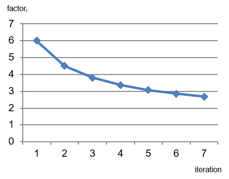
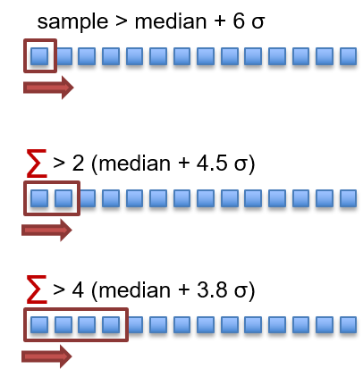
Figure 1 shows the operation of the SumThreshold algorithm. With the default values, the algorithm begins the first iteration as a simple thresholder, flagging all single samples that are more than 6 sigma away from the median. The second iteration doubles the window size to two samples, but lowers the threshold to 4.5 sigma. We typically run 7-10 iterations, depending on the resolution and size of the input.

SumThreshold can be run in a one-dimensional mode, as shown in Figure 1. This can then be done in both time and frequency directions. Alternatively, the algorithm can operate on 2D data in one pass as well (not shown in Figure 1). As we will explain in Section 4, for real-time use, we did implement a 2D code, but we will mostly use the one dimensional version of the algorithm for performance reasons. It is important to note that the computational complexity of the SumThreshold algorithm itself is linear in the number of samples. Therefore, the algorithm is suitable for real-time use, where we are limited by the number of compute cycles we can spend.

2.2 The scale-invariant rank operator

Fig. 2: Result of running the SIR operator. Purple samples are flagged by SumThreshold; yellow samples are subsequently flagged by the SIR operator. Image courtesy Andre Offringa.

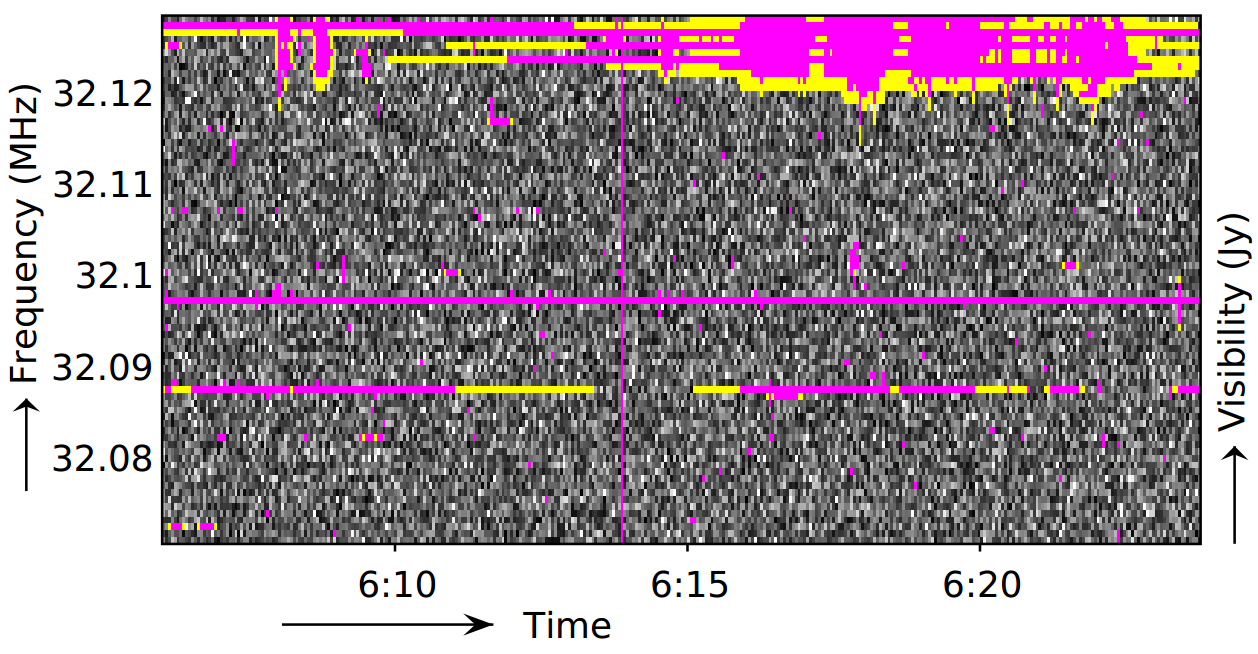
The scale-invariant rank operator [2] makes SumThreshold more robust, by extending the ranges of flagged samples by a percentage of the size of the flagged range. A typical percentage we used is 20%. This means that all ranges of consecutive flagged samples are extended by flagging 20% more samples, before and after the original range. The algorithm can be run in both the time direction and the frequency direction. The SIR operator helps to remove RFI that slowly rises and decreases in strength, that may be otherwise undetected. The result of the SIR operator is shown in Figure 2.

We use a version of the SIR operator implementation that has a linear computational complexity in the number of samples (the original implementation in the AOFlagger had worse computational complexity). The linear version of the algorithm is described in [2]. Since SIR operates on the flag masks only, and not on the actual data itself, it is extremely efficient.

3 INTEGRATION IN REAL-TIME PIPELINES

Fig. 3: The LOFAR real-time pipelines. Input data rates vary between 400 gbit/s and 1.6 tbit/s for the pre-correlation flagger, depending on the mode (4, 8 or 16 bit samples).

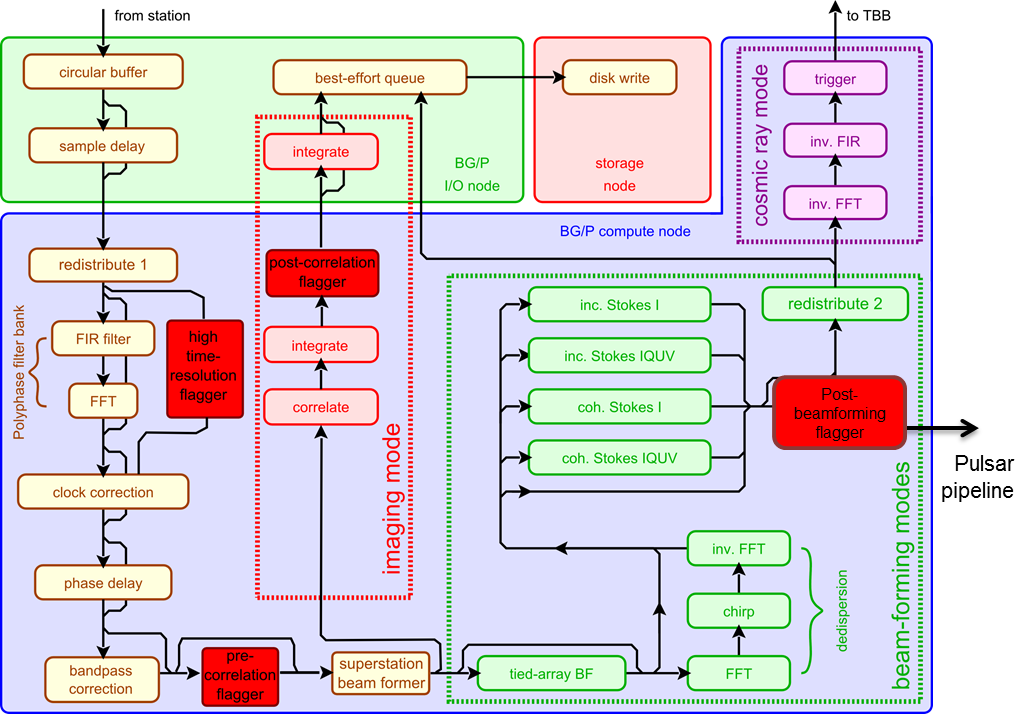
Figure 3 shows a high-level overview of the LOFAR real-time central signal processing pipeline. The entire pipeline is implemented in software, and is described in detail in [4], including a detailed performance analysis. The LOFAR online flagger components are placed in four different places in the pipeline. Depending on the configuration and the observation type, one or more different flaggers are used.

Data arrives in the form of raw voltages at the top left of the figure. Next, a number of steps are executed independently of whether we are in imaging or beam forming mode. The most important step is a polyphase filter bank that splits the broad input subbands in narrower frequency channels. Typical channel bandwidths are between 0.8 kHz and 12 kHz, with sample rates between 82 microseconds and 1.3 milliseconds. When we need extremely high time resolution (e.g, for millisecond pulsars or for the cosmic ray pipeline), we bypass the polyphase filter bank altogether. For this case we created a special high time resolution flagger.

Next, the band pass of the first polyphase filter bank that runs inside the stations on FPGAs is corrected. After this bandpass correction, we inserted our pre-correlation flagger that works on the channelized raw voltage data. It is important to do this after the band pass correction, as this ensures that the sensitivity is equal across all channels. The pre-correlation version is the most important real-time flagger, especially for the beam forming modes. The beam former does a weighted addition of the data streams from the different stations, essentially taking the union of all RFI from all stations. If RFI is present at a station, this will pollute all output beams. Especially for uncorrelated RFI and long baselines, this is sub optimal.

In addition, we can use our real-time flagger after the correlator, for real-time image-based transient detection, for example. The drawback of performing RFI mitigation after the correlator is that, depending on the number of baselines and the integration time, data rates can be higher than before the correlator. Finally, we have a post beam forming flagger that can potentially benefit from a better interference-to-noise ratio (INR). Moreover, depending on the number of output beams, this typically runs on lower data rates.

4 CHANGES FOR REAL-TIME USE

To make sure the algorithms used in the AOFlagger work in a real-time context, we had to make several changes. First, depending on the input data type of the flagger, we may have to compute amplitudes first. This is the case for the high-time resolution flagger, and for the pre-correlation flagger. The post-correlation flagger runs on visibility data directly, while the post-beam forming flagger runs on Stokes I data.

Fig. 4: Integration in the time direction to perform flagging in the frequency direction with high INR.

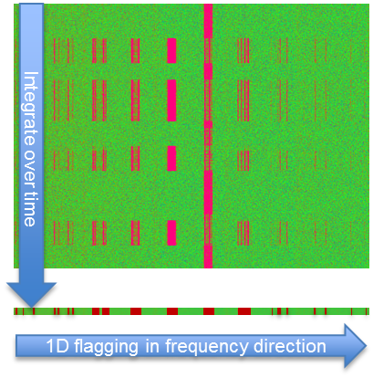
In pre-correlation mode, we typically integrate the data. We found it particularly useful to integrate the time direction fully for frequency flagging, and to integrate the frequency direction fully for time domain flagging. Figure 4 shows this. This approach has two benefits: it improves the INR, while at the same time reducing the computational costs. We first flag in the frequency direction. This removes strong narrow-band RFI that would otherwise decrease the quality of the statistics used to compute the thresholds. We found that this is frequently present in the LOFAR RFI environment. This also is the reason we create the narrow approximately 1kHz channels. We have an alternative method that implements 2D flagging, while partially integrating in one or both dimensions to improve INR and to reduce compute costs.

All flaggers have linear computational complexity in the number of samples, regardless of their place in the real-time pipeline. For instance, the pre-correlation flagger has a complexity of O(nrStations * nrPolarizations * nrChannels * nrTimes), the post-correlation flagger is O(nrBaselines * nrPolarizations * nrChannels), and the post beam forming flagger is O(nrBeams * nrChannels * nrTimes).

4.1 Using historical information

One of the most difficult problems with real-time RFI mitigation is the very limited window on the observation. Typically, we can only keep one second of data or less (e.g., a tenth of a second) in memory. Similarly, we can only keep a very limited number of frequency channels in memory. This is due to memory constraints, and partially because we process the data on a distributed system. We create parallelism by performing domain decomposition. This typically means that different frequency subbands are processed on different compute nodes. Finally, in some cases, processing a second of input data takes longer than a second. To still meet the real-time requirements, subsequent seconds are processed partially overlapping in time, by different compute nodes. All these factors severely limit our situational awareness.

Our solution for this problem is the introduction of a novel history flagger that performs simple thresholding of the current data chunk, based on statistics of past chunks. Pseudo code for this history flagger is shown below.

⬇

// For all channels, we do the following:

// Keep a history buffer (sliding window) of

// means of unflagged samples of the past seconds

currentValue = meanOfUnflaggedSamples()

historyMean = meanOfMeans()

historyStddev = stddevOfMeans()

threshold= historyMean + sensitivity * historyStddev

if(currentValue < threshold) {

addToHistory(station, subband, currentValue)

} else {

addToHistory(station, subband, threshold)

flagThisIntegrationTime()

}

Fig. 5: The history buffer.

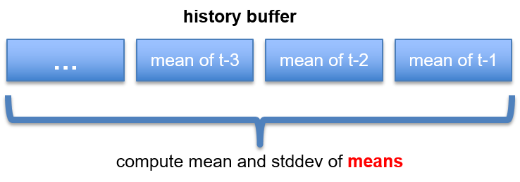
As shown in Figure 5, our flagger uses a history buffer that stores the means of the unflagged samples of the previous seconds of data. This buffer essentially is a sliding window over the data. We use the buffer to compute the mean and standard deviation of the previous seconds, to give us a frame of reference for the overall signal strength of the current second. This is especially important, since a strong broadband RFI event that lasts longer than our integration time can otherwise not be detected.

4.2 Statistics in a real-time pipeline

The quality of the statistics that we compute and keep is important, especially since the window on the data is so small. We use only very basic statistics, such as (winsorized) means, medians, standard deviations, and the MAD (Median Absolute Deviation). To compute the medians, which can be expensive, we use an efficient O(N) implementation (note that sorting the data already is O(NlogN) at best. More complications result from using a distributed platform: statistics are often in the wrong place, at the wrong time. Moreover, we cannot compute running statistics, since a second of data takes more than a second to compute. Finally, our real-time pipeline uses complex communication patterns due to scheduling, and asynchronous communication for better performance. Together, this means that even computing basic statistics is quite complex in practice.

An important consideration for the history flagger is presented by the space requirements of the statistics of the past we want to keep in the history buffer. Let us use LOFAR numbers as an example. For the pre-correlation flagger, we need $stations*subbands*channels*32bits=64*248*256*4$ = 15.5 MByte per second. If we want to keep 5 minutes of history in the buffer, we already need 300 samples, leading to a storage requirement of 4.5 GBytes. After the correlator, requirements are even higher: $baselines*subbands*channels*32bits=2080*248*256*4$ = 504 MByte per second, which, even if we want to store only 5 minutes, already leads to 148 Gbytes of statistics data. Therefore, in practice, even keeping these very limited statistics of only a few minutes of the past already is extremely difficult, and down-sampling may be needed.

5 evaluation

In this section, we will present a qualitative and quantitative evaluation of the real-time flagger, using a LOFAR pulsar observation. We use the pulsar pipeline, because it allows for a quantitative comparison: we perform dedispersion and folding to create a folded pulse profile. Next, we compute the SNR of the pulse profile as a measure of quality. Better RFI mitigation directly leads to a higher SNR.

5.1 A pulsar observation

We performed an observation of pulsar B1919+21, which has a period of 1.3373 s, a pulse width 0.04 s, and a dispersion measure (DM) of 12.455. We observed at 138.0–145.2 MHz (32 subbands) with 5 stations: CS005, CS006, RS205, RS406, and UK608. We deliberately chose a number of core stations, where RFI is expected to be correlated, a remote station in the Netherlands, where the RFI environment is known to be particularly bad, and an international station in the UK, to guarantee we also have uncorrelated RFI.

We used a special LOFAR mode that allowed us to store the raw UDP network packets, before the data even enters the correlator. This allows us to replay the entire real-time pipeline in an offline mode, enabling comparisons between different flagging algorithms, parameter settings and even observation modes (e.g., imaging or beam forming). For the beam forming mode that we use for the pulsar pipeline, we split the frequency subbands into 16 channels (12 KHz / 82 μs).

Fig. 6: Thresholding vs LOF, on raw voltages. Left: original data; right: difference threshold – LOF, i.e. RFI residuals that are flagged by LOF, but not by simple thresholding.

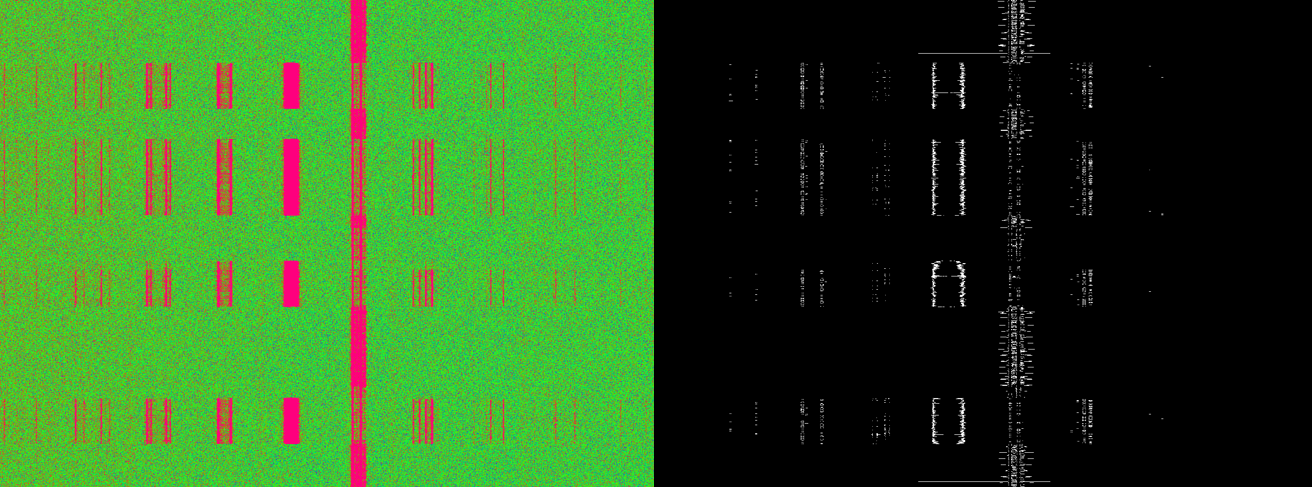
Figure 6 shows two waterfall plots. The left side is the original observation with RFI present; on the right the improvement of our LOF compared to a simple thresholding scheme, where we manually determined the optimal threshold. There clearly is a lot of residual RFI that is not removed by the thresholder, that is removed by LOF.

Fig. 7: Beam formed data (Stokes I), top panel without RFI mitigation, bottom panel with LOF.

Fig. 8: Closeup of beam formed data (Stokes I), top panel without RFI mitigation, bottom panel with LOF.

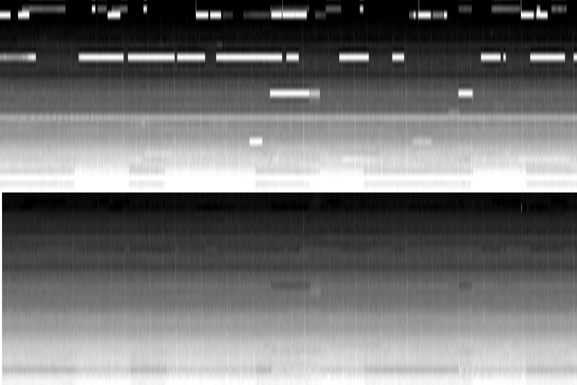
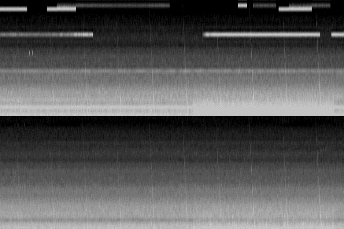
Figure 8 shows Stokes I data of an output beam; Figure 8 shows the same, but zoomed in. The top panels are without RFI mitigation, the bottom panels with LOF. Almost all RFI is removed. The data is not de-dispersed, but the pulsar signal is so strong that it is clearly visible in the data. Note that the pulses are not flagged away by our mitigation algorithms.

Fig. 9: Folded pulse profiles with and without flagging.

In Figure 9 (left side), we show the folded pulse profiles, without RFI mitigation, with a simple thresholder, and with LOF. Without RFI mitigation, the pulsar signal is completely below the noise floor, and cannot be detected. With the thresholder, the pulse is visible, but there also are false positives, caused by strong RFI events that were not removed. With LOF, there is one clear peak with the right shape, with a good SNR. This can be seen better in the right side of Figure 9, which shows the same data, but zoomed in, with the non-flagged line removed.

Fig. 10: Quality of LOF for pulsar B1919+21. LOF has significantly higher quality than simple thresholding. The quality of LOF is close to offline Presto rfifind.

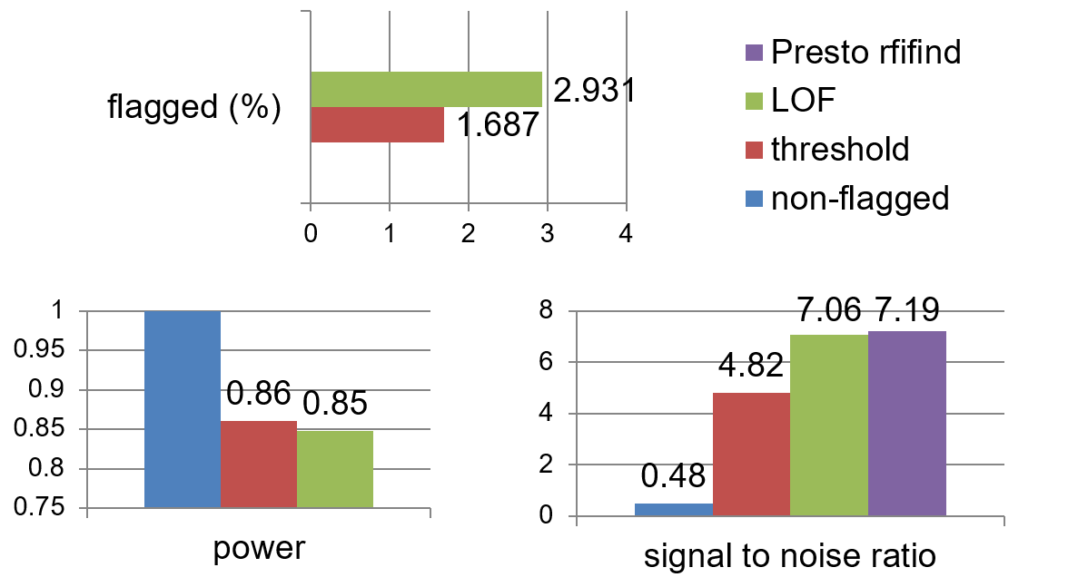
Figure 10 shows that LOF flags 2.9% of the data in the observation, significantly more than the simple thresholder that only flags 1.7%. In the bottom left graph, we show that LOF flags away about 15% of the total signal power, only slightly more than the simple thresholder. The bottom right graph shows the SNR of the folded pulse profile. LOF is significantly better than the simple thresholder, and almost as high as performing offline RFI mitigation with Presto’s rfifind [5].

6 TOWARDS EXASCALE

The LOFAR online processor needs hundreds of teraflops of computational power. Future instruments such as the Square Kilometre Array (SKA) will be much more sensitive, and will require orders of magnitude more processing [6]. Therefore, we were careful to make sure that all algorithms used in our real-time flagger have a linear computational complexity, allowing excellent scaling. In addition, we investigated the use of modern processing architectures, such as GPUs. For LOFAR, we already switched from an IBM Blue Gene/p system to a GPU cluster. For the central signal processor of the SKA, a combination of FPGAs and GPUs are likely. In this section, we present a prototype GPU version of the LOF.

6.1 GPU implementation

Fig. 11: Scalability of the GPU implementation of LOF.

With Linus Schoemaker [7], we worked on the GPU port of LOF. Due to the limited space, we will only describe the most important differences with the normal parallel CPU version here. The normal LOF exploits parallelism by scheduling different subbands to different compute nodes. Inside the compute nodes we use C++ and OpenMP for multi-threading, and asynchronous MPI messages for inter-node communication. To avoid synchronization and parallelization overhead, we make the parallelism as coarse grained as possible. This means that each thread handles all data for one subband.

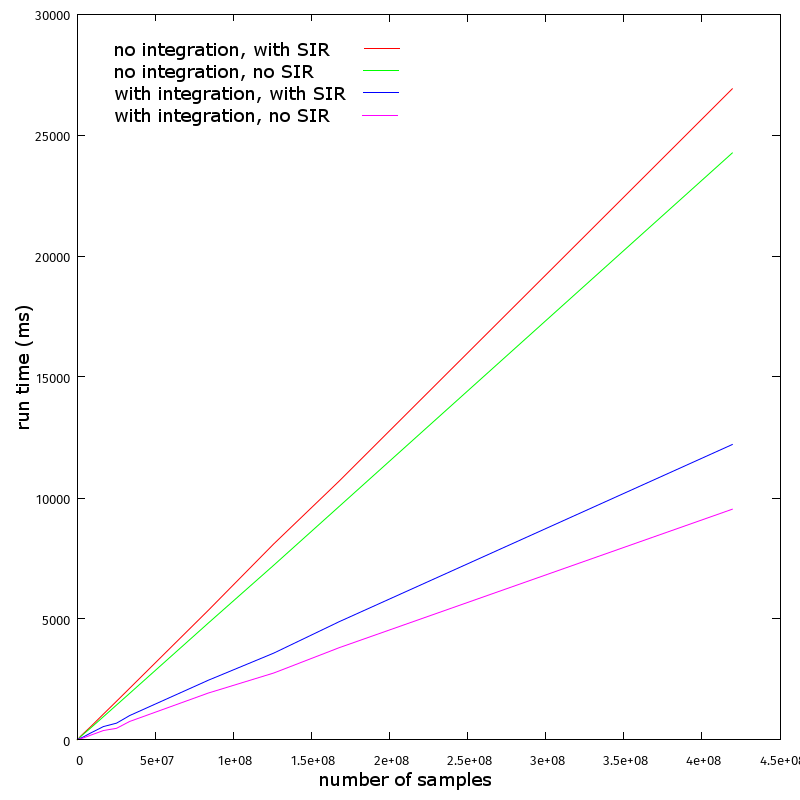
GPUs, in contrast, can efficiently exploit extremely fine grained parallelism. Hundreds of thousands of threads can work in parallel on a single GPU, without overhead. In fact, in our implementation, we create one GPU thread per sample. We exploit data-reuse by using the shared memory that is available inside the GPU’s streaming multiprocessors. The performance results are shown in figure 11. The top two lines (red and green) show the run time without doing any data integration, running SumThreshold on the full input data rate. For the red line, we also run the SIR operator; green is without. The bottom two lines show performance if we fully integrate and run SumThreshold two times, once in the frequency direction, and once in the time direction, as described in Section 4. In all cases, we achieve linear Scalability. The GPU performs so well, that we can handle all LOFAR stations on single GPU in real time.

6.2 Integration in SKA time domain pipeline

We are currently working on incorporating our CPU and GPU codes in the SKA Central Signal Processor (CSP), in the context of the Time Domain Team (TDT) pulsar and transient pipeline. The initial stages of the CSP, including the beam former, will likely use FPGAs. After the beam former, GPUs are the most likely candidate for further processing. Therefore, we will perform post-beamforming flagging using our algorithms on GPUs. For an FPGA implementation, more research is needed.

7 CONCLUSIONS AND FUTURE WORK

We have demonstrated that our online flagger can achieve much higher quality than simple thresholding, in real time, even on a distributed system. The SumThreshold algorithm was originally used mostly on visibility data. In this paper, we demonstrated that the algorithm also works well on raw voltages, pre-correlation data, and post-beam forming data. Therefore, we have one robust algorithm for extremely different scales, from microseconds to multiple seconds. The algorithms are scalable and have linear computational complexity, adding little overhead to existing pipelines. One complication is that we have an extremely limited view on our data, and therefore need a history flagger. Due to the high data rates, we have to be flexible in storage requirements, even for statistics.

We are currently working on commissioning of the GPU code for LOFAR. Moreover, we are constructing a performance model that can extrapolate Scalability towards SKA sizes. This model includes power dissipation as well, since this will be an important bottleneck for the SKA. We plan to use the Dome ExaBounds tool for this analysis [8]. All code used in this paper is available as open source:
https://github.com/NLeSC/eAstroViz.

References

- [1] A. R. Offringa, A. G. de Bruyn, and S. Zaroubi, “Post-correlation filtering techniques for off-axis source and rfi removal,” Monthly Notices of the Royal Astronomical Society, vol. 422, no. 1, pp. 563–580, 2012.
- [2] Jasper J. van de Gronde, André R. Offringa, and Jos B. T. M. Roerdink, “Efficient and robust path openings using the scale-invariant rank operator,” Journal of Math. Imaging and Vision, vol. 56, no. 3, pp. 455–471, 2016.
- [3] A.R. Offringa, A.G. de Bruyn, S. Zaroubi, and M. Biehl, “A LOFAR RFI detection pipeline and its first results,” in Proc. of Science, RFI2010, 2010, vol. II, pp. 803–806.
- [4] John W. Romein, P. Chris Broekema, Jan David Mol, and Rob V. van Nieuwpoort, “The LOFAR Correlator: Implementation and Performance Analysis,” in Proc. ACM Symposium on Principles and Practice of Parallel Programming (PPoPP’10), 2010, pp. 169–178.
- [5] S. M. Ransom, S. S. Eikenberry, and J. Middleditch, “Fourier Techniques for Very Long Astrophysical Time-Series Analysis,” The Astronomical Journal, vol. 124, pp. 1788–1809, Sept. 2002.
- [6] P. Chris Broekema, Rob V. van Nieuwpoort, and Henri E. Bal, “The square kilometre array science data processor preliminary compute platform design,” Journal of Instrumentation, July 2015.
- [7] Linus Schoemaker, “Removing Radio Frequency Interference in the LOFAR using GPUs,” M.S. thesis, VU University Amsterdam, 2015.
- [8] P. Chris Broekema, Albert-Jan Boonstra, Victoria Caparrós Cabezas, Ton Engbersen, Robert Haas, Hanno Holties, Jens Jelitto, Ronald P. Luijten, Peter Maat, Rob V. van Nieuwpoort, Ronald Nijboer, John W. Romein, and Bert Jan Offrein, “DOME: Towards the ASTRON & IBM Center for ExaScale Technology,” in Proc. ACM workshop on AstroHPC, 2012.