MULTILEVEL MAXIMUM LIKELIHOOD ESTIMATION WITH APPLICATION TO COVARIANCE MATRICES

^∗ Institute of Computer Science, Academy of Sciences of the Czech Republic
Pod Vodárenskou věží 271/2, 182 07 Praha 8, Czech Republic, and
Charles University in Prague, Faculty of Mathematics and Physics
Sokolovská 83, Prague 8, 186 75, Czech Republic
turcicova@cs.cas.cz ^† University of Colorado Denver, Denver, CO 80217-3364, USA, and
Institute of Computer Science, Academy of Sciences of the Czech Republic
Pod Vodárenskou věží 271/2, 182 07 Praha 8, Czech Republic
Jan.Mandel@ucdenver.edu ^‡ Institute of Computer Science, Academy of Sciences of the Czech Republic
Pod Vodárenskou věží 271/2, 182 07 Praha 8, Czech Republic
eben@cs.cas.cz

Key Words: hierarchical maximum likelihood; nested parameter spaces; spectral diagonal covariance model; sparse inverse covariance model; Fisher information; high dimension.

ABSTRACT

The asymptotic variance of the maximum likelihood estimate is proved to decrease when the maximization is restricted to a subspace that contains the true parameter value. Maximum likelihood estimation allows a systematic fitting of covariance models to the sample, which is important in data assimilation. The hierarchical maximum likelihood approach is applied to the spectral diagonal covariance model with different parameterizations of eigenvalue decay, and to the sparse inverse covariance model with specified parameter values on different sets of nonzero entries. It is shown computationally that using smaller sets of parameters can decrease the sampling noise in high dimension substantially.

1 INTRODUCTION

Estimation of large covariance matrices from small samples is an important problem in many fields, including spatial statistics, genomics, and ensemble filtering. One of the prominent applications is data assimilation in meteorology and oceanography, where the dimension of state vector describing the atmosphere or ocean is in order of millions or larger. Every practically available sample is a small sample in this context, since a reasonable approximation of the full covariance can be obtained only with sample size of the order of the dimension of the problem (Vershynin, 2012). In practice, the sample covariance is singular and polluted by spurious correlations. Nevertheless, it carries useful information (e.g. on covariances present in the actual atmospheric flow) and different techniques can be applied in order to improve the covariance model and its practical performance.

One common technique is shrinkage, that is, a linear combination of sample covariance and a positive definite target matrix, which prevents the covariance from being singular. The target matrix embodies some prior information about the covariance; it can be, e.g., unit diagonal or, more generally, positive diagonal (Ledoit  Wolf, 2004). See, e.g., Schäfer  Strimmer (2005) for a survey of such shrinkage approaches. Shrinkage of sample covariance towards a fixed covariance matrix based on a specific model and estimated from historical data (called background covariance) was used successfully in meteorology (Hamill  Snyder, 2000; Wang ., 2008). This approach is justified as one which combines actual (called flow-dependent) and long-term average (called climatologic) information on spatial covariances present in the 3D meteorological fields.

Another approach to improving on the sample covariance matrix is localization by suppressing long-range spurious correlations, which is commonly done by multiplying the sample covariance matrix term by term by a gradual cutoff matrix (Buehner  Charron, 2007; Furrer  Bengtsson, 2007) to suppress off-diagonal entries. The extreme case, when only the diagonal is left, is particularly advantageous in the spectral domain, as the covariance of a random field in Fourier space is diagonal if and only if the random field in cartesian geometry is second order stationary, i.e., the covariance between the values at two points depends only on their distance vector. Alternatively, diagonal covariance in a wavelet basis provides spatial variability as well (Pannekoucke ., 2007). Spectral diagonal covariance models were successfully used in operational statistical interpolation in meteorology in spherical geometry (Parrish  Derber, 1992), and versions of Ensemble Kalman Filter (EnKF) were developed which construct diagonal covariance in Fourier or wavelet space in every update step of the filter at low cost, and can operate successfully with small ensembles (Mandel ., 2010; Beezley ., 2011; Kasanický ., 2015).

Sparse covariance models, such as the spectral diagonal, allow a compromise between realistic assumptions and cheap computations. Another covariance model taking advantage of sparsity is a Gauss-Markov Random Field (GMRF), based on the fact that conditional independence of variables implies zero corresponding elements in the inverse of the covariance matrix (Rue  Held, 2005), which leads to modeling the covariance as the inverse of a sparse matrix.

However, both spectral diagonal and sparse inverse covariance models have a large number of parameters, namely all terms of the sparse matrix (up to symmetry) which are allowed to attain nonzero values. This results in overfitting and significant sampling noise for small samples. Therefore, it is of interest to reduce the number of parameters by adopting additional, problem-dependent assumptions on the true parameter values.

The principal result of this paper is the observation that if parameters are fitted as the Maximum Likelihood Estimator (MLE) and the additional assumptions are satisfied by the true parameters, then the estimate using fewer parameters is asymptotically more accurate, and often very significantly so even for small samples..

The paper is organized as follows. In Sec. 2, we provide a brief statement of MLE and its asymptotic variance. In Sec. 3, we use the theory of maximum likelihood estimation to prove that for any two nested subspaces of the parametric space containing the true parameter, the asymptotic covariance matrix of the MLE is smaller for the smaller parameter space. These results hold for a general parameter and, in the special case of MLE for covariance matrices we do not need any invertibility assumption. The applications to estimation of covariance matrices by spectral diagonal and GMRF are presented in Sec. 4, and Sec. 5 contains computational illustrations. A comparison of the performance of MLE for parametric models and of related shrinkage estimators is in Sec. 6.

2 ASYMPTOTIC VARIANCE OF THE MAXIMUM LIKELIHOOD ESTIMATOR

First, we briefly review some standard results for reference. Suppose $\mathbb{X}_{N}=\left[\bm{X}_{1},\ldots,\bm{X}_{N}\right]$ is a random sample from a distribution on $\mathbb{R}^{n}$ with density $f\left(\bm{x},\bm{\theta}\right)$ with unknown parameter vector $\bm{\theta}$ in a parameter space $\Theta\subset\mathbb{R}^{p}$. The maximum likelihood estimate $\bm{\hat{\theta}}_{N}$ of the true parameter $\bm{\theta}^{0}$ is defined by maximizing the likelihood

$$\bm{\hat{\theta}}_{N}=\arg\max_{\bm{\theta}}\mathcal{L}\left(\bm{\theta}|\mathbb{X}_{N}\right),\quad\mathcal{L}\left(\bm{\theta}|\mathbb{X}_{N}\right)=\prod\limits_{i=1}^{N}\mathcal{L}\left(\bm{\theta}|\bm{X}_{i}\right),\quad\mathcal{L}\left(\bm{\theta}|\bm{x}\right)=f\left(\bm{x},\bm{\theta}\right),$$

or, equivalently, maximizing the log likelihood

$$\bm{\hat{\theta}}_{N}=\arg\max_{\bm{\theta}}\ell\left(\bm{\theta}|\mathbb{X}_{N}\right),\quad\ell\left(\bm{\theta}|\mathbb{X}_{N}\right)=\sum\limits_{i=1}^{N}\ell\left(\bm{\theta}|\bm{X}_{i}\right),\quad\ell\left(\bm{\theta}|\bm{x}\right)=\log f\left(\bm{x},\bm{\theta}\right).$$ (1)

We adopt the usual assumptions that (i) the true parameter $\bm{\theta}^{0}$ lies in the interior of $\Theta$, (ii) the density $f$ determines the parameter $\bm{\theta}$ uniquely in the sense that $f(\bm{x},\bm{\theta}_{1})=f(\bm{x},\bm{\theta}_{2})$ a.s. if and only if $\bm{\theta}_{1}=\bm{\theta}_{2}$, and (iii) $f\left(\bm{x},\bm{\theta}\right)$ is a sufficiently smooth function of $\bm{x}$ and $\bm{\theta.}$ Then the error of the estimate is asymptotically normal,

$$\sqrt{N}(\hat{\bm{\theta}}_{N}-\bm{\theta}^{0})\xrightarrow{d}\mathcal{N}_{p}(\bm{0},Q_{\bm{\theta}^{0}}),\text{ as }N\rightarrow\infty,$$ (2)

where

$$Q_{\bm{\theta}^{0}}=J_{\bm{\theta}^{0}}^{-1},\quad J_{\bm{\theta}^{0}}=\operatorname{E}\left(\nabla_{\bm{\theta}}\ell(\bm{\theta}^{0}|\bm{X})^{\top}\nabla_{\bm{\theta}}\ell(\bm{\theta}^{0}|\bm{X})\right),\quad\bm{X}\sim f\left(\bm{x},\bm{\theta}^{0}\right).$$ (3)

The matrix $J_{\bm{\theta}^{0}}$ is called the Fisher information matrix for the parameterization $\bm{\theta}^{0}$. Here, $\bm{X}$, $\bm{x}$, and $\bm{\theta}$ are columns, while the gradient $\nabla_{\bm{\theta}}\ell$ of $\ell$ with respect to the parameter $\bm{\theta}$ is a row vector, which is compatible with the dimensioning of Jacobi matrices below. The mean value in (3) is taken with respect to $\bm{X}$, which is the only random quantity in (3). Cf., e.g., (Lehmann  Casella, 1998, Theorem 5.1) for details.

3 NESTED MAXIMUM LIKELIHOOD ESTIMATORS

Now suppose that we have an additional information that the true parameter $\bm{\theta}^{0}$ lies in a subspace of $\Theta$, which is parameterized by $k\leq p$ parameters $(\varphi_{1}$,…, $\varphi_{k})^{\top}=\bm{\varphi}$. Denote by $\nabla_{\bm{\varphi}}\bm{\theta}(\bm{\varphi})$ the $p\times k$ Jacobi matrix with entries $\frac{\partial\theta_{i}}{\partial\varphi_{j}}$. In the next theorem, we derive the asymptotic covariance of the maximum likelihood estimator for $\bm{\varphi}$,

$$\hat{\bm{\varphi}}_{N}=\arg\max_{\bm{\varphi}}\ell\left(\bm{\varphi}|\mathbb{X}_{N}\right),\quad\ell\left(\bm{\varphi}|\mathbb{X}_{N}\right)=\sum\limits_{i=1}^{N}\ell\left(\bm{\varphi}|\bm{X}_{i}\right),\quad\ell\left(\bm{\varphi}|\bm{x}\right)=\log f\left(\bm{x},\bm{\theta}\left(\bm{\varphi}\right)\right),$$ (4)

based on the asymptotic covariance of $\bm{\theta}$ in (2).

Theorem 1

Assume that the map $\bm{\varphi}\mapsto\bm{\theta}(\bm{\varphi})$ is one-to-one from $\Phi\subset\mathbb{R}^{k}$ to $\Theta$, the map $\bm{\varphi}\mapsto\bm{\theta}(\bm{\varphi})$ is continuously differentiable, $\nabla_{\bm{\varphi}}\bm{\theta}(\bm{\varphi})$ is full rank for all $\bm{\varphi}\in\Phi$, and $\bm{\theta}^{0}=\bm{\theta}(\bm{\varphi}^{0})$ with $\bm{\varphi}^{0}$ in the interior of $\Phi$. Then,

$$\sqrt{N}(\hat{\bm{\varphi}}_{N}-\bm{\varphi}^{0})\xrightarrow{d}\mathcal{N}_{k}\left(\bm{0},Q_{\bm{\varphi}^{0}}\right)\text{ as }N\rightarrow\infty,$$ (5)

where $Q_{\bm{\varphi}^{0}}=J_{\bm{\varphi}^{0}}^{-1}$, with $J_{\bm{\varphi}^{0}}$ the Fisher information matrix of the parameterization $\bm{\varphi}$ given by

$$J_{\bm{\varphi}^{0}}=\nabla_{\bm{\varphi}}\bm{\theta}(\bm{\varphi}^{0})^{\top}J_{\bm{\theta}^{0}}\nabla_{\bm{\varphi}}\bm{\theta}(\bm{\varphi}^{0}).$$ (6)

Proof. From (3) and the chain rule

$$\nabla_{\bm{\varphi}}\ell(\bm{\varphi}|\bm{X})=\nabla_{\bm{\theta}}\ell(\bm{\theta}|\bm{X})\nabla_{\bm{\varphi}}\bm{\theta}(\bm{\varphi}),$$

we have

$$J_{\bm{\varphi}^{0}} =\operatorname{E}\left(\nabla_{\bm{\varphi}}\ell(\bm{\varphi}^{0}|\bm{X})^{\top}\nabla_{\bm{\varphi}}\ell(\bm{\varphi}^{0}|\bm{X})\right)$$

$$=\nabla_{\bm{\varphi}}\bm{\theta}(\bm{\varphi}^{0})^{\top}\operatorname{E}\left(\nabla_{\bm{\theta}}\ell(\bm{\theta}^{0}|\bm{X})^{\top}\nabla_{\bm{\theta}}\ell(\bm{\theta}^{0}|\bm{X})\right)\nabla_{\bm{\varphi}}\bm{\theta}(\bm{\varphi}^{0})$$

$$=\nabla_{\bm{\varphi}}\bm{\theta}(\bm{\varphi}^{0})^{\top}J_{\bm{\theta}^{0}}\nabla_{\bm{\varphi}}\bm{\theta}(\bm{\varphi}^{0}).$$

The asymptotic distribution (5) is now (2) applied to $\bm{\varphi}$.   

When the parameter $\bm{\theta}$ is the quantity of interest in an application, it is useful to express the estimate and its variance in terms of the original parameter $\bm{\theta}$ rather than the subspace parameter $\bm{\varphi}$.

Corollary 2

Under the assumptions of Theorem 1,

$$\sqrt{N}(\bm{\theta}\left(\hat{\bm{\varphi}}_{N}\right)-\bm{\theta}^{0})\xrightarrow{d}\mathcal{N}_{p}\left(\bm{0},Q_{\bm{\theta}\left(\bm{\varphi}^{0}\right)}\right)\text{ as }N\rightarrow\infty,$$ (7)

where

$$Q_{\bm{\theta}\left(\bm{\varphi}^{0}\right)}=\nabla_{\bm{\varphi}}\bm{\theta}(\bm{\varphi}^{0})J_{\bm{\varphi}^{0}}^{-1}\nabla_{\bm{\varphi}}\bm{\theta}(\bm{\varphi}^{0})^{\top}=\nabla_{\bm{\varphi}}\bm{\theta}(\bm{\varphi}^{0})\left(\nabla_{\bm{\varphi}}\bm{\theta}(\bm{\varphi}^{0})^{\top}J_{\bm{\theta}^{0}}\nabla_{\bm{\varphi}}\bm{\theta}(\bm{\varphi}^{0})\right)^{-1}\nabla_{\bm{\varphi}}\bm{\theta}(\bm{\varphi}^{0})^{\top}.$$ (8)

Proof. The lemma follows from (5) by the delta method (Rao, 1973, p. 387), since the map $\bm{\varphi\mapsto\theta}(\bm{\varphi})$ is continuously differentiable.   

Remark 3

The matrix $Q_{\bm{\theta}\left(\bm{\varphi}^{0}\right)}$ is singular, so it cannot be written as the inverse of another matrix, but it can be understood as the inverse $J_{\bm{\theta}(\bm{\varphi}^{0})}^{-1}$ of the Fisher information matrix for $\bm{\varphi}$, embedded in the larger parameter space $\Theta$.

Suppose that $\bm{\psi}$ is another parameterization which satisfies the same assumption as $\bm{\varphi}$ in Theorem 1: the map $\bm{\psi}\mapsto\bm{\theta}(\bm{\psi})$ is one-to-one from $\Psi\subset\mathbb{R}^{m}$, $k\leq m\leq p,$ to $\Theta$, $\bm{\psi}\mapsto\bm{\theta}(\bm{\psi})$ is continuously differentiable, $\nabla_{\bm{\psi}}\bm{\theta}(\bm{\psi})$ is full rank for all $\bm{\psi}\in\Psi$, and $\bm{\theta}^{0}=\bm{\theta}(\bm{\psi}^{0})$, where $\bm{\psi}^{0}$ is in the interior of $\Psi$. Then, similarly as in (7), we have also

$$\sqrt{N}(\bm{\theta}(\hat{\bm{\psi}}_{N})-\bm{\theta}^{0})\xrightarrow{d}\mathcal{N}_{p}\left(\bm{0},Q_{\bm{\theta}\left(\bm{\psi}^{0}\right)}\right)\text{ as }N\rightarrow\infty,$$ (9)

where, as in (8),

$$Q_{\bm{\theta}\left(\bm{\psi}^{0}\right)}=\nabla_{\bm{\psi}}\bm{\theta}(\bm{\psi}^{0})J_{\bm{\psi}^{0}}^{-1}\nabla_{\bm{\psi}}\bm{\theta}(\bm{\psi}^{0})^{\top}=\nabla_{\bm{\psi}}\bm{\theta}(\bm{\psi}^{0})\left(\nabla_{\bm{\psi}}\bm{\theta}(\bm{\psi}^{0})^{\top}J_{\bm{\theta}^{0}}\nabla_{\bm{\psi}}\bm{\theta}(\bm{\psi}^{0})\right)^{-1}\nabla_{\bm{\psi}}\bm{\theta}(\bm{\psi}^{0})^{\top}.$$ (10)

The next theorem shows that when we have two parameterizations $\bm{\varphi}$ and $\bm{\psi}$ which are nested, then the smaller parameterization has smaller or equal asymptotic covariance than the larger one. For symmetric matrices $A$ and $B$, $A\leq B$ means that $A-B$ is positive semidefinite.

Theorem 4

Suppose that $\bm{\varphi}$ and $\bm{\psi}$ satisfy the assumptions in Theorem 1, and there exists a differentiable mapping $\bm{\varphi\mapsto\psi}$ from $\Phi$ to $\Psi$, such that $\bm{\varphi}^{0}\bm{\mapsto\psi}^{0}$. Then,

$$Q_{\bm{\theta}\left(\bm{\varphi}^{0}\right)}\leq Q_{\bm{\theta}\left(\bm{\psi}^{0}\right)}.$$ (11)

In addition, if $U\sim\mathcal{N}_{p}\left(\bm{0},Q_{\bm{\theta}\left(\bm{\varphi}^{0}\right)}\right)$ and $V\sim\mathcal{N}_{p}\left(\bm{0},Q_{\bm{\theta}\left(\bm{\psi}^{0}\right)}\right)$ are random vectors with the asymptotic distributions of the estimates $\bm{\theta}\left(\hat{\bm{\varphi}}_{N}\right)$ and $\bm{\theta}\left(\hat{\bm{\psi}}_{N}\right)$, then

$$\operatorname{E}\left|U\right|^{2}=\frac{1}{N}\operatorname*{Tr}Q_{\bm{\theta}\left(\bm{\varphi}^{0}\right)}\leq\frac{1}{N}\operatorname*{Tr}Q_{\bm{\theta}\left(\bm{\psi}^{0}\right)}=\operatorname{E}\left|V\right|^{2},$$ (12)

where $\left|V\right|=\left(V^{\top}V\right)^{1/2}$ is the standard Euclidean norm in $\mathbb{R}^{p}$.

Proof. Denote $A=J_{\bm{\theta}^{0}}$, $B=\nabla_{\bm{\varphi}}\bm{\theta}(\bm{\varphi}^{0})$, $C=\nabla_{\bm{\psi}}\bm{\theta}(\bm{\psi}^{0})$. From the chain rule,

$$\nabla_{\bm{\varphi}}\bm{\theta}\left(\bm{\varphi}^{0}\right)=\nabla_{\bm{\psi}}\bm{\theta}\left(\bm{\psi}^{0}\right)\nabla_{\bm{\varphi}}\bm{\psi}\left(\bm{\varphi}^{0}\right),$$

we have that $B=C\nabla_{\bm{\varphi}}\bm{\psi}\left(\bm{\varphi}^{0}\right)$, and, consequently, $\operatorname*{Range}B\subset\operatorname*{Range}C$. Define

$$P_{B} =A^{1/2}B(B^{\top}AB)^{-1}B^{\top}A^{1/2},$$

$$P_{C} =A^{1/2}C(C^{\top}AC)^{-1}C^{\top}A^{1/2}.$$

The matrices $P_{B}$ and $P_{C}$ are symmetric and idempotent, hence they are orthogonal projections. In addition,

$$\operatorname*{Range}P_{B}=\operatorname*{Range}A^{1/2}B\subset\operatorname*{Range}A^{1/2}C=\operatorname*{Range}P_{C}.$$

Consequently, $P_{B}\leq P_{C}$ holds from standard properties of orthogonal projections, and (11) follows.

To prove (12), note that for random vector $X$ with $\operatorname{E}X=0$ and finite second moment, $\operatorname{E}\left|X\right|^{2}=\operatorname*{Tr}\operatorname{Cov}X$ from Karhunen-Loève decomposition and Parseval identity. The proof is concluded by using the fact that for symmetric matrices, $A\leq B$ implies $\operatorname*{Tr}A\leq\operatorname*{Tr}B$, cf. e.g., Carlen (2010).   

Remark 5

In the practically interesting cases when there is a large difference in the dimensions of the parameters $\bm{\varphi}$ and $\bm{\psi}$, many eigenvalues in the covariance of the estimation error become zero. The computational tests in Sec. 5 show that the resulting decrease of the estimation error can be significant.

4 APPLICATION: NESTED COVARIANCE MODELS

Models of covariance (e.g., of the state vector in a numerical weather prediction model) and the quality of the estimated covariance are one of the key components of data assimilation algorithms. High dimension of the problem usually prohibits working with the covariance matrix explicitly. In ensemble filtering methods, this difficulty may be circumvented by working directly with the original small sample like in the classical Ensemble Kalman filter. This, however, effectively means using the sample covariance matrix with its rank deficiency and spurious correlations. Current filtering methods use shrinkage and localization as noted above, and ad hoc techniques for dimension reduction.

A reliable way towards effective filtering methods lies in introducing sparsity into covariance matrices or their inverses by means of suitable covariance models. The results of previous section suggest that it is beneficial to choose parsimonious models, and indeed, in practical application we often encounter models with a surprisingly low number of parameters.

A large class of covariance models which encompass sparsity in an efficient manner arises from Graphical models (Lauritzen, 1996) and Gaussian Markov Random Fields (GMRF), (Rue  Held, 2005), where a special structure of inverse covariance is assumed. In the area of GMRF, nested covariance models arise naturally. If, for instance, we consider a GMRF on a rectangular mesh, each gridpoint may have 4, 8, 12, 20 etc. neighbouring points which have nonzero corresponding element in the inverse covariance matrix. Thus, a block band-diagonal structure in the inverse covariance arises (Ueno  Tsuchiya, 2009). The results of Section 3 apply for this case and we shall illustrate them in the simulation study of Section 5.

Finally, variational assimilation methods, which dominate today’s practice of meteorological services, usually employ a covariance model based on a series of transformations leading to independence of variables (Bannister, 2008; Michel  Auligné, 2010). At the end, this results in an estimation problem for normal distribution with a diagonal covariance matrix.

For both ensemble and variational methods, any additional knowledge can be used to improve the estimate of covariance. Second-order stationarity leads to diagonality in spectral space, diagonality in wavelet space is often a legitimate assumption (e.g., Pannekoucke ., 2007) and we shall treat the diagonal case in more detail. Suppose

$$\bm{X}\sim\mathcal{N}_{n}(\bm{0},D),$$ (13)

where $\bm{X}$ denotes the random field after the appropriate transform and $D$ is a diagonal matrix. It is clear that estimating $D$ by the full sample covariance matrix (what would be the case when using the classical EnKF) is ineffective in this situation and it is natural to use only the diagonal part of the sample covariance. In practice, the resulting diagonal matrix may still turn out to be noisy (Kasanický ., 2015), and further assumptions like a certain type of decay of the diagonal entries may be realistic.

In what follows we briefly introduce the particular covariance structures, state some known facts on full and diagonal covariance, propose parametric models for the diagonal and compute corresponding MLE.

4.1 Sample covariance

The top-level parameter space $\Theta$ consists of all symmetric positive definite matrices, resulting in the parameterization $\Sigma$ with $\frac{n\left(n+1\right)}{2}$ independent parameters. The likelihood of a sample $\mathbb{X}_{N}=\left[\bm{X}^{(1)},\ldots,\bm{X}^{(N)}\right]$ from $\mathcal{N}_{n}(\bm{0},\Sigma)$ is

$$L\left(\Sigma|\mathbb{X}_{N}\right)=\frac{1}{\left(\det\Sigma\right)^{N/2}\left(2\pi\right)^{nN/2}}e^{-\frac{1}{2}\operatorname*{Tr}\left(\Sigma^{-1}\mathbb{X}_{N}\mathbb{X}_{N}^{\top}\right)}.$$

If $N\geq n$, it is well known (e.g. Muirhead (2005), p. 83) that the likelihood is maximized at what we call here sample covariance matrix

$$\hat{\Sigma}_{N}=\frac{1}{N}\sum_{i=1}^{N}\bm{X}^{(i)}\left(\bm{X}^{(i)}\right)^{\top}.$$ (14)

The Fisher information matrix of the sample covariance estimator is (Magnus  Neudecker, 2007, p. 356)

$$J^{(0)}(\operatorname{vec}(\Sigma))=\frac{1}{2}\Sigma^{-1}\otimes\Sigma^{-1},$$

where $\otimes$ stands for the Kronecker product and $\operatorname{vec}$ is an operator that transforms a matrix into a vector by stacking the columns of the matrix one underneath the other. This matrix has dimension $n^{2}\times n^{2}$.

Remark 6

If $\hat{\Sigma}_{N}$ is singular, $L\left(\hat{\Sigma}_{N}|\mathbb{X}_{N}\right)$ cannot be evaluated because that requires the inverse of $\hat{\Sigma}$. Also, in this case the likelihood $L\left(\Sigma|\mathbb{X}_{N}\right)$ is not bounded above on the set of all $\Sigma>0$, thus the maximum of $L\left(\Sigma|\mathbb{X}_{N}\right)$ does not exist on that space. To show that, consider an orthonormal change of basis so that the vectors in $\operatorname*{span}\left(\mathbb{X}_{N}\right)$ come first, write vectors and matrices in the corresponding $2\times 2$ block form, and let

$$\tilde{\Sigma}_{N}=\left[\begin{array}[c]{cc}\tilde{\Sigma}_{11}&0\\ 0&0\end{array}\right],\quad\tilde{\Sigma}_{11}>0.$$

Then $\lim_{a\rightarrow 0^{+}}\mathbb{X}_{N}^{\top}\left(\tilde{\Sigma}_{N}+aI\right)^{-1}\mathbb{X}_{N}$ exists, but $\lim_{a\rightarrow 0^{+}}\det\left(\tilde{\Sigma}_{N}+aI\right)=0$, thus

$$\lim_{a\rightarrow 0^{+}}L\left(\tilde{\Sigma}_{N}+aI\right|\mathbb{X}_{N})=\infty.$$

Note that when the likelihood is redefined in terms of the subspace $\operatorname*{span}\left(\mathbb{X}_{N}\right)$ only, the sample covariance can be obtained by maximization on the subspace (Rao, 1973, p. 527).

When the true covariance is diagonal ($\Sigma\equiv D$, cf. (13)), a significant improvement can be achieved by setting the off-diagonal terms of sample covariance to zero,

$$\hat{D}_{N}^{\left(0\right)}=\operatorname{diag}\left(\hat{\Sigma}_{N}\right).$$ (15)

It is known that using only the diagonal of the unbiased sample covariance

$$\hat{\Sigma}_{N}^{u}=\frac{1}{N-1}\sum_{i=1}^{N}\bm{X}^{(i)}\left(\bm{X}^{(i)}\right)^{\top}$$

results in smaller (or equal) Frobenius norm of the error pointwise,

$$\left|\hat{D}_{N}^{\left(0\right)}-D\right|_{F}\leq\left|\hat{\Sigma}_{N}^{u}-D\right|_{F}$$ (16)

cf. Furrer  Bengtsson (2007) for the case when the mean is assumed to be known like here, and Kasanický . (2015) for the unbiased sample covariance and unknown mean.

4.2 Diagonal covariance

The parameter space $\Theta_{1}$ consisting of all diagonal matrices with positive diagonal, with $n$ parameters $\bm{d}=\left(d_{1},\ldots,d_{n}\right)^{\top}$, can be viewed as a simple class of models for either covariance or its inverse. The log-likelihood function for $D=\operatorname{diag}(d_{1},\ldots,d_{n})$ with a given random sample $\mathbb{X}_{N}=\left[\bm{X}^{(1)},\ldots,\bm{X}^{(N)}\right]$ from $\mathcal{N}_{n}\left(\bm{0},D\right)$ is

$$\ell(D|\mathbb{X}_{N})=-\frac{N}{2}\log\left((2\pi)^{n}|D|\right)-\frac{1}{2}\sum_{k=1}^{N}\left(\bm{X}^{(k)}\right)^{\top}D^{-1}\bm{X}^{(k)}$$

and has its maximum at

$$\hat{d}_{j}=\frac{1}{N}\sum_{k=1}^{N}\left(X_{j}^{(k)}\right)^{2},\hskip 8.53581ptj=1,\ldots,n,$$ (17)

where $X_{j}^{(k)}$ denotes the $j$-th entry of $\bm{X}^{(k)}$. The sum of squares $S_{j}^{2}=\sum_{k=1}^{N}\left(X_{j}^{(k)}\right)^{2}$ is a sufficient statistic for the variance $d_{j}$. Thus, we get the maximum likelihood estimator

$$\hat{D}_{N}^{\left(1\right)}=\frac{1}{N}\operatorname{diag}\left(S_{1}^{2},\ldots,S_{n}^{2}\right).$$ (18)

It is easy to compute the Fisher information matrix explicitly,

$$J_{D^{\left(1\right)}}=\operatorname{diag}\left(\frac{1}{2d_{1}^{2}},\ldots,\frac{1}{2d_{n}^{2}}\right).$$ (19)

which is an $n\times n$ matrix and gives the asymptotic covariance of the estimation error

$$\frac{1}{N}Q_{D^{\left(1\right)}}=\frac{1}{N}J_{D^{\left(1\right)}}^{-1}=\frac{1}{N}\operatorname{diag}\left(2d_{1}^{2},\ldots,2d_{n}^{2}\right)$$

from (2).

4.3 Diagonal covariance with prescribed decay by 3 parameters

A more specific situation appears when we have an additional information that the matrix $D$ is not only diagonal, but its diagonal entries have a prescribed decay. For instance, this decay can be governed by a model of the form $d_{i}=((c_{1}+c_{2}h_{i})f_{i}(\alpha))^{-1}$, $i=1,\ldots,n$, where $c_{1},c_{2}$ and $\alpha$ are unknown parameters, $h_{1},\ldots,h_{n}$ are known positive numbers, and $f_{1},\ldots,f_{n}$ are known differentiable functions. For easier computation it is useful to work with $\tau_{i}=\frac{1}{d_{i}}=(c_{1}+c_{2}h_{i})f_{i}(\alpha)$. Maximum likelihood estimators for $c_{1},c_{2}$, and $\alpha$ can be computed effectively from the likelihood

$$\ell(D|\mathbb{X}_{N})=-\frac{N}{2}n\log(2\pi)+\frac{N}{2}\sum_{i=1}^{n}\log\tau_{i}-\frac{1}{2}\sum_{i=1}^{n}\tau_{i}S_{i}^{2}$$ (20)

by using the chain rule. It holds that

$$\frac{\partial\ell}{\partial c_{1}} =\sum_{i=1}^{n}\frac{\partial\ell}{\partial\tau_{i}}\frac{\partial\tau_{i}}{\partial c_{1}}=\sum_{i=1}^{n}\left(\frac{N}{2\tau_{i}}-\frac{S_{i}^{2}}{2}\right)\frac{\partial\tau_{i}}{\partial c_{1}}$$

$$=\frac{N}{2}\sum_{i=1}^{n}\left(\frac{1}{(c_{1}+c_{2}h_{i})f_{i}(\alpha)}-\frac{1}{N}S_{i}^{2}\right)f_{i}(\alpha).$$

Setting this derivative equal to zero we get

$$\sum_{i=1}^{n}\left(\frac{1}{c_{1}+c_{2}h_{i}}-\frac{1}{N}S_{i}^{2}f_{i}(\alpha)\right)=0.$$ (21)

Analogously,

$$\frac{\partial\ell}{\partial c_{2}}=\sum_{i=1}^{n}\frac{\partial\ell}{\partial\tau_{i}}\frac{\partial\tau_{i}}{\partial c_{2}}=\frac{N}{2}\sum_{i=1}^{n}\left(\frac{1}{(c_{1}+c_{2}h_{i})f_{i}(\alpha)}-\frac{1}{N}S_{i}^{2}\right)h_{i}f_{i}(\alpha),$$

so the equation for estimating the parameter $c_{2}$ is

$$\sum_{i=1}^{n}\left(\frac{h_{i}}{c_{1}+c_{2}h_{i}}-\frac{1}{N}S_{i}^{2}h_{i}f_{i}(\alpha)\right)=0.$$ (22)

Similarly,

$$\frac{\partial\ell}{\partial\alpha} =\sum_{i=1}^{n}\frac{\partial\ell}{\partial\tau_{i}}\frac{\partial\tau_{i}}{\partial\alpha}=\frac{N}{2}\sum_{i=1}^{n}\left(\frac{1}{(c_{1}+c_{2}h_{i})f_{i}(\alpha)}-\frac{1}{N}S_{i}^{2}\right)(c_{1}+c_{2}h_{i})\frac{\partial f_{i}(\alpha)}{\partial\alpha}$$

$$=\frac{N}{2}\sum_{i=1}^{n}\left(\frac{1}{f_{i}(\alpha)}-\frac{1}{N}S_{i}^{2}(c_{1}+c_{2}h_{i})\right)\frac{\partial f_{i}(\alpha)}{\partial\alpha}$$

and setting the derivative to zero, we get

$$\sum_{i=1}^{n}\left(\frac{1}{f_{i}(\alpha)}\frac{\partial f_{i}(\alpha)}{\partial\alpha}-\frac{1}{N}S_{i}^{2}(c_{1}+c_{2}h_{i})\frac{\partial f_{i}(\alpha)}{\partial\alpha}\right)=0.$$ (23)

The maximum likelihood estimator for $D$ is then given by

$$\hat{D}^{(3)}=\operatorname{diag}\{((\hat{c}_{1}+\hat{c}_{2}h_{i})f_{i}(\hat{\alpha}))^{-1},i=1,\ldots,n\},$$ (24)

where $(\hat{c}_{1},\hat{c}_{2},\hat{\alpha})$ is the solution of the system (21), (22), (23). This expression corresponds to searching a maximum likelihood estimator of $D$ in the subspace $\Theta_{3}\subset\Theta_{1}\subset\Theta$ formed by diagonal matrices $\operatorname{diag}\{((c_{1}+c_{2}h_{i})f_{i}(\alpha))^{-1},i=1,\ldots,n\}$.

For completeness, the asymptotic covariance of the estimation error about

$$D^{(3)}=\operatorname{diag}\{d_{i}(c_{1},c_{2},\alpha),i=1,\ldots,n\},$$

contained in $\mathbb{X}_{N}$ is

$$\frac{1}{N}Q_{D^{\left(3\right)}}=\frac{1}{N}\nabla\bm{d}(c_{1},c_{2},\alpha)J_{c_{1},c_{2},\alpha}^{-1}\nabla\bm{d}(c_{1},c_{2},\alpha)^{\top}$$ (25)

from (8), where the Fisher information matrix $J_{c_{1},c_{2},\alpha}$ is the $3\times 3$ matrix

$$J_{c_{1},c_{2},\alpha}=$$

$$\begin{bmatrix}\frac{1}{2}\sum_{i=1}^{n}\frac{1}{(c_{1}+c_{2}h_{i})^{2}}&\frac{1}{2}\sum_{i=1}^{n}\frac{h_{i}}{(c_{1}+c_{2}h_{i})^{2}}&\frac{1}{2}\sum_{i=1}^{n}\frac{1}{(c_{1}+c_{2}h_{i})f_{i}(\alpha)}\frac{\partial f_{i}(\alpha)}{\partial\alpha}\\[3.00003pt] \frac{1}{2}\sum_{i=1}^{n}\frac{h_{i}}{(c_{1}+c_{2}h_{i})^{2}}&\frac{1}{2}\sum_{i=1}^{n}\frac{h_{i}^{2}}{(c_{1}+c_{2}h_{i})^{2}}&\frac{1}{2}\sum_{i=1}^{n}\frac{h_{i}}{(c_{1}+c_{2}h_{i})f_{i}(\alpha)}\frac{\partial f_{i}(\alpha)}{\partial\alpha}\\[3.00003pt] \frac{1}{2}\sum_{i=1}^{n}\frac{1}{(c_{1}+c_{2}h_{i})f_{i}(\alpha)}\frac{\partial f_{i}(\alpha)}{\partial\alpha}&\frac{1}{2}\sum_{i=1}^{n}\frac{h_{i}}{(c_{1}+c_{2}h_{i})f_{i}(\alpha)}\frac{\partial f_{i}(\alpha)}{\partial\alpha}&\frac{1}{2}\sum_{i=1}^{n}\frac{1}{f_{i}^{2}(\alpha)}\left(\frac{\partial f_{i}(\alpha)}{\partial\alpha}\right)^{2}\end{bmatrix}$$

and

$$\bm{d}(c_{1},c_{2},\alpha) =\left[d_{1}(c_{1},c_{2},\alpha),\ldots,d_{n}(c_{1},c_{2},\alpha)\right]^{\top}$$

$$=\left[((c_{1}+c_{2}h_{1})f_{1}(\alpha))^{-1},\ldots,((c_{1}+c_{2}h_{n})f_{n}(\alpha))^{-1}\right]^{\top}.$$

4.4 Diagonal covariance with prescribed decay by 2 parameters

We may consider a more specific model for diagonal elements with two parameters: $d_{i}=(cf_{i}(\alpha))^{-1}$, i.e. $\tau_{i}=cf_{i}(\alpha)$, $i=1,\ldots,n$, where $c$ and $\alpha$ are unknown parameters. Maximum likelihood estimators for $c$ and $\alpha$ can be computed similarly as in the previous case. The estimating equations have the form

$$\frac{1}{c} =\frac{1}{n}\sum_{i=1}^{n}\frac{1}{N}S_{i}^{2}f_{i}(\alpha)$$

$$\frac{1}{c}\sum_{i=1}^{n}\frac{1}{f_{i}(\alpha)}\frac{\partial f_{i}(\alpha)}{\partial\alpha} =\sum_{i=1}^{n}\frac{1}{N}S_{i}^{2}\frac{\partial f_{i}(\alpha)}{\partial\alpha},$$

which can be rearranged to

$$\frac{1}{c} =\frac{1}{n}\sum_{i=1}^{n}\frac{1}{N}S_{i}^{2}f_{i}(\alpha)$$ (26)

$$0 =\sum_{i=1}^{n}S_{i}^{2}f_{i}(\alpha)\left(\frac{1}{f_{i}(\alpha)}\frac{\partial f_{i}(\alpha)}{\partial\alpha}-\frac{1}{n}\sum_{j=1}^{n}\frac{1}{f_{j}(\alpha)}\frac{\partial f_{j}(\alpha)}{\partial\alpha}\right).$$ (27)

Equation (27) is an implicit formula for estimating $\alpha$. Its result can be used for estimating $c$ through (26). The maximum likelihood estimator for $D$ is then given by

$$\hat{D}^{(2)}=\operatorname{diag}\left((\hat{c}f_{1}(\hat{\alpha}))^{-1},\ldots,(\hat{c}f_{n}(\hat{\alpha}))^{-1}\right),$$ (28)

where $\hat{c}$ and $\hat{\alpha}$ are MLEs of $c$ and $\alpha$. It corresponds to searching a maximum likelihood estimator of $D$ in the subspace $\Theta_{2}\subset\Theta_{3}\subset\Theta_{1}\subset\Theta$ formed by diagonal matrices $\operatorname{diag}\left\{(cf_{i}(\alpha))^{-1},i=1,\ldots,n\right\}$. Of course, the estimator $\hat{D}^{(2)}$ does not have “larger” variance than $\hat{D}^{(3)}$.

The covariance of the asymptotic distribution of the parameters $d_{1},\ldots,d_{n}$ is

$$\frac{1}{N}Q_{D^{\left(2\right)}}=\frac{1}{N}\nabla\bm{d}(c,\alpha)J_{c,\alpha}^{-1}\nabla\bm{d}(c,\alpha)^{\top},$$ (29)

from (8), where Fisher information matrix at $D=\operatorname{diag}\{d_{i}(c,\alpha),i=1,\ldots,n\}$ is the $2\times 2$ matrix

$$J_{c,\alpha}=\begin{bmatrix}\frac{n}{2c^{2}}&\frac{1}{2c}\sum_{i=1}^{n}\frac{1}{f_{i}(\alpha)}\frac{\partial f_{i}(\alpha)}{\partial\alpha}\\[3.00003pt] \frac{1}{2c}\sum_{i=1}^{n}\frac{1}{f_{i}(\alpha)}\frac{\partial f_{i}(\alpha)}{\partial\alpha}&\frac{1}{2}\sum_{i=1}^{n}\frac{1}{f_{i}^{2}(\alpha)}\left(\frac{\partial f_{i}(\alpha)}{\partial\alpha}\right)^{2}\end{bmatrix}$$

and $\bm{d}(c,\alpha)=\left[d_{1}(c,\alpha),\ldots,d_{n}(c,\alpha)\right]^{\top}=\left[(cf_{1}(\alpha))^{-1},\ldots,(cf_{n}(\alpha))^{-1}\right]^{\top}.$

4.5 Sparse inverse covariance and GMRF

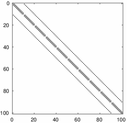
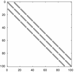
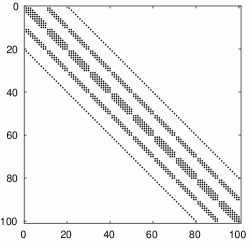
In the GMRF method for fields on a rectangular mesh, we assume that a variable on a gridpoint is conditionally independent on the rest of the gridpoints, given values on neighboring gridpoints. It follows that nonzero entries in the inverse of the covariance matrix can be only between neighbor gridpoints. We start with 4 neighbors (up, down, right, left), and adding neighbors gives rise to a sequence of nested covariance models. If the columns of the mesh are stacked vertically, their inverse covariance matrix will have a band-diagonal structure.

The inverse covariance model fitted by MLE was introduced by Ueno  Tsuchiya (2009) and applied on data from oceanography. The corresponding Fisher information matrix may be found as the negative of the Hessian matrix (Ueno  Tsuchiya, 2009, eq. (C17)).

Figure 1: Block band-diagonal structure of inverse covariance matrix. 10 columns of dimension 10, stacked vertically. 4, 8, 12 neighbors of any gridpoint.

5 COMPUTATIONAL STUDY

In Section 3, we have shown that in the sense of asymptotic variance and second moment (mean-squared) error, the maximum likelihood estimator computed in a smaller space containing the true parameter is more (or equally) precise. For small samples, we illustrate this behavior by means of simulations.

5.1 Simulation of simple GMRF

We first show that in the case of GMRF with four neighbors per gridpoint, adding dependencies (parameters) which are not present brings a loss of precision of the MLE. Using the sample covariance in this case causes a substantial error.

We have generated an ensemble of realizations of a GMRF with dimensions $10\times 10$ (resulting in $n=100$) and inverse covariance structure as in Fig. 1. The values on the diagonals of the covariance matrix have been set to constant, since we assume the correlation with left and right neighbor to be identical, as well as the correlation with upper and lower neighbor (by symmetry of the covariance matrix and isotropy in both directions of the field, but different correlation in each direction). This leads to a model with 3 parameters for 4 neighbors, 5 parameters for 8 neighbors and 7 parameters for 12 neighbors,

The covariance structure of $\Sigma^{-1}$ with 4 neighbors was set as “truth” and random samples were generated from $\mathcal{N}_{n}(\bm{0},\Sigma)$ with sample sizes $N=10,15,20,\ldots,55$. The values on first, second and tenth diagonal have been set as 5, -0.2 and 0.5. For each sample, we computed successively the MLE with 3, 5 and 7 unknown parameters numerically by Newton’s method, as described in Ueno  Tsuchiya (2009).

The difference of each estimator from the true matrix $\Sigma$ was measured in the Frobenius norm, which is the same as the Euclidean norm of a matrix written as one long vector. In order to reduce the sampling error, 50 simulations of the same size were generated and the mean of squared Frobenius norm was computed. The results can be found in Fig. 2.

Figure 2: Error of the MLE in Frobenius norm for sample covariance and models with 4, 8, 12 neighbors, i.e. 5, 9, 13 nonzero diagonals in the inverse covariance matrix.

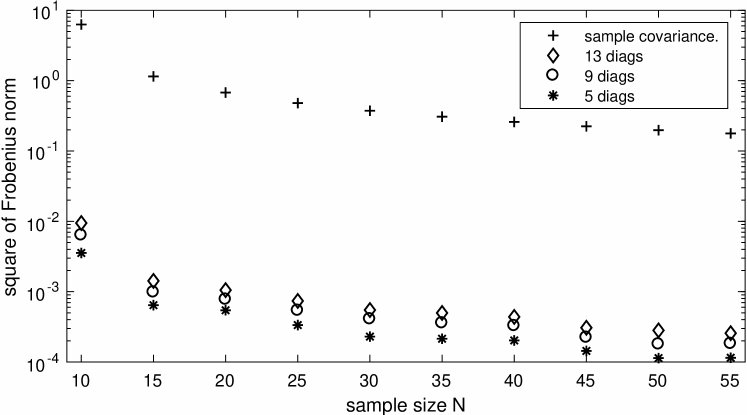
As expected, the MLE with 3 parameters outperforms the estimates with 5 and 7 parameters and the Frobenius norm for sample covariance stays one order worse than all parametric estimates.

5.2 Simulation of fields with diagonal covariance

The simulation for spectral diagonal covariance was carried out in a similar way. First, a diagonal matrix $D$ was prepared, whose diagonal entries decay according to the model $d_{i}=\frac{1}{c}e^{\alpha\lambda_{i}},i=1,\ldots,n$, where $c$ and $\alpha$ are parameters and $\lambda_{i}$ are the eigenvalues of Laplace operator in two dimensions on $10\times 10$ nodes (so again $n=100$). Such models are useful in modeling smooth random fields, e.g., in meteorology. Then, random samples were generated from $\mathcal{N}_{n}(\bm{0},D)$ with sample sizes $N=5,\ldots,20$. For each sample, four covariance matrix estimators were computed:

• sample covariance matrix $\hat{\Sigma}_{N}$, cf. (14)

• diagonal part $\hat{D}^{\left(0\right)}$ of the sample covariance matrix, cf. (15)

• MLE $\hat{D}^{\left(1\right)}$ in the space of diagonal matrices, cf. (18)

• MLE $\hat{D}^{\left(3\right)}=\operatorname{diag}\{(\hat{c}_{1}-\hat{c}_{2}\lambda_{i})^{-1}e^{\hat{\alpha}\lambda_{i}},i=1,\ldots,n\}$ with 3 parameters $c_{1},c_{2}$ and $\alpha$, cf. (24).

• MLE $\hat{D}^{\left(2\right)}=\operatorname{diag}\{\hat{c}^{-1}e^{\hat{\alpha}\lambda_{i}},i=1,\ldots,n\}$ with 2 parameters $c$ and $\alpha$, cf. (28).

Let us briefly discuss the choice of the covariance model $d_{i}=\frac{1}{c}e^{\alpha\lambda_{i}}$. We decided to carry out the simulation with a second-order stationary random field, whose covariance can be diagonalized by the Fourier transform. This transform is formed by the eigenvectors of the Laplace operator. Hence, it is reasonable to model the diagonal terms of this covariance matrix (i.e. the covariance eigenvalues) by some function of eigenvalues of the Laplace operator. This function needs to have a sufficiently fast decay in order to fulfil the necessary condition for the proper covariance (the so-called trace class property, e.g., Kuo (1975)). Exponential decay is used, e.g., in Mirouze  Weaver (2010). Another possible choice of a covariance model is a power model, where the eigenvalues of the covariance are assumed to be a negative power of $-\lambda_{i},i=1,\ldots,n$, e.g., Berner . (2009); Gaspari . (2006); Simpson . (2012).

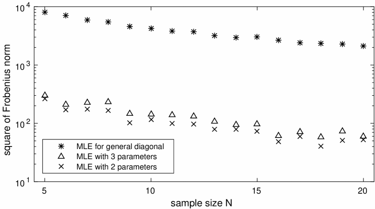
The difference of each estimator from the true matrix $D$ was measured in the Frobenius norm again. To reduce the sampling noise, 50 replications have been done for each sample size and the mean of squared Frobenius norm can be found in Fig. 3.

Figure 3: Comparison of the error matrix $\hat{D}-D$ in the Frobenius norm. The field had dimension $n=10\times 10$. Exponential decay of eigenvalues (i.e. $\tau_{i}=ce^{\alpha\lambda_{i}},i=1,\ldots,n$ ) was used with parameters $c=1/30$ and $\alpha=0.002$. The full line is the order of convergence $\mathrm{const}(N^{-1})$ fitted to the error of the sample covariance.

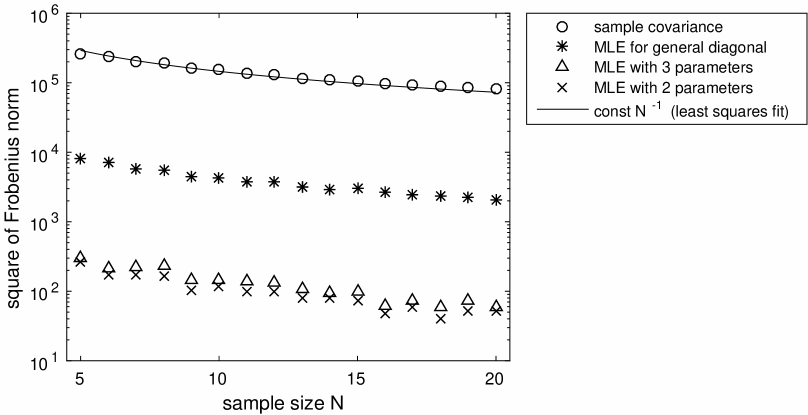
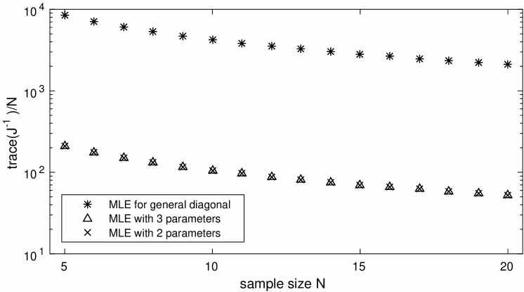
For the diagonal MLE, given by (18), (24), and (28), we can expect from (12) that these estimators should satisfy asymptotically

$$\operatorname{E}\left(\left|\hat{D}_{N}^{\left(k\right)}-D\right|_{F}^{2}\right)\approx\frac{1}{N}\operatorname*{Tr}(J_{D^{\left(k\right)}}^{-1}),\quad k=1,2,3,$$ (30)

even if convergence in distribution does not imply convergence of moments without additional assumptions. This conjecture can be supported by a comparison of Figures 5 and 4, where we observe the same decay. From the nesting, we know that

$$\operatorname*{Tr}(J_{D^{\left(2\right)}}^{-1})\leq\operatorname*{Tr}(J_{D^{\left(3\right)}}^{-1})\leq\operatorname*{Tr}(J_{D^{\left(1\right)}}^{-1})$$ (31)

and we can expect that the Frobenius norm should decrease for more restrictive models, that is,

$$\operatorname{E}\left|\hat{D}_{N}^{\left(2\right)}-D\right|_{F}^{2}\leq\operatorname{E}\left|\hat{D}_{N}^{\left(3\right)}-D\right|_{F}^{2}\leq\operatorname{E}\left|\hat{D}_{N}^{\left(1\right)}-D\right|_{F}^{2},$$ (32)

which is confirmed by the simulations (see Figure 4, resp. 5).

The comparisons (32) of the Frobenius norm of the error in the mean squared complement the pointwise comparison (16) between the sample covariance and its diagonal. Relying on MLE for that comparison is not practical, because the sample size of interest here is $N<n$, and, consequently, $\hat{\Sigma}_{N}$ is singular and cannot be cast as MLE with an accompanying Fisher information matrix, cf. Remark 6. But it is evident that for small sample sizes, estimators computed in the proper subspace perform better. Hence, the hierarchical order seems to hold even when $N<n$.

Figure 4: $\frac{1}{N}\operatorname*{Tr}(J^{-1}_{D})$ for the three parameterizations.

Figure 5: Mean of $|\hat{D}_{N}^{\left(k\right)}-D|_{F}^{2}$ based on 50 replications

6 COMPARISON WITH REGULARIZATION METHODS

In the previous sections, we pointed out the advantages of using low-parametric models for estimating a covariance matrix using a small sample. As mentioned in the Introduction, there is another large class of estimating methods for high-dimensional covariance matrices: shrinkage estimators. The principle of these methods is to move the sample covariance towards a target matrix that possesses some desired properties (e.g., full rank, proper structure). This can be seen as a convex combination of the sample covariance matrix $\hat{\Sigma}_{N}$ and the so called target matrix $T$:

$$\hat{\Sigma}_{S}=\gamma\hat{\Sigma}_{N}+(1-\gamma)T,\hskip 14.22636pt\text{ for }\gamma\in[0,1].$$ (33)

One of the simplest shrinkage estimators has the form of (33) with the target matrix equal to identity, which results in shrinking all sample eigenvalues with the same intensity towards their mean value. Ledoit  Wolf (2004) derived the optimal shrinkage parameter $\gamma$ to minimize the squared Frobenius loss

$$\min_{\gamma}\operatorname{E}||\hat{\Sigma}_{S}-D||_{F}^{2}.$$ (34)

The comparison of this estimator with the maximum likelihood estimator $\hat{D}^{(2)}$ was accomplished by a simulation with identical setting as in Section 5. The results are shown in Fig. 6. For reference, the sample covariance $\hat{\Sigma}_{N}$ and its diagonal $\hat{D}^{(0)}$ are also added.

Another regularization method is described in Won . (2013). They consider a type of covariance estimator, where the regularization effect is achieved by bounding the condition number of the estimate by a regularization parameter $\kappa_{max}$. Since the condition number is defined as a ratio of the largest and smallest eigenvalue, this method corrects for overestimation of the largest eigenvalues and underestimation of the small eigenvalues simultaneously. The resulting estimator is called a condition-number-regularized covariance estimator and it is formulated as the maximum likelihood estimator restricted on the subspace of matrices with condition number bounded by $\kappa_{max}$, i.e.

$$\max_{\Sigma}\ell(\Sigma)\hskip 11.38109pt\text{ subject to }\frac{\lambda_{max}(\Sigma)}{\lambda_{min}(\Sigma)}\leq\kappa_{max},$$ (35)

where $\lambda_{max}(\Sigma)$, resp. $\lambda_{min}(\Sigma)$, is the largest, resp. the smallest, eigenvalue of the covariance matrix $\Sigma$. An optimal $\kappa_{max}$ is selected by maximization of the expected likelihood, which is approximated by using $K$-fold cross-validation. The authors proved that $\kappa_{max}$ selected in this way is a consistent estimator for the true condition number (i.e. the condition number of $D$). Therefore, the idea of this method is to search a MLE in a subspace defined by covariance matrices with condition number smaller or equal to the true condition number. The form of the resulting covariance estimator together with the details of the computational process is provided in Won . (2013). In Fig. 6, we can see the performance of this estimator (denoted as cond-num-regularization) in comparison of other methods.

Figure 6: Comparison of regularization estimators with maximum likelihood estimators. The error matrices $\hat{\Sigma}-D$ are compared in the Frobenius norm. The simulation setting was identical with the Section 5.

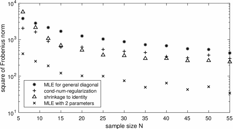
The shrinkage estimator $\hat{\Sigma}_{S}$ and the condition-number-regularized estimator result in non-diagonal matrices, which in our case predetermines them to perform worse than the diagonal estimator $\hat{D}^{(0)}$. However, we have to note that performance of these methods strongly depends on the particular form of the true covariance matrix $D$. In the case when the decrease of the true eigenvalues is less rapid, both methods may provide better results than the diagonal of sample covariance. The performance of $\hat{\Sigma}_{S}$ could be possibly improved by choosing a different target matrix that is closer to reality but such a study is out of the scope of this paper.

It is seen from Fig. 6 that the condition-number-regularized estimator provides more precise estimates than the sample covariance $\hat{\Sigma}_{N}$, as expected. This is in accordance with the preceding theory and empirical findings about the higher precision of estimators from a smaller parametric subspace (the corresponding parametric subspace consists of matrices with the condition number smaller or equal to $\kappa_{max}$). If, however, the theoretical condition number is very large as in our case, the method has a problem in estimating this number and its performance is limited.

Both regularization estimators perform well against sample covariance, but the setting of our simulation is less favourable for them. Neither of them can compete with the maximum likelihood estimator found in the true small subspace of diagonal matrices with proper decay.

7 CONCLUSIONS

Our main aim was to point out the significant advantage resulting from computing the MLE of the covariance matrix in a proper parameter subspace, especially in the high-dimensional setting, when the available sample has small size relative to the dimension of the problem. This subspace can be formed, e.g., by a parametric model for covariance eigenvalues or for a diagonal matrix resulting from a suitable set of transformations.

We provided theoretical results on asymptotic comparison of covariance matrices of each estimator for multivariate normal distribution, where we can lean on the well-developed maximum likelihood theory. The situation for small samples was illustrated by means of a simulation. We consider two-parametric models for the covariance eigenvalues based on the eigenvalues of Laplace operator. In practice, the proper model/subspace can be inferred from historical data.

Using a properly specified model, one can reach a significant improvement in performance, which can have a positive impact on the subsequent tasks like data assimilation and prediction.

BIBLIOGRAPHY

- Bannister (\APACyear2008) \APACinsertmetastarBannister-2008-RFE{APACrefauthors}Bannister, R\BPBIN. \APACrefYearMonthDay2008. \BBOQ\APACrefatitleA review of forecast error covariance statistics in atmospheric variational data assimilation. II: Modelling the forecast error covariance statistics A review of forecast error covariance statistics in atmospheric variational data assimilation. II: Modelling the forecast error covariance statistics.\BBCQ \APACjournalVolNumPagesQuarterly Journal of the Royal Meteorological Society1346371971–1996. {APACrefDOI} \doi10.1002/qj.340 \PrintBackRefs\CurrentBib
- Beezley \BOthers. (\APACyear2011) \APACinsertmetastarBeezley-2011-WEK{APACrefauthors}Beezley, J\BPBID., Mandel, J.\BCBL \BBA Cobb, L. \APACrefYearMonthDay2011. \BBOQ\APACrefatitleWavelet Ensemble Kalman Filters Wavelet ensemble Kalman filters.\BBCQ \BIn \APACrefbtitleProceedings of IEEE IDAACS’2011, Prague, September 2011 Proceedings of IEEE IDAACS’2011, Prague, September 2011 (\BVOL 2, \BPGS 514–518). \APACaddressPublisherIEEE. {APACrefDOI} \doi10.1109/IDAACS.2011.6072819 \PrintBackRefs\CurrentBib
- Berner \BOthers. (\APACyear2009) \APACinsertmetastarBerner-2009-SSK{APACrefauthors}Berner, J., Shutts, G\BPBIJ., Leutbecher, M.\BCBL \BBA Palmer, T\BPBIN. \APACrefYearMonthDay2009. \BBOQ\APACrefatitleA Spectral Stochastic Kinetic Energy Backscatter Scheme and Its Impact on Flow-Dependent Predictability in the ECMWF Ensemble Prediction System A spectral stochastic kinetic energy backscatter scheme and its impact on flow-dependent predictability in the ECMWF ensemble prediction system.\BBCQ \APACjournalVolNumPagesJournal of the Atmospheric Sciences663603–626. {APACrefDOI} \doi10.1175/2008JAS2677.1 \PrintBackRefs\CurrentBib
- Buehner \BBA Charron (\APACyear2007) \APACinsertmetastarBuehner-2007-SSL{APACrefauthors}Buehner, M.\BCBT \BBA Charron, M. \APACrefYearMonthDay2007. \BBOQ\APACrefatitleSpectral and spatial localization of background-error correlations for data assimilation Spectral and spatial localization of background-error correlations for data assimilation.\BBCQ \APACjournalVolNumPagesQuarterly Journal of the Royal Meteorological Society133624615–630. {APACrefDOI} \doi10.1002/qj.50 \PrintBackRefs\CurrentBib
- Carlen (\APACyear2010) \APACinsertmetastarCarlen-2010-TIQ{APACrefauthors}Carlen, E. \APACrefYearMonthDay2010. \BBOQ\APACrefatitleTrace inequalities and quantum entropy: an introductory course Trace inequalities and quantum entropy: an introductory course.\BBCQ \BIn \APACrefbtitleEntropy and the quantum Entropy and the quantum (\BVOL 529, \BPGS 73–140). \APACaddressPublisherAmer. Math. Soc., Providence, RI. {APACrefDOI} \doi10.1090/conm/529/10428 \PrintBackRefs\CurrentBib
- Furrer \BBA Bengtsson (\APACyear2007) \APACinsertmetastarFurrer-2007-EHP{APACrefauthors}Furrer, R.\BCBT \BBA Bengtsson, T. \APACrefYearMonthDay2007. \BBOQ\APACrefatitleEstimation of high-dimensional prior and posterior covariance matrices in Kalman filter variants Estimation of high-dimensional prior and posterior covariance matrices in Kalman filter variants.\BBCQ \APACjournalVolNumPagesJ. Multivariate Anal.982227–255. {APACrefDOI} \doi10.1016/j.jmva.2006.08.003 \PrintBackRefs\CurrentBib
- Gaspari \BOthers. (\APACyear2006) \APACinsertmetastarGaspari-2006-CAC{APACrefauthors}Gaspari, G., Cohn, S\BPBIE., Guo, J.\BCBL \BBA Pawson, S. \APACrefYearMonthDay2006. \BBOQ\APACrefatitleConstruction and application of covariance functions with variable length-fields Construction and application of covariance functions with variable length-fields.\BBCQ \APACjournalVolNumPagesQuarterly Journal of the Royal Meteorological Society1326191815–1838. {APACrefDOI} \doi10.1256/qj.05.08 \PrintBackRefs\CurrentBib
- Hamill \BBA Snyder (\APACyear2000) \APACinsertmetastarHamill-2000-HEK{APACrefauthors}Hamill, T\BPBIM.\BCBT \BBA Snyder, C. \APACrefYearMonthDay2000. \BBOQ\APACrefatitleA Hybrid Ensemble Kalman Filter–3D Variational Analysis Scheme A hybrid ensemble Kalman filter–3D variational analysis scheme.\BBCQ \APACjournalVolNumPagesMonthly Weather Review12882905–2919. {APACrefDOI} \doi10.1175/1520-0493(2000)128¡2905:AHEKFV¿2.0.CO;2 \PrintBackRefs\CurrentBib
- Kasanický \BOthers. (\APACyear2015) \APACinsertmetastarKasanicky-2015-SDE{APACrefauthors}Kasanický, I., Mandel, J.\BCBL \BBA Vejmelka, M. \APACrefYearMonthDay2015. \BBOQ\APACrefatitleSpectral diagonal ensemble Kalman filters Spectral diagonal ensemble Kalman filters.\BBCQ \APACjournalVolNumPagesNonlinear Processes in Geophysics224485 – 497. {APACrefDOI} \doi10.5194/npg-22-485-2015 \PrintBackRefs\CurrentBib
- Kuo (\APACyear1975) \APACinsertmetastarKuo-1975-GMB{APACrefauthors}Kuo, H\BPBIH. \APACrefYear1975. \APACrefbtitleGaussian measures in Banach spaces Gaussian measures in Banach spaces. \APACaddressPublisherBerlinSpringer-Verlag. {APACrefDOI} \doi10.1007/BFb0082008 \PrintBackRefs\CurrentBib
- Lauritzen (\APACyear1996) \APACinsertmetastarlauritzen1996graphical{APACrefauthors}Lauritzen, S\BPBIL. \APACrefYear1996. \APACrefbtitleGraphical models Graphical models (\BVOL 17). \APACaddressPublisherClarendon Press. \PrintBackRefs\CurrentBib
- Ledoit \BBA Wolf (\APACyear2004) \APACinsertmetastarLedoit-2004-WEL{APACrefauthors}Ledoit, O.\BCBT \BBA Wolf, M. \APACrefYearMonthDay2004. \BBOQ\APACrefatitleA well-conditioned estimator for large-dimensional covariance matrices A well-conditioned estimator for large-dimensional covariance matrices.\BBCQ \APACjournalVolNumPagesJ. Multivariate Anal.882365–411. {APACrefDOI} \doi10.1016/S0047-259X(03)00096-4 \PrintBackRefs\CurrentBib
- Lehmann \BBA Casella (\APACyear1998) \APACinsertmetastarLehmann-1998-TPE{APACrefauthors}Lehmann, E\BPBIL.\BCBT \BBA Casella, G. \APACrefYear1998. \APACrefbtitleTheory of point estimation Theory of point estimation (\PrintOrdinalSecond \BEd). \APACaddressPublisherSpringer-Verlag, New York. {APACrefDOI} \doi10.1007/b98854 \PrintBackRefs\CurrentBib
- Magnus \BBA Neudecker (\APACyear2007) \APACinsertmetastarMagnus-2007-MDC{APACrefauthors}Magnus, J\BPBIR.\BCBT \BBA Neudecker, H. \APACrefYear2007. \APACrefbtitleMatrix Differential Calculus with Applications in Statistics and Econometrics Matrix differential calculus with applications in statistics and econometrics (\PrintOrdinalThird \BEd). \APACaddressPublisherJohn Wiley. \PrintBackRefs\CurrentBib
- Mandel \BOthers. (\APACyear2010) \APACinsertmetastarMandel-2010-FFT{APACrefauthors}Mandel, J., Beezley, J\BPBID.\BCBL \BBA Kondratenko, V\BPBIY. \APACrefYearMonthDay2010. \BBOQ\APACrefatitleFast Fourier Transform Ensemble Kalman Filter with Application to a Coupled Atmosphere-Wildland Fire Model Fast Fourier transform ensemble Kalman filter with application to a coupled atmosphere-wildland fire model.\BBCQ \BIn A\BPBIM. Gil-Lafuente \BBA J\BPBIM. Merigo (\BEDS), \APACrefbtitleComputational Intelligence in Business and Economics, Proceedings of MS’10 Computational Intelligence in Business and Economics, Proceedings of MS’10 (\BPGS 777–784). \APACaddressPublisherWorld Scientific. {APACrefDOI} \doi10.1142/9789814324441_0089 \PrintBackRefs\CurrentBib
- Michel \BBA Auligné (\APACyear2010) \APACinsertmetastarMichel-2010-IBE{APACrefauthors}Michel, Y.\BCBT \BBA Auligné, T. \APACrefYearMonthDay2010. \BBOQ\APACrefatitleInhomogeneous Background Error Modeling and Estimation over Antarctica Inhomogeneous Background Error Modeling and Estimation over Antarctica.\BBCQ \APACjournalVolNumPagesMonthly Weather Review13862229–2252. {APACrefDOI} \doi10.1175/2009mwr3139.1 \PrintBackRefs\CurrentBib
- Mirouze \BBA Weaver (\APACyear2010) \APACinsertmetastarMirouze-2010-RCF{APACrefauthors}Mirouze, I.\BCBT \BBA Weaver, A\BPBIT. \APACrefYearMonthDay2010. \BBOQ\APACrefatitleRepresentation of correlation functions in variational assimilation using an implicit diffusion operator Representation of correlation functions in variational assimilation using an implicit diffusion operator.\BBCQ \APACjournalVolNumPagesQuarterly Journal of the Royal Meteorological Society1361421–1443. {APACrefDOI} \doi10.1002/qj.643 \PrintBackRefs\CurrentBib
- Muirhead (\APACyear2005) \APACinsertmetastarMuirhead-2005-AMS{APACrefauthors}Muirhead, R. \APACrefYear2005. \APACrefbtitleAspects of Multivariate Statistical Theory Aspects of multivariate statistical theory. \APACaddressPublisherWiley. {APACrefDOI} \doi10.1002/9780470316559 \PrintBackRefs\CurrentBib
- Pannekoucke \BOthers. (\APACyear2007) \APACinsertmetastarPannekoucke-2007-FPW{APACrefauthors}Pannekoucke, O., Berre, L.\BCBL \BBA Desroziers, G. \APACrefYearMonthDay2007. \BBOQ\APACrefatitleFiltering Properties of Wavelets For Local Background-Error Correlations Filtering properties of wavelets for local background-error correlations.\BBCQ \APACjournalVolNumPagesQuarterly Journal of the Royal Meteorological Society133623, Part B363–379. {APACrefDOI} \doi10.1002/qj.33 \PrintBackRefs\CurrentBib
- Parrish \BBA Derber (\APACyear1992) \APACinsertmetastarParrish-1992-NMC{APACrefauthors}Parrish, D\BPBIF.\BCBT \BBA Derber, J\BPBIC. \APACrefYearMonthDay1992. \BBOQ\APACrefatitleThe National Meteorological Center’s Spectral Statistical-Interpolation Analysis System The National Meteorological Center’s spectral statistical-interpolation analysis system.\BBCQ \APACjournalVolNumPagesMonthly Weather Review12081747–1763. {APACrefDOI} \doi10.1175/1520-0493(1992)120¡1747:TNMCSS¿2.0.CO;2 \PrintBackRefs\CurrentBib
- Rao (\APACyear1973) \APACinsertmetastarRao-1973-LSI{APACrefauthors}Rao, C\BPBIR. \APACrefYear1973. \APACrefbtitleLinear statistical inference and its applications Linear statistical inference and its applications (\PrintOrdinalSecond \BEd). \APACaddressPublisherJohn Wiley & Sons, New York-London-Sydney. \APACrefnoteWiley Series in Probability and Mathematical Statistics {APACrefDOI} \doi10.1002/9780470316436 \PrintBackRefs\CurrentBib
- Rue \BBA Held (\APACyear2005) \APACinsertmetastarrue2005gaussian{APACrefauthors}Rue, H.\BCBT \BBA Held, L. \APACrefYear2005. \APACrefbtitleGaussian Markov random fields: theory and applications Gaussian Markov random fields: theory and applications. \APACaddressPublisherCRC Press. \PrintBackRefs\CurrentBib
- Schäfer \BBA Strimmer (\APACyear2005) \APACinsertmetastarSchafer-2005-SAL{APACrefauthors}Schäfer, J.\BCBT \BBA Strimmer, K. \APACrefYearMonthDay2005. \BBOQ\APACrefatitleA shrinkage approach to large-scale covariance matrix estimation and implications for functional genomics A shrinkage approach to large-scale covariance matrix estimation and implications for functional genomics.\BBCQ \APACjournalVolNumPagesStatistical Applications in Genetics and Molecular Biology4Article number 32. {APACrefDOI} \doi10.2202/1544-6115.1175 \PrintBackRefs\CurrentBib
- Simpson \BOthers. (\APACyear2012) \APACinsertmetastarSimpson-2012-TCM{APACrefauthors}Simpson, D., Lindgren, F.\BCBL \BBA Rue, H. \APACrefYearMonthDay2012. \BBOQ\APACrefatitleThink continuous: Markovian Gaussian models in spatial statistics Think continuous: Markovian Gaussian models in spatial statistics.\BBCQ \APACjournalVolNumPagesSpatial Statistics116–29. {APACrefDOI} \doi10.1016/j.spasta.2012.02.003 \PrintBackRefs\CurrentBib
- Ueno \BBA Tsuchiya (\APACyear2009) \APACinsertmetastarUeno-2009-CRI{APACrefauthors}Ueno, G.\BCBT \BBA Tsuchiya, T. \APACrefYearMonthDay2009. \BBOQ\APACrefatitleCovariance regularization in inverse space Covariance regularization in inverse space.\BBCQ \APACjournalVolNumPagesQuarterly Journal of the Royal Meteorological Society1356421133–1156. {APACrefDOI} \doi10.1002/qj.445 \PrintBackRefs\CurrentBib
- Vershynin (\APACyear2012) \APACinsertmetastarVershynin-2012-HCS{APACrefauthors}Vershynin, R. \APACrefYearMonthDay2012. \BBOQ\APACrefatitleHow close is the sample covariance matrix to the actual covariance matrix? How close is the sample covariance matrix to the actual covariance matrix?\BBCQ \APACjournalVolNumPagesJ. Theoret. Probab.253655–686. {APACrefDOI} \doi10.1007/s10959-010-0338-z \PrintBackRefs\CurrentBib
- Wang \BOthers. (\APACyear2008) \APACinsertmetastarWang-2008-HE3{APACrefauthors}Wang, X., Barker, D\BPBIM., Snyder, C.\BCBL \BBA Hamill, T\BPBIM. \APACrefYearMonthDay2008. \BBOQ\APACrefatitleA hybrid ETKF–3DVAR data assimilation scheme for the WRF model. Part I: Observing system simulation experiment A hybrid ETKF–3DVAR data assimilation scheme for the WRF model. Part I: Observing system simulation experiment.\BBCQ \APACjournalVolNumPagesMonthly Weather Review136125116–5131. {APACrefDOI} \doi10.1175/2008MWR2444.1 \PrintBackRefs\CurrentBib
- Won \BOthers. (\APACyear2013) \APACinsertmetastarWon-2013-CCE{APACrefauthors}Won, J\BHBIH., Lim, J., Kim, S\BHBIJ.\BCBL \BBA Rajaratnam, B. \APACrefYearMonthDay2013. \BBOQ\APACrefatitleCondition-number-regularized covariance estimation Condition-number-regularized covariance estimation.\BBCQ \APACjournalVolNumPagesJ. R. Stat. Soc. Ser. B. Stat. Methodol.753427–450. {APACrefDOI} \doi10.1111/j.1467-9868.2012.01049.x \PrintBackRefs\CurrentBib