Mode volume, energy transfer, and spaser threshold in plasmonic systems with gain

Abstract

We present a unified approach to describe spasing in plasmonic systems modeled by quantum emitters interacting with resonant plasmon mode. We show that spaser threshold implies detailed energy transfer balance between the gain and plasmon mode and derive explicit spaser condition valid for arbitrary plasmonic systems. By defining carefully the plasmon mode volume relative to the gain region, we show that the spaser condition represents, in fact, the standard laser threshold condition extended to plasmonic systems with dispersive dielectric function. For extended gain region, the saturated mode volume depends solely on the system parameters that determine the lower bound of threshold population inversion.

I Introduction

The prediction of plasmonic laser (spaser) bergman-prl03 ; stockman-natphot08 ; stockman-jo10 and its experimental realization in various systems noginov-nature09 ; zhang-nature09 ; zheludev-oe09 ; zhang-natmat10 ; ning-prb12 ; gwo-science12 ; odom-natnano13 ; shalaev-nl13 ; gwo-nl14 ; zhang-natnano14 ; odom-natnano15 have been among the highlights in the rapidly developing field of plasmonics during the past decade stockman-review . First observed in gold nanoparticles (NP) coated by dye-doped silics shells noginov-nature09 , spasing action was reported in hybrid plasmonic waveguides zhang-nature09 , semiconductor quantum dots on metal film zheludev-oe09 ; gwo-nl14 , plasmonic nanocavities and nanocavity arrays zhang-natmat10 ; ning-prb12 ; gwo-science12 ; odom-natnano13 ; zhang-natnano14 ; odom-natnano15 , and metallic NP and nanorods noginov-nature09 ; shalaev-nl13 , and more recently, carbon-based structures apalkov-light14 ; premaratne-acsnano14 . Small spaser size well below the diffraction limit gives rise to wealth of applications stockman-aop17 .

The spaser feedback mechanism is based on the near-field coupling between resonant plasmon mode and gain medium, modeled here by an ensemble of pumped two-level quantum emitters (QE) with excitation frequency tuned to the plasmon frequency. The spaser threshold condition has been suggested as bergman-prl03 ; stockman-natphot08 ; stockman-jo10

$$\frac{4\pi\mu^{2}\tau_{2}}{3\hbar}\frac{N_{21}}{\cal V}\,Q\simeq 1,$$ (1)

where $\mu$ and $\tau_{2}$ are the QE dipole matrix element and polarization relaxation time, respectively, $N_{21}=N_{2}-N_{1}$ is the ensemble population inversion ($N_{2}$ and $N_{1}$ are, respectively, the number of excited and ground-state QEs), $Q$ is the mode quality factor, and ${\cal V}$ is the mode volume. Equation (1) is similar to the standard laser condition haken that determines the threshold value of $N_{21}$, but with the cavity mode quality factor and volume replaced by their plasmon counterparts in metal-dielectric system characterized by dispersive dielectric function $\varepsilon(\omega,\bm{r})$. While the plasmon quality factor $Q$ is well-defined in terms of the metal dielectric function $\varepsilon(\omega)=\varepsilon^{\prime}(\omega)+i\varepsilon^{\prime\prime}(\omega)$, there is an active debate on mode volume definition in plasmonic systems maier-oe06 ; polman-nl10 ; koenderink-ol10 ; hughes-ol12 ; russel-prb12 ; lalanne-prl13 ; hughes-acsphot14 ; bonod-prb15 ; muljarov-prb16 ; shegai-oe16 ; derex-jo16 . Since QEs are usually distributed outside the plasmonic structure, the standard expression for cavity mode volume, $\int dV\varepsilon(\bm{r})|\textbf{E}(\bm{r})|^{2}/\text{max}[\varepsilon(\bm{r})|\textbf{E}(\bm{r})|^{2}]$, where $\textbf{E}(\bm{r})$ is the mode electric field, is ill-defined for open systems koenderink-ol10 ; hughes-ol12 ; hughes-acsphot14 . Furthermore, defining the plasmon mode volume in terms of field intensity at a specific point maier-oe06 ; lalanne-prl13 seems impractical due to very large local field variations near the metal surface caused by particulars of system geometry, for example, sharp edges or surface imperfections: strong field fluctuations would grossly underestimate the mode volume that determines spasing threshold for gain distributed in an extended region. At the same time, while spasing was theoretically studied for several specific systems wegener-oe08 ; stockman-jo10 ; klar-bjn13 ; li-prb13 ; lisyansky-oe13 ; bordo-pra13 , the general spaser condition was derived, in terms of system parameters such as permittivities and optical constants, only for two-component systems stockman-prl11 ; stockman-review without apparent relation to the mode volume in Eq. (1). Note that the actual spasing systems can be comprised of many components, so that the extension of the laser condition (1) to plasmonics implies some procedure, valid for any nanoplasmonic system, to determine the plasmon mode volume.

On the other hand, the steady state spaser action implies detailed balance of energy transfer (ET) processes between the QEs and the plasmon mode (see Fig. 1). Whereas the energy flow between individual QEs and plasmon can go in either direction depending on the QE quantum state, the net gain-plasmon ET rate is determined by population inversion $N_{21}$ and, importantly, distribution of plasmon states in the gain region. Since individual QE-plasmon ET rates are proportional to the plasmon local density of states (LDOS), which can vary in a wide range depending on QEs’ positions and system geometry shahbazyan-prl16 , the net ET rate is obtained by averaging the plasmon LDOS over the gain region. Therefore, the plasmon mode volume should relate, in terms of average system characteristics, the laser condition (1) to the microscopic gain-plasmon ET picture. The goal of this paper is to establish such a relation.

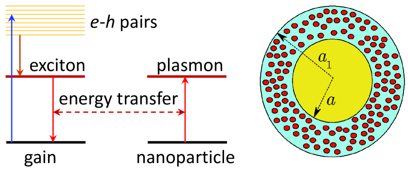
Figure 1: Spaser energy transfer diagram (left) and schematics for metal nanoparticle with dye-doped dielectric shell (right).

First, we derive the general spaser condition for any multicomponent nanoplasmonic system in terms of individual ET rates between QEs, constituting the gain, and resonant plasmon mode, providing the feedback. Second, we introduce the plasmon mode volume $\mathcal{V}$ associated with a region of volume $V_{0}$ by relating $\mathcal{V}$ to the plasmon LDOS, averaged over that region, and establish that the spaser condition does have the general form (1). We then demonstrate, analytically and numerically, that a sufficiently extended region outside the plasmonic structure can saturate the plasmon mode volume, in which case $\mathcal{V}$ is independent of the plasmon field distribution and determined solely by the system parameters,

$$\frac{{\cal V}}{V_{0}}=Q\,\varepsilon_{d}\,\frac{\varepsilon^{\prime\prime}(\omega_{pl})}{|\varepsilon^{\prime}(\omega_{pl})|},$$ (2)

where $\varepsilon_{d}$ is the gain region dielectric constant and $\omega_{pl}$ is the plasmon frequency. With saturated mode volume (2), the laser condition (1) matches the spaser condition for two-component systems stockman-prl11 ; stockman-review and, in fact, defines the lower bound of threshold $N_{21}$. Finally, we demonstrate that, in realistic systems, the threshold $N_{21}$ can significantly exceed its minimal value.

II Spasing and gain-plasmon energy transfer balance

We consider $N_{0}$ QEs described by pumped two-level systems, located at positions $\textbf{r}_{j}$ near a plasmonic structure, with excitation energy $\hbar\omega_{21}=E_{2}-E_{1}$, where $E_{1}$ and $E_{2}$ are, respectively, the lower and upper level energies. Within the density matrix approach, each QE is described by polarization $\rho_{21}^{(j)}$ and occupation $n_{21}^{(j)}\equiv\rho_{22}^{(j)}-\rho_{11}^{(j)}$, so that $N_{21}=N_{2}-N_{1}=\sum_{j}n_{21}^{(j)}$ is the ensemble population inversion. In the rotating wave approximation, the steady-state dynamics of QEs coupled to alternating electric field $\bm{\mathcal{\cal E}}(\bm{r})e^{-i\omega t}$ is described by the Maxwell-Bloch equations

$$\left(\omega-\omega_{21}+i/\tau_{2}\right)\rho_{21}^{(j)}=\frac{\mu}{\hbar}\,n_{21}^{(j)}\,\bm{n}_{j}\!\cdot\!\bm{\mathcal{\cal E}}(\bm{r}_{j}),$$ (3)

$$n_{21}^{(j)}-\bar{n}_{21}=-\frac{4\mu\tau_{1}}{\hbar}\,\text{Im}\!\left[\rho_{21}^{(j)*}\,\bm{n}_{j}\!\cdot\!\bm{\mathcal{\cal E}}(\bm{r}_{j})\right],$$

where $\tau_{2}$ and $\tau_{1}$ are the time constants characterizing polarization and population relaxation, $\mu$ and $\bm{n}_{j}$ are, respectively, the QE dipole matrix element and orientation, and $\bar{n}_{21}$ is the average population inversion per QE due to the pump. The local field $\bm{\mathcal{\cal E}}(\bm{r}_{j})$ at the QE position is generated by all QEs’ dipole moments $\bm{p}_{j}=\mu\bm{n}_{j}\rho_{21}^{(j)}$ and, within semiclassical approach, has the form novotny-book

$$\bm{\mathcal{\cal E}}(\bm{r}_{j})=\frac{4\pi\omega^{2}}{c^{2}}\sum_{k}\bar{\textbf{G}}(\omega;\bm{r}_{j},\bm{r}_{k})\!\cdot\!\bm{p}_{k},$$ (4)

where $\bar{\textbf{G}}(\omega;\bm{r},\bm{r}^{\prime})$ is the electromagnetic Green dyadic in the presence of metal nanostructure and $c$ is the speed of light. For nanoplasmonic systems, it is convenient to adopt rescaled Green dyadic that has direct near-field limit, $\bar{\textbf{D}}(\omega;\bm{r},\bm{r}^{\prime})=-(4\pi\omega^{2}/c^{2})\bar{\textbf{G}}(\omega;\bm{r},\bm{r}^{\prime})$. Upon eliminating the electric field, the system (3) takes the form

$$\Omega_{21}\bm{p}_{j}+\frac{\mu^{2}}{\hbar}\,n_{21}^{(j)}\bm{n}_{j}\sum_{k}\bm{n}_{j}\!\cdot\!\bar{\textbf{D}}(\omega;\bm{r}_{j},\bm{r}_{k})\!\cdot\!\bm{p}_{k}=0,$$

$$\frac{\delta n_{21}^{j}}{\tau_{1}}-\frac{4}{\hbar}\,\text{Im}\sum_{k}\left[\bm{p}_{j}^{*}\!\cdot\!\bar{\textbf{D}}(\omega;\bm{r}_{j},\bm{r}_{k})\!\cdot\!\bm{p}_{k}\right]=0,$$ (5)

where we use shorthand notations $\Omega_{21}=\omega-\omega_{21}+i/\tau_{2}$ and $\delta n_{21}^{j}=n_{21}^{(j)}-\bar{n}_{21}$. The first equation in system (II), being homogeneous in $\bm{p}_{j}$, leads to the spaser threshold condition. Since the Green dyadic includes contributions from all electromagnetic modes, the spaser threshold in general case can only be determined numerically. However, for QEs coupled to a resonant plasmon mode, that is, for $\omega_{21}$ close to the mode frequency $\omega_{pl}$, the contribution from off-resonance modes is relatively small pustovit-prb16 ; petrosyan-17 and, as we show below, the spaser condition can be obtained explicitly for any nanoplasmonic system.

II.1 Gain coupling to a resonant plasmon mode

For QE frequencies $\omega_{21}$ close to the plasmon frequency $\omega_{pl}$, we can adopt the single mode approximation for the Green dyadic shahbazyan-prl16

$$\bar{\textbf{D}}(\omega;\bm{r},\bm{r}^{\prime})=\frac{\omega_{pl}}{4U}\frac{\textbf{E}(\bm{r})\otimes\textbf{E}^{*}(\bm{r}^{\prime})}{\omega-\omega_{pl}+i/\tau_{pl}},$$ (6)

where $\textbf{E}(\bm{r})$ is the slow envelope of plasmon field satisfying the Gauss law $\bm{\nabla}\cdot\left[\varepsilon^{\prime}(\omega_{pl},\bm{r})\textbf{E}(\bm{r})\right]=0$ and $1/\tau_{pl}$ is the plasmon decay rate. In nanoplasmonic systems, the decay rate is dominated by the Ohmic losses and has the form

$$\dfrac{1}{\tau_{pl}}=\dfrac{W}{2U},$$ (7)

where

$$U=\frac{1}{16\pi}\!\int\!dV\left|\textbf{E}(\bm{r})\right|^{2}\partial\left[\omega_{pl}\varepsilon^{\prime}(\omega_{pl},\bm{r})\right]/\partial\omega_{pl}$$ (8)

is the mode stored energy, and

$$W=\frac{\omega_{pl}}{8\pi}\!\int\!dV\left|\textbf{E}(\bm{r})\right|^{2}\varepsilon^{\prime\prime}(\omega_{pl},\bm{r})$$ (9)

is the mode dissipated power landau . The volume integration in $U$ and $W$ takes place, in fact, only over the metallic regions with dispersive dielectric function. For systems with a single metallic region, one obtains the standard plasmon decay rate:

$$\frac{1}{\tau_{pl}}=\frac{\varepsilon^{\prime\prime}(\omega_{pl})}{\partial\varepsilon^{\prime}(\omega_{pl})/\partial\omega_{pl}}.$$ (10)

The Green dyadic (6) is valid for a well-defined plasmon mode ($\omega_{pl}\tau_{pl}\gg 1$) in any nanoplasmonic system, and its consistency is ensured by the optical theorem shahbazyan-prl16 .

With the plasmon Green dyadic (6), the system (II) takes the form

$$\Omega_{21}\bm{p}_{j}+\frac{\mu^{2}}{\hbar}\frac{\omega_{pl}n_{21}^{(j)}}{4U\Omega_{pl}}\,\bm{n}_{j}[\bm{n}_{j}\!\cdot\!\textbf{E}(\bm{r}_{j})]\sum_{k}\textbf{E}^{*}(\bm{r}_{k})\!\cdot\!\bm{p}_{k}=0,$$

$$\frac{\delta n_{21}^{j}}{\tau_{1}}-\text{Im}\biggl{[}\frac{\omega_{pl}}{\hbar U\Omega_{pl}}\,[\bm{p}_{j}^{*}\!\cdot\!\textbf{E}(\bm{r}_{j})]\sum_{k}\textbf{E}^{*}(\bm{r}_{k})\!\cdot\!\bm{p}_{k}\biggr{]}=0,$$ (11)

where $\Omega_{pl}=\omega-\omega_{pl}+i/\tau_{pl}$. Multiplying the first equation by $\textbf{E}^{*}(\bm{r}_{j})$ and summing up over $j$, we obtain the spaser condition

$$\Omega_{21}\Omega_{pl}+\frac{\mu^{2}}{\hbar}\frac{\omega_{pl}}{4U}\sum_{j}n_{21}^{(j)}\left|\bm{n}_{j}\!\cdot\!\textbf{E}(\bm{r}_{j})\right|^{2}=0.$$ (12)

The second term in Eq. (12) describes coherent coupling between the QE ensemble and plasmon mode. Below we show that spasing implies detailed ET balance between the gain and plasmon mode.

II.2 Energy transfer and spaser condition

Let us now introduce, in the standard manner, the individual QE-plasmon ET rate as shahbazyan-prl16

$$\frac{1}{\tau}=-\frac{\mu^{2}}{\hbar}\text{Im}\!\left[\bm{n}\!\cdot\!\bar{\textbf{D}}(\omega_{pl};\bm{r},\bm{r})\!\cdot\!\bm{n}\right]=\!\frac{4\pi\mu^{2}}{\hbar}\frac{|\bm{n}\!\cdot\!\textbf{E}(\bm{r})|^{2}}{\int\!dV\varepsilon^{\prime\prime}|\textbf{E}|^{2}},$$ (13)

where we used Eqs. (6) and (7), and implied $\varepsilon\equiv\varepsilon(\omega_{pl},\bm{r})$ under the integral. The condition (12) can be recast as

$$\left(\omega-\omega_{21}+\frac{i}{\tau_{2}}\right)\left(\omega-\omega_{pl}+\frac{i}{\tau_{pl}}\right)+\frac{1}{\tau_{g}\tau_{pl}}=0,$$ (14)

where we introduced net gain-plasmon ET rate,

$$\frac{1}{\tau_{g}}=\sum_{j}\frac{n_{21}^{(j)}}{\tau_{j}}=\frac{4\pi\mu^{2}}{\hbar}\sum_{j}n_{21}^{(j)}\,\frac{|\bm{n}_{j}\!\cdot\!\textbf{E}(\bm{r}_{j})|^{2}}{\int\!dV\varepsilon^{\prime\prime}|\textbf{E}|^{2}},$$ (15)

which represents the sum of individual QE-plasmon ET rates $1/\tau_{j}$, given by Eq. (13), weighed by QE occupation numbers. Since $n_{21}^{(j)}$ is positive or negative for QE in the excited or ground state, respectively, the direction of energy flow between the QE and the plasmon mode depends on the QE quantum state. Note that the main contribution to $1/\tau_{g}$ comes from the regions with large plasmon LDOS, that is, high QE-plasmon ET rates (13). The imaginary part of Eq. (14) yields the spaser frequency bergman-prl03

$$\omega_{s}=\frac{\omega_{pl}\tau_{pl}+\omega_{21}\tau_{2}}{\tau_{pl}+\tau_{2}},$$ (16)

while its real part, with the above $\omega_{s}$, leads to

$$\frac{1}{\tau_{g}\tau_{pl}}=\frac{1}{\tau_{2}\tau_{pl}}+\frac{\left(\omega_{pl}-\omega_{21}\right)^{2}\tau_{2}\tau_{pl}}{(\tau_{pl}+\tau_{2})^{2}}.$$ (17)

In the case when the QE and plasmon spectral bands overlap well, that is., $|\omega_{pl}-\omega_{21}|\tau_{pl}\ll 1$ or $|\omega_{pl}-\omega_{21}|\tau_{2}\ll 1$ depending on relative magnitude of the respective bandwidths $1/\tau_{2}$ and $1/\tau_{pl}$, the last term in Eq. (17) can be disregarded, and we arrive at the spaser condition in the form $1/\tau_{g}=1/\tau_{2}$, or

$$\sum_{j}\frac{n_{21}^{(j)}}{\tau_{j}}=\frac{1}{\tau_{2}}.$$ (18)

Equation (18) implies that spaser threshold is reached when energy transfer balance between gain and plasmon mode is established.

II.3 System geometry and QE-plasmon ET rate

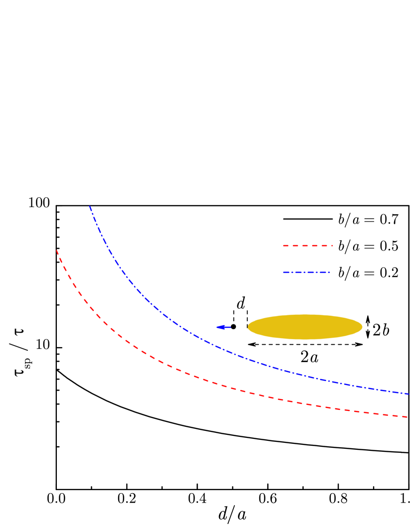
Figure 2: QE-plasmon ET rate (13) for a QE near a spheroidal particle with aspect ratio $b/a$ normalized by that for spherical particle with radius $a$.

Individual ET rates in the spaser condition (18) can vary in a wide range depending on the QE position and system geometry. In Fig. 2, we show the ET rate (13) for a QE located at distance $d$ from a tip of gold nanorod, modeled here by prolate spheroid with semiaxes $a$ and $b$ (see Appendix). In all numerical calculations, we use the experimental dielectric function for gold christy . To highlight the role of system geometry, the ET rate $1/\tau$ for nanorod is normalized by the ET rate $1/\tau_{sp}$ for sphere of radius $a$. The latter ET rate has the form

$$\frac{1}{\tau_{sp}}=\frac{12\mu^{2}}{\hbar\varepsilon^{\prime\prime}(\omega_{sp})}\frac{a^{3}}{(a+d)^{6}},$$ (19)

and experiences a sharp decrease for $d>a$. With changing nanoparticle shape, three degenerate dipole modes of a sphere split into longitudinal and two transverse modes. The latter move up in energy to get damped by interband transitions in gold with their onset just above the plasmon energy in spherical particles, while the longitudinal mode moves down in energy away from the transitions onset, thereby gaining in the oscillator strength mulvaney-prl02 . This sharpening of plasmon resonance together with condensation of plasmon states near the tips (lightning rod effect) results in up to 100-fold rate increase with reducing $b/a$ ratio, as shown in Fig. 2, indicating that spasing is dominated by QEs located in the large plasmon LDOS regions. Large variations of $1/\tau$ magnitude imply that the plasmon mode volume, which characterizes spatial extent of the gain region with sufficiently strong QE-plasmon coupling, is determined by the average plasmon LDOS in that region, as we show in the next section.

III Plasmon mode volume and spaser threshold

III.1 General spaser condition

The form (18) of spaser condition reveals the microscopic origin of spaser action as the result of cooperative ET between gain and resonant plasmon mode, with each QE contribution depending on its position and quantum state. Below we assume that QEs are distributed within some region of volume $V_{0}$ and that population inversion distribution follows, on average, that of QEs. After averaging over QEs’ dipole orientations, the gain-plasmon ET rate (15) takes the form

$$\frac{1}{\tau_{g}}=\frac{4\pi\mu^{2}}{3\hbar}\frac{\int\!dV_{0}n_{21}(\bm{r})|\textbf{E}(\bm{r})|^{2}}{\int\!dV\varepsilon^{\prime\prime}(\omega_{pl},\bm{r})|\textbf{E}(\bm{r})|^{2}},$$ (20)

where $n_{21}(\bm{r})$ is population inversion density, yielding the spaser threshold condition

$$\frac{4\pi\mu^{2}\tau_{2}}{3\hbar}\frac{\int\!dV_{0}n_{21}(\bm{r})|\textbf{E}(\bm{r})|^{2}}{\int\!dV\varepsilon^{\prime\prime}(\omega_{pl},\bm{r})|\textbf{E}(\bm{r})|^{2}}=1,$$ (21)

which is valid for any multicomponent system supporting a well-defined surface plasmon. In the case of uniform gain distribution, $n_{21}=N_{21}/V_{0}$, and a single metallic component with volume $V_{m}$ [e.g., a metal particle with dye-doped dielectric shell (see Fig. 1)], the threshold condition (21) takes the form

$$\frac{4\pi\mu^{2}\tau_{2}}{3\hbar}\,\frac{n_{21}}{\varepsilon^{\prime\prime}(\omega_{pl})}\,\frac{\int\!dV_{0}|\textbf{E}|^{2}}{\int\!dV_{m}|\textbf{E}|^{2}}=1.$$ (22)

The threshold value of $n_{21}$ is determined by ratio of plasmon field integral intensities in the gain and metal regions. Evidently, the spaser threshold does depend on the gain region size and shape, which prompts us to revisit the mode volume definition for plasmonic systems in order to ensure its consistency with the general laser condition (1).

III.2 Plasmon LDOS and associated mode volume

Here, we show that the mode volume in plasmonic systems can be accurately defined in terms of plasmon LDOS. The LDOS of a single plasmon mode is related to the plasmon Green dyadic (6) as $\rho(\omega,\bm{r})=-(2\pi^{2}\omega_{pl})^{-1}\,\text{Im}\,\text{Tr}\,\bar{\textbf{D}}(\omega;\bm{r},\bm{r})$, and has the Lorentzian form shahbazyan-prl16 ,

$$\rho(\omega,\bm{r})=\frac{\tau_{pl}}{8\pi^{2}U}\frac{\left|\textbf{E}(\bm{r})\right|^{2}}{(\omega-\omega_{pl})^{2}\tau_{pl}^{2}+1},$$ (23)

where $U$ is given by Eq. (8). The plasmon LDOS (23) characterizes the distribution of plasmon states in the unit volume and frequency interval. Consequently, its frequency integral, $\rho(\bm{r})=\!\int\!d\omega\rho(\omega,\bm{r})$, represents the plasmon mode density that describes the plasmon states’ spatial distribution:

$$\rho(\bm{r})=\frac{\left|\textbf{E}(\bm{r})\right|^{2}}{8\pi U}=\frac{2\left|\textbf{E}(\bm{r})\right|^{2}}{\int\!dV[\partial(\omega_{pl}\varepsilon^{\prime})/\partial\omega_{pl}]|\textbf{E}|^{2}}.$$ (24)

Introducing the mode quality factor $Q=\omega_{pl}U/W$, the mode density can be written as

$$\rho(\bm{r})=\frac{1}{Q}\frac{\left|\textbf{E}(\bm{r})\right|^{2}}{\int\!dV\varepsilon^{\prime\prime}|\textbf{E}|^{2}}.$$ (25)

Note that, in terms of $\rho(\bm{r})$, the gain-plasmon ET rate (20) takes the form

$$\frac{1}{\tau_{g}}=\frac{4\pi\mu^{2}}{3\hbar}\,Q\int\!dV_{0}n_{21}(\bm{r})\rho(\bm{r}),$$ (26)

implying that the largest contribution to $1/\tau_{g}$ comes from QEs located in the regions with high plasmon density.

We now relate the plasmon mode volume ${\cal V}$ associated with region $V_{0}$ to the average mode density in that region:

$$\frac{1}{\mathcal{V}}=\frac{1}{V_{0}}\!\int\!dV_{0}\rho(\bm{r})=\frac{1}{V_{0}}\frac{2\int\!dV_{0}\left|\textbf{E}\right|^{2}}{\int\!dV[\partial(\omega_{pl}\varepsilon^{\prime})/\partial\omega_{pl}]|\textbf{E}|^{2}},$$ (27)

or, equivalently,

$$\frac{\mathcal{V}}{V_{0}}=Q\,\frac{\int\!dV\varepsilon^{\prime\prime}|\textbf{E}|^{2}}{\int\!dV_{0}|\textbf{E}|^{2}}.$$ (28)

The expressions (27) or (28) are valid for nanoplasmonic systems of any size and shape and with any number of metallic and dielectric components.

It is straightforward to check that, for uniform gain distribution with $n_{21}=N_{21}/V_{0}$, the spaser threshold condition (21) coincides with the laser condition (1) with associated mode volume $\mathcal{V}$ given by Eq. (28). Equivalently, for uniform gain distribution, the gain-plasmon ET rate (26) takes the form

$$\frac{1}{\tau_{g}}=\frac{4\pi\mu^{2}}{3\hbar}\,\frac{N_{21}}{\mathcal{V}}\,Q,$$ (29)

and the laser condition (1) follows from the ET balance condition $1/\tau_{g}=1/\tau_{2}$.

For systems with single metal component, the plasmon mode volume takes the form [compare to Eq. (22)]

$$\frac{\mathcal{V}}{V_{0}}=\frac{\omega_{pl}}{2}\frac{\partial\varepsilon^{\prime}(\omega_{pl})}{\partial\omega_{pl}}\frac{\int\!dV_{m}|\textbf{E}|^{2}}{\int\!dV_{0}|\textbf{E}|^{2}}=Q\,\varepsilon^{\prime\prime}(\omega_{pl})\,\frac{\int\!dV_{m}|\textbf{E}|^{2}}{\int\!dV_{0}|\textbf{E}|^{2}},$$ (30)

where the plasmon quality factor has the form

$$Q=\omega_{pl}\,\frac{\partial\varepsilon^{\prime}(\omega_{pl})/\partial\omega_{pl}}{2\varepsilon^{\prime\prime}(\omega_{pl})}=\frac{\omega_{pl}\tau_{pl}}{2}.$$ (31)

Note that, for a well-defined plasmon with $Q\gg 1$, the plasmon mode volume is independent of Ohmic losses in metal.

III.3 Mode volume saturation and lower bound of spaser threshold

Since the QE-plasmon ET rate rapidly falls outside the plasmonic structure (see Fig. 2), spasing is dominated by QEs located sufficiently close to the metal surface. In the case when a metal nanostructure of volume $V_{m}$ is surrounded by an extended gain region $V_{0}$, so that the plasmon LDOS spillover beyond $V_{0}$ is negligible, the plasmon mode volume is saturated by the gain, leading to constant value of ${\cal V}/V_{0}$ that is independent of the plasmon field distribution. To demonstrate this point, we note that, in the quasistatic approximation, the integrals in Eq. (30) reduce to surface terms,

$$\int\!dV_{0}|\textbf{E}|^{2}=\int\!dS\,\Phi^{*}\nabla_{n}\Phi+\!\int\!dS_{1}\Phi^{*}\nabla_{n}\Phi,$$

$$\int\!dV_{m}|\textbf{E}|^{2}=\int\!dS\,\Phi^{*}\nabla_{n}\Phi,$$ (32)

where $S$ is the common interface separating the metal and dielectric regions, $S_{1}$ is the outer boundary of the dielectric region, $\Phi$ is the potential related to the plasmon field as $\textbf{E}=-\bm{\nabla}\Phi$, and $\nabla_{n}\Phi$ is its normal derivative relative to the interface. The potentials in the first and second equations of system (III.3) are taken, respectively, at the dielectric and metal sides of the interface $S$. Since the plasmon fields rapidly fall away from the metal, the contribution from the outer interface $S_{1}$ can be neglected for extended dielectric regions (see below). Then, using the standard boundary conditions at the common interface $S$, we obtain from Eqs. (30) and (III.3) the saturated mode volume:

$$\frac{\mathcal{V}}{V_{0}}=\frac{\omega_{pl}\varepsilon_{d}}{2|\varepsilon^{\prime}(\omega_{pl})|}\frac{\partial\varepsilon^{\prime}(\omega_{pl})}{\partial\omega_{pl}}=Q\,\varepsilon_{d}\,\frac{\varepsilon^{\prime\prime}(\omega_{pl})}{|\varepsilon^{\prime}(\omega_{pl})|}.$$ (33)

Remarkably, the saturated mode volume depends on system geometry only via the plasmon frequency $\omega_{pl}$ in the metal dielectric function. Combining Eqs. (33) and (1), we arrive at the spaser condition for saturated case,

$$\frac{4\pi\mu^{2}\tau_{2}}{3\hbar\varepsilon_{d}}\frac{|\varepsilon^{\prime}(\omega_{pl})|}{\varepsilon^{\prime\prime}(\omega_{pl})}\,n_{21}=1,$$ (34)

which matches the spaser condition obtained previously for two-component systems, that is, with gain region extended to infinity stockman-review ; stockman-prl11 . We stress that the condition (34) provides the lower bound for threshold value of $n_{21}$, while in real systems, where plasmon field distribution can extend beyond the gain region, the threshold can be significantly higher, as we illustrate below.

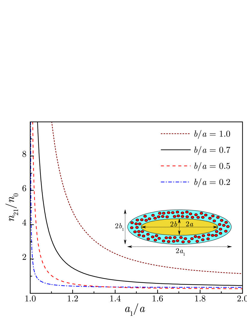
Figure 3: Calculated threshold $n_{21}$ for gold nanorods with dye-doped silica shell is shown with increasing gain region size. Rapid plasmon mode volume saturation for small $b/a$ is due to condensation of plasmon states near the nanorod tips.

In Fig. (3), we show the change of threshold $n_{21}$ with expanding gain region in nanorod-based spaser modeled by composite spheroidal particle with gold core and QE-doped silica shell. Calculations were performed using Eq. (22) for confocal spheroids (see Appendix for details), and QE frequency $\omega_{21}$ was tuned to resonance with longitudinal dipole mode frequency $\omega_{pl}$. Note that the gain optical constants enter the spaser condition (22) through a single parameter

$$n_{0}=\frac{3\hbar}{4\pi\mu^{2}\tau_{2}},$$ (35)

which represents characteristic gain concentration and sets the overall scale of threshold $n_{21}$ for a specific gain medium. The ratio $n_{21}/n_{0}$, plotted in Fig. 3, depends only on plasmonic system parameters and, with expanding gain region, decreases prior reaching plateau corresponding to the saturated mode volume regime described by Eq. (34). Note that, in nanorods, the rapid mode volume saturation seen in Fig. 3, as compared to spherical particles, is caused by condensation of plasmon states near the tips (lightning rod effect), leading to the much larger plasmon LDOS and, correspondingly, the QE-plasmon ET rate (see Fig. 2).

IV Conclusions

In summary, we have developed a unified approach to spasing in a system of pumped quantum emitters interacting with a plasmonic structure of arbitrary shape in terms of energy transfer processes within the system. The threshold value of population inversion is determined from the condition of detailed energy transfer balance between quantum emitters, constituting the gain, and resonant plasmon mode, providing the feedback. We have shown that, in plasmonic systems, the mode volume should be defined relative to a finite region, rather than to a point of maximal field intensity, by averaging the plasmon local density of states over that region. We demonstrated that, in terms of plasmon mode volume, the spaser condition has the standard form of the laser threshold condition, thus, extending the latter to plasmonic systems with dispersive dielectric function. We have also shown that, for extended gain region, the saturated plasmon mode volume is determined solely by the system permittivities, which define the lower bound of threshold population inversion.

Appendix A Calculation of QE-plasmon ET rate for spheroidal nanoparticle

The ET rate between a plasmon mode in metal nanoparticle with frequency $\omega_{pl}$ and a QE located at the point $\bm{r}$ distanced by $d$ from the metal surface and polarized along the normal $\bm{n}$ to the surface is given by

$$\frac{1}{\tau}=\frac{4\pi\mu^{2}}{\hbar}\frac{|\bm{n}\!\cdot\!\textbf{E}(\bm{r})|^{2}}{\int\!dV\varepsilon^{\prime\prime}|\textbf{E}|^{2}}=\frac{4\pi\mu^{2}}{\hbar\varepsilon^{\prime\prime}(\omega_{pl})}\frac{|{\nabla}_{n}\Phi(\bm{r})|^{2}}{\int\!dS\Phi^{*}{\nabla}_{n}\Phi},$$ (36)

where $\nabla_{n}=\bm{n}\!\cdot\!\bm{\nabla}$ stands for the normal derivative, and real part of the denominator is implied.

Consider a QE at distance $d$ from the tip of a spheroidal particle with semiaxis $a$ along the symmetry axis and semiaxis $b$ in the symmetry plane ($a>b$). The potentials have the form $\Phi\propto R_{lm}(\xi)Y_{lm}(\eta,\zeta)$, where $\xi$ is the radial (normal) coordinate and the pair $(\eta,\zeta)$ parametrizes the surface ($Y_{lm}$ are spherical harmonics). The surface area element is $dS=h_{\eta}h_{\zeta}d\eta d\zeta$, and normal derivative is $\nabla_{n}=h_{\xi}^{-1}(\partial/\partial\xi)$, where $h_{i}$ are the scale factors ($i=\xi,\eta,\zeta$) given by

$$h_{\xi}=f\sqrt{\frac{\xi^{2}-\eta^{2}}{\xi^{2}-1}},~{}~{}h_{\eta}=f\sqrt{\frac{\xi^{2}-\eta^{2}}{1-\eta^{2}}},$$

$$h_{\zeta}=f\sqrt{(\xi^{2}-1)(1-\eta^{2})},$$ (37)

$f=\sqrt{a^{2}-b^{2}}$ is half distance between the foci, and spheroid surface corresponds to $\xi_{1}=a/f$.

For QE located at point $z=f\xi$ on the $z$-axis ($\eta=1$) outside the spheroid, the radial potentials for dipole longitudinal plasmon mode $(lm)=(10)$ have the form $R(\xi)=P_{1}(\xi)$ for $\xi<\xi_{1}$ and $R(\xi)=Q_{1}(\xi)P_{1}(\xi_{1})/Q_{1}(\xi_{1})$ for $\xi>\xi_{1}$, where $P_{l}$ and $Q_{l}$ are the Legendre functions of first and second kind, given by

$$P_{1}(\xi)=\xi,~{}~{}Q_{1}(\xi)=\frac{\xi}{2}\ln\left(\frac{\xi+1}{\xi-1}\right)-1,$$

$$Q^{\prime}_{1}(\xi)=\frac{1}{2}\ln\left(\frac{\xi+1}{\xi-1}\right)-\frac{\xi}{\xi^{2}-1}.$$ (38)

Using $h_{\xi}=f$ along the $z$-axis, the ET rate equals

$$\frac{1}{\tau}=\frac{3\mu^{2}}{\hbar\varepsilon^{\prime\prime}(\omega_{pl})}\frac{R^{\prime 2}(\xi)}{f^{3}\xi_{1}(\xi_{1}^{2}-1)}=\frac{3\mu^{2}}{\hbar ab^{2}\varepsilon^{\prime\prime}(\omega_{pl})}\left[\frac{Q^{\prime}_{1}(\xi)\xi_{1}}{Q_{1}(\xi_{1})}\right]^{2},$$ (39)

with $\xi=(a+d)/f$, where the plasmon frequency $\omega_{pl}$ determined by the boundary condition $\varepsilon^{\prime}(\omega_{pl})=\varepsilon_{d}Q^{\prime}_{1}(\xi_{1})$. In the limit of spherical particle of radius $a$, that is, $f\rightarrow 0$ and $\xi\rightarrow\infty$ as $b\rightarrow a$, we have $Q(\xi)\approx 1/3\xi^{2}$, yielding

$$\frac{1}{\tau_{sp}}=\frac{12\mu^{2}}{\hbar\varepsilon^{\prime\prime}(\omega_{sp})}\frac{a^{3}}{(a+d)^{6}},$$ (40)

where $\omega_{sp}$ is surface plasmon resonance frequency for a sphere determined by $\varepsilon^{\prime}(\omega_{sp})+2\varepsilon_{d}=0$. The normalized ET rate $\tau_{sp}/\tau$ has the form

$$\frac{\tau_{sp}}{\tau}=\frac{a^{2}}{4b^{2}}\left(1+\frac{d}{a}\right)^{6}\frac{\varepsilon^{\prime\prime}(\omega_{sp})}{\varepsilon^{\prime\prime}(\omega_{pl})}\left[\frac{Q^{\prime}_{1}(\xi)\xi_{1}}{Q_{1}(\xi_{1})}\right]^{2},$$ (41)

with $\xi=\xi_{1}+d/f$.

Appendix B Calculation of population inversion density in spheroidal core-shell nanoparticle

We consider a core-shell nanoparticle with dielectric functions $\varepsilon_{c}$, $\varepsilon_{s}$, and $\varepsilon_{d}$ in the core, shell, and outside dielectric, respectively, with inner and outer interface $S_{1}$ and $S_{2}$. The integrals over core ans shell regions in the condition (22) reduce to surface terms

$$\int\!dV_{c}|\textbf{E}|^{2}=\!\int\!dS_{1}\Phi^{*}E_{n}^{c},$$

$$\int\!dV_{s}|\textbf{E}|^{2}=\!\int\!dS_{2}\Phi^{*}E_{n}^{s}-\!\int\!dS_{1}\Phi^{*}E_{n}^{s},$$ (42)

where $E_{n}^{j}(S_{i})=-\nabla_{jn}\Phi(S_{i})$ is the field outward normal component at the $i$th interface in the $j$th medium side. Note that $E_{n}^{s}(S_{1})=(\varepsilon_{c}/\varepsilon_{s})E_{n}^{c}(S_{1})$ and $E_{n}^{s}(S_{2})=(\varepsilon_{d}/\varepsilon_{s})E_{n}^{d}(S_{2})$. The ratio of integrated field intensities in the shell and core regions takes the form

$$L=\frac{\!\int\!dV_{s}|\textbf{E}|^{2}}{\!\int\!dV_{c}|\textbf{E}|^{2}}=\frac{\varepsilon_{d}}{\varepsilon_{s}}\frac{\int\!dS_{2}\Phi^{*}E_{n}^{d}}{\int\!dS_{1}\Phi^{*}E_{n}^{c}}-\frac{\varepsilon_{c}}{\varepsilon_{s}},$$ (43)

where the potentials $\Phi$ are continuous at the interfaces. For nanostructures whose shape permits separation of variables, the potential can be written as $\Phi(\bm{r})=R(\xi)\Sigma(\eta,\zeta)$, where $\xi$ is the radial (normal) coordinate and the pair $(\eta,\zeta)$ parametrizes the surface. With surface area element $dS=h_{\eta}h_{\zeta}d\eta d\zeta$ and normal derivative $\nabla_{n}=h_{\xi}^{-1}(\partial/\partial\xi)$, where $h_{i}$ are the scale factors ($i=\xi,\eta,\zeta$), the fraction of integrals takes the form

$$I=\frac{\int\!dS_{2}\Phi^{*}E_{n}^{d}}{\int\!dS_{1}\Phi^{*}E_{n}^{c}}= \frac{R_{d}(\xi_{2})R_{d}^{\prime}(\xi_{2})}{R_{c}(\xi_{1})R_{c}^{\prime}(\xi_{1})}$$

$$\times \frac{\int\!\int\!d\eta_{2}d\zeta_{2}(h_{\eta_{2}}h_{\zeta_{2}}/h_{\xi_{2}})|\Sigma|^{2}}{\int\!\int\!d\eta_{1}d\zeta_{1}(h_{\eta_{1}}h_{\zeta_{1}}/h_{\xi_{1}})|\Sigma|^{2}}.$$ (44)

Below we outline evaluation of $L$ for core-shell NP described by two confocal prolate spheroids with semi-axises $a$ and $b$. The two shell surfaces corresponds to $\xi_{1}=a/f$ and $\xi_{2}=sa/f$, where $f=\sqrt{a^{2}-b^{2}}$ is half distance between the foci, and $s>1$ characterizes the shell thickness. Evaluation of angular integrals yields

$$I=\frac{R_{d}(\xi_{2})R_{d}^{\prime}(\xi_{2})}{R_{c}(\xi_{1})R_{c}^{\prime}(\xi_{1})}\,\frac{\xi_{2}^{2}-1}{\xi_{1}^{2}-1}.$$ (45)

For longitudinal dipole mode ($l=1$, $m=0$), we have $R_{c}=P_{1}(\xi)$ for $\xi<\xi_{1}$, $R_{s}=AP_{1}(\xi)+BQ_{1}(\xi)$ for $\xi_{2}<\xi<\xi_{2}$, and $R_{d}=CQ_{1}(\xi)$ for $\xi>\xi_{2}$, yielding

$$L=C^{2}\,\frac{\varepsilon_{d}}{\varepsilon_{s}}\,\frac{Q_{1}(\xi_{2})Q^{\prime}_{1}(\xi_{2})}{P_{1}(\xi_{1})P^{\prime}_{1}(\xi_{1})}\,\frac{\xi_{2}^{2}-1}{\xi_{1}^{2}-1}-\frac{\varepsilon_{c}}{\varepsilon_{s}},$$ (46)

where $C$ and $\varepsilon_{c}(\omega_{pl})$ are determined from the continuity of $R_{i}$ and $\varepsilon_{i}R^{\prime}_{i}$ across the interfaces.

References

- (1) D. Bergman and M. I. Stockman, Phys. Rev. Lett., 90, 027402, (2003).
- (2) M. I. Stockman, Nature Photonics, 2, 327, (2008).
- (3) M. I. Stockman, J. Opt. 12, 024004, (2010).
- (4) M. A. Noginov, G. Zhu, A. M. Belgrave, R. Bakker, V. M. Shalaev, E. E. Narimanov, S. Stout, E. Herz, T. Suteewong and U. Wiesner, Nature, 460, 1110, (2009).
- (5) R. F. Oulton, V. J. Sorger, T. Zentgraf, R.-M. Ma, C. Gladden, L. Dai, G. Bartal, and X. Zhang, Nature 461, 629, (2009).
- (6) E. Plum, V. A. Fedotov, P. Kuo, D. P. Tsai, and N. I. Zheludev, Opt. Expr. 17, 8548, (2009).
- (7) R. Ma, R. Oulton, V. Sorger, G. Bartal, and X. Zhang, Nature Mater., 10, 110, (2010).
- (8) K. Ding, Z. C. Liu, L. J. Yin, M. T. Hill, M. J. H. Marell, P. J. van Veldhoven, R. Nöetzel, and C. Z. Ning, Phys. Rev. B 85, 041301(R) (2012).
- (9) Y.-J. Lu, J. Kim, H.-Y. Chen, C.i Wu, N. Dabidian, C. E. Sanders, C.-Y. Wang, M.-Y. Lu, B.-H. Li, X. Qiu, W.-H. Chang, L.-J. Chen, G. Shvets, C.-K. Shih, and S. Gwo, Science 337, 450 (2012).
- (10) W. Zhou, M. Dridi, J. Y. Suh, C. H. Kim, D. T. Co, M. R. Wasielewski, G. C. Schatz, and T. W. Odom, Nat. Nano. 8, 506 (2013).
- (11) X. Meng, A. V. Kildishev, K. Fujita, K. Tanaka, and V. M. Shalaev, Nano Lett. 13, 4106, (2013).
- (12) Y. Lu, C.-Y. Wang, J. Kim, H.-Y. Chen, M.-Y. Lu, Y.-C. Chen, W.-H. Chang, L.-J. Chen, M. I. Stockman, C.-K. Shih, S. Gwo, Nano Lett. 14, 4381 (2014).
- (13) R.-M. Ma, S. Ota, Y. Li, S. Yang, and X. Zhang, Nat. Nano. 9, 600 (2014).
- (14) A. Yang, T. B. Hoang, M. Dridi, C. Deeb, M. H. Mikkelsen, G. C. Schatz, and T. W. Odom, Nat. Comm. 6, 6939 (2015).
- (15) M. I. Stockman, in Plasmonics: Theory and Applications, edited by T. V. Shahbazyan and M. I. Stockman (Springer, New York, 2013).
- (16) V. Apalkov and M. I Stockman, Light: Science & Applications 3, e191 (2014).
- (17) C. Rupasinghe, I. D. Rukhlenko, and M. Premaratne, ACS Nano, 8 2431 (2014).
- (18) M. Premaratne and M. I. Stockman, Adv. Opt. Phot. 9, 79 (2017).
- (19) H. Haken, Laser Theory (Springer, New York, 1983).
- (20) M. Wegener, J. L. Garcia-Pomar, C. M. Soukoulis, N. Meinzer, M. Ruther, and S. Linden, Opt. Express 16, 19785 (2008).
- (21) N. Arnold, B. Ding, C. Hrelescu, and T. A. Klar, Beilstein J. Nanotechnol. 4, 974 (2013).
- (22) X.-L. Zhong and Z.-Y. Li, Phys. Rev. B 88, 085101 (2013).
- (23) D. G. Baranov, E.S. Andrianov, A. P. Vinogradov, and A. A. Lisyansky, Opt. Express 21, 10779 (2013).
- (24) V. G. Bordo Phys. Rev. A 88, 013803 (2013).
- (25) S. Maier, Opt. Express 14, 1957 (2006).
- (26) M. Kuttge, F. J. Garcia de Abajo, and A. Polman, Nano Lett. 10, 1537 (2010).
- (27) A. F. Koenderink, Opt. Lett. 35 4208 (2010).
- (28) P. T. Kristensen, C. Van Vlack, and S. Hughes, Opt. Lett. 37, 1649 (2012).
- (29) K. J. Russell, K. Y. M. Yeung, and E. Hu, Phys. Rev. B 85, 245445 (2012).
- (30) C. Sauvan, J. P. Hugonin, I. S. Maksymov, and P. Lalanne, Phys. Rev. Lett. 110, 237401 (2013).
- (31) P. T. Kristensen and S. Hughes, ACS Photon. 1, 2 (2014).
- (32) X. Zambrana-Puyalto, and N. Bonod, Phys. Rev. B 91, 195422 (2015).
- (33) E. A. Muljarov, W. Langbein, Phys. Rev. B 94, 235438 (2016)
- (34) Z.-J. Yang, T. J. Antosiewicz, and T. Shegai, Opt. Express 24, 20373 (2016).
- (35) G. Colas des Francs, J. Barthes, A. Bouhelier, J.C. Weeber, A. Dereux, J. Opt. 18, 094005 (2016).
- (36) M. I. Stockman, Phys. Rev. Lett., 106, 156802, (2011).
- (37) T. V. Shahbazyan, Phys. Rev. Lett. 117, 207401 (2016).
- (38) L. Novotny and B. Hecht, Principles of Nano-Optics (CUP, New York, 2012).
- (39) V. N. Pustovit, A. M. Urbas, A. V. Chipouline, and T. V. Shahbazyan, Phys. Rev. B 93, 165432 (2016).
- (40) L. S. Petrosyan and T. V. Shahbazyan, arXiv:1702.04761.
- (41) L. D. Landau and E. M. Lifshitz, Electrodynamics of Continuous Media (Elsevier, Amsterdam, 2004).
- (42) P. B. Johnson and R.W. Christy, Phys. Rev. B, 6, 4370, (1973).
- (43) C. Sönnichsen, T. Franzl, T. Wilk, G. von Plessen, J. Feldmann, O. V. Wilson, and P. Mulvaney, Phys. Rev. Lett. 88, 077402 (2002).