Ensemble Estimation of Generalized Mutual Information with Applications to Genomics

Abstract

Mutual information is a measure of the dependence between random variables that has been used successfully in myriad applications in many fields. Generalized mutual information measures that go beyond classical Shannon mutual information have also received much interest in these applications. We derive the mean squared error convergence rates of kernel density-based plug-in estimators of general mutual information measures between two multidimensional random variables $\mathbf{X}$ and $\mathbf{Y}$ for two cases: 1) $\mathbf{X}$ and $\mathbf{Y}$ are continuous; 2) $\mathbf{X}$ and $\mathbf{Y}$ may have a mixture of discrete and continuous components. Using the derived rates, we propose an ensemble estimator of these information measures called GENIE by taking a weighted sum of the plug-in estimators with varied bandwidths. The resulting ensemble estimators achieve the $1/N$ parametric mean squared error convergence rate when the conditional densities of the continuous variables are sufficiently smooth. To the best of our knowledge, this is the first nonparametric mutual information estimator known to achieve the parametric convergence rate for the mixture case, which frequently arises in applications (e.g. variable selection in classification). The estimator is simple to implement and it uses the solution to an offline convex optimization problem and simple plug-in estimators. A central limit theorem is also derived for the ensemble estimators and minimax rates are derived for the continuous case. We demonstrate the ensemble estimator for the mixed case on simulated data and apply the proposed estimator to analyze gene relationships in single cell data.

I Introduction

Mutual information (MI) is a measure of the amount of shared information between a pair of random variables $\mathbf{X}$ and $\mathbf{Y}$. MI estimation is related to the problem of estimating functionals of probability distributions, which has received deserved attention in recent years [2, 3, 4, 5, 6, 7, 8, 9, 10, 11, 12, 13, 14, 15, 16, 17]. Many statistical problems rely in some form upon accurate estimation of functionals of probability distributions including estimating the decay rates of error probabilities [18], estimating bounds on the Bayes error rate [19, 20, 21, 22], and hypothesis testing [23, 24, 25]. MI estimation, in particular, also has many applications in information theory and machine learning including independent subspace analysis [26], structure learning [27], fMRI data processing [28], forest density estimation [29], clustering [30], neuron classification [31], blind source separation [32], intrinsically motivated reinforcement learning [33, 34], as well as other data science applications such as sociology [35], computational biology [36, 37, 38], and improving neural network models [39]. A particularly common application is feature selection or extraction where features are chosen to maximize the MI between the chosen features (represented by $\mathbf{X}$) and the outcome variables (represented by $\mathbf{Y}$) [40, 41, 42, 43, 44].

In many of these applications, the variables $\mathbf{X}$ and $\mathbf{Y}$ may have any mixture of discrete and continuous components. In feature selection, for example, the predictor labels may have discrete components (e.g. classification labels) while the input variables may have a mixture of discrete and continuous features. To the best of our knowledge, there are currently no nonparametric MI estimators that are known to achieve the parametric mean squared error (MSE) convergence rate $1/N$ ($N$ is the number of samples) in this setting where $\mathbf{X}$ and/or $\mathbf{Y}$ contain a mixture of discrete and continuous components. Instead, most existing estimators of MI focus on the cases where both $\mathbf{X}$ and $\mathbf{Y}$ are either purely discrete or purely continuous. Also, while many nonparametric estimators of MI exist, most have not been generalized beyond Shannon or Rényi information. Furthermore, minimax convergence rates are currently unknown for the continuous and the mixture cases.

In this paper, we provide a framework for nonparametric estimation of a large class of MI measures where we only have available a finite population of i.i.d. samples. This framework can be applied to accurately estimate general MI measures when either $\mathbf{X}$ and $\mathbf{Y}$ are purely continuous or the mixed case when $\mathbf{X}$ and $\mathbf{Y}$ may contain a mixture of discrete and continuous components. We derive an MI estimator for these cases that achieves the parametric MSE rate when the conditional densities of the continuous variables are sufficiently smooth, thus achieving the minimax rate (which we also derive) in this setting. We call this estimator the Generalized ENsemble Information Estimator (GENIE).

Our estimation method applies to other MI measures in addition to Shannon information, which have been the focus of much recent interest. An information measure based on a quadratic divergence was defined in [40]. A density-resampled version of MI was introduced in [37] to better measure gene relationships in single-cell data when sampling may not be uniform. A MI measure based on the Pearson divergence was considered in [45]. Minimal spanning tree [46] and generalized nearest-neighbor graph [26] approaches have been developed for estimating Rényi information [47, 48, 49], which has been used in many applications (e.g. [50, 51, 32, 52, 53]).

I-A Related Work

Many estimators for MI have been previously developed. Nearly all of these estimators ignore the mixed case and focus on the case where both $\mathbf{X}$ and $\mathbf{Y}$ are either purely continuous or purely discrete. A popular $k$-nearest neighbor (nn)-based estimator was proposed in [54] which is a modification of the entropy estimator derived in [55]. However, these estimators have only been shown to achieve the parametric convergence rate when the dimension of each of the random variables is less than 3 [56]. Furthermore, these estimators focus only on estimating the Shannon MI between purely continuous random variables. Similarly, the estimators in [26, 57] do not achieve the parametric rate and focus on the purely continuous case. An adaptation of the Shannon MI estimator in [54] was recently proposed to handle the discrete-continuous mixture case [2]. While this estimator has been proven to be consistent, its convergence rate is currently unknown. Central limit theorems have also been derived for several entropy estimators [17, 58, 59], which can then be applied to Shannon MI. However, it is not clear if these results can be extended to more general MI functionals.

A neural network-based estimator of Shannon MI was proposed in [39]. While this estimator is computationally efficient, its statistical properties are largely unknown as the authors only prove convergence in probability rates. It is also unclear how to extend this estimator to other MI measures such as the Rényi information. A jackknife approach to estimating Shannon MI was also recently proposed [3]. This approach provides an automatic selection of the kernel bandwidth for a plug-in kernel density estimator (KDE) and does not require boundary correction, which is generally a major difficulty in estimating functionals of probability distributions. However, the MSE convergence rate of this estimator is also unknown.

Much work has focused on the problem of estimating the entropy of purely discrete random variables [60, 4, 5, 6]. Shannon MI can then be estimated by estimating the joint and marginal entropies of $\mathbf{X}$ and $\mathbf{Y}$. However, it is not clear if discrete methods can be extended successfully to the mixed-case. Quantizing the continuous components of the data is one potential approach that has been shown to be consistent for some quantization schemes in the purely continuous case [61] but it is currently unknown if similar approaches can be applied in the mixed-case. Also, extending these estimators to general MI measures like Rényi information is not straightforward.

Recent work has focused on nonparametric divergence estimation for continuous random variables. One approach [7, 8, 9, 10] uses an optimal KDE to achieve the parametric convergence rate when the densities are at least $d$ [9, 10] or $d/2$ [7, 8] times differentiable where $d$ is the dimension of the data. These methods, like ours, assume that the densities are bounded away from zero as this simplifies the analysis. However, this induces a boundary on the densities’ support set. For accurate estimation, the optimal KDE approaches require knowledge of the density support boundary and are difficult to construct near the boundary. Numerical integration may also be required for estimating some divergence functionals under this approach, which can be computationally expensive. In contrast, our approach to MI estimation does not require numerical integration and can be performed without knowledge of the support boundary.

Some methods for estimating distributional functionals have relaxed the boundedness assumption on the densities [62, 63, 17]. These approaches typically assume that the tails of the densities decay at a sufficiently fast rate (e.g. sub-exponential or sub-Gaussian). In [63, 62], the authors only consider densities with up to 2 derivatives as it is difficult to exploit higher smoothness when the densities are not lower-bounded.

More closely related work [11, 13, 12, 17, 14, 64, 15, 16] uses an ensemble approach to estimate entropy or divergence functionals for continuous random variables. These works construct an ensemble of simple plug-in estimators by varying the neighborhood size of density estimators. They then take a weighted average of the estimators where the weights are chosen to decrease the bias with only a small increase in the variance. The parametric rate of convergence is achieved when the densities are either $d$ [11, 13, 12, 15] or $d/2$ [14, 64, 16] times differentiable. These approaches are simple to implement as they only require simple plug-in estimates and the solution of an offline convex optimization problem. The ensemble approach also automatically corrects for bias at the boundary of the densities’ support set.

Finally, [65] showed that $k$-nn or KDE based approaches underestimate the MI when the MI is large. As MI increases, the dependencies between random variables increase which results in less smooth densities. Thus this isn’t an issue when the densities are smooth [7, 8, 9, 10, 11, 13, 12, 14].

For the mixture setting, we focus on the important special case where the components of each observation are assumed to decompose into discrete and continuous dimensions. This enables the density to be factored: $f_{X}(x)=f_{X_{D}}\left(x_{D}\right)f_{X_{C}|X_{D}}\left(x_{C}|x_{D}\right)$ where $x_{C}$ and $x_{D}$ are the continuous and discrete components of $x$. We note that this excludes the more general case considered by [2] where one or more components can have discrete and continuous values simultaneously. However, our setting is a common occurrence in many machine learning and statistical problems. For example, a search within the UCI Machine Learning Repository [66] yields many datasets with such structure. Many statistical models have also focused on similar settings [67, 68, 69, 70]. Thus we believe that this special case warrants its own treatment and retain the more general case for future work. Despite the importance of this mixed setting, no other MI estimators have been derived or analyzed that achieve the parametric MSE convergence rate.

I-B Contributions

In the context of this related work, we make the following novel contributions in this paper:

1. For purely continuous random variables, we derive the asymptotic bias and variance of kernel density plug-in MI estimators for general MI measures without boundary correction [71] (Section III).

2. We leverage the results for the purely continuous case to derive the bias and variance of general kernel density plug-in MI estimators when $\mathbf{X}$ and/or $\mathbf{Y}$ contain a mixture of discrete and continuous components by reformulating the densities as a mixture of the conditional density of the continuous variables given the discrete variables (Section IV). Note that this is a special case of the mixture setting where discrete and continuous components are separated into different dimensions.

3. We leverage this theory for the mixed case described above in conjunction with the generalized theory of ensemble estimators [72, 73] to derive GENIE. To the best of our knowledge, this is the first non-parametric estimator of general MI measures that achieves a parametric rate of MSE convergence of $O\left(1/N\right)$ when the densities are sufficiently smooth for any mixed case (Section V) let alone the special case we consider, where $N$ is the number of samples available from each distribution.

4. We prove a minimax lower bound for the convergence rate of MI estimators in the purely continuous case (Section III-C). This unifies the minimax theory for estimating continuous entropy [74] and divergence functionals [7, 8]. Neither of these approaches are directly extendable to the MI case due to the dependence of the marginal distributions on the joint distribution and the integral relationship between the joint and the marginals. Therefore, we have tailored the proof to the MI estimation case. We also show that the MI ensemble estimator achieves the minimax rate when the densities are sufficiently smooth.

5. We derive a central limit theorem for the ensemble estimators (Section V-B).

6. We apply the method to single-cell RNA-sequencing feature selection problems (Section VI).

We note that KDE plug-in approaches to estimating functionals such as entropy and MI are well-known and perhaps the simplest approach [75, 76]. Applying the generalized theory of ensemble estimation to the KDE plug-in estimator does not raise the complexity of the estimators substantially, either computationally or conceptually. Yet by employing these simple methods, the resulting ensemble estimator is able to achieve the minimax convergence rate for sufficiently smooth densities without employing more complicated von-Mises expansions (as in [7, 8]) or boundary correction (as in [7, 8, 9, 10, 11]) to reduce the bias.

II Mutual Information Functionals

We first define a family of MI functionals based on $f$-divergence functionals which are defined as follows. Let $P$ and $Q$ be probability measures on the Euclidean space $\mathcal{S}$. Let $g:(0,\infty)\rightarrow\mathbb{R}$ be the $f$-divergence shaping function. The $f$-divergence functional associated with $g$ is [77, 78]

$$D_{g}(P||Q):=\mathbb{E}_{Q}\left[g\left(\frac{dP}{dQ}\right)\right],$$ (1)

where $\frac{dP}{dQ}$ is the Radon-Nikodym derivative and $\mathbb{E}_{Q}$ indicates the expectation wrt to the measure $Q$. To obtain a true divergence, we require $g$ to be convex and $g(1)=0.$ However, we consider more general functionals and so we do not place these restrictions on $g$.

A generalized MI functional can be derived from (1). Let $\mathbf{X}$ and $\mathbf{Y}$ be (potentially multivariate) random variables with respective marginal probability measures $P_{X}$ and $P_{Y}$ and joint probability measure $P_{XY}$. Let $g$ be as before. Then the MI functional associated with $g$ is

$$I(\mathbf{X};\mathbf{Y}):=D_{g}\left(\left.P_{X}P_{Y}\right\|P_{XY}\right).$$ (2)

Shannon MI can be obtained from (2) by setting $g(t)=-\log t$.

If $\mathbf{X}$ and $\mathbf{Y}$ are purely continuous random variables with respective marginal probability densities $f_{X}$ and $f_{Y}$ and joint probability density $f_{XY}$, then (2) can be written as

$$I(\mathbf{X};\mathbf{Y})=\int g\left(\frac{f_{X}\left(x\right)f_{Y}\left(y\right)}{f_{XY}\left(x,y\right)}\right)f_{XY}\left(x,y\right)dxdy.$$ (3)

However, we are also interested in the case where $\mathbf{X}$ or $\mathbf{Y}$ may have a mixture of discrete and continuous components. In this special case, the distributions can be factored into a product of the conditional density and the probability mass functions. The MI can then be expressed as a sum of integrals which can then be individually estimated. To do this, denote the continuous and discrete components of $\mathbf{X}$ as $\mathbf{X}_{C}$ and $\mathbf{X}_{D}$, respectively. Denote $\mathbf{Y}_{C}$ and $\mathbf{Y}_{D}$ similarly. Let $\mathbf{Z}=\left(\mathbf{X},\mathbf{Y}\right)^{T}$ and let $\mathbf{Z}_{C}$ and $\mathbf{Z}_{D}$ be the respective continuous and discrete components of $\mathbf{Z}$. Consider the probability distributions $f_{XY}$, $f_{X}$, $f_{Y}$ and the corresponding densities that are obtained by conditioning on $\mathbf{X}_{D}$ and $\mathbf{Y}_{D}$, e.g. $f_{XY}\left(x_{C},x_{D},y_{C},y_{D}\right)=f_{X_{C}Y_{C}|X_{D}Y_{D}}\left(x_{C},y_{C}|x_{D},y_{D}\right)f_{X_{D}Y_{D}}\left(x_{D},y_{D}\right)$. Then after factoring the distributions, (2) can be written as

$$I(\mathbf{X};\mathbf{Y}) =\sum_{x_{D},y_{D}}\int g\left(\frac{f_{X}\left(x_{C},x_{D}\right)f_{Y}\left(y_{C},y_{D}\right)}{f_{XY}\left(x_{C},x_{D},y_{C},y_{D}\right)}\right)dF_{XY}\left(x_{C},x_{D},y_{C},y_{D}\right)$$

$$=\sum_{z_{D}}f_{Z_{D}}\left(z_{D}\right)\int g\left(R_{1}\left(z_{C}\right)R_{2}\left(z_{D}\right)\right)f_{Z_{C}|Z_{D}}\left(z_{C}|z_{D}\right)dz_{C},$$ (4)

where

$$R_{1}(z_{C}) =\frac{f_{X_{C}|X_{D}}\left(x_{C}|x_{D}\right)f_{Y_{C}|Y_{D}}\left(y_{C}|y_{D}\right)}{f_{X_{C}Y_{C}|X_{D}Y_{D}}\left(x_{C},y_{C}|x_{D},y_{D}\right)},$$

$$R_{2}\left(z_{D}\right) =\frac{f_{X_{D}}\left(x_{D}\right)f_{Y_{D}}\left(y_{D}\right)}{f_{X_{D}Y_{D}}\left(x_{D},y_{D}\right)}.$$

The expression $R_{1}$ is the ratio of the product of the conditional densities $f_{X_{C}|X_{D}}$ and $f_{Y_{C}|Y_{D}}$ to the conditional density $f_{X_{C}Y_{C}|X_{D}Y_{D}}$. It is a continuous function of $z_{C}$. Similarly, the expression $R_{2}$ is the ratio of the product of the probability mass functions (pmf) $f_{X_{D}}$ and $f_{Y_{D}}$ to the pmf $f_{X_{D}Y_{D}}$ and is a discrete function of $z_{D}$.

In the following sections, we will obtain MSE convergence rates of KDE plug-in estimators of the general MI measures described above. We first focus on the case when $\mathbf{X}$ and $\mathbf{Y}$ are purely continuous (Equation (3)). We then generalize to the case where $\mathbf{X}$ and $\mathbf{Y}$ may have any mixture of continuous and discrete components (Equation (4)). The derived convergence rates can then be used to derive ensemble estimators that achieve the parametric MSE rate.

III Continuous Random Variables

For this section, we define KDE plug-in estimators of general MI measures under the assumption that $\mathbf{X}$ and $\mathbf{Y}$ are purely continuous. Thus $\mathbf{X}_{C}=\mathbf{X}$ and $\mathbf{Y}_{C}=\mathbf{Y}$ and we can write

$$I(\mathbf{X};\mathbf{Y})=\int g\left(\frac{f_{X}\left(x\right)f_{Y}\left(y\right)}{f_{XY}\left(x,y\right)}\right)f_{XY}\left(x,y\right)dxdy.$$ (5)

We then derive the MSE convergence rate of the KDE plug-in estimator. We also present a minimax lower bound for MI estimation in this continuous setting.

To more easily generalize our results to the mixture case, we consider a modified version of (5) where the densities are weighted as follows. Let $\nu$ be a 3-dimensional vector with $0<\nu_{i}\leq 1$ for each $i\in\{1,2,3\}$. We can then write

$$I_{\nu}(\mathbf{X};\mathbf{Y})=\int g\left(\frac{f_{X}\left(x\right)f_{Y}\left(y\right)\nu_{1}\nu_{2}}{f_{XY}\left(x,y\right)\nu_{3}}\right)f_{XY}\left(x,y\right)dxdy.$$ (6)

The expression in (6) reduces to that in (5) when $\nu_{i}=1$ for each $i\in\{1,2,3\}$. When we generalize to the mixture case, the pmf estimators will be substituted into $\nu$.

III-A The KDE Plug-in Estimator

Let $f_{X}(x)$, $f_{Y}(y)$, and $f_{XY}(x,y)$ be $d_{X}$, $d_{Y}$, and $d_{X}+d_{Y}=d$-dimensional probability densities. Since we are assuming for now that $\mathbf{X}$ and $\mathbf{Y}$ are continuous with marginal densities $f_{X}$ and $f_{Y}$, the MI functional $I_{v}(\mathbf{X};\mathbf{Y})$ can be estimated using KDEs. Assume that $N$ i.i.d. samples $\left\{\mathbf{Z}_{1},\dots,\mathbf{Z}_{N}\right\}$ are available from the joint density $f_{XY}$ with $\mathbf{Z}_{i}=\left(\mathbf{X}_{i},\mathbf{Y}_{i}\right)^{T}$. Let $h_{X}$, $h_{Y}$ be kernel bandwidths. Let $K_{X}(\cdot)$ and $K_{Y}(\cdot)$ be symmetric kernel functions with $\int K_{X}(x)dx=\int K_{Y}(y)dy=1$, $||K_{X}||_{\infty},\,||K_{Y}||_{\infty}<\infty$ where $||K||_{\infty}=\sup_{x}|K(x)|$. The KDEs for $f_{X}$, $f_{Y}$, and $f_{XY}=f_{Z}$, respectively, are

$$\tilde{\mathbf{f}}_{X,h_{X}}(x) = \frac{1}{Nh_{X}^{d_{X}}}\sum_{i=1}^{N}K_{X}\left(\frac{x-\mathbf{X}_{i}}{h_{X}}\right),$$ (7)

$$\tilde{\mathbf{f}}_{Y,h_{Y}}(y) = \frac{1}{Nh_{Y}^{d_{Y}}}\sum_{i=1}^{N}K_{Y}\left(\frac{y-\mathbf{Y}_{i}}{h_{Y}}\right),$$ (8)

$$\tilde{\mathbf{f}}_{Z,h_{Z}}(x,y) = \frac{1}{Nh_{X}^{d_{X}}h_{Y}^{d_{Y}}}\sum_{i=1}^{N}K_{X}\left(\frac{x-\mathbf{X}_{i}}{h_{X}}\right)K_{Y}\left(\frac{y-\mathbf{Y}_{i}}{h_{Y}}\right),$$ (9)

where $h_{Z}=(h_{X},h_{Y})$. Then $I_{\nu}(\mathbf{X};\mathbf{Y})$ can be estimated with a KDE plug-in estimator:

$$\tilde{\mathbf{G}}_{h_{X},h_{Y}}=\frac{1}{N}\sum_{i=1}^{N}g\left(\frac{\tilde{\mathbf{f}}_{X,h_{X}}(\mathbf{X}_{i})\tilde{\mathbf{f}}_{Y,h_{Y}}(\mathbf{Y}_{i})\nu_{1}\nu_{2}}{\tilde{\mathbf{f}}_{Z,h_{Z}}(\mathbf{X}_{i},\mathbf{Y}_{i})\nu_{3}}\right).$$ (10)

Note that in this estimator we evaluate the KDEs at each of the data points. In practice, this is done using a leave-one-out KDE. This enables us to avoid evaluating a high-dimensional integral and instead estimate the integral with the empirical average in eq. (10).

III-B MSE Convergence Rate of the Continuous Plug-in Estimator

We are interested in the MSE convergence rate of the KDE plug-in estimator in eq. (10). The MSE of an estimator can be expressed as the sum of the squared bias and the variance of the estimator. We first focus on the bias of the estimator $\tilde{\mathbf{G}}_{h_{X},h_{Y}}$. The bias of nonparametric estimators typically depends on the smoothness of the functions that are being estimated. In our case, we have multiple functions including the joint and marginal densities and the function $g$. We quantify the smoothness of the densities using the Hölder class $\Sigma(s,H)$:

Definition 1 (Hölder Class).

Let $\mathcal{X}\subset\mathbb{R}^{d}$ be a compact space. For $q=(q_{1},\dots,q_{d}),$ $q_{i}\in\mathbb{N},$ define $|q|=\sum_{i=1}^{d}q_{i}$ and $D^{q}=\frac{\partial^{|q|}}{\partial x_{1}^{q_{1}}\dots\partial x_{d}^{q_{d}}}$. The Hölder class $\Sigma(s,H)$ of functions on $L_{2}(\mathcal{X})$ consists of the functions $f$ that satisfy

$$\left|D^{q}f(x)-D^{q}f(y)\right|\leq H\left\|x-y\right\|^{s-|q|},$$

for all $x,\,y\in\mathcal{X}$ and for all $q$ s.t. $|q|\leq\left\lfloor s\right\rfloor$.

A key fact that comes from Definition 1 is that if a function $f$ belongs to $\Sigma(s,H),$ then it is $r=\left\lfloor s\right\rfloor$ times differentiable. Given this definition, the full assumptions we make to derive bias convergence rates are:

• $(\mathcal{A}.0)$: The kernels $K_{X}$ and $K_{Y}$ are symmetric product kernels with bounded support.

• $(\mathcal{A}.1)$: There exist constants $\epsilon_{0}$, $\epsilon_{\infty}$ such that $0<\epsilon_{0}\leq f_{X}(x)\leq\epsilon_{\infty}<\infty$ $\forall x\in\mathcal{S}_{X},$ $\epsilon_{0}\leq f_{Y}(y)\leq\epsilon_{\infty}$ $\forall y\in\mathcal{S}_{Y}$, and $\epsilon_{0}\leq f_{XY}(x,y)\leq\epsilon_{\infty}$ $\forall(x,y)\in\mathcal{S}_{X}\times\mathcal{S}_{Y}$.

• $(\mathcal{A}.2)$: Each of the densities belong to $\Sigma(s,H)$ in the interior of their support sets with $s\geq 2$.

• $(\mathcal{A}.3)$: $g(t_{1}/t_{2})$ has an infinite number of mixed derivatives wrt $t_{1}$ and $t_{2}$.

• $(\mathcal{A}.4)$: $\left|\frac{\partial^{k+l}g(t_{1}/t_{2})}{\partial t_{1}^{k}\partial t_{2}^{l}}\right|/(k!l!)$, $k,l=0,1,\dots$ are strictly upper bounded for $\epsilon_{0}\leq t_{1},t_{2}\leq\epsilon_{\infty}.$

• $(\mathcal{A}.5)$: Let $K$ be either $K_{X}$ or $K_{Y}$, $\mathcal{S}$ either $\mathcal{S}_{X}$ or $\mathcal{S}_{Y}$, $h$ either $h_{X}$ or $h_{Y}$, $f$ either $f_{X}$ or $f_{Y}$, and $d$ either $d_{X}$ or $d_{Y}$. Let $q=(q_{1},\dots,q_{d})$ with $q_{i}\in\mathbb{N}$ and $|q|\leq r=\left\lfloor s\right\rfloor$. Then we assume for any positive integers $t$ and $l$ that

  $$\int_{x\in\mathcal{S}}\left(\int_{u:K(u)>0,\,x+uh\notin\mathcal{S}}K^{l}(u)u^{q}D^{q}f(x)du\right)^{t}dx=v_{t}(h),$$ (11)

  where $v_{t}(h)$ admits the expansion

  $$v_{t}(h)=\sum_{i=1}^{r-|q|}e_{i,q,t,l}h^{i}+o\left(h^{r-|q|}\right),$$

  for some constants $e_{i,q,t,l}$.

These assumptions can largely be summarized as follows: 1) $f_{X}$, $f_{Y}$, $f_{XY}$, and $g$ are smooth ($\mathcal{A}.2$-$\mathcal{A}.4$) ; 2) $f_{X}$ and $f_{Y}$ have bounded support sets $\mathcal{S}_{X}$ and $\mathcal{S}_{Y}$ with respective dimensions $d_{X}$ and $d_{Y}$ ($\mathcal{A}.1$); 3) $f_{X}$, $f_{Y}$, and $f_{XY}$ are strictly lower bounded on their support sets ($\mathcal{A}.1$); and 4) the boundary of the support set is smooth ($\mathcal{A}.5$). More specifically, assumption $\mathcal{A}.5$ states that the support of the density is smooth with respect to the kernel $K$ in the sense that the expected value of a polynomial with coefficients consisting of the densities and their derivatives near the boundary is a smooth function of the bandwidth $h$. The inner integral in (11) captures this expectation while the outer integral averages this inner integral over all points near the boundary of the support. The $v_{t}(h)$ term captures the fact that the smoothness of this expectation is proportional to the smoothness of the function $D^{q}f(x)$.

While these assumptions may appear highly technical, they are satisfied for relatively simple support sets and for common kernels, functions $g$, and densities and thus are widely applicable [14, 64]. These assumptions are also comparable to those in similar studies on asymptotic convergence analysis [73, 12, 13, 10, 9, 11, 7, 8, 14]. Some studies consider the case where the densities are not strictly lower bounded, which makes the problem different [62, 63] with different minimax rates (see [63] for the entropy estimation case).

In particular, assumption $\mathcal{A}.5$ is satisfied if the kernel $K$ is smooth, has either circular or rectangular support (which includes product kernels), and the density support set consists of the unit cube. See Appendix C for details. The unit cube assumption is common in the nonparametric density functional estimation literature [56, 7, 9, 10, 11, 1] as the results can then be extended to density support sets that are isomorphic to the unit cube.

To derive the convergence rates of many state-of-the art distributional functional estimators, authors commonly assume that the derivatives of the density $f(x)$ vanish near the boundary [7, 8, 9, 10, 15]. Note that in this assumption, the density itself is not required to vanish near the boundary. Thus densities such as the uniform distribution satisfy this common assumption. However, this assumption is stronger than $\mathcal{A}.5$ as formalized in Proposition 1 below. Our weaker assumption $\mathcal{A}.5$ comes at a small cost as we require the $f$-divergence shaping function $g$ to be infinitely differentiable. In contrast, the authors in [7, 8, 9, 10, 15] assume that the shaping function has a finite number of derivatives. In practice, this tradeoff does not have a major practical impact as most shaping functions of interest are either infinitely differentiable everywhere (e.g. Shannon and Renyi information) or not differentiable on a set of measure zero (e.g. the total variation distance and the Bayes error rate in the divergence case).

Proposition 1.

Let the density support set $\mathcal{S}$ be the unit cube. Let the derivatives of the density $f$ up to order $r$ vanish at the boundary of the density support set. Assume that $||K||_{\infty}<\infty$ and the support of $K$ is bounded with either rectangular or circular support. Then assumption $\mathcal{A}.5$ is satisfied.

The proof is given in Appendix C-C. The assumption of vanishing density derivatives at the boundary is strictly weaker than assumption $\mathcal{A}.5$. As an example, consider a standard Gaussian distribution truncated to the support $[-1,1]^{d}$. Clearly, the derivatives of this density do not vanish at the boundary. However, we show in Appendix C-D that this density satisfies $\mathcal{A}.5$.

We note that the boundary assumption $\mathcal{A}.5$ does not directly result in parametric convergence rates for the plug-in estimator $\tilde{\mathbf{G}}_{h_{X},h_{Y}}$, which is in contrast with the boundary assumptions in [9, 10, 7, 8]. The estimators in [9, 10, 7, 8] perform boundary correction, which requires knowledge of the density support boundary and complex calculations at the boundary in addition to the boundary assumptions, to achieve the parametric convergence rates. In contrast, we use ensemble methods to improve the resulting convergence rates of $\tilde{\mathbf{G}}_{h_{X},h_{Y}}$ without boundary correction, greatly simplifying our estimator.

Theorem 2 (Bias Expansion for Continuous $\mathbf{X},\mathbf{Y}$).

Under assumptions $\mathcal{A}.0$-$\mathcal{A}.5$, the bias of $\tilde{\mathbf{G}}_{h_{X},h_{Y}}$ is

$$\mathbb{B}\left[\tilde{\mathbf{G}}_{h_{X},h_{Y}}\right] = \sum_{\begin{subarray}{c}j=0\\ i+j\neq 0\end{subarray}}^{r}\sum_{i=0}^{r}c_{10,i,j}\left(\nu_{1}\nu_{2},\nu_{3}\right)h_{X}^{i}h_{Y}^{j}+\frac{c_{11}}{Nh_{X}^{d_{X}}h_{Y}^{d_{Y}}}$$ (12)

$$+O\left(h_{X}^{s}+h_{Y}^{s}+\frac{1}{Nh_{X}^{d_{X}}h_{Y}^{d_{Y}}}\right),$$

where the constants in (12) are independent of the bandwidths $h_{X}$ and $h_{Y}$ and depend on the densities and their derivatives, the functional $g$ and its derivatives, and the kernels. They also include polynomial terms of $\nu_{1}\nu_{2}$ and $\nu_{3}$ when $\nu_{i}\neq 1$.

Expressions for the constants in (12) are not given in this paper due to their complexity. These constants are not needed as the bias rates in Theorem 2 are sufficient to implement ensemble bias reduction. The resultant ensemble estimator achieves the parametric MSE convergence rate $O(1/N)$ (see Section V for the mixed case and Appendix B-A for the continuous case).

We also derive a refined expression for the bias that enables us to achieve the parametric convergence rate under less restrictive smoothness assumptions on the densities ($s>(d_{X}+d_{Y})/2$ compared to $s\geq d_{X}+d_{Y}$ for (12)). However, the resulting expansion has more terms and the ensemble estimator is more complicated to implement. Thus we have chosen to present the simpler case here. The more complex expansion and estimator are presented in Appendix B-B.

Having obtained an expression for the bias of $\tilde{\mathbf{G}}_{h_{X},h_{Y}}$, we now present an upper bound on its variance to complete the derivation of its MSE.

Theorem 3 (Variance Bound for Continuous $\mathbf{X},\mathbf{Y}$).

If the functional $g$ is Lipschitz continuous in both of its arguments with Lipschitz constant $C_{g}$, then the variance of $\tilde{\mathbf{G}}_{h_{X},h_{Y}}$ is

$$\mathbb{V}\left[\tilde{\mathbf{G}}_{h_{X},h_{Y}}\right]\leq\frac{22C_{g}^{2}||K_{X}\cdot K_{Y}||_{\infty}^{2}}{N}.$$

The Lipschitz assumption on $g$ for the variance result is comparable to assumptions made by others for nonparametric estimation of distributional functionals [8, 9, 10, 72, 7] and is satisfied for Shannon and Renyi informations when the densities are bounded above and below. Note that Theorem 3 requires much less strict assumptions than Theorem 2. The proofs of Theorems 2 and 3 are given in Appendix D and E, respectively.

Theorems 2 and 3 indicate that for the MSE to go to zero, we require $h_{X},h_{Y}\rightarrow 0$ and $Nh_{X}^{d_{X}}h_{Y}^{d_{Y}}\rightarrow\infty$. In Section IV, we will use Theorems 2 and 3 to derive bias and variance expressions for the MI plug-in estimators under the more general cases where $\mathbf{X}$ and/or $\mathbf{Y}$ may contain a mixture of discrete and continuous components. We will then use these convergence rate results to derive MI ensemble estimators for both cases (purely continuous random variables and mixed random variables) that achieve the parametric MSE convergence rate regardless of the dimension as long as the densities are sufficiently smooth.

III-C Minimax Rate for MI estimation

We wrap up this section with a minimax lower bound on the MSE rate of convergence for the continuous MI estimation problem.

Theorem 4 (Bound on the Minimax Rate for Continuous $\mathbf{X},\mathbf{Y}$).

Assume that $g$ is at least twice differentiable and that given $\epsilon>0,$ $\left|g^{\prime\prime}(\epsilon)\right|>0.$ Define the set of functions $\Sigma\left(s,H,\epsilon_{0},\epsilon_{\infty}\right)$ to be the set of Hölder continuous functions $\Sigma(s,H)$ that are bounded between $\epsilon_{0}$ and $\epsilon_{\infty}$. Then with $\gamma=\min\left\{8s/\left(4s+d_{X}+d_{Y}\right),1\right\}$, there exists a strictly positive constant $c$ such that

$$\liminf_{N\rightarrow\infty}\inf_{\hat{G}_{N}}\sup_{f_{XY}\in\Sigma\left(s,H,\epsilon_{0},\epsilon_{\infty}\right)}\mathbb{E}\left[\left(\hat{G}_{N}-I(\mathbf{X};\mathbf{Y})\right)^{2}\right]\geq cN^{-\gamma}.$$

The proof uses Le Cam’s method [79] and is given in Appendix F. Theorem 4 indicates that the minimax rate is the parametric rate $N^{-1}$ as long as $s\geq\left(d_{X}+d_{Y}\right)/4$. This is consistent with minimax rates for divergence [7, 8] and entropy [74] functional estimation, thus expanding the previous theory on minimax estimation of information theoretic functionals.

In Section V and Appendix B, we derive MI estimators that achieve the minimax rate when $s\geq d_{X}+d_{Y}$ and $s>\left(d_{X}+d_{Y}\right)/2$, respectively. While estimators have been derived for the divergence estimation problem that achieve the minimax rate for less smooth densities, they require numerical integration and are thus computationally slow [7, 8]. Deriving estimators of these functionals (e.g. MI and divergence) that are known to achieve the minimax rate in this less smooth regime and that are computationally reasonable thus remains an open problem.

IV Mixed Random Variables

In this section, we extend the results of Section III to general MI estimation when $\mathbf{X}$ and $\mathbf{Y}$ may have a mixture of discrete and continuous components. We focus on the most complex case: $\mathbf{X}$ and $\mathbf{Y}$ both have discrete and continuous components. The MI between $\mathbf{X}$ and $\mathbf{Y}$ is written in (4).

IV-A KDE Plug-in Estimator

We first define the KDE plug-in estimator of (4). Let $\mathcal{S}_{Y_{C}}$ and $\mathcal{S}_{X_{C}}$ be the respective supports of the corresponding densities of $\mathbf{Y}_{C}$ and $\mathbf{X}_{C}$ and let $\mathcal{S}_{Y_{D}}$ and $\mathcal{S}_{X_{D}}$ be the respective supports of the corresponding probability mass functions of $\mathbf{Y}_{D}$ and $\mathbf{X}_{D}$. Suppose we have $N$ i.i.d. samples of $(\mathbf{X},\mathbf{Y})$ drawn from $f_{XY}$ where the $i$th samples are denoted as $\left(\mathbf{X}_{i},\mathbf{Y}_{i}\right)=\left(\mathbf{X}_{i,C},\mathbf{X}_{i,D},\mathbf{Y}_{i,C},\mathbf{Y}_{i,D}\right)$. Define the following random variables:

$$\mathbf{N}_{y} =\sum_{i=1}^{N}1_{\left\{\mathbf{Y}_{i,D}=y\right\},}$$

$$\mathbf{N}_{x} =\sum_{i=1}^{N}1_{\left\{\mathbf{X}_{i,D}=x\right\},}$$

$$\mathbf{N}_{xy} =\sum_{i=1}^{N}1_{\left\{\mathbf{X}_{i,D}=x,\mathbf{Y}_{i,D}=y\right\},}$$ (13)

where $x\in\mathcal{S}_{X_{D}}$, $y\in\mathcal{S}_{Y_{D}}$, and $1_{\{\cdot\}}$ is the indicator function. These will be used to estimate the pmfs of the discrete components of $\mathbf{X}$ and $\mathbf{Y}$.

For the continuous components, we will condition on the discrete components and construct KDEs for the conditional probability density functions. Let $\mathcal{S}_{X_{C}}$ and $\mathcal{S}_{Y_{C}}$ be the respective supports of the marginal densities $f_{X_{C}}$ and $f_{Y_{C}}$ with corresponding dimensions of $d_{X}$ and $d_{Y}$. As before, let $K_{X}(\cdot)$ and $K_{Y}(\cdot)$ be kernel functions with $\int K_{X}(x)dx=\int K_{Y}(y)dy=1$, $||K_{X}||_{\infty},\,||K_{Y}||_{\infty}<\infty$ where $||K||_{\infty}=\sup_{x}|K(x)|$. Consider the following sets:

$$\mathcal{X}_{x} =\left\{\left.\mathbf{X}_{i,C}\in\left\{\mathbf{X}_{1,C},\dots,\mathbf{X}_{N,C}\right\}\right|\mathbf{X}_{i,D}=x\right\},$$

$$\mathcal{Y}_{y} =\left\{\left.\mathbf{Y}_{i,C}\in\left\{\mathbf{Y}_{1,C},\dots,\mathbf{Y}_{N,C}\right\}\right|\mathbf{Y}_{i,D}=y\right\}.$$

The set $\mathcal{X}_{x}$ is the set of the continuous $\mathbf{X}$ data points where the corresponding discrete component is equal to $x$. The set $\mathcal{Y}_{y}$ is defined similarly. The KDEs for $f_{X_{C}|X_{D}}$, $f_{Y_{C}|Y_{D}}$, and $f_{X_{C}Y_{C}|X_{D}Y_{D}}$at $x\in\mathcal{S}_{X_{D}}$ and $y\in\mathcal{S}_{Y_{D}}$ are, respectively,

$$\tilde{\mathbf{f}}_{X_{C}|x,h_{X_{C}|x}}\left(x\right) =\frac{1}{\mathbf{N}_{x}h_{X_{C}|x}^{d_{X}}}\sum_{\begin{array}[]{c}\mathbf{X}_{j,C}\in\mathcal{X}_{x}\\ i\neq j\end{array}}K_{X}\left(\frac{x-\mathbf{X}_{j,C}}{h_{X_{C}|x}}\right),$$ (16)

$$\tilde{\mathbf{f}}_{Y_{C}|y,h_{Y_{C}|y}}\left(y\right) =\frac{1}{\mathbf{N}_{y}h_{Y_{C}|y}^{d_{Y}}}\sum_{\begin{array}[]{c}\mathbf{Y}_{j,C}\in\mathcal{Y}_{y}\\ i\neq j\end{array}}K_{Y}\left(\frac{y-\mathbf{Y}_{j,C}}{h_{Y_{C}|y}}\right),$$ (19)

$$\tilde{\mathbf{f}}_{Z_{C}|z,h_{Z_{C}|z}}\left(x,y\right) =\frac{1}{\mathbf{N}_{xy}h_{X_{C}|x}^{d_{X}}h_{Y_{C}|y}^{d_{Y}}}\sum_{\begin{array}[]{c}\mathbf{Y}_{j,C}\in\mathcal{Y}_{y}\text{ AND }\mathbf{X}_{j,C}\in\mathcal{X}_{x}\\ i\neq j\end{array}}K_{X}\left(\frac{x-\mathbf{X}_{j,C}}{h_{X_{C}|x}}\right)K_{Y}\left(\frac{y-\mathbf{Y}_{j,C}}{h_{Y_{C}|y}}\right),$$ (22)

where $\mathbf{Z}_{C}=\left(\mathbf{X}_{C},\mathbf{Y}_{C}\right)$ and $h_{Z_{C}|z}=\left(h_{X_{C}|x},h_{Y_{C}|y}\right)$. Note that we allow the bandwidths to depend on the discrete components of $\mathbf{X}$ and $\mathbf{Y}$. The reason for this is that the bandwidth is generally chosen as a function of the number of data points, which will differ for these conditional distributions as the discrete components of $\mathbf{X}$ and $\mathbf{Y}$ differ.

The MI $I(\mathbf{X};\mathbf{Y})$ can then be estimated by plugging in the conditional KDEs. Note that the MI in eq. (4) is written as a weighted sum of integral functionals. We therefore first define an intermediate estimator of the integral functionals:

$$\tilde{\mathbf{G}}_{h_{X_{C}|x},h_{Y_{C}|y}}=\frac{1}{\mathbf{N}_{xy}}\sum_{\mathbf{X}_{C}\in\mathcal{X}_{x}\text{AND}\mathbf{Y}_{C}\in\mathcal{Y}_{y}}g\left(\frac{\tilde{\mathbf{f}}_{X_{C}|x,h_{X_{C}|x}}\left(\mathbf{X}_{C}\right)\tilde{\mathbf{f}}_{Y_{C}|y,h_{Y_{C}|y}}\left(\mathbf{Y}_{C}\right)}{\tilde{\mathbf{f}}_{Z_{C}|z,h_{Z_{C}|z}}\left(\mathbf{X}_{C},\mathbf{Y}_{C}\right)}\times\frac{\mathbf{N}_{x}\mathbf{N}_{y}}{N\mathbf{N}_{xy}}\right).$$

Again in practice, we evaluate the KDEs at each of the data points using a leave-one-out KDE, enabling us to avoid evaluating a high-dimensional integral. We then define a plug-in KDE estimator of $I(\mathbf{X};\mathbf{Y})$:

$$\tilde{\mathbf{G}}_{h_{X_{C}|X_{D}},h_{Y_{C}|Y_{D}}}=\sum_{x\in\mathcal{S}_{X_{D}},y\in\mathcal{S}_{Y_{D}}}\frac{\mathbf{N}_{xy}}{N}\tilde{\mathbf{G}}_{h_{X_{C}|x},h_{Y_{C}|y}}.$$ (23)

The quality of the conditional density estimates in terms of bias and variance depends on the choice of bandwidths $h_{X_{C}|x}$ and $h_{Y_{C}|y}$. That is, for the KDE $\tilde{\mathbf{f}}_{X_{C}|x,h_{X_{C}|x}}$ to converge in MSE, it is necessary that $h_{X_{C}|x}\rightarrow 0$ and $\mathbf{N}_{x}h_{X_{C}|x}^{d_{X}}\rightarrow 0$ as $\mathbf{N}_{x}\rightarrow\infty$ (a similar result holds for $h_{Y_{C}|y}$) [80]. Furthermore, we will see when we derive the bias and variance of $\tilde{\mathbf{G}}_{h_{X_{C}|X_{D}},h_{Y_{C}|Y_{D}}}$ that these conditions are also necessary for $\tilde{\mathbf{G}}_{h_{X_{C}|X_{D}},h_{Y_{C}|Y_{D}}}$ to converge in MSE. Thus, when deriving the MSE convergence rate of $\tilde{\mathbf{G}}_{h_{X_{C}|X_{D}},h_{Y_{C}|Y_{D}}}$, we will assume that $h_{X_{C}|x}$ is a function of $\mathbf{N}_{x}$ and $h_{Y_{C}|y}$ is a function of $\mathbf{N}_{y}$.

IV-B MSE Convergence Rates of the Mixed Plug-in Estimator

Here we derive the MSE convergence rate of a plug-in estimator of MI when the random variables have a mixture of discrete and continuous components. We will need the following:

Lemma 5.

Let $\mathbf{N}_{y}$, $\mathbf{N}_{x}$, and $\mathbf{N}_{xy}$ be defined as in (13). Assume that their corresponding probability mass functions are bounded away from zero. If $\alpha\in\mathbb{R}\backslash\{0,1\}$ and $\lambda+\beta+\gamma\in\mathbb{R}\backslash\{0,1\}$, then

$$\mathbb{E}\left[\mathbf{N}_{xy}^{\alpha}\right] =\left(Nf_{X_{D}Y_{D}}\left(x,y\right)\right)^{\alpha}+O\left(N^{\alpha-1}\right)$$ (24)

$$\mathbb{E}\left[\mathbf{N}_{xy}^{\lambda}\mathbf{N}_{x}^{\beta}\mathbf{N}_{y}^{\gamma}\right] =N^{\lambda+\beta+\gamma}\left(f_{X_{D}Y_{D}}\left(x,y\right)\right)^{\lambda}\left(f_{X_{D}}(x)\right)^{\beta}\left(f_{Y_{D}}(y)\right)^{\gamma}+O\left(N^{\lambda+\beta+\gamma-1}\right).$$ (25)

The proof is in Appendix G-A and uses the generalized binomial theorem, Taylor series expansions, and known results about the central moments of binomial random variables [81]. Lemma 5 provides key results on moments of products of the binomial random variables $\mathbf{N}_{xy}$, $\mathbf{N}_{x}$, and $\mathbf{N}_{y}$. These results can be used to derive the bias and variance of a plug-in estimator of MI with mixed components in (4) as long as the bias and variance of the corresponding plug-in estimator for the continuous weighted case in (6) is known. This is demonstrated in the following theorems for the KDE plug-in estimator $\tilde{\mathbf{G}}_{h_{X_{C}|X_{D}},h_{Y_{C}|Y_{D}}}$.

Theorem 6 (Bias Expansion for Mixed $\mathbf{X},\mathbf{Y}$).

Assume that assumptions $\mathcal{A}.0$-$\mathcal{A}.5$ hold with respect to the functional $g$, the kernels $K_{X}$ and $K_{Y}$, and the densities $f_{X_{C}|X_{D}}$, $f_{Y_{C}|Y_{D}}$ and $f_{X_{C}Y_{C}|X_{D}Y_{D}}$. Assume that $\left|\mathcal{S}_{X_{D}}\right|,\left|\mathcal{S}_{Y_{D}}\right|<\infty$. Assume that $\mathbf{h}_{X_{C}|x}=l_{X}\mathbf{N}_{x}^{-\beta}$ and $\mathbf{h}_{Y_{C}|y}=l_{Y}\mathbf{N}_{y}^{-\alpha}$ with $0<\beta<\frac{1}{d_{X}}$, $0<\alpha<\frac{1}{d_{Y}}$, and $l_{X},l_{Y}>0$. Then the bias of $\tilde{\mathbf{G}}_{h_{X_{C}|X_{D}},h_{Y_{C}|Y_{D}}}$ is

$$\mathbb{B}\left[\tilde{\mathbf{G}}_{h_{X_{C}|X_{D}},h_{Y_{C}|Y_{D}}}\right] =\sum_{\begin{subarray}{c}i,j=0\\ i+j\neq 0\end{subarray}}^{r}c_{13,i,j}l_{X}^{i}l_{Y}^{j}N^{-i\beta-j\alpha}+O\left(N^{-s\alpha}+N^{-s\beta}+N^{\beta d_{X}+\alpha d_{Y}-1}\right).$$ (26)

The constants depend on the underlying densities, the chosen kernels, the functional $g$, and the probability mass functions and are independent of $l_{X}$, $l_{Y}$, and $N$. Furthermore, these rates are asymptotically tight.

Theorem 7 (Variance Bound for Mixed $\mathbf{X},\mathbf{Y}$).

Assume that $\mathbf{h}_{X_{C}|x}=l_{X}\mathbf{N}_{x}^{-\beta}$ and $\mathbf{h}_{Y_{C}|y}=l_{Y}\mathbf{N}_{y}^{-\alpha}$ with $0<\beta<\frac{1}{d_{X}}$, $0<\alpha<\frac{1}{d_{Y}}$, $\beta d_{X}+\alpha d_{Y}\leq 1$, and $l_{X},l_{Y}>0$. Assume that $\left|\mathcal{S}_{X_{D}}\right|,\left|\mathcal{S}_{Y_{D}}\right|<\infty$. If the shaping function $g$ is Lipschitz continuous in both of its arguments, then the variance of $\tilde{\mathbf{G}}_{h_{X_{C}|X_{D}},h_{Y_{C}|Y_{D}}}$ is $O(1/N)$.

These theorems provide the necessary information for applying the theory of optimally weighted ensemble estimation to obtain MI estimators with improved rates (see Section V).

IV-C Proof Sketches of Theorems 6 and 7

For Theorem 6, the proof splits the bias term into two terms by adding and subtracting $g\left(\mathcal{T}(\mathbf{X},\mathbf{Y})\frac{\mathbf{N}_{x}\mathbf{N}_{y}}{N\mathbf{N}_{xy}}\right)$ for each pair $(x,y)$ where $\mathcal{T}(\mathbf{X},\mathbf{Y})$ is independent of the data samples and is defined in Eq. (80). It can be shown that the newly added term has bias $O(1/N)$. The other term is handled by conditioning on the discrete components of the data samples to obtain the conditional bias terms $\mathbb{B}\left[\left.\tilde{\mathbf{G}}_{h_{X_{C}|x},h_{Y_{C}|y}}\right|\mathbf{X}_{1,D},\dots,\mathbf{X}_{N,D},\mathbf{Y}_{1,D},\dots,\mathbf{Y}_{N,D}\right]$ for each pair $(x,y)$. Theorem 2 can then be applied to each of these terms to obtain expressions of the random variables $\mathbf{N}_{x}$, $\mathbf{N}_{y}$, and $\mathbf{N}_{xy}$ with terms of the form given in Lemma 5. Lemma 5 can be applied to these terms to obtain the final result, where care is taken to ensure that all relevant terms have been handled properly. The full proof is given in Appendix G-B.

To prove Theorem 7, we use the law of total variance to split the variance into two terms: the expected value of the variance conditioned on the discrete components of the data samples and the variance of the conditional expectation. Theorem 3 is applied to the conditional variance term. For the conditional expectation term, we use results obtained in the proof of Theorem 6 combined with the Efron-Stein inequality [82] to obtain expressions of the random variables $\mathbf{N}_{x}$, $\mathbf{N}_{y}$, and $\mathbf{N}_{xy}$. Lemma 5 can be applied again to these terms to obtain the final result. The full proof is given in Appendix G-C.

V Ensemble Estimation of Generalized MI

If no bias correction is performed, then Theorems 2 and 6 show that the optimal bias rate of the KDE plug-in estimators $\tilde{\mathbf{G}}_{h_{X},h_{Y}}$ and $\tilde{\mathbf{G}}_{h_{X_{C}|X_{D}},h_{Y_{C}|Y_{D}}}$ is $O\left(1/N^{1/(d_{X}+d_{Y}+1)}\right)$, which converges very slowly to zero when either $d_{X}$ or $d_{Y}$ are not small. Thus the standard KDE plug-in estimators will perform poorly in higher-dimensional settings. We use the theory of optimally weighted ensemble estimation developed in [14] to improve this rate. For brevity, we focus on the case where $\mathbf{X}$ and $\mathbf{Y}$ both contain a mixture of discrete and continuous components. The purely continuous case is described in Appendix B-A.

An ensemble of estimators is first formed by choosing different bandwidth values for the plug-in estimators as follows. Let $\mathcal{L}$ be a set of real positive numbers with $|\mathcal{L}|=L<\infty$. This set will parameterize the bandwidths $\mathbf{h}_{X_{C}|x}$ and $\mathbf{h}_{Y_{C}|y}$ for $\tilde{\mathbf{f}}_{X_{C}|x,h_{X_{C}|x}}$ and $\tilde{\mathbf{f}}_{Y_{C}|y,h_{Y_{C}|y}}$, respectively, resulting in $L$ estimators in the ensemble. In other words, we set $\mathbf{h}_{X_{C}|x}(l)=l\mathbf{N}_{x}^{-\beta}$ and $\mathbf{h}_{Y_{C}|y}(l)=l\mathbf{N}_{y}^{-\alpha}$ with $l\in\mathcal{L}$. While different parameter sets for $\mathbf{h}_{X_{C}|x}$ and $\mathbf{h}_{Y_{C}|y}$ can be chosen, we only use one set here for simplicity of exposition. To achieve the parametric rate, we need to ensure that the final terms in (26) are $O(1/\sqrt{N})$. Thus we require the following conditions to be met:

$$s\alpha \geq\frac{1}{2},$$

$$s\beta \geq\frac{1}{2},$$

$$1-\beta d_{X}-\alpha d_{Y} \geq\frac{1}{2}.$$

For all of these conditions to hold, it is necessary that $s\geq d_{X}+d_{Y}$. Thus for each estimator in the ensemble we choose $\mathbf{h}_{X_{C}|x}(l)=l\mathbf{N}_{x}^{-1/\left(2\left(d_{X}+d_{Y}\right)\right)}$ and $\mathbf{h}_{Y_{C}|y}(l)=l\mathbf{N}_{y}^{-1/\left(2\left(d_{X}+d_{Y}\right)\right)}$ where $l\in\mathcal{L}$. Define $w$ to be a weight vector parameterized by $l\in\mathcal{L}$ with $\sum_{l\in\mathcal{L}}w(l)=1$ and define

$$\tilde{\mathbf{G}}_{w}=\sum_{l\in\mathcal{L}}w(l)\sum_{x\in\mathcal{S}_{X_{D}},y\in\mathcal{S}_{Y_{D}}}\frac{\mathbf{N}_{xy}}{N}\tilde{\mathbf{G}}_{h_{X_{C}|x}(l),h_{Y_{C}|y}(l)}.$$ (27)

This is the weighted ensemble estimator. From Theorem 6, the bias of $\tilde{\mathbf{G}}_{w}$ is

$$\mathbb{B}\left[\tilde{\mathbf{G}}_{w}\right] =\sum_{l\in\mathcal{L}}\sum_{i=1}^{r}\theta\left(w(l)l^{i}N^{\frac{-i}{2\left(d_{X}+d_{Y}\right)}}\right)$$

$$+O\left(\sqrt{L}||w||_{2}\left(N^{\frac{-s}{2\left(d_{X}+d_{Y}\right)}}+N^{\frac{-1}{2}}\right)\right),$$ (28)

where we use $\theta$ notation to omit the constants.

We use the general theory of optimally weighted ensemble estimation in [73, 14] to improve the MSE convergence rate of the plug-in estimator by choosing the appropriate weights to cancel the lower order terms in (28):

Theorem 8 (Ensemble MSE).

Let $\mathcal{L}$ be a set of real positive numbers with $|\mathcal{L}|=L<\infty$ and let $J=\{1,2,\dots,d_{X}+d_{Y}\}$. Assume the same conditions in Theorems 6 and 7 hold with $\mathbf{h}_{X_{C}|x}(l)=l\mathbf{N}_{x}^{-1/\left(2\left(d_{X}+d_{Y}\right)\right)}$ and $\mathbf{h}_{Y_{C}|y}(l)=l\mathbf{N}_{y}^{-1/\left(2\left(d_{X}+d_{Y}\right)\right)}$. Assume that $s\geq d_{X}+d_{Y}$ and define $\tilde{\mathbf{G}}_{w}$ as in (27). Then the MSE of $\tilde{\mathbf{G}}_{w_{0}}$ attains the parametric rate of convergence of $O\left(1/N\right)$ where $w_{0}$ is the solution to the following offline convex optimization problem:

$$\begin{array}[]{rl}\min_{w}&||w||_{2}\\ \text{subject to}&\sum_{l\in\mathcal{L}}w(l)=1,\\ &\sum_{l\in\mathcal{L}}w(l)l^{i}=0,\,i\in J.\end{array}$$ (29)

To summarize, if the weights are chosen using eq. (29), then the weighted ensemble estimator $\tilde{\mathbf{G}}_{w_{0}}$ achieves the parametric MSE rate. In practice, the optimization problem in (29) typically results in a very large increase in variance for finite samples. Thus we use a relaxed version of (29):

$$\begin{array}[]{rl}\min_{w}&\epsilon\\ \text{subject to}&\sum_{l\in\mathcal{L}}w(l)=1,\\ &\left|\sum_{l\in\mathcal{L}}w(l)l^{i}N^{\frac{1}{2}-\frac{i}{2\left(d_{X}+d_{Y}\right)}}\right|\leq\epsilon,\,\,i\in J,\\ &\left\|w\right\|_{2}^{2}\leq\eta\epsilon.\end{array}$$ (30)

The parameter $\eta$ is chosen to achieve a trade-off between bias and variance. As shown in [16, 14], the ensemble estimator $\tilde{\mathbf{G}}_{w_{0}}$ using the resulting weight vector from the optimization problem in (30) still achieves the parametric MSE convergence rate under the same assumptions as described previously. We denote this estimator as $\tilde{\mathbf{G}}_{GENIE}$. Algorithm 1 summarizes the estimator $\tilde{\mathbf{G}}_{GENIE}$.

0:  $L$ positive real numbers $\mathcal{L}$, samples $\left\{\mathbf{Z}_{1},\dots,\mathbf{Z}_{N}\right\}$ from $f_{XY}$, dimensions $d_{X}$ and $d_{Y}$, function $g$, kernels $K_{X}$ and $K_{Y}$

0:  The optimally weighted MI estimator $\tilde{\mathbf{G}}_{GENIE}$

1:  Solve for $w_{0}$ using (30)

2:  for all $l\in\mathcal{L}$ and $(x,y)\in\mathcal{S}_{X_{D}}\times\mathcal{S}_{Y_{D}}$ do

3:     Calculate $\mathbf{N}_{xy}$, $\mathbf{N}_{x}$, and $\mathbf{N}_{y}$ as in (13)

4:     $\mathbf{h}_{X_{C}|x}(l)\leftarrow l\mathbf{N}_{x}^{-1/\left(2\left(d_{X}+d_{Y}\right)\right)}$, $\mathbf{h}_{Y_{C}|y}(l)\leftarrow l\mathbf{N}_{y}^{-1/\left(2\left(d_{X}+d_{Y}\right)\right)}$

5:     $\mathcal{X}_{x}\leftarrow\left\{\left.\mathbf{X}_{i,C}\in\left\{\mathbf{X}_{1,C},\dots,\mathbf{X}_{N,C}\right\}\right|\mathbf{X}_{i,D}=x\right\},$ $\mathcal{Y}_{y}\leftarrow\left\{\left.\mathbf{Y}_{i,C}\in\left\{\mathbf{Y}_{1,C},\dots,\mathbf{Y}_{N,C}\right\}\right|\mathbf{Y}_{i,D}=x\right\}.$

6:     for $\mathbf{Z}_{i,C}=\left(\mathbf{X}_{i,C},\mathbf{Y}_{i,C}\right)\in\mathcal{X}_{x}\times\mathcal{Y}_{y}$ do

7:        Calculate $\tilde{\mathbf{f}}_{X_{C}|x,h_{X_{C}|x}(l)}\left(\mathbf{X}_{i,C}\right)$, $\tilde{\mathbf{f}}_{Y_{C}|y,h_{Y_{C}|y}(l)}\left(\mathbf{Y}_{i,C}\right)$, and $\tilde{\mathbf{f}}_{Z_{C}|z,h_{Z_{C}|z}(l)}\left(\mathbf{Z}_{i,C}\right)$ as described in (22)

8:     end for

9:     $\tilde{\mathbf{G}}_{h_{X_{C}|x}(l),h_{Y_{C}|y}(l)}\leftarrow\frac{1}{\mathbf{N}_{xy}}\sum_{\mathbf{X}_{C}\in\mathcal{X}_{x}\text{ AND }\mathbf{Y}_{C}\in\mathcal{Y}_{y}}g\left(\frac{\tilde{\mathbf{f}}_{X_{C}|x,h_{X_{C}|x}(l)}\left(\mathbf{X}_{C}\right)\tilde{\mathbf{f}}_{Y_{C}|y,h_{Y_{C}|y}(l)}\left(\mathbf{Y}_{C}\right)}{\tilde{\mathbf{f}}_{Z_{C}|z,h_{Z_{C}|z}(l)}\left(\mathbf{X}_{C},\mathbf{Y}_{C}\right)}\times\frac{\mathbf{N}_{x}\mathbf{N}_{y}}{N\mathbf{N}_{xy}}\right)$

10:  end for

11:  $\tilde{\mathbf{G}}_{GENIE}=\sum_{l\in\mathcal{L}}w_{0}(l)\sum_{x\in\mathcal{S}_{X_{D}},y\in\mathcal{S}_{Y_{D}}}\frac{\mathbf{N}_{xy}}{N}\tilde{\mathbf{G}}_{h_{X_{C}|x}(l),h_{Y_{C}|y}(l)}.$

Algorithm 1 Optimally weighted KDE ensemble MI estimator $\tilde{\mathbf{G}}_{GENIE}$

A similar approach can be used to derive an ensemble estimator for the case when $\mathbf{X}$ and $\mathbf{Y}$ are purely continuous. Furthermore, we can define ensemble estimators for both the continuous and the mixed cases that achieve the parametric MSE rate if $s>\left(d_{X}+d_{Y}\right)/2$, although the optimization problem is more complicated. See Appendix B for details.

The weights obtained in (30) are optimal in two senses. First, they are the optimal solution to the problem in (30). This contrasts with other popular ensemble methods such as random forests, where the ensemble of learners are equally weighted, and AdaBoost, where the weights are assigned to different regions of the feature space based on the training data. The weights are also optimal in an asymptotic sense. It can be shown that the variance of the ensemble estimator is bounded by a multiple of $||w||_{2}$ [14, 73]. By minimizing the norm of the weights (or an upper bound on it), we choose a weight vector that reduces the bias (due to the constraints) while controlling the variance. Thus the weights are also optimal in the sense that the bias is reduced to the parametric rate while the variance is controlled as much as possible given the information that we have. Since the parametric rate is minimax optimal, this is also asymptotically optimal for sufficiently smooth densities.

We note that the ensemble estimation approach given here can be compared to the Jackknife bias correction method [83, 82]. Both approaches use a linear combination of estimators to obtain a less-biased estimator. However, the standard Jackknife approach uses uniform weights for the linear combination while the ensemble approach presented here obtains weights from an optimization problem. This results in a more computationally efficient procedure as only $L$ estimators are required for the ensemble approach where $L$ is on the order of 30-50. The weights can also be computed offline and so solving the optimization problem contributes little to the total computation time. In contrast, the standard Jackknife approach requires $N$ different estimators which is less computationally efficient.

A more general Jackknife approach such as that in [84] shares more similarities with our ensemble method. In this particular work, the authors similarly compute the weights based on an asymptotic bias expansion. However, they do not control the variance via the norm of the weights as we do. Additionally, the Jackknife approach uses a linear combination of estimators with different samples sizes while we use estimators with different bandwidths. Finally, this general Jackknife approach is still more computationally intensive than our ensemble method which computes the weights offline.

At first glance, the weighted ensemble approach discussed in this section appears to be quite similar to the optimal kernel approaches used in [7, 8, 9, 10]. However, the weighted ensemble estimation theory we use is applied to an ensemble of MI estimators after plugging in an ensemble of KDEs with different bandwidths. So in some sense, we are optimizing the ensemble of kernels (whose shape is determined by the bandwidth and the fixed kernel) for the MI estimation problem. In contrast, the optimal KDE approach first optimizes the kernel for the KDE problem, and then plugs in the optimized KDE for MI estimation. It is possible that a proper modification of the ensemble estimation theory could be applied to a KDE to obtain an optimal KDE and unify these approaches. This extension is left for future work.

V-A Parameter Selection

Asymptotically, the theoretical results of the previous sections hold for any choice of the bandwidth vectors as determined by $\mathcal{L}$. In practice, we find that the following rules-of-thumb for tuning the parameters lead to high-quality estimates in the finite sample regime.

1. Select the minimum and maximum bandwidth parameter to produce density estimates that satisfy the following: first the minimum bandwidth should not lead to a zero-valued density estimate at any sample point; second the maximum bandwidth should be smaller than the diameter of the support.

2. Ensure the bandwidths are sufficiently distinct. Similar bandwidth values lead to a negligible decrease in the bias and many bandwidth values may increase $||w_{0}||_{2}$ resulting in an increase in variance [11, 14].

3. Select $L=|\mathcal{L}|>|J|=I$ to obtain a feasible solution for the optimization problems in (29) and (30). We find that choosing a value of $30\leq L\leq 60$, and setting $\mathcal{L}$ to be $L$ linearly spaced values between the minimum and maximum values described above works well in practice.

The resulting ensemble estimators are robust in the sense that they are not sensitive to the exact choice of the bandwidths or the number of estimators as long as the the rough rules-of-thumb given above are followed. Moon et al. [14] gives more details on ensemble estimator parameter selection for continuous divergence estimation. These details also apply to the continuous parts of the mixed cases for MI estimation in this paper. In particular, the minimum and maximum bandwidth parameters can be efficiently selected based on the $k$ nearest neighbor distances of all data points.

Since the optimal weight $w_{0}$ can be calculated offline, the computational complexity of the estimators is dominated by the construction of the KDEs which has a complexity of $O\left(N^{2}\right)$ using the standard implementation. For very large datasets, more efficient KDE implementations (e.g. [85]) can be used to reduce the computational burden.

V-B Central Limit Theorem

We finish this section with central limit theorems for the ensemble estimators. This enables us to perform hypothesis testing on the MI measure.

Theorem 9 (CLT for Continuous $\mathbf{X},\mathbf{Y}$).

Let $\tilde{\mathbf{G}}_{w}^{cont}$ be a weighted KDE ensemble estimator of $I_{\nu}(\mathbf{X};\mathbf{Y})$ when $\mathbf{X}$ and $\mathbf{Y}$ are continuous with bandwidths $h_{X}(l)$ and $h_{Y}(l)$ for each estimator in the ensemble. Assume that the shaping function $g$ is Lipschitz in both arguments with Lipschitz constant $C_{g}$ and that $h_{X}(l),\,h_{Y}(l)\rightarrow 0$, $N\rightarrow\infty$, and $Nh_{X}^{d_{X}}(l),\,Nh_{Y}^{d_{Y}}(l)\rightarrow\infty$ for each $l\in\mathcal{L}$. Then for fixed $\mathcal{L}$, and if $\mathbf{S}$ is a standard normal random variable,

$$\Pr\left(\left(\tilde{\mathbf{G}}_{w}^{cont}-\mathbb{E}\left[\tilde{\mathbf{G}}_{w}^{cont}\right]\right)/\sqrt{\mathbb{V}\left[\tilde{\mathbf{G}}_{w}^{cont}\right]}\leq t\right)\rightarrow\Pr\left(\mathbf{S}\leq t\right).$$

The proof is based on an application of Slutsky’s Theorem preceded by an application of the Efron-Stein inequality (see Appendix H).

For the mixed component case, if $\mathcal{S}_{X}$ and $\mathcal{S}_{Y}$ are finite, then the corresponding ensemble estimators also obey a central limit theorem. The proof follows by an application of Slutsky’s Theorem combined with Theorem 9.

Corollary 10 (CLT for mixed $\mathbf{X},\mathbf{Y}$).

Let $\tilde{\mathbf{G}}_{w}$ be a weighted KDE ensemble estimator of $I(\mathbf{X};\mathbf{Y})$ when $\mathbf{X}$ and $\mathbf{Y}$ contain both continuous and discrete components. Let the bandwidths for the conditional estimators be $\mathbf{h}_{X_{C}|x}(l)$ and $\mathbf{h}_{Y_{C}|y}(l)$ for each estimator in the ensemble. Assume that the shaping function $g$ is Lipschitz in both arguments and that $\mathbf{h}_{X_{C}|x},\,\mathbf{h}_{Y_{C}|y}\rightarrow 0$, $N\rightarrow\infty$, and $Nh_{X}^{d_{X}},\,Nh_{X|y}^{d_{X}}\rightarrow\infty$ for each $l\in\mathcal{L}$ and $\forall(x,y)\in\mathcal{S}_{X_{D}}\times\mathcal{S}_{Y_{D}}$ with $\left|\mathcal{S}_{X_{D}}\right|,\left|\mathcal{S}_{Y_{D}}\right|<\infty$. Then for fixed $\mathcal{L}$,

$$\Pr\left(\left(\tilde{\mathbf{G}}_{w}-\mathbb{E}\left[\tilde{\mathbf{G}}_{w}\right]\right)/\sqrt{\mathbb{V}\left[\tilde{\mathbf{G}}_{w}\right]}\leq t\right)\rightarrow\Pr\left(\mathbf{S}\leq t\right).$$

VI Applications

VI-A Simulations

In this section, we validate our theory by estimating the Rényi-$\alpha$ MI integral (i.e. $g(x)=x^{\alpha}$ in (3); see [49]) where $\mathbf{X}$ is a mixture of truncated Gaussian random variables restricted to the unit cube and $\mathbf{Y}$ is a categorical random variable that indicates the corresponding truncated Gaussian random variable that $\mathbf{X}$ is drawn from in the mixture. In this setting, $\mathbf{Y}$ can be viewed as a classification variable and $\mathbf{X}$ contains the chosen features, which are all continuous in this case. Since $\mathbf{X}$ is purely continuous and $\mathbf{Y}$ is purely discrete, the MI integral reduces to the following:

$$I\left(\mathbf{X};\mathbf{Y}\right)=\sum_{y\in S_{Y}}f_{Y_{D}}(y)\int\left(\frac{f_{X_{C}}\left(x_{C}\right)}{f_{X_{C}|Y_{D}}\left(x_{C}|y\right)}\right)^{\alpha}f_{X_{C}|Y_{D}}\left(x_{C}|y\right)dx_{C}.$$

We illustrate with Rényi MI as it has received recent interest and the estimation problem does not reduce to entropy estimation, in contrast to Shannon MI. Thus this is a clear case where there are no other nonparametric estimators that are known to achieve the parametric MSE rate. In fact, to the best of our knowledge, there are no other nonparametric estimators of Rényi MI that are known to be consistent in this mixed setting.

We consider two cases. In the first case, $\mathbf{Y}$ has three possible outcomes (i.e. $|\mathcal{S}_{Y}|=3$) and respective probabilities $\Pr(\mathbf{Y}=0)=\Pr(\mathbf{Y}=1)=2/5$ and $\Pr(\mathbf{Y}=2)=1/5$. The conditional covariance matrices are all $0.1\times I_{d}$ and the conditional means are, respectively, $\bar{\mu}_{0}=0.25\times\bar{1}_{d}$, $\bar{\mu}_{1}=0.75\times\bar{1}_{d}$, and $\bar{\mu}_{2}=0.5\times\bar{1}_{d}$, where $I_{d}$ is the $d\times d$ identity matrix and $\bar{1}_{d}$ is a $d$-dimensional vector of ones. This experiment can be viewed as the problem of estimating MI (e.g. for feature selection or Bayes error bounds) of a classification problem where each discrete value corresponds to a distinct class, the distribution of each class overlaps slightly with others, and the class probabilities are unequal. We use $\alpha=0.5$. We set $\mathcal{L}$ to be 40 linearly spaced values between 1.2 and 3. The bandwidth in the KDE plug-in estimator is also set to $2.1N^{-1/(2d)}$.

Figure 1 shows the MSE (200 trials) of the plug-in KDE estimator of the MI integral using a uniform kernel and the optimally weighted ensemble estimator $\tilde{\mathbf{G}}_{GENIE}$ for various sample sizes and for $d=4,\,6,\,9$, respectively. The ensemble estimator GENIE outperforms the standard plug-in estimator, especially for larger sample sizes and larger dimensions. This demonstrates that while an individual kernel estimator performs poorly, an ensemble of estimators including the individual estimator performs well.

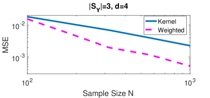
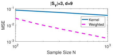
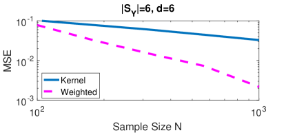
Figure 1: MSE log-log plots as a function of sample size for the uniform kernel plug-in MI estimator ("Kernel") and the proposed optimally weighted ensemble estimator $\tilde{\mathbf{G}}_{GENIE}$ ("Weighted") for the distributions described in the text. The ensemble estimator outperforms the kernel plug-in estimator, especially for larger sample sizes. Note also that as the dimension increases, the performance gap between the two estimators increases.

For the second case, $\mathbf{Y}$ has six possible outcomes (i.e. $|\mathcal{S}_{Y}|=6$) and respective probabilities $\Pr(\mathbf{Y}=0)=0.35$, $\Pr(\mathbf{Y}=1)=0.2$, $\Pr(\mathbf{Y}=2)=\Pr(\mathbf{Y}=3)=0.15$, $\Pr(\mathbf{Y}=4)=0.1$, and $\Pr(\mathbf{Y}=5)=0.05$. We chose $\alpha=0.5$ and $d=6$. The conditional covariance matrices are again $0.1\times I_{d}$ and the conditional means are, respectively, $\bar{\mu}_{0}=0.25\times\bar{1}_{d}$, $\bar{\mu}_{1}=0.75\times\bar{1}_{d}$, and $\bar{\mu}_{2}=0.5\times\bar{1}_{d}$, $\bar{\mu}_{3}=\left(0.25\times\bar{1}_{4}^{T},0.5\times\bar{1}_{2}^{T}\right)^{T}$, $\bar{\mu}_{4}=\left(0.75\times\bar{1}_{2}^{T},0.375\times\bar{1}_{4}^{T}\right)^{T}$, and $\bar{\mu}_{5}=\left(0.5\times\bar{1}_{4}^{T},0.25\times\bar{1}_{2}^{T}\right)^{T}$. The results are again given in Figure 1. The parameters for the ensemble estimator and the KDE plug-in estimators are the same as in the other three plots in Figure 1. The ensemble estimator also outperforms the plug-in estimator in this setting.

The estimated negative slopes of the log-log plots in Figure 1 are given in Table I. In all settings, both the plug-in and ensemble estimators outperform their theoretical rates in this finite-sample regime. However, the rates are generally approaching the theoretical rates as the dimension increases. It is also clear from these slopes that the ensemble estimators greatly outperform the plug-in estimators. We expect the rates to converge to the theoretical rates as the sample size increases.

Estimator	$\left|S_{Y}\right|=3,d=4$	$\left|S_{Y}\right|=3,d=6$	$\left|S_{Y}\right|=3,d=9$	$\left|S_{Y}\right|=6,d=6$
Kernel Estimator	0.90	0.59	0.32	0.49
Kernel Theoretical	0.50	0.33	0.22	0.33
Weighted Estimator	1.45	1.42	1.21	1.51
Weighted Theoretical	1	1	1	1

Table I: Negative log-log slope of the MSE for the plots in Figure 1 as a function of the sample size. The estimated values are compared to the theoretical values. While the estimators outperform the theoretical rates in this finite sample regime, the estimator rates generally approach the theoretical rates as the dimension increases.

VI-B Application to Single-Cell RNA-Sequencing Data

A common application of MI estimation is to measure the strength of relationships between different variables, especially in a feature selection setting. Model aggregation, which includes ensemble methods, for model selection is a classical problem in statistics [86, 87, 88]. Here we use the GENIE estimator on two different single-cell RNA-sequencing (scRNA-seq) datasets to demonstrate the estimator’s utility for feature selection.

Information theory has been used previously in many genomics applications [37, 89, 90, 91, 92]. Single-cell RNA-sequencing data is obtained by measuring the RNA expression levels in individual (i.e. single) cells [93]. Thousands of genes are typically measured in thousands of cells. This allows the data to capture the heterogeneity of cell types within a sample, in contrast with bulk RNA-sequencing methods which effectively measure the average RNA expression levels within a sample. To correct for undersampling that is present in scRNA-seq data, we first performed imputation on both datasets [36].

For these datasets, we estimated two MI measures: the Rényi MI and DREMI [37]. We define the Rényi MI to be equal to the Rényi divergence between the joint distribution of $\mathbf{X}$ and $\mathbf{Y}$ and the product of the marginal distributions. The DREMI score is a weighted MI developed specifically for analyzing single-cell data [37]. See Appendix A-A for further details. Note that no other estimator has been defined for $I_{DREMI}$ when the dimension of the continuous component or components are greater than 1.

VI-B1 Mouse bone marrow data

We applied GENIE to scRNA-seq data measured from developing mouse bone marrow cells [94]. Estimating mutual information is commonly done in feature selection where features (in this case the expression levels of genes) are selected based on the estimated mutual information between the features $\mathbf{X}$ (in this case the gene expression levels) and the response variable $\mathbf{Y}$ (in this case the cell type classification). Features with higher MI are chosen as they provide more information about the response variable. After preprocessing, the data contained 10,738 genes measured in 2,730 cells. In [94], the authors assigned each of the cells to one of 19 different cell types based on its gene expression profile. Examples of cell types in this data include erythrocytes, basophils, and monocytes.

For this data, we estimated the two different MI measures between the cell type classification (discrete) and selected groups of genes (continuous). We estimated the MI for different combinations of genes selected from the Kyoto Encyclopedia of Genes and Genomes (KEGG) pathways associated with the hematopoietic cell lineage [95, 96, 97]. Each of these collections contained 8-10 genes. Since the number of cell types is discrete and the gene expression levels are continuous, the estimation problem corresponds to estimating the MI between $\mathbf{X}$ and $\mathbf{Y}$ for the case where $\mathbf{Y}$ is discrete and $\mathbf{X}$ is continuous. In this problem, $|\mathcal{S}_{Y}|=19$ and $d_{X}$ is the number of genes in the chosen collection.

Table II gives the results. The mean and standard deviation of the estimated MI (calculated from 1000 bootstrap samples) are reported for each gene collection including all genes from the four selected KEGG pathways. Note that the scores for DREMI and Rényi MI are not directly comparable due to different scaling. The estimated Rényi MI for these collections is higher than when selecting 8 genes at random. This is corroborated by classification accuracies obtained using either a linear SVM classifier or random forests: the classification accuracies using the KEGG pathways genes are significantly higher than those obtained using a random set of genes. This suggests the genes in KEGG pathways associated with the hematopoietic lineage do provide some information about cell type in this data. Additionally, the combined genes from all four pathways have the largest estimated MI for both measures and classification accuracy, which is expected as genes from different pathways contain information about different cell types and are thus necessary for distinguishing between cell types.

In general, the estimated DREMI when using the KEGG pathways is higher than the estimated DREMI obtained using random genes. However, several of these scores are within a standard deviation of the score obtained from the random genes. Of the four KEGG pathways collections, the Erythrocyte pathway genes has the largest estimated Rényi MI and smallest estimated DREMI. Yet, the classification accuracy is essentially the same as that of the Platelets pathway geneset. These results highlight the different use cases of these two MI measures. The Erythrocyte cells are the largest group, containing 1,095 cells. This suggests that the estimated Rényi MI is biased high for features relevant for overrepresented groups. In contrast, the DREMI score appears to be biased low in this case. These results indicate that the DREMI score may be more appropriate than the Rényi MI when analyzing less common populations. On the other hand, when less common populations are not relevant to the analysis, DREMI may not be as appropriate as other MI measures. These different use cases highlight the utility of the GENIE estimator in estimating different MI measures.

	Platelets	Erythrocytes	Neutrophils	Macrophages	Combined	Random
Estimated Rényi MI	$0.24\pm 0.11$	$0.66\pm 0.11$	$0.27\pm 0.10$	$0.15\pm 0.09$	$1.65\pm 0.36$	$0.007\pm 0.07$
Estimated DREMI	$0.25\pm 0.22$	$0.04\pm 0.03$	$0.20\pm 0.12$	$0.41\pm 0.45$	$0.88\pm 0.35$	$0.03\pm 0.08$
SVM Accuracy	57.4%	57.5%	52.9%	52.9%	65.4%	43.2%
Random Forests Accuracy	60.3%	60.0%	57.8%	57.8%	65.9%	52.3%

Table II: Estimated Rényi MI and DREMI between collections of genes and cell type for mouse bone marrow scRNA-seq data [94] and the corresponding classification accuracies from a linear support vector machine and random forests using 10-fold cross validation. Gene collections are selected from the KEGG pathways associated with the hematopoietic cell lineage. The fifth column (with heading “Combined”) gives the result when combining all genes together from the four KEGG pathways. The last column gives the results when selecting 8 genes at random averaged over 50 trials. MI results are presented in the form of mean $\pm$ standard deviation which are calculated from 1000 bootstrapped samples.

VI-B2 Human embryoid body data

We applied GENIE to scRNA-seq data measured from human embryoid bodies (EB) collected over a 27-day time course [38]. Cells were sampled at 3-day intervals and then pooled resulting in 5 different sample collections over time. Thus sample 1 contains cells from days 0 and 3, sample 2 contains cells from days 6 and 9, etc. After preprocessing, the data contained 17,580 genes measured in 16,825 cells, with each of the five time samples containing about 2,400 to 4,100 cells. In [38], the authors identified and analyzed several branches of cells. We used GENIE to identify genes associated with a neural progenitor (NP) branch and a neural crest (NC) branch by estimating the Rényi MI and the DREMI score between the gene expression levels of the cells in each branch ($\mathbf{X}$) and the timecourse variable ($\mathbf{Y}$). This again corresponds to the case where $\mathbf{Y}$ is discrete and $\mathbf{X}$ is continuous. For this problem, $|\mathcal{S}_{Y}|=5$ and $d_{X}$ is allowed to vary as described below. Figure 2 shows PHATE visualizations of the data highlighted by time sample, and the two branches.

Figure 2: PHATE visualizations of the EB scRNA-seq data from [38] colored by time sample (left), a neural progenitors branch (middle), and a neural crest branch (right).

We performed three experiments with each of the branches. For all experiments, we limited ourselves to genes that are on average nondecreasing in the branch as time goes on. Thus in each branch, we only considered the genes such that the correlation between the gene expression level and time is greater than zero.

For the first experiment, we estimated the MI scores between the time course variable and a single gene for all genes in the data (i.e., $d_{X}=1$). Table III contains the estimated MI scores of the top 10 genes for each of the measures and branches. Several of these genes are known to be associated with their respective tissues. For example, CX3CL1 is often expressed in the brain [98], SEPT6 has been found to be important for the developing neural tube in zebra fish [99], SREBF2 is necessary for normal brain development in mice [100], NR2E1 is predominantly expressed in the developing brain [101], and ZNF804A may help regulate early brain development [102]. For the NC branch, multiple HOX genes are listed as having high Rény MI, all of which are known to be important in the NC [103]. Additionally, RBP1 has been found in enteric nerve NC cells [104], SHC4 is involved in melanocyte (an NC derivative) development [105], and PRAME is involved in further differentiation of NC cells [106].

Neural Progenitors Branch						Neural Crest Branch
Rényi MI		DREMI		SIS		Rényi MI		DREMI		SIS
LINC00526	1.004	BRWD1-AS2	8.768	FOS	0.934	HOXB7	0.837	CRYL1	10.324	RARB	0.918
GTF2E2	1.003	NR2E1	8.579	GTF2E2	0.934	SEPT6	0.820	SHC4	9.890	DDIT4	0.917
SEPT6	0.966	ZNF804A	8.505	SLC18B1	0.932	HOXA3	0.818	SLITRK2	9.692	HOXB7	0.909
SREBF2	0.963	SYT4	8.233	JAM2	0.931	HOXA7	0.818	GDNF-AS1	9.304	RGCC	0.908
EFCAB1	0.948	NTNG1	8.146	EGR1	0.930	RBP1	0.806	PRAME	9.235	IGFBP7	0.905
RP11-68606.2	0.937	GPR1	8.001	CX3CL1	0.929	ACADS	0.804	PAQR6	9.164	HOXA5	0.904
B2M	0.936	POU3F4	7.899	MAGEL2	0.927	HOXB5	0.803	Clorf198	9.044	AEBP1	0.903
CX3CL1	0.928	HSD17B8	7.704	LINC00632	0.927	HOXB6	0.794	HSPB2	8.971	HOXA7	0.901
RP3-525N10.2	0.928	LINC00092	7.686	TPPP3	0.927	HOXB3	0.793	LINC00518	8.904	ACADS	0.901
C20orf96	0.926	WNT4	7.685	GSTM3	0.927	RND3	0.791	AZGP1	8.890	PPP1R15A	0.900

Table III: Results when computing the Rényi MI, DREMI, and the SIS between the time course variable and a single gene (i.e. $d_{X}=1$) for all genes in the data with nonnegative correlations with time. The top 10 genes for each branch and score are shown here. The SIS score corresponds to the correlation coefficient. Many of the genes are known to be associated with their respective tissues.

For comparison, we also used the sure independence screening (SIS) approach described in [107]. This approach reduces to selecting the genes with the largest correlation with $\mathbf{Y}$. Table III shows the top 10 genes for each of the branches and the corresponding correlation coefficient. Note that only 1/10 of the SIS-selected genes match with the Rényi MI-selected genes in the NP branch and only 3/10 in the NC branch. None of the DREMI-selected genes match the SIS-selected genes. Since the SIS approach focuses on linear relationships, this suggests that our MI estimator is able to effectively detect strong relationships that are not strictly linear.

None of the DREMI-selected genes match the Rényi MI-selected genes in both branches. Visualizing the gene expression levels of the selected genes using PHATE indicates that genes with high DREMI scores tend to be more localized to a branch while genes with high Rényi MI may be spread out more (see Figure 3 for some examples). This suggests that the DREMI score may be better than the Rényi MI when the goal is to identify genes that are uniquely expressed in specific branches. Again, these different use cases highlight the utility of the GENIE estimator in estimating different MI measures.

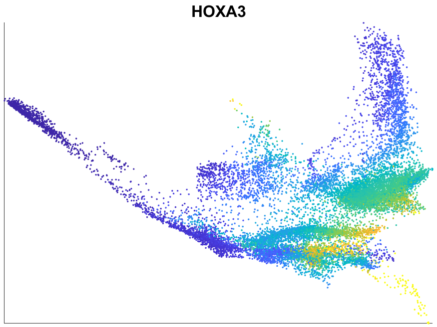
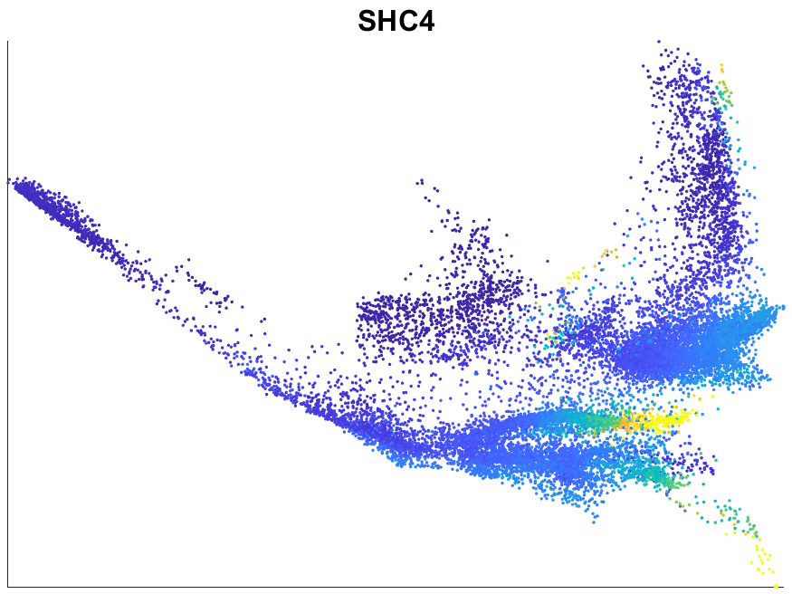
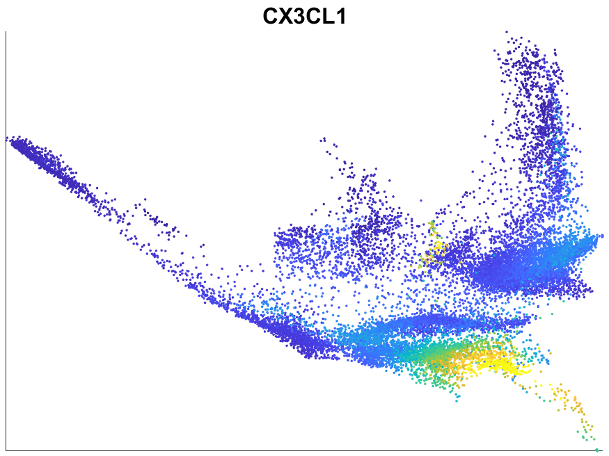
Figure 3: PHATE visualization colored by gene expression levels with genes selected as relevant for a given branch based on the estimated Rényi MI or DREMI (see Table III). These genes showcase differences in the two MI measures. Genes with high DREMI scores tend to be more localized to a branch while genes with high Rényi MI may be spread out more.

For the second experiment, we used a greedy forward-selection approach with the GENIE estimator to identify relevant genes for the two branches. For the third experiment, we used the same forward-selection approach as in the second experiment except we started by including three or four relevant genes identified in [38] per branch. In these experiments, we were able to identify several genes with known associations with these cell types. See Appendix A-B for details.

Our results here indicate that GENIE can be useful in identifying relevant features under multiple settings, even when the variables are not purely continuous or purely discrete. In particular, since GENIE accurately identifies previously known gene relationships, we propose that GENIE can be used to identify unknown gene relationships for biological discovery. This use can also be extended to other domains for scientific discovery.

VII Conclusion

We derived the MSE convergence rates for general plug-in KDE-based estimators of general MI measures between $\mathbf{X}$ and $\mathbf{Y}$ when they have only continuous components and for the case where $\mathbf{X}$ and/or $\mathbf{Y}$ contain a mixture of discrete and continuous components. Using these rates, we defined an ensemble estimator GENIE that achieves an MSE rate of $O(1/N)$ when the densities are sufficiently smooth. To the best of our knowledge, this is the first nonparametric MI estimator that achieves the MSE convergence rate of $O(1/N)$ in this setting of mixed random variables (i.e. $\mathbf{X}$ and $\mathbf{Y}$ are not both purely discrete or purely continuous). We also derived a minimax lower bound on the convergence rate for estimating MI in the continuous case, derived the asymptotic distribution of the estimator, validated the superior convergence rate of the ensemble estimator via experiments, and applied the estimator to analyze feature relevance in single cell data. We show that the ensemble estimators for the continuous case achieve the minimax rate for sufficiently smooth densities. Future work includes extending this approach to $k$-nn based estimators which are generally computationally easier than KDE estimators and extending the minimax rate for the mixed case considered here. We conjecture that the minimax rates in the mixed case are at least as slow as those for the continuous case as the mixed case can be decomposed into a random sum of continuous MI estimators.

Appendix A Extended Genomics Details and Results

Here we provide further details on the genomics experiments.

A-A Imputation and DREMI

Single-cell RNA-sequencing data typically suffers from undersampling. Therefore, we perform imputation on both datasets using MAGIC [36] prior to estimating the MI measures.

Typically, MI measures are weighted by the joint probability density of $\mathbf{X}$ and $\mathbf{Y}$. In DREMI, the measure is instead weighted by the conditional probability density of $\mathbf{Y}|\mathbf{X}$. This allows DREMI to measure the strength of the relationship between $\mathbf{Y}$and $\mathbf{X}$ regardless of differences in population density that often arise in single-cell data. Since $\mathbf{X}$ is continuous and $\mathbf{Y}$ is discrete for both genomics applications, DREMI can be defined mathematically as

$$I_{DREMI}(\mathbf{X};\mathbf{Y}) =\sum_{y\in S_{Y}}\int f_{Y_{D}|X_{C}}(y|x)\log\left(\frac{f_{X_{D}Y_{C}}(x_{C},y)}{f_{X_{C}}(x_{C})f_{Y_{D}}(y)}\right)dx_{C}$$

$$=\sum_{y\in S_{Y}}f_{Y_{D}}(y)\int\log\left(\frac{f_{X_{C}|Y_{D}}\left(x_{C}|y\right)}{f_{X_{C}}\left(x_{C}\right)}\right)\frac{f_{X_{C}|Y_{D}}\left(x_{C}|y\right)}{f_{X_{C}}\left(x_{C}\right)}dx_{C}.$$

This measure differs from standard Shannon MI with the inclusion of the weight $1/f_{X_{C}}\left(x_{C}\right)$ within the integral. While this does not fit our standard definition of a generalized MI, our estimation approach allows us to include the inverse of the KDE of $f_{X_{C}}$ when estimating the integral. The proof techniques are unaffected and therefore our theoretical results still hold.

A-B EB Data Extended Results

For the second experiment, we used a greedy forward-selection approach with the GENIE estimator to identify relevant genes. We first selected the gene with the highest estimated MI in a given branch ($d_{X}=1$). We then identified the gene that gave the largest MI when included with the first gene ($d_{X}=2$). We then repeated this to obtain the top 10 genes. The results are shown in Table IV. Rényi MI should never decrease as we add more genes, and we indeed see this in Table IV. Thus the relative increase in estimated Rényi MI can be used as a measure of the amount of information each gene adds. Note that for both branches, the largest increase in Rényi MI occurs within the first four genes and the inclusion of each subsequent gene adds a decreasing amount of Rényi MI. However, several of these genes have known associations with their respective branches. Mutations of HFE are associated with neurological disorders [108] while DOC2A is mainly expressed in the brain [109]. For the NC branch, RGR is associated with eye development which comes partially from the neural crest, ITPKB is associated with neurulation [110], and DPYSL4 is associated with the development of the nervous system [111].

Neural Progenitors (NP) Branch						Neural Crest (NC) Branch
Rényi MI		DREMI		SIS		Rényi MI		DREMI		SIS
LINC00526	1.004	BRWD1-AS2	9	FOS	0.934	HOXB7	0.837	CRYL1	10	RARB	0.918
HFE	1.382	FOSL1	15	CDC37L1-AS1	0.360	AF127936.9	1.119	IDH3B	14	ID3	0.394
DOC2A	1.675	TCP11	30	SH3GL2	0.194	RGR	1.407	AC142528.1	11	ZNF564	0.282
P4HA1	1.931	BRD9	48	ATP13A3	0.229	RP11-324E6.10	2.151	CFL1	33	MALRD1	0.188
HIST1H1C	2.030	HFE	103	DARS	0.178	LIMA1	2.347	RP11-676J15.1	64	BRWD1-AS2	0.165
PRDM12	2.152	RP11-225H22.4	224	RP11-390P2.4	0.171	ITGA9	2.581	RP5-1098D14.1	87	RP11-10A14.4	0.169
ACTR3C	2.189	ATG9A	335	ZNF484	0.167	TTLL9	2.699	BMP8B	193	SLC10A5	0.126
TRDC	2.222	RP11-35015.1	848	SIDT2	0.164	ITPKB	2.826	SLITRK2	936	RP3-402G11.26	0.117
MMEL1	2.285	GAS2L3	2385	NEFH	0.140	ACOT1	2.857	TMCC	1846	ABCC1	0.122
LINC01229	2.327	PRAC1	5845	ZNF587	0.127	DPYSL4	2.869	MLANA	6201	RPSA	0.124

Table IV: Results when computing the Rényi MI, DREMI, and the SIS between the time course variable and multiple genes using a greedy forward-selection approach. The top 10 genes for each branch and score are shown here. The SIS score corresponds to the correlation coefficient of gene expression with the regression residuals. Many of these genes are known to be associated with their respective tissues.

While the Rényi MI does not decrease with the addition of genes, DREMI may decrease due to the reweighting caused by using the conditional distribution instead of the joint. Thus the change in score when adding genes is less informative for DREMI. For a fixed dimension, however, the relative DREMI scores are informative and thus can be used to identify relevant genes using the forward-selection approach. Using this approach with DREMI, we identified several genes with known associations such as HFE (also identified with Rényi MI) and BRD9 [112] with the NP branch, and CFL1 [104] and BMP8B [113] with the NC branch.

We also performed a forward-selection variant on SIS. We first selected the gene with the highest SIS score (correlation coefficient in this case). We then performed regression with this gene and the time course variable $\mathbf{Y}$. We then calculated the SIS score between all of the other genes individually and the regression residuals to select the next gene. This process was repeated to obtain a list of the top ten genes in Table IV. Since the SIS criteria is scale-invariant, this can sometimes result in an increase in the correlation coefficient as more genes are included, although generally we expect the correlation to decrease. Thus it is somewhat difficult to assess using SIS the amount of information added by including each gene. In this case, the MI and SIS approaches identified unique genes with no shared overlap in either branch, again suggesting that our MI approaches are identifying nonlinear relationships.

For the third experiment, we used the same forward-selection approach as in the second experiment except we started by including three or four relevant genes identified in [38]. These genes were NKX2-8, EN2, and SOX1 for the NP branch, and PAX3, FOXD3, SOX9, and SOX10 for the NC branch. The results are presented in Table V. Interestingly, including these “preset” genes results in a larger overall Rényi MI and DREMI in the NP branch than when using a purely greedy approach (Table IV) while the opposite is true for the NC branch. Additionally, the identified genes are all different from the purely greedy approach. However, many of them are known to be associated with their respective tissues. PTK6 affects neurite extension [114], SIRT3 regulates mitochondria in the brain during development [115], HEY1 is expressed in neural precursor cells [116], BMPR1B is important for brain development [117], FAM72C is enriched in cortical neural progenitors [118], PPFIA4 is involved in neural development [119], LRSAM1 is related to enteric NC cells [120], LINC00327 is associated with regulating neuroblasts [121], and GRHPR is associated with human eye development [122].

Neural Progenitors (NP) Branch						Neural Crest (NC) Branch
Rényi MI		DREMI		SIS		Rényi MI		DREMI		SIS
NKX2-8	-	NKX2-8	-	NKX2-8	-	PAX3	-	PAX3	-	PAX3	-
EN2	-	EN2	-	EN2	-	FOXD3	-	FOXD3	-	FOXD3	-
SOX1	-	SOX1	-	SOX1	-	SOX9	-	SOX9	-	SOX9	-
SLX1B	2.030	MSS51	15	FAM174A	0.567	SOX10	-	SOX10	-	SOX10	-
PTK6	2.613	KNSTRN	247	RAB27A	0.329	RP11-867G23.8	1.614	GRHPR	7	ARMC5	0.543
SIRT3	3.204	TEKT3	548	CTD-2568A17.1	0.321	ZBED3	1.759	LINC01389	23	ABL1	0.325
HEY1	3.596	FAM72C	1998	CECR5	0.209	RP3-460G2.2	1.830	CTB-25B13.5	50	PSPN	0.338
OLIG2	4.021	GZMK	4904	LOXL1	0.163	LRSAM1	1.855	CFAP58	68	RP11-354P11.3	0.262
MZF1-AS1	4.689	QRICH2	16337	PROB1	0.147	NOTUM	1.930	ZNF774	271	WWTR1-AS1	0.185
BMPR1B	5.133	PPFIA4	42236	YY2	0.161	CPLX2	1.945	LINC00327	588	KIF25	0.144

Table V: Results when computing the Rényi MI, DREMI, and the SIS between the time course variable and multiple genes using a greedy forward-selection approach when starting with three or four relevant genes identified in [38]. The top 10 genes for each branch and score are shown here. The SIS score corresponds to the correlation coefficient of gene expression with the regression residuals. Many of these genes are known to be associated with their respective tissues.

Appendix B MI Ensemble Estimation Extensions

In this appendix, we present several extensions of the ensemble estimation approach to MI. First, we show how to apply the theory to the purely continuous case. We then show how the theory can be applied to obtain estimators that achieve the parametric rate for less smooth densities.

B-A Continuous Random Varables

We can apply Theorem 3 in [14] to obtain a version of the GENIE MI estimator that achieves the parametric rate for the case when $\mathbf{X}$ and $\mathbf{Y}$ are purely continuous. For completeness, we repeat the theorem and its proof here. For a general estimation problem, let $N$ be the number of available samples and let $\mathcal{L}=\left\{l_{1},\dots,l_{L}\right\}$ be a set of index values. For an indexed ensemble of estimators $\left\{\hat{\mathbf{E}}_{l}\right\}_{l\in\mathcal{L}}$ of a parameter $E$, the weighted ensemble estimator with weights $w=\left\{w\left(l_{1}\right),\dots,w\left(l_{L}\right)\right\}$ satisfying $\sum_{l\in\mathcal{L}}w(l)=1$ is defined as

$$\hat{\mathbf{E}}_{w}=\sum_{l\in\mathcal{L}}w\left(l\right)\hat{\mathbf{E}}_{l}.$$

Consider the following conditions on $\left\{\hat{\mathbf{E}}_{l}\right\}_{l\in\mathcal{L}}$:

• $\mathcal{C}.1$ The bias is expressible as

  $$\mathbb{B}\left[\hat{\mathbf{E}}_{l}\right]=\sum_{i\in J}c_{i}\psi_{i}(l)\phi_{i,d}(N)+O\left(\frac{1}{\sqrt{N}}\right),$$

  where $c_{i}$ are constants depending on the underlying density and are independent of $N$ and $l$, $J=\left\{i_{1},\dots,i_{I}\right\}$ is a finite index set with $I<L$, and $\psi_{i}(l)$ are basis functions depending only on the parameter $l$ and not on the sample size $N$.

• $\mathcal{C}.2$ The variance is expressible as

  $$\mathbb{V}\left[\hat{\mathbf{E}}_{l}\right]=c_{v}\left(\frac{1}{N}\right)+o\left(\frac{1}{N}\right).$$

Theorem 11 (Theorem 3 in [14]).

Assume conditions $\mathcal{C}.1$ and $\mathcal{C}.2$ hold for an ensemble of estimators $\left\{\hat{\mathbf{E}}_{l}\right\}_{l\in\mathcal{L}}$. Then there exists a weight vector $w_{0}$ such that the MSE of the weighted ensemble estimator attains the parametric rate of convergence:

$$\mathbb{E}\left[\left(\hat{\mathbf{E}}_{w_{0}}-E\right)^{2}\right]=O\left(\frac{1}{N}\right).$$

The weight vector $w_{0}$ is the solution to the following convex optimization problem:

$$\begin{array}[]{rl}\min_{w}&||w||_{2}\\ \text{subject to}&\sum_{l\in\mathcal{L}}w(l)=1,\\ &\gamma_{w}(i)=\sum_{l\in\mathcal{L}}w(l)\psi_{i}(l)=0,\,i\in J.\end{array}$$ (31)

Proof.

Due to condition $\mathcal{C}.1$, the bias of the weighted ensemble estimator is

$$\mathbb{B}\left[\hat{\mathbf{E}}_{w}\right]=\sum_{i\in J}c_{i}\gamma_{w}(i)\phi_{i,d}(N)+O\left(\frac{\sqrt{L}||w||_{2}}{\sqrt{N}}.\right)$$ (32)

Denote the covariance matrix of the ensemble of estimators as $\Sigma_{L}$. By the Cauchy-Schwarz inequality and condition $\mathcal{C}.2$, the entries of $\Sigma_{L}$ are $O(1/N)$. The variance of the weighted estimator is then bounded above as

$$\mathbb{V}\left[\hat{\mathbf{E}}_{w}\right]=w^{T}\Sigma_{L}w\leq\frac{Trace(\Sigma_{L}N)||w||_{2}^{2}}{N}=\frac{c_{v}L||w||_{2}^{2}}{N}+o\left(\frac{1}{N}\right).$$ (33)

The optimization problem in (31) zeroes out the lower-order bias terms and limits the $\ell_{2}$ norm of the weight vector $w$ to prevent the variance from exploding. This results in an MSE of $O(1/N)$ as long as the dimension $d$ is fixed and $L$ is fixed and independent of the sample size $N$. A solution is guaranteed to (31) as long as $L>I$ and the vectors $a_{i}=[\psi_{i}(l_{1}),\dots,\psi_{i}(l_{L})]$ are linearly independent.

∎

As before, (31) typically results in an ensemble estimator with a large variance. We can relax this optimization problem and obtain an estimator that still obtains the parametric rate:

$$\begin{array}[]{rl}\min_{w}&\epsilon\\ \text{subject to}&\sum_{l\in\mathcal{L}}w(l)=1,\\ &\left|\gamma_{w}(i)N^{\frac{1}{2}}\phi_{i,d}(N)\right|\leq\epsilon,\,\,i\in J,\\ &\left\|w\right\|_{2}^{2}\leq\eta\epsilon.\end{array}$$ (34)

We can use (34) to obtain a GENIE estimator for the purely continuous case. Theorem 2 indicates that we need $h_{X}^{d_{X}}h_{Y}^{d_{Y}}\propto N^{-1/2}$ for the $O(1/(Nh_{X}^{d_{X}}h_{Y}^{d_{Y}}))$ terms to be $O(1/\sqrt{N})$. We consider the more general case where the parameters may differ for $h_{X}$ and $h_{Y}$. Let $\mathcal{L}_{X}$ and $\mathcal{L}_{Y}$ be sets of real, positive numbers with $|\mathcal{L}_{X}|=L_{X}$ and $|\mathcal{L}_{Y}|=L_{Y}$. For each estimator in the ensemble, choose $l_{X}\in\mathcal{L_{X}}$ and $l_{Y}\in\mathcal{L}_{Y}$ and set $h_{X}(l_{X})=l_{X}N^{-1/(2(d_{X}+d_{Y}))}$ and $h_{Y}(l_{Y})=l_{Y}N^{-1/(2(d_{X}+d_{Y}))}$. Define the matrix $w$ s.t. $\sum_{l_{X}\in\mathcal{L}_{X},l_{Y}\in\mathcal{L}_{Y}}w(l_{X},l_{Y})=1$. From Theorems 2 and 3, conditions $\mathcal{C}.1$ and $\mathcal{C}.2$ are satisfied if $s\geq d_{X}+d_{Y}$ with $\psi_{i,j}(l_{X},l_{Y})=l_{X}^{i}l_{Y}^{j}$ and $\phi_{i,j}(N)=N^{-(i+j)/(2(d_{X}+d_{Y}))}$ for $0\leq i,j\leq d_{X}+d_{Y}$ s.t. $0<i+j\leq d_{X}+d_{Y}$. The optimal weight $w_{0}$ is calculated using (34). The resulting estimator

$$\tilde{\mathbf{G}}_{w_{0}}^{cont}=\sum_{l_{X}\in\mathcal{L}_{X},l_{Y}\in\mathcal{L}_{Y}}w_{0}(l_{X},l_{Y})\tilde{\mathbf{G}}_{h_{X}(l_{X}),h_{Y}(l_{Y})}$$

achieves the parametric MSE rate when $s\geq d_{X}+d_{Y}$. We denote this estimator as $\tilde{\mathbf{G}}_{GENIE}^{cont}$.

B-B Less Smooth Densities

The GENIE estimators $\tilde{\mathbf{G}}_{GENIE}$ and $\tilde{\mathbf{G}}_{GENIE}^{cont}$ are guaranteed to achieve the parametric convergence rate as long as $s\geq d_{X}+d_{Y}$. Here we derive ensemble estimators of MI that achieve the parametric rate under less strict smoothness assumptions on the densities. To derive the ensemble estimators for less smooth densities, we need a different expansion of the bias that includes some higher order terms. We present those results here for the continuous and mixed cases and show how to apply the ensemble estimation theory to obtain the parametric MSE convergence rate when the densities are less smooth ($s>(d_{X}+d_{Y})/2$).

B-B1 Continuous Random Variables

We first consider the case where $\mathbf{X}$ and $\mathbf{Y}$ are both purely continuous. Consider the following result on the bias of the plug-in estimator:

Theorem 12 (Continuous Bias Expanded).

Assume that assumptions $\mathcal{A}.0$-$\mathcal{A}.5$ hold. Then for $\lambda\geq 2$ a positive integer, the bias of $\tilde{\mathbf{G}}_{h_{X},h_{Y}}$ is

$$\mathbb{B}\left[\tilde{\mathbf{G}}_{h_{X},h_{Y}}\right] = \sum_{\begin{subarray}{c}m,n=0\\ i+j+m+n\neq 0\end{subarray}}^{\lambda}\sum_{i,j=0}^{r}c_{11,i,j,m,n}\frac{h_{X}^{i}h_{Y}^{j}}{\left(Nh_{X}^{d_{X}}\right)^{m}\left(Nh_{Y}^{d_{Y}}\right)^{n}}$$ (35)

$$+\sum_{m=1}^{\lambda}\sum_{i=0}^{r}\sum_{j=0}^{r}c_{13,i,j,m}h_{X}^{i}h_{Y}^{j}/\left(Nh_{X}^{d_{X}}h_{Y}^{d_{Y}}\right)^{m}$$

$$+O\left(h_{X}^{s}+h_{Y}^{s}+1/\left(Nh_{X}^{d_{X}}h_{Y}^{d_{Y}}\right)^{\lambda}\right).$$

The proof is given in Appendix D. Note that no extra assumptions are required to achieve this result compared to Theorem 2. However, we elected to retain these results for the appendix to simplify the presentation in the main paper.

We now use these results to define a new ensemble estimator. Set $\delta>0$ and let $\mathcal{L}_{X}$ and $\mathcal{L}_{Y}$ be sets of real, positive numbers with $|\mathcal{L}_{X}|=L_{X}$ and $|\mathcal{L}_{Y}|=L_{Y}$. For each estimator in the ensemble, choose $l_{X}\in\mathcal{L_{X}}$ and $l_{Y}\in\mathcal{L}_{Y}$ and set $h_{X}(l_{X})=l_{X}N^{-1/(d_{X}+d_{Y}+\delta)}$ and $h_{Y}(l_{Y})=l_{Y}N^{-1/(d_{X}+d_{Y}+\delta)}$. Then conditions $\mathcal{C}.1$ and $\mathcal{C}.2$ are satisfied if $s\geq(d_{X}+d_{Y}+\delta)/2$ and $\lambda\geq(d_{X}+d_{Y}+\delta)/\delta$ with $\psi_{1,i,j,m,n}(l_{X},l_{Y})=l_{X}^{i-md_{X}}l_{Y}^{j-nd_{Y}}$ and $\phi_{1,i,j,m,n}(N)=N^{-\frac{i+j+m(d_{Y}+\delta)+n(d_{X}+\delta)}{d_{X}+d_{Y}+\delta}}$ for $0<i+j+m(d_{Y}+\delta)+n(d_{X}+\delta)\leq\frac{d_{X}+d_{Y}+\delta}{2}$ and the terms $\psi_{2,i,j,m}(l_{X},l_{Y})=l_{X}^{i-md_{X}}l_{Y}^{j-md_{Y}}$ and $\phi_{2,i,j,m}(N)=N^{-\frac{i+j+m\delta}{d_{X}+d_{Y}+\delta}}$ for $m\geq 1$ and $i+j+m\delta\leq\frac{d_{X}+d_{Y}+\delta}{2}.$ These all correspond to terms that converge to zero slower than $N^{-1/2}$ when left uncorrected. The optimal weight $w_{0}$ is again calculated using (34) and the resulting ensemble estimator achieves the parametric MSE convergence rate when $s\geq(d_{X}+d_{Y}+\delta)/2$. Since $\delta$ can be chosen arbitrarily close to zero, the parametric rate can be achieved theoretically as long as $s>(d_{X}+d_{Y})/2$.

B-B2 Mixed Random Variables

We now consider the case where $\mathbf{X}$ and $\mathbf{Y}$ may have any mixture of continuous and discrete components. We have a similar result on the bias as in Theorem 12. Here we assume that $\mathbf{h}_{X_{C}|x}=l_{X}\mathbf{N}_{x}^{-\beta}$ and $\mathbf{h}_{Y_{C}|y}=l_{Y}\mathbf{N}_{y}^{-\alpha}$ with $0<\beta<\frac{1}{d_{X}}$, $0<\alpha<\frac{1}{d_{Y}}$, and $l_{X},l_{Y}>0$.

Theorem 13 (Mixed Bias Expanded).

Assume that the same assumptions hold as in Theorem 6. Then for $\lambda\geq 2$ a positive integer, the bias of $\tilde{\mathbf{G}}_{h_{X_{C}|X_{D}},h_{Y_{C}|Y_{D}}}$ is

$$\mathbb{B}\left[\tilde{\mathbf{G}}_{h_{X_{C}|X_{D}},h_{Y_{C}|Y_{D}}}\right] =\sum_{\begin{subarray}{c}m,n=0\\ i+j+m+n\neq 0\end{subarray}}^{\lambda}\sum_{i,j=0}^{r}c_{14,i,j,m,n}\frac{l_{X}^{i}l_{Y}^{j}N^{-i\beta-j\alpha}}{\left(l_{X}^{d_{X}}N^{1-\beta d_{X}}\right)^{m}\left(l_{Y}^{d_{Y}}N^{1-\alpha d_{Y}}\right)^{n}}$$

$$+\sum_{m=1}^{\lambda}\sum_{i=0}^{r}\sum_{j=0}^{r}c_{15,i,j,m}\frac{l_{X}^{i}l_{Y}^{j}N^{-i\beta-j\alpha}}{\left(l_{X}^{d_{X}}l_{Y}^{d_{Y}}N^{1-\beta d_{X}-\alpha d_{Y}}\right)^{m}}$$

$$+O\left(N^{-s\beta}+N^{-s\alpha}+\frac{1}{\left(N^{1-\beta d_{X}-\alpha d_{Y}}\right)^{\lambda}}\right).$$ (36)

The proof is given in Appendix G-B.

We now use these results to define a new ensemble estimator in the mixed case. The procedure is similar to the continuous case. Set $\delta>0$ and let $\mathcal{L}_{X}$ and $\mathcal{L}_{Y}$ be sets of real, positive numbers with $|\mathcal{L}_{X}|=L_{X}$ and $|\mathcal{L}_{Y}|=L_{Y}$. For each estimator in the ensemble, choose $l_{X}\in\mathcal{L_{X}}$ and $l_{Y}\in\mathcal{L}_{Y}$ and set $\mathbf{h}_{X_{C}|x}(l_{X})=l_{X}\mathbf{N}_{x}^{-1/(d_{X}+d_{Y}+\delta)}$ and $\mathbf{h}_{Y_{C}|y}(l_{Y})=l_{Y}\mathbf{N}_{y}^{-1/(d_{X}+d_{Y}+\delta)}$. Conditions $\mathcal{C}.1$ and $\mathcal{C}.2$ are satisfied if $s\geq(d_{X}+d_{Y}+\delta)/2$ and $\lambda\geq(d_{X}+d_{Y}+\delta)/\delta$. The first set of terms in the optimization problem are $\psi_{1,i,j,m,n}(l_{X},l_{Y})=l_{X}^{i-md_{X}}l_{Y}^{j-nd_{Y}}$ and $\phi_{1,i,j,m,n}(N)=N^{-\frac{i+j+m(d_{Y}+\delta)+n(d_{X}+\delta)}{d_{X}+d_{Y}+\delta}}$ for $0<i+j+m(d_{Y}+\delta)+n(d_{X}+\delta)\leq\frac{d_{X}+d_{Y}+\delta}{2}$. The second set of terms are $\psi_{2,i,j,m}(l_{X},l_{Y})=l_{X}^{i-md_{X}}l_{Y}^{j-md_{Y}}$ and $\phi_{2,i,j,m}(N)=N^{-\frac{i+j+m\delta}{d_{X}+d_{Y}+\delta}}$ for $m\geq 1$ and $i+j+m\delta\leq\frac{d_{X}+d_{Y}+\delta}{2}.$ The optimal weight $w_{0}$ is again calculated using (34) and the resulting ensemble estimator achieves the parametric MSE convergence rate when $s\geq(d_{X}+d_{Y}+\delta)/2$. Since $\delta$ can be chosen arbitrarily close to zero, the parametric rate can be achieved theoretically as long as $s>(d_{X}+d_{Y})/2$.

The modified estimators defined in this section have better statistical properties than the original GENIE estimators defined in Section V and Appendix B-A as the parametric rate is guaranteed under less restrictive smoothness assumptions on the densities. On the other hand, the number of parameters required for the optimization problem in (34) is larger for the modified estimator. In theory, this could lead to larger variance although this is not necessarily true in practice according to divergence estimation experiments in [72].

Appendix C The Boundary Condition

Here we prove that under certain smoothness assumptions on a kernel with either rectangular or circular support, the boundary assumption $\mathcal{A}.5$ is satisfied for densities with the unit cube as its support set. We will prove the following, more general result:

Theorem 14.

Let $K$ be a kernel function with rectangular or circular support, i.e., $K(u)=0$ for $\left\|u\right\|_{1}>1$ or $\left\|u\right\|_{2}>1$, respectively. Let $K\in\Sigma(s,H_{K})$ in the interior of its support. Let $p_{x}(u):\mathbb{R}^{d}\rightarrow\mathbb{R}$ be a polynomial in $u$ of order $|q|\leq r=\left\lfloor s\right\rfloor$ whose coefficients are a function of $x$ and are $r-|q|$ times differentiable. Then for $\mathcal{S}=[0,1]^{d}$ and any positive integers $t$ and $m$, we have that

$$\int_{x\in\mathcal{S}}\left(\int_{u:K(u)>0,\,x+uh\notin\mathcal{S}}K^{l}(u)p_{x}(u)du\right)^{t}dx=v_{t}(h),$$ (37)

where $v_{t}(h)$ admits the expansion

$$v_{t}(h)=\sum_{i=1}^{r-|q|}e_{i,q,t,l}h^{i}+o\left(h^{r-q}\right),$$

for some constants $e_{i,q,t,l}$.

Before proving this, we will relate this result to assumption $\mathcal{A}.5$.

Corollary 15.

Assumption $\mathcal{A}.5$ is satisfied under the same conditions as in Theorem 14, i.e., $K\in\Sigma(s,H_{K})$ is a kernel function with either rectangular or circular support and $\mathcal{S}=[0,1]^{d}$.

This follows immediately from assumption $\mathcal{A}.2$ that $f$ is in the Hölder class $\Sigma(s,H)$, which implies that $D^{q}f(x)$ is $r-|q|$ times differentiable. Thus equation (37) implies $\mathcal{A}.5$.

C-A Proof of Theorem 14: Rectangular Support Kernels

We will first consider points that are boundary points due to a single coordinate and then extend to the general case where multiple coordinates are close to the boundary.

Single Coordinate Boundary Point

Since $K\in\Sigma(s,H_{K})$, we can take a Taylor series expansion of $K^{l}(u)$ around zero to obtain

$$K^{l}(u)=p_{K,l}(u)+o(||u||_{2}^{r}),$$ (38)

where $p_{K,l}(u)$ is a polynomial function of $u$ with degree $r$.

Consider points $x$ that are boundary points by virtue of a single coordinate $x_{i}$ such that $x_{i}+u_{i}h\notin\mathcal{S}$. Without loss of generality, assume that $x_{i}+u_{i}h>1$. After performing the above Taylor series expansion of $K^{l}$, the inner integral in (37) can then be evaluated first with respect to all coordinates other than $i$. Since all of these coordinates lie within the support, the inner integral over these coordinates will amount to integration of the polynomial $p_{x}(u)$ over a symmetric $d-1$ dimensional rectangular region $\left|u_{j}\right|\leq 1$ for all $j\neq i$. This yields a function $\sum_{m=1}^{q+r}\tilde{p}_{m}(x)u_{i}^{m}+o(u_{i}^{r+1})$ where the coefficients $\tilde{p}_{m}(x)$ are each $r-|q|$ times differentiable wrt $x$.

With respect to the $u_{i}$ coordinate, the inner integral will have limits from $\frac{1-x_{i}}{h}$ to $1$ for some $1>x_{i}>1-h$. Consider the $\tilde{p}_{m}(x)u_{i}^{m}$ monomial term. The inner integral wrt this term yields (ignoring the $o(\cdot)$ term for now)

$$\sum_{m=1}^{|q|+r}\tilde{p}_{m}(x)\int_{\frac{1-x_{i}}{h}}^{1}u_{i}^{m}du_{i}=\sum_{m=1}^{|q|+r}\tilde{p}_{m}(x)\frac{1}{m+1}\left(1-\left(\frac{1-x_{i}}{h}\right)^{m+1}\right).$$ (39)

Raising the right hand side of (39) to the power of $t$ results in an expression of the form

$$\sum_{j=0}^{(|q|+r)t}\check{p}_{j}(x)\left(\frac{1-x_{i}}{h}\right)^{j},$$ (40)

where the coefficients $\check{p}_{j}(x)$ are $r-|q|$ times differentiable wrt $x$. Integrating (40) over all the coordinates in $x$ other than $x_{i}$ results in an expression of the form

$$\sum_{j=0}^{(|q|+r)t}\bar{p}_{j}(x_{i})\left(\frac{1-x_{i}}{h}\right)^{j},$$ (41)

where again the coefficients $\bar{p}_{j}(x_{i})$ are $r-|q|$ times differentiable wrt $x_{i}$. Note that since the other cooordinates of $x$ other than $x_{i}$ are far away from the boundary, the coefficients $\bar{p}_{j}(x_{i})$ are independent of $h$. To evaluate the integral of (41), consider the $r-|q|$ term Taylor series expansion of $\bar{p}_{j}(x_{i})$ around $x_{i}=1$, where we use a smooth extension of the function and its derivatives to the boundary. This will yield terms of the form

$$\int_{1-h}^{1}\frac{\left(1-x_{i}\right)^{j+k}}{h^{k}}dx_{i} = \left.-\frac{\left(1-x_{i}\right)^{j+k+1}}{h^{k}(j+k+1)}\right|_{x_{i}=1-h}^{x_{i}=1}$$ (42)

$$= \frac{h^{j+1}}{(j+k+1)},$$ (43)

for $0\leq j\leq r-|q|$, and $0\leq k\leq(|q|+r)t$. By a similar analysis, the $o(\cdot)$ terms from the Taylor expansion of the kernel result in $o(h^{r})$. Combining terms results in the expansion $v_{t}(h)=\sum_{i=1}^{r-|q|}e_{i,q,t}h^{i}+o\left(h^{r-|q|}\right)$.

Multiple Coordinate Boundary Point

The case where multiple coordinates of the point $x$ are near the boundary is a straightforward extension of the single boundary point case so we only sketch the main ideas here. As an example, consider the case where 2 of the coordinates are near the boundary. Assume for notational ease that they are $x_{1}$ and $x_{2}$ and that $x_{1}+u_{1}h>1$ and $x_{2}+u_{2}h>1$. The inner integral in (37) can again be evaluated first wrt all coordinates other than 1 and 2. This yields a function $\sum_{m,j=1}^{q+r}\tilde{p}_{m,j}(x)u_{1}^{m}u_{2}^{j}$ where the coefficients $\tilde{p}_{m,j}(x)$ are each $r-q$ times differentiable wrt $x$. Integrating this wrt $x_{1}$ and $x_{2}$ and then raising the result to the power of $t$ yields a double sum similar to (40). Integrating this over all the coordinates in $x$ other than $x_{1}$ and $x_{2}$ gives a double sum similar to (41). Then a Taylor series expansion of the coefficients and integration over $x_{1}$ and $x_{2}$ yields the result.

C-B Proof of Theorem 14: Circular Support Kernels

The case where the kernel $K$ has a circular support is more complex than when the support is rectangular. We will again first consider points that are boundary points due to a single coordinate. We will then extend to the general case where multiple coordinates are close to the boundary.

Single Coordinate Boundary Point

Consider points $x$ that are boundary points due to a single coordinate $x_{i}$ s.t. $x_{i}+u_{i}h\notin\mathcal{S}$. Without loss of generality, assume that $x_{i}+u_{i}h>1$. We focus first on the inner integral in (37). We will use the following lemma:

Lemma 16.

Let $D_{d}(\rho)$ be a $d$-sphere with radius $\rho$ and let $\sum_{i=1}^{d}n_{i}=q$. Then

$$\int_{D_{d}(\rho)}u_{1}^{n_{1}}u_{2}^{n_{2}}\dots u_{d}^{n_{d}}du_{1}\dots du_{d}=C\rho^{d+q},$$

where $C$ is a constant that depends on the $n_{i}$s and $d$.

Proof.

We convert to $d$-dimensional spherical coordinates to handle the integration. Let $r$ be the distance of a point $u$ from the origin. We nave $d-1$ angular coordinates $\phi_{i}$ where $\phi_{d-1}$ ranges from $0$ to $2\pi$ and all other $\phi_{i}$ range from $0$ to $\pi$. The conversion from the spherical coordinates to Cartesian coordinates is then

$$u_{1} = r\cos\left(\phi_{1}\right)$$

$$u_{2} = r\sin\left(\phi_{1}\right)\cos\left(\phi_{2}\right)$$

$$u_{3} = r\sin\left(\phi_{1}\right)\sin\left(\phi_{2}\right)\cos\left(\phi_{3}\right)$$

$$\vdots$$

$$u_{d-1} = r\sin\left(\phi_{1}\right)\cdots\sin\left(\phi_{d-2}\right)\cos\left(\phi_{d-1}\right)$$

$$u_{d} = r\sin\left(\phi_{1}\right)\cdots\sin\left(\phi_{d-2}\right)\sin\left(\phi_{d-1}\right).$$

The spherical volume element is then

$$r^{d-1}\sin^{d-2}\left(\phi_{1}\right)\sin^{d-3}\left(\phi_{1}\right)\cdots\sin\left(\phi_{d-1}\right)dr\,d\phi_{1}\,d\phi_{2}\cdots d\phi_{d-1}.$$

Combining these results gives

$$\int_{D_{d}(\rho)}u_{1}^{n_{1}}u_{2}^{n_{2}}\dots u_{d}^{n_{d}}du_{1}\dots du_{d}$$

$$= \int_{0}^{\rho}\int_{o}^{2\pi}\int_{0}^{\pi}\cdots\int_{0}^{\pi}r^{q+d-1}\left[\sin^{q-n_{1}+d-2}\left(\phi_{1}\right)\sin^{q-n_{1}-n_{d}+d-3}\left(\phi_{2}\right)\cdots\right.$$

$$\left.\sin^{n_{d}+n_{d-1}+1}\left(\phi_{d-2}\right)\sin^{n_{d}}\left(\phi_{d-1}\right)\right]\left[\cos^{n_{1}}\left(\phi_{1}\right)\cdots\cos^{n_{d}}\left(\phi_{d-1}\right)\right]d\phi_{1}\cdots d\phi_{d-1}dr$$

$$= C\rho^{q+d}.$$

∎

Since $K\in\Sigma(s,H_{K})$, we can take a Taylor series expansion of $K^{l}(u)$ around zero to obtain

$$K^{l}(u)=p_{K,l}(u)+o(||u||_{2}^{r}),$$ (44)

where $p_{K,l}(u)$ is a polynomial function of $u$ with degree $r$.

The region of integration for the inner integral in (37) corresponds to a hyperspherical cap with radius $1$ and height of $\frac{1-x_{i}}{h}$. The inner integral can be calculated using an approach similar to that used in [123] to calculate the volume of a hyperspherical cap. It is obtained by integrating the polynomial $p_{x}(u)$ over a $d-1$-sphere with radius $\sin\theta$ and height element $d\cos\theta$. This is done using Lemma 16. We then integrate over $\theta$ which has a range of $0$ to $\phi=\cos^{-1}\left(\frac{1-x_{i}}{h}\right).$ Thus we have

$$\int_{u:x+uh\notin\mathcal{S}}K^{l}(u)p_{x}(u)du = \int_{u:||u||_{2}\leq 1,x+uh\notin\mathcal{S}}\left(p_{K,l}(u)+o(||u||_{2}^{r})\right)p_{x}(u)du$$ (45)

$$= \sum_{m=0}^{|q|+r}\tilde{p}_{m,l}(x)\int_{0}^{\phi}\sin^{m+d-1}(\theta)\sin\theta\cos^{m}\theta d\theta+o\left(\int_{u:||u||_{2}\leq 1,x+uh\notin\mathcal{S}}||u||_{2}^{r}du\right)$$

$$= \sum_{m=0}^{|q|+r}\tilde{p}_{m,l}(x)\int_{0}^{\phi}\sin^{m+d}(\theta)\cos^{m}\theta d\theta+o\left(\int_{u:||u||_{2}\leq 1,x+uh\notin\mathcal{S}}||u||_{2}^{r}du\right),$$

where $\tilde{p}_{m}(x)$ is the polynomial coefficient corresponding to $u_{i}^{m}$ after the Taylor series expansion of $K^{l}$ and integrating over the $d-1$-sphere.

We will focus on the first term in Eq. 45 as the $o(\cdot)$ term will follow similarly as a polynomial function of $u$. From standard integral tables, we get that for $n\geq 2$ and $m\geq 0$

$$\int_{0}^{\phi}\sin^{n}\theta\cos^{m}\theta d\theta=-\frac{\sin^{n-1}\phi\cos^{m+1}\phi}{n+m}+\frac{n-1}{n+m}\int_{0}^{\phi}\sin^{n-2}\theta\cos^{m}\theta d\theta.$$ (46)

If $n=1$, then we get

$$\int_{0}^{\phi}\sin\theta\cos^{m}\theta d\theta=\frac{1}{m+1}-\frac{\cos^{m+1}\phi}{m+1}.$$

Since $\phi=\cos^{-1}\left(\frac{1-x_{i}}{h}\right)$, we have

$$\cos\phi = \frac{1-x_{i}}{h},$$

$$\sin\phi = \sqrt{1-\left(\frac{1-x_{i}}{h}\right)^{2}}.$$

Therefore, if $n$ is odd, we obtain

$$\int_{0}^{\phi}\sin^{n}\theta\cos^{m}\theta d\theta=\sum_{\ell=0}^{(n-1)/2}c_{\ell}\left(\sqrt{1-\left(\frac{1-x_{i}}{h}\right)^{2}}\right)^{2\ell}\left(\frac{1-x_{i}}{h}\right)^{m+1}+c,$$ (47)

where the constants depend on $m$ and $n$.

If $n$ is even and $m>0$, then the final term in the recursion in (46) reduces to

$$\int_{0}^{\phi}\cos^{m}\theta d\theta=\frac{\cos^{m-1}\phi\sin\phi}{m}+\frac{m-1}{m}\int_{0}^{\phi}\cos^{m-2}\theta d\theta.$$

If $m=2$, then

$$\int_{0}^{\phi}\cos^{2}\theta d\theta = \frac{\phi}{2}+\frac{1}{4}\sin(2\phi)$$

$$= \frac{\phi}{2}+\frac{1}{2}\sin\phi\cos\phi.$$

Therefore, if $n$ and $m$ are both even, then this gives

$$\int_{0}^{\phi}\sin^{n}\theta\cos^{m}\theta d\theta = \sum_{\ell=0}^{(n-2)/2}c_{\ell}^{{}^{\prime}}\left(\sqrt{1-\left(\frac{1-x_{i}}{h}\right)^{2}}\right)^{2\ell+1}\left(\frac{1-x_{i}}{h}\right)^{m+1}+c^{{}^{\prime}}\cos^{-1}\left(\frac{1-x_{i}}{h}\right)$$ (48)

$$+\sum_{\ell=0}^{(m-2)/2}c_{\ell}^{{}^{\prime\prime}}\left(\sqrt{1-\left(\frac{1-x_{i}}{h}\right)^{2}}\right)\left(\frac{1-x_{i}}{h}\right)^{2\ell+1}.$$

On the other hand, if $n$ is even and $m$ is odd, we get

$$\int_{0}^{\phi}\sin^{n}\theta\cos^{m}\theta d\theta = \sum_{\ell=0}^{(n-2)/2}c_{\ell}^{{}^{\prime\prime\prime}}\left(\sqrt{1-\left(\frac{1-x_{i}}{h}\right)^{2}}\right)^{2\ell+1}\left(\frac{1-x_{i}}{h}\right)^{m+1}$$ (49)

$$+\sum_{\ell=0}^{(m-1)/2}c_{\ell}^{{}^{\prime\prime\prime\prime}}\left(\sqrt{1-\left(\frac{1-x_{i}}{h}\right)^{2}}\right)\left(\frac{1-x_{i}}{h}\right)^{2\ell}.$$

If $d$ is odd, then combining (47) and (49) with (45) gives

$$\sum_{m=0}^{|q|+r}\tilde{p}_{m,l}(x)\int_{0}^{\phi}\sin^{m+d}(\theta)\cos^{m}\theta d\theta=\sum_{m=0}^{|q|+r}\sum_{\ell=0}^{d+|q|}p_{m,\ell,l}(x)\left(\sqrt{1-\left(\frac{1-x_{i}}{h}\right)^{2}}\right)^{\ell}\left(\frac{1-x_{i}}{h}\right)^{m},$$ (50)

where the coefficients $p_{m,\ell,l}(x)$ are $r-|q|$ times differentiable wrt $x$. Similarly, if $d$ is even, then

$$\sum_{m=0}^{|q|+r}\tilde{p}_{m,l}(x)\int_{0}^{\phi}\sin^{m+d}(\theta)\cos^{m}\theta d\theta = \sum_{m=0}^{|q|+r}\sum_{\ell=0}^{d+|q|}p_{m,\ell,l}^{{}^{\prime}}(x)\left(\sqrt{1-\left(\frac{1-x_{i}}{h}\right)^{2}}\right)^{\ell}\left(\frac{1-x_{i}}{h}\right)^{m}$$ (51)

$$+p^{{}^{\prime}}(x)\cos^{-1}\left(\frac{1-x_{i}}{h}\right),$$

where again the coefficients $p_{m,\ell,l}^{{}^{\prime}}(x)$ and $p^{{}^{\prime}}(x)$ are $r-q$ times differentiable wrt $x$. Raising (50) and (51) to the power of $t$ gives respective expressions of the form

$$\sum_{m=0}^{(|q|+r)t}\sum_{\ell=0}^{(d+|q|)t}\check{p}_{m,\ell,l}(x)\left(\sqrt{1-\left(\frac{1-x_{i}}{h}\right)^{2}}\right)^{\ell}\left(\frac{1-x_{i}}{h}\right)^{m},$$ (52)

$$\sum_{m=0}^{(|q|+r)t}\sum_{\ell=0}^{(d+|q|)t}\sum_{n=0}^{t}\check{p}_{m,\ell,l,n}(x)\left(\sqrt{1-\left(\frac{1-x_{i}}{h}\right)^{2}}\right)^{\ell}\left(\frac{1-x_{i}}{h}\right)^{m}\left(\cos^{-1}\left(\frac{1-x_{i}}{h}\right)\right)^{n},$$ (53)

where the coefficients $\check{p}_{m,\ell,l}(x)$ and $\check{p}_{m,\ell,l,n}(x)$ are all $r-q$ times differentiable wrt $x$. Integrating (52) and (53) over all the coordinates in $x$ except for $x_{i}$ affects only the $\check{p}_{m,\ell,l}(x)$ and $\check{p}_{m,\ell,l,n}(x)$ coefficients, resulting in respective expressions of the form

$$\sum_{m=0}^{|q|t}\sum_{\ell=0}^{(d+|q|)t}\bar{p}_{m,\ell,l}(x_{i})\left(\sqrt{1-\left(\frac{1-x_{i}}{h}\right)^{2}}\right)^{\ell}\left(\frac{1-x_{i}}{h}\right)^{m},$$ (54)

$$\sum_{m=0}^{|q|t}\sum_{\ell=0}^{(d+|q|)t}\sum_{n=0}^{t}\bar{p}_{m,\ell,l,n}(x_{i})\left(\sqrt{1-\left(\frac{1-x_{i}}{h}\right)^{2}}\right)^{\ell}\left(\frac{1-x_{i}}{h}\right)^{m}\left(\cos^{-1}\left(\frac{1-x_{i}}{h}\right)\right)^{n}.$$ (55)

The coefficients $\bar{p}_{m,\ell,l}(x_{i})$ and $\bar{p}_{m,\ell,l,n}(x_{i})$ are $r-q$ times differentiable wrt $x_{i}$. Since the other coordinates of $x$ other than $x_{i}$ are far away from the boundary, the coefficients are independent of $h$. For the integral wrt $x_{i}$ of (54), taking a Taylor series expansion of $\bar{p}_{m,\ell}(x_{i})$ around $x_{i}=1$ (again using a smooth extension of the function and its derivatives to the boundary) yields terms of the form

$$\int_{1-h}^{1}\left(\sqrt{1-\left(\frac{1-x_{i}}{h}\right)^{2}}\right)^{\ell}\left(\frac{1-x_{i}}{h}\right)^{m+j}h^{j}dx_{i} = h^{j+1}\int_{0}^{1}\left(1-y_{i}\right)^{\frac{\ell}{2}}y_{i}^{\frac{m+j-1}{2}}dy_{i}$$

$$= h^{j+1}B\left(\frac{\ell+2}{2},\frac{m+j+1}{2}\right),$$

where $0\leq j\leq r-q$, $0\leq\ell\leq(d+|q|)t$, $0\leq m\leq|q|t$, and $B(x,y)$ is the beta function. Note that the first step uses the substitution of $y_{i}=\left(\frac{1-x_{i}}{h}\right)^{2}$.

If $d$ is even (i.e. (55)), a simple closed-form expression is not easy to obtain due to the $\cos^{-1}\left(\frac{1-x_{i}}{h}\right)$ terms. However, by similarly applying a Taylor series expansion to $\bar{p}_{m,\ell,l,n}(x_{i})$ and substituting $y_{i}=\frac{1-x_{i}}{h}$ gives terms of the form of

$$\int_{1-h}^{1}\left(\sqrt{1-\left(\frac{1-x_{i}}{h}\right)^{2}}\right)^{\ell}\left(\frac{1-x_{i}}{h}\right)^{m+j}\left(\cos^{-1}\left(\frac{1-x_{i}}{h}\right)\right)^{n}h^{j}dx_{i}$$

$$= h^{j+1}\int_{0}^{1}\left(1-y_{i}^{2}\right)^{\frac{\ell}{2}}y_{i}^{m+j}\left(\cos^{-1}y_{i}\right)^{n}dy_{i}$$

$$= h^{j+1}c_{\ell,m,j,n},$$

for $0\leq j\leq r-|q|$, $0\leq\ell\leq(d+|q|)t$, $0\leq m\leq(|q|+r)t$, and $0\leq n\leq t$. By a similar analysis, the $o(\cdot)$ term in Eq. 45 results in $o(h^{r})$. Combining terms results in the expansion $v_{t}(h)=\sum_{i=1}^{r-|q|}e_{i,q,t,l}h^{i}+o(h^{r-|q|})$.

Multiple Coordinate Boundary Point

The case where multiple coordinates of the point $x$ are near the boundary is a fairly straightforward extension of the single boundary point case. Consider the case where 2 of the coordinates are near the boundary, e.g., $x_{1}$ and $x_{2}$ with $x_{1}+u_{1}h>1$ and $x_{2}+u_{2}h>1$. The region of integration for the inner integral can be decomposed into two parts: a hyperspherical cap wrt $x_{1}$ and the remaining area (denoted, respectively, as $A_{1}$ and $A_{2}$). The remaining area $A_{2}$ can be decomposed further into two other areas: a hyperspherical cap wrt $x_{2}$ (denoted $B_{1}$) and a height chosen s.t. $B_{1}$ just intersects $A_{1}$ on their boundaries. Integrating over the remainder of $A_{2}$ is achieved by integrating along $x_{2}$ over $d-1$-dimensional hyperspherical caps from the boundary of $B_{1}$ to the boundary of $A_{2}$. Thus integrating over these regions yields an expression similar to (45). Following a similar procedure will then yield the result.

C-C Proof of Proposition 1

Recall that we assume that the derivatives of the density $f$ vanish near the boundary of the density support set. We will use the following lemma, which is modified from equation (8) in Singh and Poczos [10]:

Lemma 1.

[10] Let the density support set $\mathcal{S}$ be the unit cube with $d\geq 2$ and let the derivatives of the density $f$ vanish near the boundary of the support set, which is denoted as $\partial\mathcal{S}$. Assume that $f$ belongs to the Hölder set of order $s$, i.e. $f\in\Sigma(H,s)$. Assume that $q$ with $0\leq|q|\leq r$ and $x\in\mathcal{B}:=\{x\in\mathcal{S}|\text{dist}(x,\partial\mathcal{S})\leq h\}$. Then if $h\leq 1/2$,

$$\left|D^{q}f(x)\right|\leq Hh^{s-|q|}.$$ (56)

Proof.

We include a proof here for completeness. We will use an induction argument on $|q|$ as $|q|$ decreases from $r$ to 0. Let $y\in\partial\mathcal{S}$ such that $||x-y||\leq h$. For $|q|=r$, we have

$$|D^{q}f(x)| =|D^{q}f(x)-D^{q}f(y)|$$

$$\leq H||x-y||^{s-|q|}$$

$$\leq Hh^{s-|q|},$$

where the first step comes from the fact that $D^{q}f(y)=0$, the second step uses the Hölder condition, and the last step follows from the choice of $y$. Suppose we have the desired bound for derivatives of order $|q|+1$. Let $x\in\mathcal{B}$ and let $u=(0,\dots,0,\pm 1,0,\dots,0)\in\mathbb{R}^{d}$, where $u_{j}=\pm 1$ for some $j\in[d]$. Then we can write $x=y+hu$ for some $y\in\mathcal{B}$. Furthermore, the point $y+tu\in\mathcal{B}$ for $t\in[0,h]$. To see how this is true, note that if $x\in\mathcal{B}$ then there exists at least one coordinate $x_{i}$ such that either $0\leq x_{i}\leq h$ or $1-h\leq x_{i}\leq 1$. Pick any other coordinate $x_{j}$. Then choose the sign of $u_{j}$ such that $y=x-hu\in\mathcal{S}$. This is possible since $h\leq 1/2$. Since $y$ is constructed by moving from $x\in\mathcal{B}$ in parallel with the boundary, then $y\in\mathcal{B}$ as well as $y+tu\in\mathcal{B}$.

Based on this construction of $y$ and $u$, we have

$$|D^{q}f(y+hu)| \leq\int_{0}^{h}\left|\frac{\partial}{\partial x_{j}}D^{q}f(y+tu)\right|dt$$

$$\leq\int_{0}^{h}Hh^{s-(|q|+1)}dt$$

$$=Hh^{s-|q|}.$$

The desired result then follows by induction on $|q|$.

∎

From Lemma 1,

$$\left|\int_{x\in\mathcal{S}}\left(\int_{u:K(u)>0,\,x+uh\notin\mathcal{S}}K^{l}(u)u^{q}D^{q}f(x)du\right)^{t}dx\right|\leq\left(Hh^{s-|q|}||K||_{\infty}\right)^{t}\left|\int_{x\in\mathcal{S}}\left(\int_{u:K(u)>0,\,x+uh\notin\mathcal{S}}u^{q}du\right)^{t}dx\right|.$$ (57)

Consider the case when $K$ has rectangular support from (without loss of generality) $-1$ to 1 in each dimension. We consider the setting when $x$ is close to the 1 boundary in a single coordinate $x_{i}$. The inner integral in (57) then reduces to

$$\left(C\int_{\frac{1-x_{i}}{h}}^{1}u_{i}^{m}du_{i}\right)^{t} =\left(\frac{C}{m+1}\left(1-\left(\frac{1-x_{i}}{h}\right)^{m+1}\right)\right)^{t}$$ (58)

$$=\left(\frac{C}{m+1}\right)^{t}\sum_{j=0}^{t}(-1)^{j}\binom{t}{j}\left(\frac{1-x_{i}}{h}\right)^{(m+1)j},$$ (59)

where $C$ is a constant that comes from integrating the other terms of $u^{q}$ and $m\leq|q|$ is the exponent of $u_{i}$ in $u^{q}$. Based on equation (43), taking the integral of this result with respect to $x$ will then yield terms of the form of $h^{j+1}$ for $j\geq 0$. The extension to the case with multiple boundary coordinates is similar to that in the proof of Theorem 14.

Combining this with the results in equations (57) and (59) gives that

$$\left|\int_{x\in\mathcal{S}}\left(\int_{u:K(u)>0,\,x+uh\notin\mathcal{S}}K^{l}(u)u^{q}D^{q}f(x)du\right)^{t}dx\right|=O\left(h^{s-|q|+1}\right)=o\left(h^{r-|q|}\right).$$ (60)

Therefore, assumption $\mathcal{A}.5$ is satisfied with the coefficients in the expansion being equal to zero.

The proof for the circular support kernel follows similar arguments also adapted from the proof of Theorem 14.

C-D Assumption $\mathcal{A}.5$ and the Truncated Gaussian Distribution

Here we show that the truncated Gaussian distribution satisfies assumption $\mathcal{A}.5$. For simplicity, we will consider the univariate case for $s=2$ and the uniform kernel. We restrict the standard normal distribution to the interval $[-1,1]$. We focus on the $+1$ boundary as the $-1$ boundary follows a similar procedure. This gives

$$\int_{x\in\mathcal{S}}\left(\int_{u:K(u)>0,\,x+uh\notin\mathcal{S}}K^{l}(u)u^{q}D^{q}f(x)du\right)^{t}dx =\int_{1-h}^{1}\left(\int_{\frac{1-x}{h}}^{1}\frac{d^{q}}{dx^{q}}f(x)u^{q}du\right)^{t}dx$$ (61)

$$=\int_{1-h}^{1}\left(\left(1-\left(\frac{1-x}{h}\right)^{q+1}\right)\frac{d^{q}}{dx^{q}}\frac{f(x)}{q+1}\right)^{t}dx.$$ (62)

We can extend the derivatives of the function $f$ to the boundary by simply using the derivatives prior to truncation. By a Taylor series expansion around $x=1$, we have

$$f(x) =f(1)+f^{\prime}(1)(1-x)+\frac{f^{\prime\prime}(1)}{2}(1-x)^{2}+o\left((1-x)^{2}\right),$$

$$\frac{d}{dx}f(x) =f^{\prime}(1)+f^{\prime\prime}(1)(1-x)+o(1-x),$$

$$\frac{d^{2}}{dx^{2}}f(x) =f^{\prime\prime}(1)+o(1).$$

Therefore, the integral with respect to $x$ in (62) has terms of the form of $\frac{(1-x)^{j+k}}{h^{k}}$ which integrates to $\frac{h^{j+1}}{j+k+1}$ (see (43)). Combining these results gives the desired expansion. As an example, suppose $t=1$ and $q=1$. Then (62) becomes

$$\frac{1}{2}\int_{1-h}^{1}\left(1-\left(\frac{1-x}{h}\right)^{2}\right)(f^{\prime}(1)+f^{\prime\prime}(1)(1-x)+o(1-x))dx.$$ (63)

Distributing the expression for $\frac{d}{dx}f(x)$ through and evaluating the integrals separately gives

$$\frac{1}{2}\int_{1-h}^{1}(f^{\prime}(1)+f^{\prime\prime}(1)(1-x)+o(1-x))dx=\frac{1}{2}\left(f^{\prime}(1)h+\frac{f^{\prime\prime}(1)h^{2}}{2}\right)+o(h^{2}),$$ (64)

$$\frac{1}{2}\int_{1-h}^{1}\left(\frac{1-x}{h}\right)^{2}(f^{\prime}(1)+f^{\prime\prime}(1)(1-x)+o(1-x))dx=\frac{1}{2}\left(\frac{f^{\prime}(1)h}{3}+\frac{f^{\prime\prime}(1)h^{2}}{4}\right)+o(h^{2}).$$ (65)

Taking the difference between these expressions gives the final expansion:

$$\frac{f^{\prime}(1)h}{3}+\frac{f^{\prime\prime}(1)h^{2}}{8}+o(h^{2}).$$ (66)

Appendix D Proof of Theorem 2 (Continuous Bias)

Here we prove the results shown in Theorem 12, which includes the results for Theorem 2. In this section and throughout all other proofs, let $\mathbb{E}_{\mathbf{Z}}$ denote the conditional expectation given $\mathbf{Z}$.

The bias of $\tilde{\mathbf{G}}_{h_{X},h_{Y}}$ is

$$\mathbb{B}\left[\tilde{\mathbf{G}}_{h_{X},h_{Y}}\right]=\mathbb{E}\left[g\left(\frac{\tilde{\mathbf{f}}_{X,h_{X}}(\mathbf{X})\tilde{\mathbf{f}}_{Y,h_{Y}}(\mathbf{Y})\nu_{1}\nu_{2}}{\tilde{\mathbf{f}}_{Z,h_{Z}}(\mathbf{X},\mathbf{Y})\nu_{3}}\right)-g\left(\frac{f_{X}(\mathbf{X})f_{Y}(\mathbf{Y})\nu_{1}\nu_{2}}{f_{XY}(\mathbf{X},\mathbf{Y})\nu_{3}}\right)\right],$$

where $\mathbf{X}$ and $\mathbf{Y}$ are drawn jointly from $f_{XY}$. We will derive an expression for this in terms of the bandwidths by applying Taylor series expansions to both the functional $g$ and the densities.

The Taylor series expansion of $g\left(\frac{\tilde{\mathbf{f}}_{X,h_{X}}(\mathbf{X})\tilde{\mathbf{f}}_{Y,h_{Y}}(\mathbf{Y})\nu_{1}\nu_{2}}{\tilde{\mathbf{f}}_{Z,h_{Z}}(\mathbf{X},\mathbf{Y})\nu_{3}}\right)$ around $f_{X}(\mathbf{X})f_{Y}(\mathbf{Y})\nu_{1}\nu_{2}$ and $f_{XY}(\mathbf{X},\mathbf{Y})\nu_{3}$ gives an expansion with terms of the form of

Define $g\left(t_{1}/t_{2}\right)=g\left(t_{1},t_{2}\right).$ Define the following terms:

$$\tilde{\mathbf{e}}_{Z,h_{Z}}^{q}(\mathbf{Z}) =\nu_{3}^{q}\left(\tilde{\mathbf{f}}_{Z,h_{Z}}(\mathbf{Z})-f_{XY}(\mathbf{X},\mathbf{Y})\right)^{q},$$

$$\tilde{\mathbf{e}}_{XY,h_{X},h_{Y}}^{q}(\mathbf{Z}) =\left(\nu_{1}\nu_{2}\right)^{q}\left(\tilde{\mathbf{f}}_{X,h_{X}}(\mathbf{X})\tilde{\mathbf{f}}_{Y,h_{Y}}(\mathbf{Y})-f_{X}(\mathbf{X})f_{Y}(\mathbf{Y})\right)^{q}.$$ (67)

Then the Taylor series expansion of $g\left(\frac{\tilde{\mathbf{f}}_{X,h_{X}}(\mathbf{X})\tilde{\mathbf{f}}_{Y,h_{Y}}(\mathbf{Y})\nu_{1}\nu_{2}}{\tilde{\mathbf{f}}_{Z,h_{Z}}(\mathbf{X},\mathbf{Y})\nu_{3}}\right)$ around $f_{X}(\mathbf{X})f_{Y}(\mathbf{Y})\nu_{1}\nu_{2}$ and $f_{XY}(\mathbf{X},\mathbf{Y})\nu_{3}$ gives

$$g\left(\frac{\tilde{\mathbf{f}}_{X,h_{X}}(\mathbf{X})\tilde{\mathbf{f}}_{Y,h_{Y}}(\mathbf{Y})\nu_{1}\nu_{2}}{\tilde{\mathbf{f}}_{Z,h_{Z}}(\mathbf{X},\mathbf{Y})\nu_{3}}\right)=\sum_{i=0}^{\infty}\sum_{j=0}^{\infty}\left(\left.\frac{\partial^{i+j}g\left(t_{1},t_{2}\right)}{\partial t_{1}^{i}\partial t_{2}^{j}}\right|_{\begin{array}[]{c}t_{1}=f_{X}(\mathbf{X})f_{Y}(\mathbf{Y})\nu_{1}\nu_{2}\\ t_{2}=f_{XY}(\mathbf{X},\mathbf{Y})\nu_{3}\end{array}}\right)\frac{\tilde{\mathbf{e}}_{Z,h_{Z}}^{j}(\mathbf{Z})\tilde{\mathbf{e}}_{XY,h_{X},h_{Y}}^{i}(\mathbf{Z})}{i!j!}.$$

To simplify this, we focus on the terms in (67). Note that if $\nu_{i}=1$, then the terms in (67) are unaffected. For other values, $\nu_{i}^{j}$ decreases to zero as $j\rightarrow\infty$ since $0<\nu_{i}<1$.

By the binomial theorem, we obtain

$$\tilde{\mathbf{e}}_{Z,h_{Z}}^{q}(\mathbf{Z}) =\nu_{3}^{q}\sum_{k=0}^{q}\left(\tilde{\mathbf{f}}_{Z,h_{Z}}(\mathbf{Z})\right)^{k}\left(f_{XY}(\mathbf{X},\mathbf{Y})\right)^{q-k}(-1)^{q-k},$$

$$\tilde{\mathbf{e}}_{XY,h_{X},h_{Y}}^{q}(\mathbf{Z}) =\left(\nu_{1}\nu_{2}\right)^{q}\sum_{k=0}^{q}\left(\tilde{\mathbf{f}}_{X,h_{X}}(\mathbf{X})\tilde{\mathbf{f}}_{Y,h_{Y}}(\mathbf{Y})\right)^{k}\left(f_{X}(\mathbf{X})f_{Y}(\mathbf{Y})\right)^{q-k}(-1)^{q-k}.$$ (68)

To derive the bias, we will take the conditional expectation given $\mathbf{Z}$ of these terms.

Since we are not doing explicit boundary correction, we need to consider separately the cases when $\mathbf{Z}$ is in the interior of the support $\mathcal{S}_{X}\times\mathcal{S}_{Y}$ and when $\mathbf{Z}$ is close to the boundary of the support. For precise definitions, a point $Z=(X,Y)\in\mathcal{S}_{X}\times\mathcal{S}_{Y}$ is in the interior of $\mathcal{S}_{X}\times\mathcal{S}_{Y}$ if for all $Z^{{}^{\prime}}\notin\mathcal{S}_{X}\times\mathcal{S}_{Y}$, $K_{X}\left(\frac{X-X^{{}^{\prime}}}{h_{X}}\right)K_{Y}\left(\frac{Y-Y^{{}^{\prime}}}{h_{Y}}\right)=0$, and a point $Z\in\mathcal{S}_{X}\times\mathcal{S}_{Y}$ is near the boundary of the support if it is not in the interior.

Interior Points

We first consider the case where $\mathbf{Z}=(\mathbf{X},\mathbf{Y})$ is drawn from $f_{XY}$ in the interior of $\mathcal{S}_{X}\times\mathcal{S}_{Y}$. It can be shown (see [14]) by Taylor series expansions of the probability densities that

$$\mathbb{E}_{\mathbf{X}}\left[\tilde{\mathbf{f}}_{X,h_{X}}(\mathbf{X})\right] = f_{X}(\mathbf{X})+\sum_{j=1}^{\left\lfloor s/2\right\rfloor}c_{X,j}(\mathbf{X})h_{X}^{2j}+O\left(h_{X}^{s}\right),$$ (69)

$$\mathbb{E}_{\mathbf{Y}}\left[\tilde{\mathbf{f}}_{Y,h_{Y}}(\mathbf{Y})\right] = f_{Y}(\mathbf{Y})+\sum_{j=1}^{\left\lfloor s/2\right\rfloor}c_{Y,j}(\mathbf{Y})h_{Y}^{2j}+O\left(h_{Y}^{s}\right),$$

$$\mathbb{E}_{\mathbf{\mathbf{Z}}}\left[\tilde{\mathbf{f}}_{Z,h_{Z}}(\mathbf{Z})\right] = f_{XY}(\mathbf{X},\mathbf{Y})+\sum_{\begin{subarray}{c}i=0\\ i+j\neq 0\end{subarray}}^{\left\lfloor s/2\right\rfloor}\sum_{j=0}^{\left\lfloor s/2\right\rfloor}c_{XY,i,j}(\mathbf{X},\mathbf{Y})h_{X}^{2i}h_{Y}^{2j}+O\left(h_{X}^{s}+h_{Y}^{s}\right).$$

The constants in the above expressions are independent of the bandwidths $h_{X}$ and $h_{Y}$ and only depend on the densities and their derivatives.

We will also need an expression for $\mathbb{E}_{\mathbf{Z}}\left[\tilde{\mathbf{f}}_{X,h_{X}}(\mathbf{X})\tilde{\mathbf{f}}_{Y,h_{Y}}(\mathbf{Y})\right]$:

$$\mathbb{E}_{\mathbf{Z}}\left[\tilde{\mathbf{f}}_{X,h_{X}}(\mathbf{X})\tilde{\mathbf{f}}_{Y,h_{Y}}(\mathbf{Y})\right] =\mathbb{E}_{\mathbf{\mathbf{Z}}}\left[\frac{1}{N^{2}h_{X}^{d_{X}}h_{Y}^{d_{Y}}}\sum_{i=1}^{N}\sum_{j=1}^{N}K_{X}\left(\frac{\mathbf{X}-\mathbf{X}_{i}}{h_{X}}\right)K_{Y}\left(\frac{\mathbf{Y}-\mathbf{Y}_{j}}{h_{Y}}\right)\right]$$

$$=\mathbb{E}_{\mathbf{Z}}\left[\frac{1}{N^{2}h_{X}^{d_{X}}h_{Y}^{d_{Y}}}\sum_{i=1}^{N}K_{X}\left(\frac{\mathbf{X}-\mathbf{X}_{i}}{h_{X}}\right)K_{Y}\left(\frac{\mathbf{Y}-\mathbf{Y}_{i}}{h_{Y}}\right)\right]$$

$$+\mathbb{E}_{\mathbf{Z}}\left[\frac{1}{N^{2}h_{X}^{d_{X}}h_{Y}^{d_{Y}}}\sum_{\begin{subarray}{c}i,j=1\\ i\neq j\end{subarray}}^{N}K_{X}\left(\frac{\mathbf{X}-\mathbf{X}_{i}}{h_{X}}\right)K_{Y}\left(\frac{\mathbf{Y}-\mathbf{Y}_{j}}{h_{Y}}\right)\right]$$

$$=\frac{1}{N}\mathbb{E}_{\mathbf{Z}}\left[\tilde{\mathbf{f}}_{Z,h_{Z}}(\mathbf{Z})\right]+\frac{N^{2}-N}{N^{2}}\mathbb{E}_{\mathbf{X}}\left[\tilde{\mathbf{f}}_{X,h_{X}}(\mathbf{X})\right]\mathbb{E}_{\mathbf{Y}}\left[\tilde{\mathbf{f}}_{Y,h_{Y}}(\mathbf{Y})\right]$$

$$=\frac{N^{2}-N}{N^{2}}f_{X}(\mathbf{X})f_{Y}(\mathbf{Y})+\sum_{\begin{subarray}{c}i=0\\ i+j\neq 0\end{subarray}}^{\left\lfloor s/2\right\rfloor}\sum_{j=0}^{\left\lfloor s/2\right\rfloor}c_{X,Y,i,j}(\mathbf{X},\mathbf{Y})h_{X}^{2i}h_{Y}^{2j}+O\left(h_{X}^{s}+h_{Y}^{s}+\frac{1}{N}\right),$$ (70)

where we have used the fact that $\mathbf{Z}_{i}$ and $\mathbf{Z}_{j}$ are independent when $i\neq j$.

We will also need expressions for the conditional expectation of powers of the KDEs to simplify (68). Consider first $\left(\tilde{\mathbf{f}}_{Z,h_{Z}}(\mathbf{Z})\right)^{2}$. Note that

$$\left(\tilde{\mathbf{f}}_{Z,h_{Z}}(\mathbf{Z})\right)^{2}=\frac{1}{N^{2}h_{X}^{2d_{X}}h_{Y}^{2d_{Y}}}\sum_{i=1}^{N}\sum_{j=1}^{N}K_{X}\left(\frac{\mathbf{X}-\mathbf{X}_{i}}{h_{X}}\right)K_{Y}\left(\frac{\mathbf{Y}-\mathbf{Y}_{i}}{h_{Y}}\right)K_{X}\left(\frac{\mathbf{X}-\mathbf{X}_{j}}{h_{X}}\right)K_{Y}\left(\frac{\mathbf{Y}-\mathbf{Y}_{j}}{h_{Y}}\right).$$

The above double sum can be split into two cases: $i=j$ ($N$ terms) and $i\neq j$ ($N^{2}-N$ terms). When $i=j$, we have by Taylor series expansions of the joint density $f_{XY}$:

$$\frac{1}{Nh_{X}^{2d_{X}}h_{Y}^{2d_{Y}}}\mathbb{E}_{\mathbf{Z}}\left[K_{X}^{2}\left(\frac{\mathbf{X}-\mathbf{X}_{i}}{h_{X}}\right)K_{Y}^{2}\left(\frac{\mathbf{Y}-\mathbf{Y}_{i}}{h_{Y}}\right)\right] =\frac{1}{Nh_{X}^{d_{X}}h_{Y}^{d_{Y}}}\sum_{\begin{subarray}{c}i=0\end{subarray}}^{\left\lfloor s/2\right\rfloor}\sum_{j=0}^{\left\lfloor s/2\right\rfloor}c_{XY,i,j,1}(\mathbf{X},\mathbf{Y})h_{X}^{2i}h_{Y}^{2j}+O\left(h_{X}^{s}+h_{Y}^{s}\right).$$

When $i\neq j,$recall that $\mathbf{Z}_{i}$ is independent of $\mathbf{Z}_{j}$. Therefore, we obtain for these terms

$$\frac{N^{2}-N}{N^{2}h_{X}^{2d_{X}}h_{Y}^{2d_{Y}}}\mathbb{E}_{\mathbf{\mathbf{Z}}}\left[K_{X}\left(\frac{\mathbf{X}-\mathbf{X}_{i}}{h_{X}}\right)K_{Y}\left(\frac{\mathbf{Y}-\mathbf{Y}_{i}}{h_{Y}}\right)K_{X}\left(\frac{\mathbf{X}-\mathbf{X}_{j}}{h_{X}}\right)K_{Y}\left(\frac{\mathbf{Y}-\mathbf{Y}_{j}}{h_{Y}}\right)\right]$$

$$=\frac{N^{2}-N}{N^{2}}\mathbb{E}_{\mathbf{Z}}\left[\tilde{\mathbf{f}}_{Z,h_{Z}}(\mathbf{Z})\right]^{2}.$$

Combining these results gives

$$\mathbb{E}_{\mathbf{Z}}\left[\left(\tilde{\mathbf{f}}_{Z,h_{Z}}(\mathbf{Z})\right)^{2}\right] =\frac{N^{2}-N}{N^{2}}f_{XY}(\mathbf{Z})^{2}+\sum_{\begin{subarray}{c}i=0\\ i+j\neq 0\end{subarray}}^{\left\lfloor s/2\right\rfloor}\sum_{j=0}^{\left\lfloor s/2\right\rfloor}c_{XY,i,j,2}(\mathbf{X},\mathbf{Y})h_{X}^{2i}h_{Y}^{2j}$$

$$+\sum_{\begin{subarray}{c}i=0\end{subarray}}^{\left\lfloor s/2\right\rfloor}\sum_{j=0}^{\left\lfloor s/2\right\rfloor}\frac{c_{XY,i,j,3}(\mathbf{X},\mathbf{Y})}{Nh_{X}^{d_{X}}h_{Y}^{d_{Y}}}h_{X}^{2i}h_{Y}^{2j}+O\left(h_{X}^{s}+h_{Y}^{s}\right).$$

For the cross term ($k=1$) in (68) when $q=2$, we obtain

$$\mathbb{E}_{\mathbf{Z}}\left[\tilde{\mathbf{f}}_{Z,h_{Z}}(\mathbf{Z})\right]f_{XY}(\mathbf{Z})=f_{XY}(\mathbf{Z})^{2}+f_{XY}(\mathbf{Z})\sum_{\begin{subarray}{c}i=0\\ i+j\neq 0\end{subarray}}^{\left\lfloor s/2\right\rfloor}\sum_{j=0}^{\left\lfloor s/2\right\rfloor}c_{XY,i,j}(\mathbf{X},\mathbf{Y})h_{X}^{2i}h_{Y}^{2j}+O\left(h_{X}^{s}+h_{Y}^{s}\right).$$

Combining these results gives

$$\mathbb{E}_{\mathbf{Z}}\left[\tilde{\mathbf{e}}_{Z,h_{Z}}^{2}(\mathbf{Z})\right] =\sum_{\begin{subarray}{c}i=0\\ i+j\neq 0\end{subarray}}^{\left\lfloor s/2\right\rfloor}\sum_{j=0}^{\left\lfloor s/2\right\rfloor}c_{XY,i,j,4}(\mathbf{X},\mathbf{Y})h_{X}^{2i}h_{Y}^{2j}+\sum_{\begin{subarray}{c}i=0\end{subarray}}^{\left\lfloor s/2\right\rfloor}\sum_{j=0}^{\left\lfloor s/2\right\rfloor}\frac{c_{XY,i,j,5}(\mathbf{X},\mathbf{Y})}{Nh_{X}^{d_{X}}h_{Y}^{d_{Y}}}h_{X}^{2i}h_{Y}^{2j}$$

$$-\frac{f_{XY}(\mathbf{Z})^{2}}{N}+O\left(h_{X}^{s}+h_{Y}^{s}\right).$$

By following similar procedures, it can be shown that for $q\geq 2$

$$\mathbb{E}_{\mathbf{Z}}\left[\tilde{\mathbf{e}}_{Z,h_{Z}}^{q}(\mathbf{Z})\right] =\sum_{\begin{subarray}{c}i=0\\ i+j\neq 0\end{subarray}}^{\left\lfloor s/2\right\rfloor}\sum_{j=0}^{\left\lfloor s/2\right\rfloor}c_{XY,i,j,q,1}(\mathbf{X},\mathbf{Y})h_{X}^{2i}h_{Y}^{2j}+\sum_{\begin{subarray}{c}i=0\end{subarray}}^{\left\lfloor s/2\right\rfloor}\sum_{j=0}^{\left\lfloor s/2\right\rfloor}\frac{c_{XY,i,j,q,2}(\mathbf{X},\mathbf{Y})}{\left(Nh_{X}^{d_{X}}h_{Y}^{d_{Y}}\right)^{q-1}}h_{X}^{2i}h_{Y}^{2j}$$

$$+O\left(\frac{1}{N^{q-1}}+h_{X}^{s}+h_{Y}^{s}\right).$$ (71)

In particular, the terms related to $f_{XY}(\mathbf{Z})^{q}$ all combine to be $O(1/N)$. In the $q=2$ example above, we end up with

$$f_{XY}(\mathbf{Z})^{2}-2f_{XY}(\mathbf{Z})^{2}+\frac{N^{2}-N}{N^{2}}f_{XY}(\mathbf{Z})^{2}=-\frac{f_{XY}(\mathbf{Z})^{2}}{N}.$$

As another example, for $q=3$, we end up with

$$\left(\frac{N(N-1)(N-2)}{N^{3}}-3\frac{N^{2}-N}{N^{2}}+3-1\right)f_{XY}(\mathbf{Z})^{3} =\left(\frac{N^{3}-2N^{2}-N^{2}+2N-N^{3}}{N^{3}}-3\frac{N^{2}-N-N^{2}}{N^{2}}\right)f_{XY}(\mathbf{Z})^{3}$$

$$=\left(\frac{-3N+2+3N}{N^{2}}\right)f_{XY}(\mathbf{Z})^{3}$$

$$=O\left(\frac{1}{N^{2}}\right).$$

A similar pattern holds for higher values of $q$.

Then by following a similar process, we obtain for $q\geq 2$

$$\mathbb{E}_{\mathbf{Z}}\left[\tilde{\mathbf{e}}_{XY,h_{X},h_{Y}}^{q}(\mathbf{Z})\right] =\sum_{\begin{subarray}{c}i=0\\ i+j\neq 0\end{subarray}}^{\left\lfloor s/2\right\rfloor}\sum_{j=0}^{\left\lfloor s/2\right\rfloor}c_{XY,i,j,q,3}(\mathbf{X},\mathbf{Y})h_{X}^{2i}h_{Y}^{2j}+\sum_{\begin{subarray}{c}i=0\end{subarray}}^{\left\lfloor s/2\right\rfloor}\sum_{j=0}^{\left\lfloor s/2\right\rfloor}\frac{c_{XY,i,j,q,4}(\mathbf{X},\mathbf{Y})}{\left(Nh_{X}^{d_{X}}\right)^{q-1}}h_{X}^{2i}h_{Y}^{2j}$$

$$+\sum_{\begin{subarray}{c}i=0\end{subarray}}^{\left\lfloor s/2\right\rfloor}\sum_{j=0}^{\left\lfloor s/2\right\rfloor}\frac{c_{XY,i,j,q,5}(\mathbf{X},\mathbf{Y})}{\left(Nh_{Y}^{d_{Y}}\right)^{q-1}}h_{X}^{2i}h_{Y}^{2j}+O\left(\frac{1}{N^{q-1}}+h_{X}^{s}+h_{Y}^{s}\right).$$

Points Near the Boundary

For a point near the boundary of the support, we extend the expectation beyond the support of the density. As an example if $\mathbf{X}$ is near the boundary of $\mathcal{S}_{X}$, then we get

$$\mathbb{E}_{\mathbf{X}}\left[\tilde{\mathbf{f}}_{X,h_{X}}(\mathbf{X})\right]-f_{X}(\mathbf{X}) =\frac{1}{h_{X}^{d_{X}}}\int_{V:V\in\mathcal{S}_{X}}K_{X}\left(\frac{\mathbf{X}-V}{h_{X}}\right)f_{X}(V)dV-f_{X}(\mathbf{X})$$

$$=\left[\frac{1}{h_{X}^{d_{X}}}\int_{V:K_{X}\left(\frac{\mathbf{X}-V}{h_{X}}\right)>0}K_{X}\left(\frac{\mathbf{X}-V}{h_{X}}\right)f_{X}(V)dV-f_{X}(\mathbf{X})\right]$$

$$-\left[\frac{1}{h_{X}^{d_{X}}}\int_{V:V\notin\mathcal{S}_{X}}K_{X}\left(\frac{\mathbf{X}-V}{h_{X}}\right)f_{X}(V)dV\right]$$

$$=T_{1,X}(\mathbf{X})-T_{2,X}(\mathbf{X}).$$ (72)

Note that we are technically evaluating the density $f_{X}$ at points outside of the support in $T_{1,X}(\mathbf{X})$. However, to obtain an expression for this integral, we take a Taylor series expansion of $f_{X}$ at the point $\mathbf{X}$ which is inside the support. Thus the exact manner in which we define the extension of $f_{X}$ does not matter as long as the Taylor series remains the same and as long as the extension is smooth. Thus the expected value of $T_{1,X}(\mathbf{X})$ gives an expression similar to that of the interior point case in (69).

For the $T_{2,X}(\mathbf{X})$ term, we can use multi-index notation on the expansion of $f_{X}$ to show that

$$T_{2,X}(\mathbf{X}) =\left[\frac{1}{h_{X}^{d_{X}}}\int_{V:V\notin\mathcal{S}_{X}}K_{X}\left(\frac{\mathbf{X}-V}{h_{X}}\right)f_{X}(V)dV\right]$$

$$=\int_{u:h_{X}u+\mathbf{X}\notin\mathcal{S}_{X},K_{X}(u)>0}K_{X}(u)f_{X}(\mathbf{X}+h_{X}u)du$$

$$=\sum_{|\alpha|\leq r}\frac{h_{X}^{|\alpha|}}{\alpha!}\int_{u:h_{X}u+\mathbf{X}\notin\mathcal{S}_{X},K_{X}(u)>0}K_{X}(u)D^{\alpha}f_{X}(\mathbf{X})u^{\alpha}du+o(h_{X}^{r}).$$

Then since the $|\alpha|$th derivative of $f_{X}$ is $r-|\alpha|$ times differentiable, we apply the condition in assumption $\mathcal{A}.5$ to obtain

$$\mathbb{E}\left[T_{2,X}(\mathbf{X})\right]=\sum_{i=1}^{r}e_{i}h_{X}^{i}+o\left(h_{X}^{r}\right).$$

Similar expressions can be obtained for $\tilde{\mathbf{f}}_{Y,h_{Y}}$, $\tilde{\mathbf{f}}_{Z,h_{Z}}$, and the product $\tilde{\mathbf{f}}_{Y,h_{Y}}\tilde{\mathbf{f}}_{X,h_{X}}$.

The above results considers $\tilde{\mathbf{e}}_{Z,h_{Z}}^{q}(\mathbf{Z})$ and $\tilde{\mathbf{e}}_{XY,h_{X},h_{Y}}^{q}(\mathbf{Z})$ for $q=1$. We now consider when $q\geq 2$. We follow a similar procedure where we extend the density beyond the support, but only evaluate the densities and their derivatives at points within the support. Thus by the binomial theorem, we can write

$$\mathbb{E}_{\mathbf{Z}}\left[\tilde{\mathbf{e}}_{Z,h_{Z}}^{q}(\mathbf{Z})\right] =\nu_{3}^{q}\sum_{k=0}^{q}\mathbb{E}_{\mathbf{Z}}\left[\left(\tilde{\mathbf{f}}_{Z,h_{Z}}(\mathbf{Z})\right)^{k}\right]\left(f_{XY}(\mathbf{X},\mathbf{Y})\right)^{q-k}(-1)^{q-k}$$

$$=\nu_{3}^{q}\sum_{k=0}^{q}\mathbb{E}_{\mathbf{Z}}\left[\left(\tilde{\mathbf{f}}_{Z,h_{Z}}(\mathbf{Z})\right)^{k}\right]_{extended}\left(f_{XY}(\mathbf{X},\mathbf{Y})\right)^{q-k}(-1)^{q-k}$$

$$-\nu_{3}^{q}\sum_{k=1}^{q}\mathbb{E}_{\mathbf{Z}}\left[\left(\tilde{\mathbf{f}}_{Z,h_{Z}}(\mathbf{Z})\right)^{k}\right]_{outside}\left(f_{XY}(\mathbf{X},\mathbf{Y})\right)^{q-k}(-1)^{q-k}$$

$$=T_{1,q,Z}(\mathbf{Z})-T_{2,q,Z}(\mathbf{Z}).$$

As before, $T_{1,q,Z}(\mathbf{Z})$ corresponds to the case where we have extended the density beyond the support and results in terms of the form in (71). $T_{2,q,Z}(\mathbf{Z})$ corresponds to the case where we integrate outside of the boundary. The additional powers applied to the KDE simply result in terms with the kernel raised to a power or $\mathbb{E}_{\mathbf{Z}}\left[\tilde{\mathbf{f}}_{Z,h_{Z}}(\mathbf{Z})\right]$ raised to a power. By applying assumption $\mathcal{A}.5$, we obtain $\mathbb{E}\left[T_{2,q,X}(\mathbf{X})\right]=\sum_{i=1}^{r}\sum_{j=1}^{r}e_{q,i}h_{X}^{i}h_{Y}^{j}+o\left(h_{X}^{r}+h_{Y}^{r}\right)$. Similar results are obtained for $\tilde{\mathbf{e}}_{XY,h_{X},h_{Y}}^{q}(\mathbf{Z})$.

Combining the results for the interior points and points near the boundary completes the proof.

Appendix E Proof of Theorem 3 (Continuous Variance)

Here we prove Theorem 3. The proof uses the Efron-Stein inequality [124, 82]:

Lemma 17 (Efron-Stein Inequality).

Let $\mathbf{X}_{1},\dots,\mathbf{X}_{n},\mathbf{X}_{1}^{{}^{\prime}},\dots,\mathbf{X}_{n}^{{}^{\prime}}$ be independent random variables on the space $\mathcal{S}$. Then if $f:\mathcal{S}\times\dots\times\mathcal{S}\rightarrow\mathbb{R}$, we have that

$$\mathbb{V}\left[f(\mathbf{X}_{1},\dots,\mathbf{X}_{n})\right]\leq\frac{1}{2}\sum_{i=1}^{n}\mathbb{E}\left[\left(f(\mathbf{X}_{1},\dots,\mathbf{X}_{n})-f(\mathbf{X}_{1},\dots,\mathbf{X}_{i}^{{}^{\prime}},\dots,\mathbf{X}_{n})\right)^{2}\right].$$

In this case we consider the samples $\left\{\mathbf{Z}_{1},\dots,\mathbf{Z}_{N}\right\}$ and $\left\{\mathbf{Z}_{1}^{{}^{\prime}},\mathbf{Z}_{2}\dots,\mathbf{Z}_{N}\right\}$ and the respective estimators $\tilde{\mathbf{G}}_{h_{X},h_{Y}}$ and $\tilde{\mathbf{G}}_{h_{X},h_{Y}}^{{}^{\prime}}$. By the triangle inequality,

$$\left|\tilde{\mathbf{G}}_{h_{X},h_{Y}}-\tilde{\mathbf{G}}_{h_{X},h_{Y}}^{{}^{\prime}}\right| \leq \frac{1}{N}\left|g\left(\frac{\tilde{\mathbf{f}}_{X,h_{X}}(\mathbf{X}_{1})\tilde{\mathbf{f}}_{Y,h_{Y}}(\mathbf{Y}_{1})\nu_{1}\nu_{2}}{\tilde{\mathbf{f}}_{Z,h_{Z}}(\mathbf{X}_{1},\mathbf{Y}_{1})\nu_{3}}\right)-g\left(\frac{\tilde{\mathbf{f}}_{X,h_{X}}(\mathbf{X}_{1}^{{}^{\prime}})\tilde{\mathbf{f}}_{Y,h_{Y}}(\mathbf{Y}_{1}^{{}^{\prime}})\nu_{1}\nu_{2}}{\tilde{\mathbf{f}}_{Z,h_{Z}}(\mathbf{X}_{1}^{{}^{\prime}},\mathbf{Y}_{1}^{{}^{\prime}})\nu_{3}}\right)\right|$$ (73)

$$+\frac{1}{N}\sum_{j=2}^{N_{2}}\left|g\left(\frac{\tilde{\mathbf{f}}_{X,h_{X}}(\mathbf{X}_{j})\tilde{\mathbf{f}}_{Y,h_{Y}}(\mathbf{Y}_{j})\nu_{1}\nu_{2}}{\tilde{\mathbf{f}}_{Z,h_{Z}}(\mathbf{X}_{j},\mathbf{Y}_{j})\nu_{3}}\right)-g\left(\frac{\tilde{\mathbf{f}}_{X,h_{X}}^{{}^{\prime}}(\mathbf{X}_{j})\tilde{\mathbf{f}}_{Y,h_{Y}}^{{}^{\prime}}(\mathbf{Y}_{1})\nu_{1}\nu_{2}}{\tilde{\mathbf{f}}_{Z,h_{Z}}^{{}^{\prime}}(\mathbf{X}_{1},\mathbf{Y}_{1})\nu_{3}}\right)\right|.$$

By the Lipschitz condition on $g$, the first term in (73) can be decomposed into terms of the form of

$$\nu_{3}\left|\tilde{\mathbf{f}}_{Z,h_{Z}}(\mathbf{Z}_{1})-\tilde{\mathbf{f}}_{Z,h_{Z}}(\mathbf{Z}_{1}^{{}^{\prime}})\right|,$$

$$\nu_{1}\nu_{2}\left|\tilde{\mathbf{f}}_{X,h_{X}}(\mathbf{X}_{1})\tilde{\mathbf{f}}_{Y,h_{Y}}(\mathbf{Y}_{1})-\tilde{\mathbf{f}}_{X,h_{X}}(\mathbf{X}_{1}^{{}^{\prime}})\tilde{\mathbf{f}}_{Y,h_{Y}}(\mathbf{Y}_{1}^{{}^{\prime}})\right|.$$

For the $\tilde{\mathbf{f}}_{Z,h_{Z}}(\mathbf{Z}_{1})$ term, we first apply Jensen’s inequality:

$$\mathbb{E}\left[\left|\tilde{\mathbf{f}}_{Z,h_{Z}}(\mathbf{Z}_{1})-\tilde{\mathbf{f}}_{Z,h_{Z}}(\mathbf{Z}_{1}^{{}^{\prime}})\right|^{2}\right] =\mathbb{E}\left[\frac{1}{N^{2}h_{X}^{2d_{X}}h_{Y}^{2d_{Y}}}\left(\sum_{i=1}^{N}\left(K_{X}\left(\frac{\mathbf{X}_{1}-\mathbf{X}_{i}}{h_{X}}\right)K_{Y}\left(\frac{\mathbf{Y}_{1}-\mathbf{Y}_{j}}{h_{Y}}\right)-\left(\frac{\mathbf{X}_{1}^{{}^{\prime}}-\mathbf{X}_{i}}{h_{X}}\right)K_{Y}\left(\frac{\mathbf{Y}_{1}^{{}^{\prime}}-\mathbf{Y}_{j}}{h_{Y}}\right)\right)\right)^{2}\right]$$

$$\leq\frac{1}{Nh_{X}^{2d_{X}}h_{Y}^{2d_{Y}}}\sum_{i=1}^{N}\mathbb{E}\left[\left(K_{X}\left(\frac{\mathbf{X}_{1}-\mathbf{X}_{i}}{h_{X}}\right)K_{Y}\left(\frac{\mathbf{Y}_{1}-\mathbf{Y}_{j}}{h_{Y}}\right)-\left(\frac{\mathbf{X}_{1}^{{}^{\prime}}-\mathbf{X}_{i}}{h_{X}}\right)K_{Y}\left(\frac{\mathbf{Y}_{1}^{{}^{\prime}}-\mathbf{Y}_{j}}{h_{Y}}\right)\right)^{2}\right]$$

By making the substitutions $\mathbf{u}_{i}=\frac{\mathbf{X}_{1}-\mathbf{X}_{i}}{h_{X}}$, $\mathbf{v}_{i}=\frac{\mathbf{Y}_{1}-\mathbf{Y}_{i}}{h_{Y}}$, $\mathbf{u}_{i}^{{}^{\prime}}=\frac{\mathbf{X}_{1}-\mathbf{X}_{i}}{h_{X}}$, and $\mathbf{v}_{i}^{{}^{\prime}}=\frac{\mathbf{Y}_{1}^{{}^{\prime}}-\mathbf{Y}_{i}}{h_{Y}}$ in the expectation, we obtain

$$\mathbb{E}\left[\frac{1}{h_{X}^{2d_{X}}h_{Y}^{2d_{Y}}}\left(K_{X}\left(\frac{\mathbf{X}_{1}-\mathbf{X}_{i}}{h_{X}}\right)K_{Y}\left(\frac{\mathbf{Y}_{1}-\mathbf{Y}_{j}}{h_{Y}}\right)-\left(\frac{\mathbf{X}_{1}^{{}^{\prime}}-\mathbf{X}_{i}}{h_{X}}\right)K_{Y}\left(\frac{\mathbf{Y}_{1}^{{}^{\prime}}-\mathbf{Y}_{j}}{h_{Y}}\right)\right)^{2}\right]$$

$$=\frac{1}{h_{X}^{2d_{X}}h_{Y}^{2d_{Y}}}\int\left(K_{X}\left(\frac{\mathbf{X}_{1}-\mathbf{X}_{i}}{h_{X}}\right)K_{Y}\left(\frac{\mathbf{Y}_{1}-\mathbf{Y}_{j}}{h_{Y}}\right)-\left(\frac{\mathbf{X}_{1}^{{}^{\prime}}-\mathbf{X}_{i}}{h_{X}}\right)K_{Y}\left(\frac{\mathbf{Y}_{1}^{{}^{\prime}}-\mathbf{Y}_{j}}{h_{Y}}\right)\right)^{2}f_{Z}\left(\mathbf{Z}_{i}\right)f_{Z}\left(\mathbf{Z}_{1}^{{}^{\prime}}\right)f_{Z}\left(\mathbf{Z}_{1}\right)d\mathbf{Z}_{i}d\mathbf{Z}_{1}d\mathbf{Z}_{1}^{{}^{\prime}}$$

$$\leq 2||K_{X}\cdot K_{Y}||_{\infty}^{2}.$$

This gives

$$\mathbb{E}\left[\nu_{3}^{2}\left|\tilde{\mathbf{f}}_{Z,h_{Z}}(\mathbf{Z}_{1})-\tilde{\mathbf{f}}_{Z,h_{Z}}(\mathbf{Z}_{1}^{{}^{\prime}})\right|^{2}\right]\leq 2||K_{X}\cdot K_{Y}||_{\infty}^{2},$$

where we have used the fact that $\nu_{3}\leq 1$.

For the product of the marginal KDEs, we have that

$$\tilde{\mathbf{f}}_{X,h_{X}}(\mathbf{X}_{1})\tilde{\mathbf{f}}_{Y,h_{Y}}(\mathbf{Y}_{1}) = \frac{1}{N^{2}h_{X}^{d_{X}}h_{Y}^{d_{Y}}}\sum_{i=2}^{N}\sum_{j=2}^{N}K_{X}\left(\frac{\mathbf{X}_{1}-\mathbf{X}_{i}}{h_{X}}\right)K_{Y}\left(\frac{\mathbf{Y}_{1}-\mathbf{Y}_{j}}{h_{Y}}\right)$$

$$= \frac{1}{N}\tilde{\mathbf{f}}_{Z,h_{Z}}(\mathbf{Z}_{1})+\frac{1}{N^{2}h_{X}^{d_{X}}h_{Y}^{d_{Y}}}\sum_{i\neq j}K_{X}\left(\frac{\mathbf{X}_{1}-\mathbf{X}_{i}}{h_{X}}\right)K_{Y}\left(\frac{\mathbf{Y}_{1}-\mathbf{Y}_{j}}{h_{Y}}\right).$$

By applying the triangle inequality, Jensen’s inequality, and similar substitutions, we get

$$\mathbb{E}\left[\nu_{1}^{2}\nu_{2}^{2}\left|\tilde{\mathbf{f}}_{X,h_{X}}(\mathbf{X}_{1})\tilde{\mathbf{f}}_{Y,h_{Y}}(\mathbf{Y}_{1})-\tilde{\mathbf{f}}_{X,h_{X}}(\mathbf{X}_{1}^{{}^{\prime}})\tilde{\mathbf{f}}_{Y,h_{Y}}(\mathbf{Y}_{1}^{{}^{\prime}})\right|^{2}\right] \leq \mathbb{E}\left[\frac{2}{N^{2}}\left|\tilde{\mathbf{f}}_{Z,h_{Z}}(\mathbf{Z}_{1})-\tilde{\mathbf{f}}_{Z,h_{Z}}(\mathbf{Z}_{1}^{{}^{\prime}})\right|^{2}\right]$$

$$+\frac{2(M-1)}{N^{3}h_{X}^{2d_{X}}h_{Y}^{2d_{Y}}}\times$$

$$\sum_{i\neq j}\mathbb{E}\left[\left(K_{X}\left(\frac{\mathbf{X}_{1}-\mathbf{X}_{i}}{h_{X}}\right)K_{Y}\left(\frac{\mathbf{Y}_{1}-\mathbf{Y}_{j}}{h_{Y}}\right)\right.\right.$$

$$\left.\left.-K_{X}\left(\frac{\mathbf{X}_{1}^{{}^{\prime}}-\mathbf{X}_{i}}{h_{X}}\right)K_{Y}\left(\frac{\mathbf{Y}_{1}^{{}^{\prime}}-\mathbf{Y}_{j}}{h_{Y}}\right)\right)^{2}\right]$$

$$\leq \frac{4+2(N-1)^{2}}{N^{2}}||K_{X}\cdot K_{Y}||^{2}.$$

For the second term in (73), it can be shown that (see [14])

$$\mathbb{E}\left[\nu_{3}^{2}\left|\tilde{\mathbf{f}}_{Z,h_{Z}}(\mathbf{Z}_{i})-\tilde{\mathbf{f}}_{Z,h_{Z}}^{{}^{\prime}}(\mathbf{Z}_{i})\right|^{2}\right] = \frac{\nu_{3}^{2}}{N^{2}h_{X}^{2d_{X}}h_{Y}^{2d_{Y}}}\mathbb{E}\left[\left(K_{X}\left(\frac{\mathbf{X}_{1}-\mathbf{X}_{i}}{h_{X}}\right)K_{Y}\left(\frac{\mathbf{Y}_{1}-\mathbf{Y}_{j}}{h_{Y}}\right)\right.\right.$$

$$\left.\left.-K_{X}\left(\frac{\mathbf{X}_{1}^{{}^{\prime}}-\mathbf{X}_{i}}{h_{X}}\right)K_{Y}\left(\frac{\mathbf{Y}_{1}^{{}^{\prime}}-\mathbf{Y}_{j}}{h_{Y}}\right)\right)^{2}\right]$$

$$\leq \frac{2||K_{X}\cdot K_{Y}||_{\infty}^{2}}{N^{2}}.$$

By a similar approach,

$$\tilde{\mathbf{f}}_{X,h_{X}}(\mathbf{X}_{i})\tilde{\mathbf{f}}_{Y,h_{Y}}(\mathbf{Y}_{i})-\tilde{\mathbf{f}}_{X,h_{X}}^{{}^{\prime}}(\mathbf{X}_{i})\tilde{\mathbf{f}}_{Y,h_{Y}}^{{}^{\prime}}(\mathbf{Y}_{i})$$

$$= \tilde{\mathbf{f}}_{Z,h_{Z}}(\mathbf{Z}_{i})-\tilde{\mathbf{f}}_{Z,h_{Z}}^{{}^{\prime}}(\mathbf{Z}_{i})+\frac{1}{M^{2}h_{X}^{d_{X}}h_{Y}^{d_{Y}}}\left(\sum_{\begin{subarray}{c}n=2\\ n\neq i\end{subarray}}K_{Y}\left(\frac{\mathbf{Y}_{i}-\mathbf{Y}_{n}}{h_{Y}}\right)\left(K_{X}\left(\frac{\mathbf{X}_{i}-\mathbf{X}_{1}}{h_{X}}\right)-K_{X}\left(\frac{\mathbf{X}_{i}-\mathbf{X}_{1}^{{}^{\prime}}}{h_{X}}\right)\right)\right.$$

$$\left.+\sum_{\begin{subarray}{c}n=2\\ n\neq i\end{subarray}}K_{X}\left(\frac{\mathbf{X}_{i}-\mathbf{X}_{n}}{h_{X}}\right)\left(K_{Y}\left(\frac{\mathbf{Y}_{i}-\mathbf{Y}_{1}}{h_{Y}}\right)-K_{Y}\left(\frac{\mathbf{Y}_{i}-\mathbf{Y}_{1}^{{}^{\prime}}}{h_{Y}}\right)\right)\right),$$

$$\implies\mathbb{E}\left[\nu_{1}^{2}\nu_{2}^{2}\left|\tilde{\mathbf{f}}_{X,h_{X}}(\mathbf{X}_{i})\tilde{\mathbf{f}}_{Y,h_{Y}}(\mathbf{Y}_{i})-\tilde{\mathbf{f}}_{X,h_{X}}^{{}^{\prime}}(\mathbf{X}_{i})\tilde{\mathbf{f}}_{Y,h_{Y}}^{{}^{\prime}}(\mathbf{Y}_{i})\right|^{2}\right]\leq 6||K_{X}\cdot K_{Y}||_{\infty}^{2}\left(\frac{1}{N^{2}}+\frac{(N-2)^{2}}{N^{4}}\right)$$

We can then apply the Cauchy Schwarz inequality to bound the square of the second term in (73) to get

$$\mathbb{E}\left[\left(\sum_{j=2}^{N_{2}}\left|g\left(\frac{\tilde{\mathbf{f}}_{X,h_{X}}(\mathbf{X}_{1})\tilde{\mathbf{f}}_{Y,h_{Y}}(\mathbf{Y}_{1})}{\tilde{\mathbf{f}}_{Z,h_{Z}}(\mathbf{X}_{1},\mathbf{Y}_{1})}\right)-g\left(\frac{\tilde{\mathbf{f}}_{X,h_{X}}^{{}^{\prime}}(\mathbf{X}_{1})\tilde{\mathbf{f}}_{Y,h_{Y}}^{{}^{\prime}}(\mathbf{Y}_{1})}{\tilde{\mathbf{f}}_{Z,h_{Z}}^{{}^{\prime}}(\mathbf{X}_{1},\mathbf{Y}_{1})}\right)\right|\right)^{2}\right]\leq 14C_{g}^{2}||K_{X}\cdot K_{Y}||_{\infty}^{2}.$$

Applying Jensen’s inequality in conjunction with these results gives

$$\mathbb{E}\left[\left|\tilde{\mathbf{G}}_{h_{X},h_{Y}}-\tilde{\mathbf{G}}_{h_{X},h_{Y}}^{{}^{\prime}}\right|^{2}\right]\leq\frac{44C_{g}^{2}||K_{X}\cdot K_{Y}||_{\infty}^{2}}{N^{2}}.$$

Applying the Efron-Stein inequality finishes the proof.

Appendix F Proof of Minimax Rates (Theorem 4)

Here we present a proof of the minimax lower bound on MI estimation convergence rates given in Theorem 4. We follow a similar approach to that given in [74, 7, 8], which uses the standard approach of Le Cam’s method [79]. However, the minimax theory previously derived in these references are not directly applicable to the MI estimation setting. On the one hand, MI estimation could be considered to be similar to the entropy estimation problem as MI is technically a functional of just the joint distribution as the marginals are derived from the joint. However, this viewpoint results in a very complicated functional of the joint distribution, and it is not at all obvious if the theory derived in [74] is applicable. On the other hand, MI estimation could be viewed as a divergence estimation problem between the joint and the product of marginals. However, perturbing the joint density, as is done in Le Cam’s method, should result in a perturbation of the marginals as well. This is not accounted for in existing approaches for the divergence estimation problem [7, 8]. Therefore, we tailor Le Cam’s method directly to the MI estimation case to avoid these problems.

Le Cam’s method reduces the estimation problem to a testing problem which can then be used to characterize the minimax rate. We will need the squared Hellinger distance between two densities $p$ and $q$, which is defined as

$$H^{2}(P,Q)=\int\left(\sqrt{p(x,y)}-\sqrt{q(x,y)}\right)^{2}dxdy.$$

For this proof, we present a shift in notation for clarity. We can write

$$I(\mathbf{X};\mathbf{Y})=I\left(f_{XY},f_{X}f_{Y}\right).$$

We now present Le Cam’s method adapted to the continuous MI estimation setting:

Lemma 18.

Let $I$ be a functional defined on some subset of a parameter space $\Theta\times\Theta$ which contains $\left(f_{XY},f_{X}f_{Y}\right)$ and $\left(f_{XY,\lambda},f_{X}f_{Y}\right)$ for all $\lambda$ in some index set $\Lambda$. Denote the distributions of $f_{XY},f_{X}f_{Y},$ and $f_{XY,\lambda}$ as $F_{XY}$, $F_{X}F_{Y}$, and $F_{XY,\lambda}$, respectively. Define $\bar{F}_{XY}^{N}=\frac{1}{|\Lambda|}\sum_{\lambda\in\Lambda}F_{XY,\lambda}^{N}$. Consider the following two conditions for $\gamma<2$ and $\beta>0$:

$$(i)\,\,H^{2}\left(\bar{F}_{XY}^{N}\times\left(F_{X}F_{Y}\right)^{N},F_{XY}^{N}\times\left(F_{X}F_{Y}\right)^{N}\right)\leq\gamma<2,$$

$$(ii)\,\,I\left(f_{XY},f_{X}f_{Y}\right)\geq 2\beta+I\left(f_{XY,\lambda},f_{X}f_{Y}\right)\,\forall\lambda\in\Lambda$$

$$\text{OR}\,I\left(f_{XY,\lambda},f_{X}f_{Y}\right)\geq 2\beta+I\left(f_{XY},f_{X}f_{Y}\right)\,\forall\lambda\in\Lambda.$$

Then

$$\inf_{\hat{G}_{N}}\sup_{f_{XY}\in\Theta}\Pr\left[\left|\hat{G}_{N}-I\left(f_{XY},f_{X}f_{Y}\right)\right|>\beta\right]\geq\frac{1}{2}\left(1-\sqrt{\gamma(1-\gamma/4)}\right).$$

Lemma 18 is nearly identical to Lemma 7 in Krishnamurthy et al. [7] which is itself a modification of Theorem 2.2 in Tsybakov [125]. The main change is the addition of the second option to condition (ii). Thus the only required addition to the proof is to check that the second option is indeed sufficient. Since we consider the probability of the absolute value of $\hat{G}_{N}-I\left(f_{XY},f_{X}f_{Y}\right)$ being greater than $\beta$, it is clear that following the original proof with the second option will give the same result as the first option in condition (ii).

Note that we are only required to perturb the joint density $f_{XY}$ to derive the minimax rate. In general, perturbing the joint density will result in perturbed marginal densities as well. However, the following Lemma shows that it is possible to construct perturbation functions that do not affect the marginal densities.

Lemma 19.

Let $R_{1},\dots,R_{\ell}$ be a partition of $[0,1]^{d_{X}+d_{Y}}$, each being cubes with side length $\ell^{-1/\left(d_{X}+d_{Y}\right)}$. Then there exists functions $u_{1},\dots,u_{\ell}$ such that,

$$\text{supp}(u_{j})\subset\left\{\left.z\right|B\left(z,\epsilon\right)\subset R_{j}\right\},$$

$$\int u_{j}^{2}(x,y)dxdy\in\Theta\left(\ell^{-1}\right),$$

$$\int u_{j}(x,y)dx=\int u_{j}(x,y)dy=0,$$

$$\int g^{\prime}\left(\frac{f_{X}(x)f_{Y}(y)}{f_{XY}(x,y)}\right)\frac{f_{X}(x)f_{Y}(y)u_{j}(x,y)}{f_{XY}(x,y)}dxdy=0,$$

$$\left\|D^{r}u_{j}\right\|_{\infty}\leq\ell^{r/\left(d_{X}+d_{Y}\right)}\,\forall r\,s.t.\,\sum_{j}r_{j}\leq s+1,$$

where $B(z,\epsilon)$ denotes an $L_{2}$ ball around $z=\left[\begin{array}[]{c}x\\ y\end{array}\right]$ with radius $\epsilon$$\in(0,1)$.

Proof:

Let $\epsilon>0$. We can construct two orthonormal systems of $q>3$ functions. Construct the first system on $[0,1]^{d_{X}}$ such that $\phi_{X,1}=1$, $\text{supp}\left(\phi_{X,j}\right)\subset[\epsilon,1-\epsilon]^{d_{X}}$, and $\left\|D^{r}\phi_{X,j}\right\|_{\infty}\leq J_{X}<\infty$ for all $j$. The second system is constructed on $[0,1]^{d_{Y}}$such that $\phi_{Y,1}=1$, $\text{supp}\left(\phi_{Y,j}\right)\subset[\epsilon,1-\epsilon]^{d_{Y}}$, and $\left\|D^{r}\phi_{Y,j}\right\|_{\infty}\leq J_{Y}<\infty$ for all $j$. We can then construct a combined orthonormal system $\phi_{i,j}=\phi_{X,i}\phi_{Y,j}$ which has $q^{2}$ functions. It is clear that this is an orthonormal system since $\int\phi_{i,j}(x,y)\phi_{m,n}(x,y)dxdy=1$ when $i=m$ and $j=n$ and zero otherwise. Also, $\phi_{1,1}=1$, $\text{supp}\left(\phi_{i,j}\right)\subset[\epsilon,1-\epsilon]^{d_{X}+d_{Y}},$ and there exists some $J<\infty$ such that $\left\|D^{r}\phi_{i,j}\right\|_{\infty}\leq J$ for all $i,j$.

Now for any given function $f\in L_{2}\left([0,1]^{d_{X}+d_{Y}}\right)$, we can find a unit-normed function $v\in\text{span}\left(\left\{\phi_{i,j}\right\}\right)$ such that $v\perp\phi_{1,i}$ for all $i$, $v\perp\phi_{i,1}$ for all $i$, and $v\perp f$. We can write $v=\sum_{i,j=1}^{q}a_{i}b_{j}\phi_{i,j}$. Then $D^{r}v=\sum_{i,j=1}^{q}a_{i}b_{j}D^{r}\phi_{i,j}$ which implies that

$$\left\|D^{r}v\right\|_{\infty}\leq J\sum_{i,j}\left|a_{i}b_{j}\right|\leq Jq,$$

where the last inequality comes from the fact that $v$ is unit-normed. Now define $\nu=\frac{1}{Jq}v$. Then clearly $\int\nu^{2}(x,y)dxdy$ is upper and lower bounded and we have that $\left\|D^{r}\nu\right\|_{\infty}\leq 1$.

We can now construct the functions $u_{j}$. First map $R_{j}$ to $[0,1]^{d_{X}+d_{Y}}$by scaling it appropriately. Then set

$$u_{j}(x,y)=\nu\left(\ell^{1/\left(d_{X}+d_{Y}\right)}\left(\left[\begin{array}[]{c}x\\ y\end{array}\right]-\mathbf{j}\right)\right),$$

where $\mathbf{j}$ is the point in $R_{j}$ that is mapped to $\mathbf{0}$ after scaling. This maps $[0,1]^{d_{X}+d_{Y}}$ back to $R_{j}$ while inheriting the properties derived from the construction of $\nu$. Now let $f$ be $g^{\prime}\left(\frac{f_{X}(x)f_{Y}(y)}{f_{XY}(x,y)}\right)\frac{f_{X}(x)f_{Y}(y)}{f_{XY}(x,y)}$ constrained to $R_{j}$ and scaled to fit $[0,1]^{d_{X}+d_{Y}}$. Conditions 1, 3, and 4 above are then fulfilled by construction. Also $\int_{R_{j}}u_{j}^{2}(x,y)dxdy=\frac{1}{\ell}\nu^{2}(x,y)dxdy\in\Theta\left(\ell^{-1}\right)$ which is condition 2 above. It’s also clear that $\left\|D^{r}u_{j}\right\|_{\infty}\leq\ell^{r/\left(d_{X}+d_{Y}\right)}$ which is condition 5, completing the proof. ∎

We now can prove Theorem 4. We will construct the conditions necessary to apply Lemma 18. Apply Lemma 19 to obtain an index set $\tilde{\Lambda}=\{-1,1\}^{\ell}$ and functions $u_{1},\dots,u_{\ell}$. Define the following set of perturbed functions around $f_{XY}$:

$$\Lambda=\left\{f_{XY,\lambda}=f_{XY}+H_{1}\sum_{j=1}^{\ell}\lambda_{j}u_{j}|\lambda_{j}\in\tilde{\Lambda}\right\}.$$

This will form our set of alternatives. Due to the fact that $\int u_{j}(x,y)dx=\int u_{j}(x,y)dy=0$, we have that

$$\int f_{XY,\lambda}(x,y)dx=f_{Y}(y),$$

$$\int f_{XY,\lambda}(x,y)dy=f_{X}(x).$$

That is, the perturbations on $f_{XY}$ are chosen so that the resulting marginal distributions are unperturbed.

The perturbation functions $u_{j}$ in Lemma 19 are restricted to the small $R_{j}$ bins and thus violate the Hölder class assumption. However, by scaling $H_{1}$ appropriately, we can ensure that $f_{XY,\lambda}\in\Sigma(s,H)$. We show this by following the same argument as in Krishnamurthy et al. [7], which we repeat here for completeness. Define $u_{\lambda}=H_{1}\sum_{j=1}^{\ell}\lambda_{j}u_{j}$. We will first show that $u_{\lambda}$ is Hölder smooth. Then $f_{XY,\lambda}$ is Hölder smooth by the triangle inequality. For $u_{\lambda}$, fix two points $v,z\in\mathbb{R}^{d_{X}+d_{Y}}$ and fix $r$ with $\sum_{j}r_{j}=s$. Define $z_{1}$ as the boundary point of the $R_{j}$ bin containing $z$ along the line between $z$ and $v$ and define $v_{1}$ similarly as the boundary point for the bin containing $v$ along the same line. We then have the following:

$$\left|D^{r}u_{\lambda}(z)-D^{r}u_{\lambda}(v)\right| \leq\left|D^{r}u_{\lambda}(z)-D^{r}u_{\lambda}(z_{1})\right|+\left|D^{r}u_{\lambda}(z_{1})-D^{r}u_{\lambda}(v_{1})\right|+\left|D^{r}u_{\lambda}(v_{1})-D^{r}u_{\lambda}(v)\right|$$

$$=\left|D^{r}u_{\lambda}(z)-D^{r}u_{\lambda}(z_{1})\right|+\left|D^{r}u_{\lambda}(v_{1})-D^{r}u_{\lambda}(v)\right|$$

$$=\int_{\gamma(z,z_{1})}\nabla D^{r}u_{\lambda}(t)dt+\int_{\gamma(v,v_{1})}\nabla D^{r}u_{\lambda}(t)dt$$

$$\leq H_{1}\left\|D^{r+1}u_{j}\right\|_{\infty}\left(\left\|z-z_{1}\right\|_{2}+\left\|v-v_{1}\right\|_{2}\right)$$

$$\leq H_{1}\ell^{\frac{r+1}{d_{X}+d_{Y}}}\left(\left\|z-z_{1}\right\|_{2}^{1-(s-r)}\left\|z-z_{1}\right\|_{2}^{s-r}+\left\|v-v_{1}\right\|_{2}^{1-(s-r)}\left\|v-v_{1}\right\|_{2}^{s-r}\right)$$

$$\leq H_{1}\ell^{\frac{r+1}{d_{X}+d_{Y}}}\sqrt{d_{X}+d_{Y}}\ell^{-\frac{1-(s-r)}{d_{X}+d_{Y}}}\left(\left\|z-z_{1}\right\|_{2}^{s-r}+\left\|v-v_{1}\right\|_{2}^{s-r}\right)$$

$$\leq H_{1}\ell^{\frac{s}{d_{X}+d_{Y}}}\sqrt{d_{X}+d_{Y}}\left\|z-v\right\|_{2}^{s-r}.$$

The first line is an application of the triangle inequality. The second line follows from the fact that $u_{\lambda}$ and all of its derivatives are zero on the boundaries of the cubes $R_{j}$ as $u_{j}$ is not supported in the band around the border of $R_{j}$. The third line follows from the fundamental theorem of calculus where $\gamma(z,z_{1})$ is the path between $z$ and $z_{1}$. The fourth line is an application of Hölder’s inequality where we replace each derivative with its supremum, leaving just the path integral which simplifies to the length of the path. The fifth line follows from the assumption that $\left\|D^{r}u_{j}\right\|_{\infty}\leq\ell^{r/\left(d_{X}+d_{Y}\right)}$ when $\sum_{j}r_{j}\leq s+1$. For the sixth line, since $z$ and $z_{1}$ are in the same bin, then $\left\|z-z_{1}\right\|_{2}\leq\sqrt{d_{X}+d_{Y}}\ell^{-1/\left(d_{X}+d_{Y}\right)}$ as there are $\ell$ boxes with side length $\ell^{-1/\left(d_{X}+d_{Y}\right)}$. Finally, the last line follows since $z_{1}$ and $v_{1}$ are on the line segment between $z$ and $v$.

This indicates that $u_{\lambda}$, and therefore $f_{XY,\lambda}$, is guaranteed to be Hölder smooth if $H_{1}\ell^{\frac{s}{d_{X}+d_{Y}}}\sqrt{d_{X}+d_{Y}}\leq H$. Thus we require that $H_{1}=O\left(\ell^{-\frac{s}{d_{X}+d_{Y}}}\right)$. We will set $\ell$ later on.

Note that for any $f_{XY,\lambda}\in\Lambda$, by a second order Taylor series approximation in the first argument we have

$$I\left(f_{XY,\lambda},f_{X}f_{Y}\right) =I\left(f_{XY},f_{X}f_{Y}\right)-\int g^{\prime}\left(\frac{f_{X}(x)f_{Y}(y)}{f_{XY}(x,y)}\right)\frac{f_{X}(x)f_{Y}(y)u_{\lambda}(x,y)}{f_{XY}(x,y)}dxdy$$

$$+\frac{1}{2}\int g^{\prime\prime}\left(\frac{f_{X}(x)f_{Y}(y)}{f_{XY}^{*}(x,y)}\right)\frac{f_{X}^{2}(x)f_{Y}^{2}(y)u_{\lambda}^{2}(x,y)}{\left(f_{XY}^{*}(x,y)\right)^{2}}dxdy,$$

where $f_{XY}^{*}$ is the function from Taylor’s remainder theorem. By construction (see Lemma 19), the first order term vanishes. For the second order term, note that $f_{XY}^{*}$ lies on the line segment between $f_{XY}$ and $f_{XY,\lambda}$ and is therefore upper and lower bounded. Similarly the density $f_{XY,\lambda}$ will be upper and lower bounded for $N$ sufficiently large as $f_{XY,\lambda}\in\left[f_{XY}-H_{1},f_{XY}+H_{1}\right]$ due to the fact that $\left\|D_{0}u_{j}\right\|_{\infty}=\left\|u_{j}\right\|_{\infty}\leq 1,$ and $H_{1}$ will be chosen to decrease as $N$ increases. Assume without loss of generality that given $\epsilon>0$, $g^{\prime\prime}(\epsilon)>0.$ Thus there exists a constant $c_{0}$ such that

$$\frac{1}{2}\int g^{\prime\prime}\left(\frac{f_{X}(x)f_{Y}(y)}{f_{XY}^{*}(x,y)}\right)\frac{f_{X}^{2}(x)f_{Y}^{2}(y)u_{\lambda}^{2}(x,y)}{\left(f_{XY}^{*}(x,y)\right)^{2}}dxdy\geq c_{0}H_{1}^{2}\sum_{j=1}^{\ell}\left\|u_{j}\right\|_{2}^{2}\geq c_{1}H_{1}^{2},$$

where we have used the facts that the $u_{j}$ functions are orthogonal to each other and $\left\|u_{j}\right\|_{2}^{2}\in\Theta\left(\ell^{-1}\right)$. Therefore,

$$I\left(f_{XY,\lambda},f_{X}f_{Y}\right)-I\left(f_{XY},f_{X}f_{Y}\right)\geq c_{1}H_{1}^{2},$$

providing us with the necessary separation of $2\beta$ where $\beta=c_{1}H_{1}^{2}/2$. Note that if $g^{\prime\prime}(\epsilon)<0$, we can simply consider $I\left(f_{XY},f_{X}f_{Y}\right)-I\left(f_{XY,\lambda},f_{X}f_{Y}\right)$ instead.

We now focus on bounding the squared Hellinger distance $H^{2}\left(\bar{F}_{XY}^{N}\times\left(F_{X}F_{Y}\right)^{N},F_{XY}^{N}\times\left(F_{X}F_{Y}\right)^{N}\right)$ where $\bar{F}_{XY}^{N}=\frac{1}{|\Lambda|}\sum_{\lambda\in\Lambda}F_{XY,\lambda}^{N}$. The Hellinger distance decomposes across product measures resulting in:

$$H^{2}\left(\bar{F}_{XY}^{N}\times\left(F_{X}F_{Y}\right)^{N},F_{XY}^{N}\times\left(F_{X}F_{Y}\right)^{N}\right) =2\left(1-\left(1-H^{2}\left(\bar{F}_{XY}^{N},F_{XY}^{N}\right)/2\right)\left(1-H^{2}\left(\left(F_{X}F_{Y}\right)^{N},\left(F_{X}F_{Y}\right)^{N}\right)\right)\right)$$

$$=H^{2}\left(\bar{F}_{XY}^{N},F_{XY}^{N}\right).$$

To bound this, we will use the following result from Birge and Massart [74]:

Lemma 20.

Consider a set of densities $p$ and $p_{\lambda}=p\left(1+\sum_{j}\lambda v_{j}\right)$ for $\lambda\in\Lambda=\{-1,1\}^{\ell}$. Suppose that (i) $\left\|v_{j}\right\|_{\infty}\leq 1$, (ii) $\left\|1_{\{R_{j}^{C}\}}v_{j}\right\|_{1}=0,$ (iii) $\int pv_{j}=0,$ and (iv) $\int pv_{j}^{2}=\alpha_{j}>0$ all hold. Define $\bar{P}^{N}=\frac{1}{|\Lambda|}\sum_{\lambda\in\Lambda}P_{\lambda}^{N}$. Then

$$H^{2}\left(\bar{P}^{N},P^{N}\right)\leq\frac{N^{2}}{3}\sum_{j=1}^{\ell}\alpha_{j}^{2}.$$

To apply Lemma 20, define $v_{j}(z)=H_{1}u_{j}(z)/f_{XY}(z)$. Then $f_{XY,\lambda}=f_{XY}\left(1+\sum_{j}\lambda_{j}v_{j}\right)$. Requirements (i)-(iii) are immediately satisfied based on the properties of $u_{j}$ (see Lemma 19). Furthermore,

$$\alpha_{j}=\int v_{j}^{2}f_{XY}=H_{1}^{2}\int u_{j}^{2}/f_{XY}\leq\frac{H_{1}^{2}C}{\ell},$$

for some constant $C$. Therefore

$$H^{2}\left(\bar{F}_{XY}^{N},F_{XY}^{N}\right)\leq\frac{N^{2}}{3}\sum_{j=1}^{\ell}\alpha_{j}^{2}\leq\frac{N^{2}H_{1}^{4}C^{2}}{\ell}\in\Theta\left(N^{2}\ell^{-\frac{4s+d_{X}+d_{Y}}{d_{X}+d_{Y}}}\right).$$

Set $\ell=N^{\frac{2\left(d_{X}+d_{Y}\right)}{4s+d_{X}+d_{Y}}}$ resulting in $H_{1}=N^{-\frac{2s}{4s+d_{X}+d_{Y}}}.$ Then the Hellinger distance is bounded by a constant. Additionally, the error is larger than $\beta\in\Theta\left(N^{-\frac{4s}{4s+d_{X}+d_{Y}}}\right)$ allowing us to apply Lemma 18 when $s<\left(d_{X}+d_{Y}\right)/4$. Markov’s inequality then finishes the proof.

For $s>\left(d_{X}+d_{Y}\right)/4,$we get a lower bound of $O\left(N^{-1}\right)$ which is the parametric rate. In general, we cannot do any better than this [126, 7] thus establishing the lower bound in this regime. In particular, Krishnamurthy et al. [7] use a contradiction approach to establish this for divergence estimation which can be extended to the MI estimation problem.

Appendix G Theory for Mixed Random Variables

Here we provide proofs of the theory that extends the MI estimators for the continuous case to the mixed case.

G-A Proof of Lemma 5

For (24), note that$\mathbf{N}_{xy}$ is a binomial random variable with parameter $f_{X_{D}Y_{D}}\left(x,y\right)$, $N$ trials, and mean $Nf_{X_{D}Y_{D}}\left(x,y\right)$. Thus (24) is the (potentially) fractional moment of a binomial random variable. By the generalized binomial theorem, we have that

$$\mathbf{N}_{xy}^{\alpha} = \left(\mathbf{N}_{xy}-Nf_{X_{D}Y_{D}}\left(x,y\right)+Nf_{X_{D}Y_{D}}\left(x,y\right)\right)^{\alpha}$$ (76)

$$= \sum_{i=0}^{\infty}\left(\begin{array}[]{c}\alpha\\ i\end{array}\right)\left(Nf_{X_{D}Y_{D}}\left(x,y\right)\right)^{\alpha-i}\left(\mathbf{N}_{xy}-Nf_{X_{D}Y_{D}}\left(x,y\right)\right)^{i},$$

$$\implies\mathbb{E}\left[\mathbf{N}_{xy}^{\alpha}\right] = \sum_{i=0}^{\infty}\left(\begin{array}[]{c}\alpha\\ i\end{array}\right)\left(Nf_{X_{D}Y_{D}}\left(x,y\right)\right)^{\alpha-i}\mathbb{E}\left[\left(\mathbf{N}_{xy}-Nf_{X_{D}Y_{D}}\left(x,y\right)\right)^{i}\right].$$ (79)

From [81], the $i$-th central moment of $\mathbf{N}_{xy}$ has the form of

$$\mathbb{E}\left[\left(\mathbf{N}_{xy}-Nf_{X_{D}Y_{D}}\left(x,y\right)\right)^{i}\right]=\sum_{n=0}^{\left\lfloor i/2\right\rfloor}c_{n,i}\left(f_{X_{D}Y_{D}}\left(x,y\right)\right)N^{n}.$$

Combining this with (79) gives

$$\mathbb{E}\left[\mathbf{N}_{xy}^{\alpha}\right] =\sum_{i=0}^{\infty}\sum_{n=0}^{\left\lfloor i/2\right\rfloor}\left(\begin{array}[]{c}\alpha\\ i\end{array}\right)\left(f_{X_{D}Y_{D}}\left(x,y\right)\right)^{\alpha-i}c_{n,i}\left(f_{X_{D}Y_{D}}\left(x,y\right)\right)N^{\alpha-i+n}$$

$$=\left(Nf_{X_{D}Y_{D}}\left(x,y\right)\right)^{\alpha}+O\left(N^{\alpha-1}\right).$$

For (25), we apply a Taylor series expansion to obtain

$$\mathbf{N}_{xy}^{\lambda}\mathbf{N}_{x}^{\beta}\mathbf{N}_{y}^{\gamma} =N^{\lambda+\beta+\gamma}p^{\lambda}p_{x}^{\beta}p_{y}^{\gamma}+\left(\mathbf{N}_{xy}-Np\right)p^{\lambda-1}\left(N^{\lambda+\beta+\gamma-1}p_{x}^{\beta}p_{y}^{\gamma}+N^{\lambda+\beta+\gamma-2}\left(p_{x}^{\beta-1}p_{y}^{\gamma}\left(\mathbf{N}_{x}-Np_{x}\right)+p_{x}^{\beta}p_{y}^{\gamma-1}\left(\mathbf{N}_{y}-Np_{y}\right)\right)\right)$$

$$+N^{\lambda+\beta+\gamma-1}p^{\lambda}\left(p_{x}^{\beta-1}p_{y}^{\gamma}\left(\mathbf{N}_{x}-Np_{x}\right)+p_{x}^{\beta}p_{y}^{\gamma-1}\left(\mathbf{N}_{y}-Np_{y}\right)\right)+O\left(N^{\lambda+\beta+\gamma-2}\left(\left(\mathbf{N}_{x}-Np_{x}\right)\left(\mathbf{N}_{y}-Np_{y}\right)\right)\right),$$

where we set $p=f_{X_{D}Y_{D}}\left(x,y\right)$, $p_{x}=f_{X_{D}}(x)$, and $p_{y}=f_{Y_{D}}(y)$ for notational convenience. By taking the expected value with respect to $\mathbf{N}_{x}$, $\mathbf{N}_{y}$, and $\mathbf{N}_{xy}$, we obtain

$$\mathbb{E}\left[\mathbf{N}_{xy}^{\lambda}\mathbf{N}_{x}^{\beta}\mathbf{N}_{y}^{\gamma}\right] =N^{\lambda+\beta+\gamma}p^{\lambda}p_{x}^{\beta}p_{y}^{\gamma}+N^{\lambda+\beta+\gamma-2}p^{\lambda-1}\left(p_{x}^{\beta-1}p_{y}^{\gamma}\text{Cov}\left(\mathbf{N}_{xy},\mathbf{N}_{x}\right)+p_{x}^{\beta}p_{y}^{\gamma-1}\text{Cov}\left(\mathbf{N}_{xy},\mathbf{N}_{y}\right)\right)$$

$$+O\left(N^{\beta+\gamma-1}\text{Cov}\left(\mathbf{N}_{x},\mathbf{N}_{y}\right)\right)$$

$$=N^{\lambda+\beta+\gamma}p^{\lambda}p_{x}^{\beta}p_{y}^{\gamma}+O\left(N^{\lambda+\beta+\gamma-1}\right),$$

where the last step follows from the Cauchy-Schwarz inequality and the variance of a binomial random variable.

G-B Proof of Theorem 6 (Bias)

For notational ease, let

$$\mathcal{T}(\mathbf{X},\mathbf{Y})=\frac{f_{X_{C}|X_{D}}\left(\mathbf{X}_{C}|\mathbf{X}_{D}\right)f_{Y_{C}|Y_{D}}\left(\mathbf{Y}_{C}|\mathbf{Y}_{D}\right)}{f_{X_{C}Y_{C}|X_{D}Y_{D}}\left(\mathbf{X}_{C},\mathbf{Y}_{C}|\mathbf{X}_{D},\mathbf{Y}_{D}\right)}.$$ (80)

We have that

$$\mathbb{B}\left[\tilde{\mathbf{G}}_{h_{X_{C}|X_{D}},h_{Y_{C}|Y_{D}}}\right] =\mathbb{E}\left[\tilde{\mathbf{G}}_{h_{X_{C}|X_{D}},h_{Y_{C}|Y_{D}}}\right]-I(\mathbf{X};\mathbf{Y})$$

$$=\mathbb{E}\left[\sum_{x\in\mathcal{S}_{X_{D}},y\in\mathcal{S}_{Y_{D}}}\frac{\mathbf{N}_{xy}}{N}\tilde{\mathbf{G}}_{h_{X_{C}|x},h_{Y_{C}|y}}-g\left(\mathcal{T}(\mathbf{X},\mathbf{Y})\times\frac{f_{X_{D}}\left(\mathbf{X}_{D}\right)f_{Y_{D}}\left(\mathbf{Y}_{D}\right)}{f_{X_{D}Y_{D}}\left(\mathbf{X}_{D},\mathbf{Y}_{D}\right)}\right)\right]$$

$$=\mathbb{E}\left[\sum_{x\in\mathcal{S}_{X_{D}},y\in\mathcal{S}_{Y_{D}}}\frac{\mathbf{N}_{xy}}{N}\left(\tilde{\mathbf{G}}_{h_{X_{C}|x},h_{Y_{C}|y}}-g\left(\mathcal{T}(\mathbf{X},\mathbf{Y})\times\frac{\mathbf{N}_{x}\mathbf{N}_{y}}{N\mathbf{N}_{xy}}\right)\right)\right]$$

$$+\mathbb{E}\left[\sum_{x\in\mathcal{S}_{X_{D}},y\in\mathcal{S}_{Y_{D}}}\left(\frac{\mathbf{N}_{xy}}{N}g\left(\mathcal{T}(\mathbf{X},\mathbf{Y})\times\frac{\mathbf{N}_{x}\mathbf{N}_{y}}{N\mathbf{N}_{xy}}\right)-f_{X_{D}Y_{D}}(x,y)g\left(\mathcal{T}(\mathbf{X},\mathbf{Y})\times\frac{f_{X_{D}}\left(x\right)f_{Y_{D}}\left(y\right)}{f_{X_{D}Y_{D}}\left(x,y\right)}\right)\right)\right].$$ (81)

We consider the second term in (81) first. A Taylor series expansion of $g\left(\mathcal{T}(\mathbf{X},\mathbf{Y})\times\frac{\mathbf{N}_{x}\mathbf{N}_{y}}{N\mathbf{N}_{xy}}\right)$ evaluated at $\mathcal{T}(\mathbf{X},\mathbf{Y})\times\frac{f_{X_{D}}\left(x\right)f_{Y_{D}}\left(y\right)}{f_{X_{D}Y_{D}}\left(x,y\right)}$ gives terms of the form of

$$\left(f_{X_{C}|X_{D}}\left(\mathbf{X}_{C}|x\right)f_{Y_{C}|Y_{D}}\left(\mathbf{Y}_{C}|y\right)\left(\mathbf{N}_{x}\mathbf{N}_{y}/N^{2}-f_{X_{D}}\left(x\right)f_{Y_{D}}\left(y\right)\right)\right)^{i},$$ (82)

$$\left(f_{X_{C}Y_{C}|X_{D}Y_{D}}\left(\mathbf{X}_{C},\mathbf{Y}_{C}|x,y\right)\left(\mathbf{N}_{xy}/N-f_{X_{D}Y_{D}}\left(x,y\right)\right)\right)^{i},$$ (83)

where $i$ is a positive integer. For notational ease, set $p=f_{X_{D}Y_{D}}\left(x,y\right)$. By applying the binomial theorem and (24), we obtain

$$\frac{\mathbf{N}_{xy}}{N}\left(p-\mathbf{N}_{xy}/N\right)^{i} =\sum_{k=0}^{i}\binom{i}{k}p^{i-k}\left(\frac{\mathbf{N}_{xy}}{N}\right)^{k+1}(-1)^{k}$$

$$\implies\mathbb{E}\left[\frac{\mathbf{N}_{xy}}{N}\left(p-\mathbf{N}_{xy}/N\right)^{i}\right] =p^{i+1}\sum_{k=0}^{i}\binom{i}{k}(-1)^{k}+O\left(\frac{1}{N}\right)$$

$$=O\left(\frac{1}{N}\right).$$

Using a similar approach with (25), it can be shown that

$$\mathbb{E}\left[\frac{\mathbf{N}_{xy}}{N}\left(\frac{\mathbf{N}_{x}\mathbf{N}_{y}}{N^{2}}-f_{X_{D}}\left(x\right)f_{Y_{D}}\left(y\right)\right)^{i}\right]=O\left(\frac{1}{N}\right).$$

Thus the second term in (81) reduces to $O(1/N)$.

By conditioning on $\mathbf{X}_{1,D},\dots,\mathbf{X}_{N,D},\mathbf{Y}_{1,D},\dots,\mathbf{Y}_{N,D}$, the first term in (81) can be written as

$$\mathbb{E}\left[\sum_{x\in\mathcal{S}_{X_{D}},y\in\mathcal{S}_{Y_{D}}}\frac{\mathbf{N}_{xy}}{N}\mathbb{B}\left[\left.\tilde{\mathbf{G}}_{h_{X_{C}|x},h_{Y_{C}|y}}\right|\mathbf{X}_{1,D},\dots,\mathbf{X}_{N,D},\mathbf{Y}_{1,D},\dots,\mathbf{Y}_{N,D}\right]\right].$$

The conditional bias of $\tilde{\mathbf{G}}_{h_{X_{C}|x},h_{Y_{C}|y}}$ given $\mathbf{X}_{1,D},\dots,\mathbf{X}_{N,D},\mathbf{Y}_{1,D},\dots,\mathbf{Y}_{N,D}$ can be obtained from Theorem 2 as

$$\mathbb{B}\left[\left.\tilde{\mathbf{G}}_{h_{X_{C}|x},h_{Y_{C}|y}}\right|\mathbf{X}_{1,D},\dots,\mathbf{X}_{N,D},\mathbf{Y}_{1,D},\dots,\mathbf{Y}_{N,D}\right] =\sum_{\begin{subarray}{c}i,j=0\\ i+j\neq 0\end{subarray}}^{r}c_{10,i,j}\left(\frac{\mathbf{N}_{x}\mathbf{N}_{y}}{N^{2}},\frac{\mathbf{N}_{xy}}{N}\right)\mathbf{h}_{X_{C}|x}^{i}\mathbf{h}_{Y_{C}|y}^{j}$$

$$+O\left(\mathbf{h}_{X_{C}|x}^{s}+\mathbf{h}_{Y_{C}|y}^{s}+\frac{1}{\mathbf{N}_{xy}\mathbf{h}_{X_{C}|x}^{d_{X}}\mathbf{h}_{Y_{C}|y}^{d_{Y}}}\right).$$ (84)

This expression provides the motivation for our choice of $\mathbf{h}_{X_{C}|x}$ and $\mathbf{h}_{Y_{C}|y}$. Since $\mathbf{h}_{X_{C}|x}\propto\mathbf{N}_{x}^{-\beta}$ and $\mathbf{h}_{Y_{C}|y}\propto\mathbf{N}_{y}^{-\alpha}$, then (23) gives terms with the form of $\mathbf{N}_{xy}\mathbf{N}_{x}^{-\beta i}\mathbf{N}_{y}^{-\alpha j}/N$ with $i+j\geq 1$. From Lemma 5, taking the expected value of these terms gives

$$\mathbb{E}\left[\mathbf{N}_{xy}\mathbf{N}_{x}^{-\beta i}\mathbf{N}_{y}^{-\alpha j}/N\right]=N^{-\beta i-\alpha j}f_{X_{D}Y_{D}}\left(x,y\right)\left(f_{X_{D}}(x)\right)^{-\beta i}\left(f_{Y_{D}}(y)\right)^{-\alpha j}+o\left(\frac{1}{N}\right).$$

Similarly, taking the expectation of $\mathbf{N}_{xy}\mathbf{N}_{x}^{\beta d_{X}}\mathbf{N}_{y}^{\alpha d_{Y}}/N^{2}$ gives $O\left(N^{\beta d_{X}+\alpha d_{Y}-1}\right)$. Note that the polynomial terms of $\mathbf{N}_{x}\mathbf{N}_{y}/N^{2}$ and $\mathbf{N}_{xy}/N$ in the constants in (84) do not contribute to the bias rate as the $\mathbf{N}_{x}\mathbf{N}_{y}$ and $\mathbf{N}_{xy}$ terms in the numerator are cancelled by the $N^{2}$ and $N$ terms in the denominator, respectively, after taking the expectation. Combining all of these results completes the proof.

G-C Proof of Theorem 7 (Variance)

By the law of total variance, which can be derived from the Pythagorean theorem, we have

$$\mathbb{V}\left[\tilde{\mathbf{G}}_{h_{X_{C}|X_{D}},h_{Y_{C}|Y_{D}}}\right] =\mathbb{E}\left[\mathbb{V}\left[\left.\tilde{\mathbf{G}}_{h_{X_{C}|X_{D}},h_{Y_{C}|Y_{D}}}\right|\mathbf{X}_{1,D},\dots,\mathbf{X}_{N,D},\mathbf{Y}_{1,D},\dots,\mathbf{Y}_{N,D}\right]\right]$$

$$+\mathbb{V}\left[\mathbb{E}\left[\left.\tilde{\mathbf{G}}_{h_{X_{C}|X_{D}},h_{Y_{C}|Y_{D}}}\right|\mathbf{X}_{1,D},\dots,\mathbf{X}_{N,D},\mathbf{Y}_{1,D},\dots,\mathbf{Y}_{N,D}\right]\right].$$ (85)

Given all of the $\mathbf{X}_{i,D}$ and $\mathbf{Y}_{i,D}$ random variables, the estimators $\tilde{\mathbf{G}}_{h_{X_{C}|x},h_{Y_{C}|y}}$ are all conditionally independent since they use different sets of $\mathbf{X}_{i,C}$’s and $\mathbf{Y}_{i,C}$’s for each pair $(x,y)$. Thus from Theorem 3, we get

$$\mathbb{V}\left[\left.\tilde{\mathbf{G}}_{h_{X_{C}|X_{D}},h_{Y_{C}|Y_{D}}}\right|\mathbf{X}_{1,D},\dots,\mathbf{X}_{N,D},\mathbf{Y}_{1,D},\dots,\mathbf{Y}_{N,D}\right] =O\left(\sum_{x\in\mathcal{S}_{X_{D}},y\in\mathcal{S}_{Y_{D}}}\frac{\mathbf{N}_{xy}^{2}}{N^{2}}\frac{1}{\mathbf{N}_{xy}}\right)$$

$$=O\left(\sum_{x\in\mathcal{S}_{X_{D}},y\in\mathcal{S}_{Y_{D}}}\frac{\mathbf{N}_{xy}}{N^{2}}\right).$$

Taking the expectation yields $O(1/N)$.

For the second term in (85), we know from (84) that

$$\mathbb{E}\left[\left.\tilde{\mathbf{G}}_{h_{X_{C}|x},h_{Y_{C}|y}}\right|\mathbf{X}_{1,D},\dots,\mathbf{X}_{N,D},\mathbf{Y}_{1,D},\dots,\mathbf{Y}_{N,D}\right] =O\left(\sum_{\begin{subarray}{c}i,j=0\\ i+j\neq 0\end{subarray}}^{r}\mathbf{N}_{x}^{-i\beta}\mathbf{N}_{y}^{-j\alpha}+\mathbf{N}_{x}^{-s\beta}+\mathbf{N}_{y}^{-s\alpha}+\frac{\mathbf{N}_{x}^{\beta d_{X}}\mathbf{N}_{y}^{\alpha d_{Y}}}{\mathbf{N}_{xy}}\right)$$

$$=O\left(f\left(\mathbf{N}_{x},\mathbf{N}_{y},\mathbf{N}_{xy}\right)\right).$$

Let $\mathbf{N}_{xy}^{\prime}$, $\mathbf{N}_{x}^{\prime}$, and $\mathbf{N}_{y}^{\prime}$ be independent and identically distributed realizations of $\mathbf{N}_{xy}$, $\mathbf{N}_{x}$, and $\mathbf{N}_{y},$ respectively. Then by the Efron-Stein inequality,

$$\mathbb{V}\left[\sum_{x\in\mathcal{S}_{X_{D}},y\in\mathcal{S}_{Y_{D}}}\frac{\mathbf{N}_{xy}}{N}f\left(\mathbf{N}_{x},\mathbf{N}_{y},\mathbf{N}_{xy}\right)\right] \leq\frac{1}{2N^{2}}\sum_{x\in\mathcal{S}_{X_{D}},y\in\mathcal{S}_{Y_{D}}}\mathbb{E}\left[\left(\mathbf{N}_{xy}f\left(\mathbf{N}_{x},\mathbf{N}_{y},\mathbf{N}_{xy}\right)-\mathbf{N}_{xy}^{\prime}f\left(\mathbf{N}_{x}^{\prime},\mathbf{N}_{y}^{\prime},\mathbf{N}_{xy}^{\prime}\right)\right)^{2}\right],$$ (86)

where since $\mathbf{N}_{x}$, $\mathbf{N}_{y}$, and $\mathbf{N}_{xy}$ are not independent, we consider the effect of resampling all three simultaneously. Note that

$$\left(\mathbf{N}_{xy}f\left(\mathbf{N}_{x},\mathbf{N}_{y},\mathbf{N}_{xy}\right)-\mathbf{N}_{xy}^{\prime}f\left(\mathbf{N}_{x},^{\prime}\mathbf{N}_{y}^{\prime},\mathbf{N}_{xy}^{\prime}\right)\right)^{2} =O\left(\left(\sum_{\begin{subarray}{c}i,j=0\\ i+j\neq 0\end{subarray}}^{r}\left(\mathbf{N}_{xy}\mathbf{N}_{x}^{-i\beta}\mathbf{N}_{y}^{-j\alpha}-\mathbf{N}_{xy}^{\prime}\left(\mathbf{N}_{x}^{\prime}\right)^{-i\beta}\left(\mathbf{N}_{y}^{\prime}\right)^{-j\alpha}\right)\right.\right.$$

$$+\left(\mathbf{N}_{xy}\mathbf{N}_{x}^{-s\beta}-\mathbf{N}_{xy}^{\prime}\left(\mathbf{N}_{x}^{\prime}\right)^{-s\beta}\right)+\left(\mathbf{N}_{xy}\mathbf{N}_{y}^{-s\alpha}-\mathbf{N}_{xy}^{\prime}\left(\mathbf{N}_{y}^{\prime}\right)^{-s\alpha}\right)$$

$$\left.\left.\begin{array}[]{c}\\ \\ \\ \\ \end{array}+\left(\mathbf{N}_{x}^{\beta d_{X}}\mathbf{N}_{y}^{\alpha d_{Y}}-\left(\mathbf{N}_{x}^{\prime}\right)^{\beta d_{X}}\left(\mathbf{N}_{y}^{\prime}\right)^{\alpha d_{Y}}\right)\right)^{2}\right).$$ (91)

By Jensen’s inequality, we can consider separately each of the squared differences in (91). Then since $\left(\mathbf{N}_{xy},\mathbf{N}_{x},\mathbf{N}_{y}\right)$ is independent of $\left(\mathbf{N}_{xy}^{\prime},\mathbf{N}_{x}^{\prime},\mathbf{N}_{y}^{\prime}\right)$ and they are identically distributed, then the expected squared difference is proportional to the variance. For example, applying Lemma 5 gives

$$\mathbb{E}\left[\left(\mathbf{N}_{xy}\mathbf{N}_{x}^{-s\beta}-\mathbf{N}_{xy}^{\prime}\left(\mathbf{N}_{x}^{\prime}\right)^{-s\beta}\right)^{2}\right] =2\mathbb{V}\left[\mathbf{N}_{xy}\mathbf{N}_{x}^{-s\beta}\right]$$

$$=2N^{2-2s\beta}\left(f_{X_{D}Y_{D}}(x,y)\right)^{2}\left(f_{X_{D}}(x)\right)^{-2s\beta}-2\left(N^{1-s\beta}f_{X_{D}Y_{D}}(x,y)\left(f_{X_{D}}(x)\right)^{-s\beta}\right)^{2}$$

$$+O\left(N^{1-2s\beta}\right)$$

$$=O\left(N^{1-2s\beta}\right).$$

By a similar procedure, we obtain

$$\mathbb{E}\left[\left(\mathbf{N}_{xy}\mathbf{N}_{y}^{-s\alpha}-\mathbf{N}_{xy}^{\prime}\left(\mathbf{N}_{y}^{\prime}\right)^{-s\alpha}\right)^{2}\right] =O\left(N^{1-2s\alpha}\right),$$

$$\mathbb{E}\left[\left(\mathbf{N}_{x}^{\beta d_{X}}\mathbf{N}_{y}^{\alpha d_{Y}}-\left(\mathbf{N}_{x}^{\prime}\right)^{\beta d_{X}}\left(\mathbf{N}_{y}^{\prime}\right)^{\alpha d_{Y}}\right)^{2}\right] =O\left(N^{2\beta d_{X}+2\alpha d_{Y}-1}\right),$$

$$\mathbb{E}\left[\left(\sum_{\begin{subarray}{c}i,j=0\\ i+j\neq 0\end{subarray}}^{r}\left(\mathbf{N}_{xy}\mathbf{N}_{x}^{-i\beta}\mathbf{N}_{y}^{-j\alpha}-\mathbf{N}_{xy}^{\prime}\left(\mathbf{N}_{x}^{\prime}\right)^{-i\beta}\left(\mathbf{N}_{y}^{\prime}\right)^{-j\alpha}\right)\right)^{2}\right] =O\left(N^{1-2\beta}\right)+O\left(N^{1-2\alpha}\right).$$

Combining these results with (86) and (85) completes the proof.

Appendix H Proof of Theorem 9 (CLT)

We will first find the asymptotic distribution of

$$\sqrt{N}\left(\tilde{\mathbf{G}}_{h_{X},h_{Y}}-\mathbb{E}\left[\tilde{\mathbf{G}}_{h_{X},h_{Y}}\right]\right) =\frac{1}{\sqrt{N}}\sum_{i=1}^{N}\left(g\left(\frac{\tilde{\mathbf{f}}_{X,h_{X}}(\mathbf{X}_{i})\tilde{\mathbf{f}}_{Y,h_{Y}}(\mathbf{Y}_{i})\nu_{1}\nu_{2}}{\tilde{\mathbf{f}}_{Z,h_{Z}}(\mathbf{X}_{i},\mathbf{Y}_{i})\nu_{3}}\right)-\mathbb{E}_{\mathbf{Z_{i}}}\left[g\left(\frac{\tilde{\mathbf{f}}_{X,h_{X}}(\mathbf{X}_{i})\tilde{\mathbf{f}}_{Y,h_{Y}}(\mathbf{Y}_{i})\nu_{1}\nu_{2}}{\tilde{\mathbf{f}}_{Z,h_{Z}}(\mathbf{X}_{i},\mathbf{Y}_{i})\nu_{3}}\right)\right]\right)$$

$$+\frac{1}{\sqrt{N}}\sum_{i=1}^{N}\left(\mathbb{E}_{\mathbf{Z_{i}}}\left[g\left(\frac{\tilde{\mathbf{f}}_{X,h_{X}}(\mathbf{X}_{i})\tilde{\mathbf{f}}_{Y,h_{Y}}(\mathbf{Y}_{i})\nu_{1}\nu_{2}}{\tilde{\mathbf{f}}_{Z,h_{Z}}(\mathbf{X}_{i},\mathbf{Y}_{i})\nu_{3}}\right)\right]-\mathbb{E}\left[g\left(\frac{\tilde{\mathbf{f}}_{X,h_{X}}(\mathbf{X}_{i})\tilde{\mathbf{f}}_{Y,h_{Y}}(\mathbf{Y}_{i})\nu_{1}\nu_{2}}{\tilde{\mathbf{f}}_{Z,h_{Z}}(\mathbf{X}_{i},\mathbf{Y}_{i})\nu_{3}}\right)\right]\right).$$

By the standard central limit theorem [127], the second term converges in distribution to a Gaussian random variable with variance

$$\mathbb{V}\left[\mathbb{E}_{\mathbf{Z}}\left[g\left(\frac{\tilde{\mathbf{f}}_{X,h_{X}}(\mathbf{X})\tilde{\mathbf{f}}_{Y,h_{Y}}(\mathbf{Y})\nu_{1}\nu_{2}}{\tilde{\mathbf{f}}_{Z,h_{Z}}(\mathbf{X},\mathbf{Y})\nu_{3}}\right)\right]\right].$$

All that remains is to show that the first term converges in probability to zero as Slutsky’s theorem [128] can then be applied. Denote this first term as $\mathbf{W}_{N}$ and note that $\mathbb{E}\left[\mathbf{W}_{N}\right]=0$.

We will use Chebyshev’s inequality combined with the Efron-Stein inequality to bound the variance of $\mathbf{W}_{N}$. Consider the samples $\left\{\mathbf{Z}_{1},\dots,\mathbf{Z}_{N}\right\}$ and $\left\{\mathbf{Z}_{1}^{{}^{\prime}},\mathbf{Z}_{2},\dots,\mathbf{Z}_{N}\right\}$ and the respective sequences $\mathbf{W}_{N}$ and $\mathbf{W}_{N}^{{}^{\prime}}$. This gives

$$\mathbf{W}_{N}-\mathbf{W}_{N}^{{}^{\prime}} =\frac{1}{\sqrt{N}}\left(g\left(\frac{\tilde{\mathbf{f}}_{X,h_{X}}(\mathbf{X}_{1})\tilde{\mathbf{f}}_{Y,h_{Y}}(\mathbf{Y}_{1})\nu_{1}\nu_{2}}{\tilde{\mathbf{f}}_{Z,h_{Z}}(\mathbf{X}_{1},\mathbf{Y}_{1})\nu_{3}}\right)-\mathbb{E}_{\mathbf{Z_{1}}}\left[g\left(\frac{\tilde{\mathbf{f}}_{X,h_{X}}(\mathbf{X}_{1})\tilde{\mathbf{f}}_{Y,h_{Y}}(\mathbf{Y}_{1})\nu_{1}\nu_{2}}{\tilde{\mathbf{f}}_{Z,h_{Z}}(\mathbf{X}_{1},\mathbf{Y}_{1})\nu_{3}}\right)\right]\right)$$

$$-\frac{1}{\sqrt{N}}\left(g\left(\frac{\tilde{\mathbf{f}}_{X,h_{X}}(\mathbf{X}_{1}^{{}^{\prime}})\tilde{\mathbf{f}}_{Y,h_{Y}}(\mathbf{Y}_{1}^{{}^{\prime}})\nu_{1}\nu_{2}}{\tilde{\mathbf{f}}_{Z,h_{Z}}(\mathbf{X}_{1}^{{}^{\prime}},\mathbf{Y}_{1}^{{}^{\prime}})}\right)-\mathbb{E}_{\mathbf{Z_{1}^{{}^{\prime}}}}\left[g\left(\frac{\tilde{\mathbf{f}}_{X,h_{X}}(\mathbf{X}_{1}^{{}^{\prime}})\tilde{\mathbf{f}}_{Y,h_{Y}}(\mathbf{Y}_{1}^{{}^{\prime}})\nu_{1}\nu_{2}}{\tilde{\mathbf{f}}_{Z,h_{Z}}(\mathbf{X}_{1}^{{}^{\prime}},\mathbf{Y}_{1}^{{}^{\prime}})}\right)\right]\right)$$

$$+\frac{1}{\sqrt{N}}\sum_{i=2}^{N}\left(g\left(\frac{\tilde{\mathbf{f}}_{X,h_{X}}(\mathbf{X}_{i})\tilde{\mathbf{f}}_{Y,h_{Y}}(\mathbf{Y}_{i})\nu_{1}\nu_{2}}{\tilde{\mathbf{f}}_{Z,h_{Z}}(\mathbf{X}_{i},\mathbf{Y}_{i})\nu_{3}}\right)-g\left(\frac{\tilde{\mathbf{f}}_{X,h_{X}}^{{}^{\prime}}(\mathbf{X}_{i})\tilde{\mathbf{f}}_{Y,h_{Y}}^{{}^{\prime}}(\mathbf{Y}_{i})\nu_{1}\nu_{2}}{\tilde{\mathbf{f}}_{Z,h_{Z}}^{{}^{\prime}}(\mathbf{X}_{i},\mathbf{Y}_{i})\nu_{3}}\right)\right).$$ (92)

Note that

$$\mathbb{E}\left[\left(g\left(\frac{\tilde{\mathbf{f}}_{X,h_{X}}(\mathbf{X}_{1})\tilde{\mathbf{f}}_{Y,h_{Y}}(\mathbf{Y}_{1})\nu_{1}\nu_{2}}{\tilde{\mathbf{f}}_{Z,h_{Z}}(\mathbf{X}_{1},\mathbf{Y}_{1})\nu_{3}}\right)-\mathbb{E}_{\mathbf{Z_{1}}}\left[g\left(\frac{\tilde{\mathbf{f}}_{X,h_{X}}(\mathbf{X}_{1})\tilde{\mathbf{f}}_{Y,h_{Y}}(\mathbf{Y}_{1})\nu_{1}\nu_{2}}{\tilde{\mathbf{f}}_{Z,h_{Z}}(\mathbf{X}_{1},\mathbf{Y}_{1})\nu_{3}}\right)\right]\right)^{2}\right]=\mathbb{E}\left[\mathbb{V}_{\mathbf{Z}_{1}}\left[g\left(\frac{\tilde{\mathbf{f}}_{X,h_{X}}(\mathbf{X}_{1})\tilde{\mathbf{f}}_{Y,h_{Y}}(\mathbf{Y}_{1})\nu_{1}\nu_{2}}{\tilde{\mathbf{f}}_{Z,h_{Z}}(\mathbf{X}_{1},\mathbf{Y}_{1})\nu_{3}}\right)\right]\right].$$

We will use the Efron-Stein inequality to bound $\mathbb{V}_{\mathbf{Z}_{1}}\left[g\left(\frac{\tilde{\mathbf{f}}_{X,h_{X}}(\mathbf{X}_{1})\tilde{\mathbf{f}}_{Y,h_{Y}}(\mathbf{Y}_{1})\nu_{1}\nu_{2}}{\tilde{\mathbf{f}}_{Z,h_{Z}}(\mathbf{X}_{1},\mathbf{Y}_{1})\nu_{3}}\right)\right]$. We thus need to bound the conditional expectation of the term

$$\left|g\left(\frac{\tilde{\mathbf{f}}_{X,h_{X}}(\mathbf{X}_{1})\tilde{\mathbf{f}}_{Y,h_{Y}}(\mathbf{Y}_{1})\nu_{1}\nu_{2}}{\tilde{\mathbf{f}}_{Z,h_{Z}}(\mathbf{X}_{1},\mathbf{Y}_{1})\nu_{3}}\right)-g\left(\frac{\tilde{\mathbf{f}}_{X,h_{X}}^{{}^{\prime}}(\mathbf{X}_{1})\tilde{\mathbf{f}}_{Y,h_{Y}}^{{}^{\prime}}(\mathbf{Y}_{1})\nu_{1}\nu_{2}}{\tilde{\mathbf{f}}_{Z,h_{Z}}^{{}^{\prime}}(\mathbf{X}_{1},\mathbf{Y}_{1})\nu_{3}}\right)\right|^{2},$$

where $\mathbf{Z}_{i}$ is replaced with $\mathbf{Z}_{i}^{{}^{\prime}}$ in the KDEs for some $i\neq 1$. Using similar steps as in Appendix E, we have that

$$\mathbb{E}\left[\left|g\left(\frac{\tilde{\mathbf{f}}_{X,h_{X}}(\mathbf{X}_{1})\tilde{\mathbf{f}}_{Y,h_{Y}}(\mathbf{Y}_{1})\nu_{1}\nu_{2}}{\tilde{\mathbf{f}}_{Z,h_{Z}}(\mathbf{X}_{1},\mathbf{Y}_{1})\nu_{3}}\right)-g\left(\frac{\tilde{\mathbf{f}}_{X,h_{X}}^{{}^{\prime}}(\mathbf{X}_{1})\tilde{\mathbf{f}}_{Y,h_{Y}}^{{}^{\prime}}(\mathbf{Y}_{1})\nu_{1}\nu_{2}}{\tilde{\mathbf{f}}_{Z,h_{Z}}^{{}^{\prime}}(\mathbf{X}_{1},\mathbf{Y}_{1})\nu_{3}}\right)\right|^{2}\right]=O\left(\frac{1}{N^{2}}\right).$$

Then by the Efron-Stein inequality, $\mathbb{V}_{\mathbf{Z}_{1}}\left[g\left(\frac{\tilde{\mathbf{f}}_{X,h_{X}}(\mathbf{X}_{1})\tilde{\mathbf{f}}_{Y,h_{Y}}(\mathbf{Y}_{1})\nu_{1}\nu_{2}}{\tilde{\mathbf{f}}_{Z,h_{Z}}(\mathbf{X}_{1},\mathbf{Y}_{1})\nu_{3}}\right)\right]=O\left(\frac{1}{N}\right)$. Therefore

$$\mathbb{E}\left[\frac{1}{N}\left(g\left(\frac{\tilde{\mathbf{f}}_{X,h_{X}}(\mathbf{X}_{1})\tilde{\mathbf{f}}_{Y,h_{Y}}(\mathbf{Y}_{1})\nu_{1}\nu_{2}}{\tilde{\mathbf{f}}_{Z,h_{Z}}(\mathbf{X}_{1},\mathbf{Y}_{1})\nu_{3}}\right)-\mathbb{E}_{\mathbf{Z_{1}}}\left[g\left(\frac{\tilde{\mathbf{f}}_{X,h_{X}}(\mathbf{X}_{1})\tilde{\mathbf{f}}_{Y,h_{Y}}(\mathbf{Y}_{1})\nu_{1}\nu_{2}}{\tilde{\mathbf{f}}_{Z,h_{Z}}(\mathbf{X}_{1},\mathbf{Y}_{1})\nu_{3}}\right)\right]\right)^{2}\right]=O\left(\frac{1}{N^{2}}\right).$$

A similar result holds for the $g\left(\frac{\tilde{\mathbf{f}}_{X,h_{X}}(\mathbf{X}_{1}^{{}^{\prime}})\tilde{\mathbf{f}}_{Y,h_{Y}}(\mathbf{Y}_{1}^{{}^{\prime}})\nu_{1}\nu_{2}}{\tilde{\mathbf{f}}_{Z,h_{Z}}(\mathbf{X}_{1}^{{}^{\prime}},\mathbf{Y}_{1}^{{}^{\prime}})\nu_{3}}\right)$ term in (92).

For the third term in (92),

$$\mathbb{E}\left[\left(\sum_{i=2}^{N}\left|g\left(\frac{\tilde{\mathbf{f}}_{X,h_{X}}(\mathbf{X}_{i})\tilde{\mathbf{f}}_{Y,h_{Y}}(\mathbf{Y}_{i})\nu_{1}\nu_{2}}{\tilde{\mathbf{f}}_{Z,h_{Z}}(\mathbf{X}_{i},\mathbf{Y}_{i})\nu_{3}}\right)-g\left(\frac{\tilde{\mathbf{f}}_{X,h_{X}}^{{}^{\prime}}(\mathbf{X}_{i})\tilde{\mathbf{f}}_{Y,h_{Y}}^{{}^{\prime}}(\mathbf{Y}_{i})\nu_{1}\nu_{2}}{\tilde{\mathbf{f}}_{Z,h_{Z}}^{{}^{\prime}}(\mathbf{X}_{i},\mathbf{Y}_{i})\nu_{3}}\right)\right|\right)^{2}\right]$$

$$=\sum_{i,j=2}^{N}\mathbb{E}\left[\left|g\left(\frac{\tilde{\mathbf{f}}_{X,h_{X}}(\mathbf{X}_{i})\tilde{\mathbf{f}}_{Y,h_{Y}}(\mathbf{Y}_{i})\nu_{1}\nu_{2}}{\tilde{\mathbf{f}}_{Z,h_{Z}}(\mathbf{X}_{i},\mathbf{Y}_{i})\nu_{3}}\right)-g\left(\frac{\tilde{\mathbf{f}}_{X,h_{X}}^{{}^{\prime}}(\mathbf{X}_{i})\tilde{\mathbf{f}}_{Y,h_{Y}}^{{}^{\prime}}(\mathbf{Y}_{i})\nu_{1}\nu_{2}}{\tilde{\mathbf{f}}_{Z,h_{Z}}^{{}^{\prime}}(\mathbf{X}_{i},\mathbf{Y}_{i})\nu_{3}}\right)\right|\right.$$

$$\times\left.\left|g\left(\frac{\tilde{\mathbf{f}}_{X,h_{X}}(\mathbf{X}_{j})\tilde{\mathbf{f}}_{Y,h_{Y}}(\mathbf{Y}_{j})\nu_{1}\nu_{2}}{\tilde{\mathbf{f}}_{Z,h_{Z}}(\mathbf{X}_{j},\mathbf{Y}_{j})\nu_{3}}\right)-g\left(\frac{\tilde{\mathbf{f}}_{X,h_{X}}^{{}^{\prime}}(\mathbf{X}_{j})\tilde{\mathbf{f}}_{Y,h_{Y}}^{{}^{\prime}}(\mathbf{Y}_{j})\nu_{1}\nu_{2}}{\tilde{\mathbf{f}}_{Z,h_{Z}}^{{}^{\prime}}(\mathbf{X}_{j},\mathbf{Y}_{j})\nu_{3}}\right)\right|\right]$$

For the $N-1$ terms where $i=j$, we know from Appendix E that

$$\mathbb{E}\left[\left|g\left(\frac{\tilde{\mathbf{f}}_{X,h_{X}}(\mathbf{X}_{i})\tilde{\mathbf{f}}_{Y,h_{Y}}(\mathbf{Y}_{i})\nu_{1}\nu_{2}}{\tilde{\mathbf{f}}_{Z,h_{Z}}(\mathbf{X}_{i},\mathbf{Y}_{i})\nu_{3}}\right)-g\left(\frac{\tilde{\mathbf{f}}_{X,h_{X}}^{{}^{\prime}}(\mathbf{X}_{i})\tilde{\mathbf{f}}_{Y,h_{Y}}^{{}^{\prime}}(\mathbf{Y}_{i})\nu_{1}\nu_{2}}{\tilde{\mathbf{f}}_{Z,h_{Z}}^{{}^{\prime}}(\mathbf{X}_{i},\mathbf{Y}_{i})\nu_{3}}\right)\right|^{2}\right]=O\left(\frac{1}{N^{2}}\right).$$

Thus these terms contribute $O(1/N)$. For the $(N-1)^{2}-(N-1)$ terms where $i\neq j$, we can do multiple substitutions of the form $\mathbf{u}_{j}=\frac{\mathbf{X}_{j}-\mathbf{X}_{1}}{h_{X}}$ resulting in

$$\mathbb{E}\left[\left|g\left(\frac{\tilde{\mathbf{f}}_{X,h_{X}}(\mathbf{X}_{i})\tilde{\mathbf{f}}_{Y,h_{Y}}(\mathbf{Y}_{i})\nu_{1}\nu_{2}}{\tilde{\mathbf{f}}_{Z,h_{Z}}(\mathbf{X}_{i},\mathbf{Y}_{i})}\right)-g\left(\frac{\tilde{\mathbf{f}}_{X,h_{X}}^{{}^{\prime}}(\mathbf{X}_{i})\tilde{\mathbf{f}}_{Y,h_{Y}}^{{}^{\prime}}(\mathbf{Y}_{i})\nu_{1}\nu_{2}}{\tilde{\mathbf{f}}_{Z,h_{Z}}^{{}^{\prime}}(\mathbf{X}_{i},\mathbf{Y}_{i})}\right)\right|\right.$$

$$\times\left.\left|g\left(\frac{\tilde{\mathbf{f}}_{X,h_{X}}(\mathbf{X}_{j})\tilde{\mathbf{f}}_{Y,h_{Y}}(\mathbf{Y}_{j})\nu_{1}\nu_{2}}{\tilde{\mathbf{f}}_{Z,h_{Z}}(\mathbf{X}_{j},\mathbf{Y}_{j})\nu_{3}}\right)-g\left(\frac{\tilde{\mathbf{f}}_{X,h_{X}}^{{}^{\prime}}(\mathbf{X}_{j})\tilde{\mathbf{f}}_{Y,h_{Y}}^{{}^{\prime}}(\mathbf{Y}_{j})\nu_{1}\nu_{2}}{\tilde{\mathbf{f}}_{Z,h_{Z}}^{{}^{\prime}}(\mathbf{X}_{j},\mathbf{Y}_{j})\nu_{3}}\right)\right|\right] =O\left(\frac{h_{X}^{2d_{X}}h_{Y}^{2d_{Y}}}{N^{2}}\right).$$

Since $h_{X}^{d_{X}}h_{Y}^{d_{Y}}=o(1)$,

$$\mathbb{E}\left[\left(\sum_{i=2}^{N}\left|g\left(\frac{\tilde{\mathbf{f}}_{X,h_{X}}(\mathbf{X}_{i})\tilde{\mathbf{f}}_{Y,h_{Y}}(\mathbf{Y}_{i})\nu_{1}\nu_{2}}{\tilde{\mathbf{f}}_{Z,h_{Z}}(\mathbf{X}_{i},\mathbf{Y}_{i})\nu_{3}}\right)-g\left(\frac{\tilde{\mathbf{f}}_{X,h_{X}}^{{}^{\prime}}(\mathbf{X}_{i})\tilde{\mathbf{f}}_{Y,h_{Y}}^{{}^{\prime}}(\mathbf{Y}_{i})\nu_{1}\nu_{2}}{\tilde{\mathbf{f}}_{Z,h_{Z}}^{{}^{\prime}}(\mathbf{X}_{i},\mathbf{Y}_{i})\nu_{3}}\right)\right|\right)^{2}\right]=o(1).$$

Combining all of these results with Jensen’s inequality gives

$$\mathbb{E}\left[\left(\mathbf{W}_{N}-\mathbf{W}_{N}^{{}^{\prime}}\right)^{2}\right] \leq\frac{3}{N}\mathbb{E}\left[\left(g\left(\frac{\tilde{\mathbf{f}}_{X,h_{X}}(\mathbf{X}_{1})\tilde{\mathbf{f}}_{Y,h_{Y}}(\mathbf{Y}_{1})\nu_{1}\nu_{2}}{\tilde{\mathbf{f}}_{Z,h_{Z}}(\mathbf{X}_{1},\mathbf{Y}_{1})\nu_{3}}\right)-\mathbb{E}_{\mathbf{Z_{1}}}\left[g\left(\frac{\tilde{\mathbf{f}}_{X,h_{X}}(\mathbf{X}_{1})\tilde{\mathbf{f}}_{Y,h_{Y}}(\mathbf{Y}_{1})\nu_{1}\nu_{2}}{\tilde{\mathbf{f}}_{Z,h_{Z}}(\mathbf{X}_{1},\mathbf{Y}_{1})\nu_{3}}\right)\right]\right)^{2}\right]$$

$$+\frac{3}{N}\mathbb{E}\left[\left(g\left(\frac{\tilde{\mathbf{f}}_{X,h_{X}}(\mathbf{X}_{1}^{{}^{\prime}})\tilde{\mathbf{f}}_{Y,h_{Y}}(\mathbf{Y}_{1}^{{}^{\prime}})\nu_{1}\nu_{2}}{\tilde{\mathbf{f}}_{Z,h_{Z}}(\mathbf{X}_{1}^{{}^{\prime}},\mathbf{Y}_{1}^{{}^{\prime}})\nu_{3}}\right)-\mathbb{E}_{\mathbf{Z_{1}^{{}^{\prime}}}}\left[g\left(\frac{\tilde{\mathbf{f}}_{X,h_{X}}(\mathbf{X}_{1}^{{}^{\prime}})\tilde{\mathbf{f}}_{Y,h_{Y}}(\mathbf{Y}_{1}^{{}^{\prime}})\nu_{1}\nu_{2}}{\tilde{\mathbf{f}}_{Z,h_{Z}}(\mathbf{X}_{1}^{{}^{\prime}},\mathbf{Y}_{1}^{{}^{\prime}})\nu_{3}}\right)\right]\right)^{2}\right]$$

$$+\frac{3}{N}\mathbb{E}\left[\left(\sum_{i=2}^{N}\left(g\left(\frac{\tilde{\mathbf{f}}_{X,h_{X}}(\mathbf{X}_{i})\tilde{\mathbf{f}}_{Y,h_{Y}}(\mathbf{Y}_{i})\nu_{1}\nu_{2}}{\tilde{\mathbf{f}}_{Z,h_{Z}}(\mathbf{X}_{i},\mathbf{Y}_{i})\nu_{3}}\right)-g\left(\frac{\tilde{\mathbf{f}}_{X,h_{X}}^{{}^{\prime}}(\mathbf{X}_{i})\tilde{\mathbf{f}}_{Y,h_{Y}}^{{}^{\prime}}(\mathbf{Y}_{i})\nu_{1}\nu_{2}}{\tilde{\mathbf{f}}_{Z,h_{Z}}^{{}^{\prime}}(\mathbf{X}_{i},\mathbf{Y}_{i})\nu_{3}}\right)\right)\right)^{2}\right]$$

$$=o\left(\frac{1}{N}\right).$$

Applying the Efron-Stein inequality gives that $\mathbb{V}\left[\mathbf{W}_{N}\right]=o(1)$. Then by ChebyShev’s inequality, $\mathbf{W}_{N}$ converges to zero in probability. This completes the proof for the plug-in estimator.

For the weighted ensemble estimator, we present a more general result where we have different parameters $l_{X}\in\mathcal{L}_{X}$ and $l_{Y}\in\mathcal{L}_{Y}$ for $\mathbf{h}_{X_{C}|x}$ and $\mathbf{h}_{Y_{C}|y}$, respectively. We can then write

$$\sqrt{N}\left(\tilde{\mathbf{G}}_{w}-\mathbb{E}\left[\tilde{\mathbf{G}}_{w}\right]\right) =\frac{1}{\sqrt{N}}\sum_{i=1}^{N}\sum_{l_{X}\in\mathcal{L}_{X},l_{Y}\in\mathcal{L}_{Y}}w(l_{X},l_{Y})\left(g\left(\frac{\tilde{\mathbf{f}}_{X,h_{X}\left(l_{X}\right)}(\mathbf{X}_{i})\tilde{\mathbf{f}}_{Y,h_{Y}\left(l_{Y}\right)}(\mathbf{Y}_{i})\nu_{1}\nu_{2}}{\tilde{\mathbf{f}}_{Z,h_{Z}\left(l_{Z}\right)}(\mathbf{X}_{i},\mathbf{Y}_{i})\nu_{3}}\right)\right.$$

$$\left.-\mathbb{E}_{\mathbf{Z_{i}}}\left[g\left(\frac{\tilde{\mathbf{f}}_{X,h_{X}\left(l_{X}\right)}(\mathbf{X}_{i})\tilde{\mathbf{f}}_{Y,h_{Y}\left(l_{Y}\right)}(\mathbf{Y}_{i})\nu_{1}\nu_{2}}{\tilde{\mathbf{f}}_{Z,h_{Z}\left(l_{Z}\right)}(\mathbf{X}_{i},\mathbf{Y}_{i})\nu_{3}}\right)\right]\right)$$

$$+\frac{1}{\sqrt{N}}\sum_{i=1}^{N}\left(\mathbb{E}_{\mathbf{Z_{i}}}\left[\sum_{l_{X}\in\mathcal{L}_{X},l_{Y}\in\mathcal{L}_{Y}}w(l_{X},l_{Y})g\left(\frac{\tilde{\mathbf{f}}_{X,h_{X}\left(l_{X}\right)}(\mathbf{X}_{i})\tilde{\mathbf{f}}_{Y,h_{Y}\left(l_{Y}\right)}(\mathbf{Y}_{i})\nu_{1}\nu_{2}}{\tilde{\mathbf{f}}_{Z,h_{Z}\left(l_{Z}\right)}(\mathbf{X}_{i},\mathbf{Y}_{i})\nu_{3}}\right)\right]\right.$$

$$\left.-\mathbb{E}\left[\sum_{l_{X}\in\mathcal{L}_{X},l_{Y}\in\mathcal{L}_{Y}}w(l_{X},l_{Y})g\left(\frac{\tilde{\mathbf{f}}_{X,h_{X}\left(l_{X}\right)}(\mathbf{X}_{i})\tilde{\mathbf{f}}_{Y,h_{Y}\left(l_{Y}\right)}(\mathbf{Y}_{i})\nu_{1}\nu_{2}}{\tilde{\mathbf{f}}_{Z,h_{Z}\left(l_{Z}\right)}(\mathbf{X}_{i},\mathbf{Y}_{i})\nu_{3}}\right)\right]\right).$$

By the central limit theorem, the second term converges in distribution to a zero-mean Gaussian random variable with variance

$$\mathbb{V}\left[\mathbb{E}_{\mathbf{Z_{i}}}\left[\sum_{l_{X}\in\mathcal{L}_{X},l_{Y}\in\mathcal{L}_{Y}}w(l_{X},l_{Y})g\left(\frac{\tilde{\mathbf{f}}_{X,h_{X}\left(l_{X}\right)}(\mathbf{X}_{i})\tilde{\mathbf{f}}_{Y,h_{Y}\left(l_{Y}\right)}(\mathbf{Y}_{i})\nu_{1}\nu_{2}}{\tilde{\mathbf{f}}_{Z,h_{Z}\left(l_{Z}\right)}(\mathbf{X}_{i},\mathbf{Y}_{i})\nu_{3}}\right)\right]\right].$$

From the previous results, the first term converges to zero in probability as it can be written as

$$\sum_{l_{X}\in\mathcal{L}_{X},l_{Y}\in\mathcal{L}_{Y}}w(l_{X},l_{Y})\frac{1}{\sqrt{N}}\sum_{i=1}^{N}\left(g\left(\frac{\tilde{\mathbf{f}}_{X,h_{X}\left(l_{X}\right)}(\mathbf{X}_{i})\tilde{\mathbf{f}}_{Y,h_{Y}\left(l_{Y}\right)}(\mathbf{Y}_{i})\nu_{1}\nu_{2}}{\tilde{\mathbf{f}}_{Z,h_{Z}\left(l_{Z}\right)}(\mathbf{X}_{i},\mathbf{Y}_{i})\nu_{3}}\right)\right.$$

$$\left.-\mathbb{E}_{\mathbf{Z_{i}}}\left[g\left(\frac{\tilde{\mathbf{f}}_{X,h_{X}\left(l_{X}\right)}(\mathbf{X}_{i})\tilde{\mathbf{f}}_{Y,h_{Y}\left(l_{Y}\right)}(\mathbf{Y}_{i})\nu_{1}\nu_{2}}{\tilde{\mathbf{f}}_{Z,h_{Z}\left(l_{Z}\right)}(\mathbf{X}_{i},\mathbf{Y}_{i})\nu_{3}}\right)\right]\right) =\sum_{l_{X}\in\mathcal{L}_{X},l_{Y}\in\mathcal{L}_{Y}}w(l_{X},l_{Y})o_{P}(1)$$

$$=o_{P}(1),$$

where $o_{P}(1)$ denotes convergence to zero in probability and we use the fact that linear combinations of random variables that converge in probability individually to constants converge in probability to the linear combination of the constants. The proof is finished with Slutsky’s theorem.

Note that the proof of Corollary 10 follows a similar procedure as the extension to the ensemble case.

References

- [1] K. R. Moon, K. Sricharan, and A. O. Hero, “Ensemble estimation of mutual information,” in Information Theory (ISIT), 2017 IEEE International Symposium on, pp. 3030–3034, IEEE, 2017.
- [2] W. Gao, S. Kannan, S. Oh, and P. Viswanath, “Estimating mutual information for discrete-continuous mixtures,” in Advances in Neural Information Processing Systems, pp. 5986–5997, 2017.
- [3] X. Zeng, Y. Xia, and H. Tong, “Jackknife approach to the estimation of mutual information,” Proceedings of the National Academy of Sciences, vol. 115, no. 40, pp. 9956–9961, 2018.
- [4] J. Jiao, K. Venkat, Y. Han, and T. Weissman, “Minimax estimation of functionals of discrete distributions,” IEEE Transactions on Information Theory, vol. 61, no. 5, pp. 2835–2885, 2015.
- [5] J. Jiao, K. Venkat, Y. Han, and T. Weissman, “Maximum likelihood estimation of functionals of discrete distributions,” IEEE Transactions on Information Theory, vol. 63, no. 10, pp. 6774–6798, 2017.
- [6] Y. Wu and P. Yang, “Minimax rates of entropy estimation on large alphabets via best polynomial approximation,” IEEE Transactions on Information Theory, vol. 62, no. 6, pp. 3702–3720, 2016.
- [7] A. Krishnamurthy, K. Kandasamy, B. Poczos, and L. Wasserman, “Nonparametric estimation of renyi divergence and friends,” in International Conference on Machine Learning, pp. 919–927, 2014.
- [8] K. Kandasamy, A. Krishnamurthy, B. Poczos, L. Wasserman, and J. Robins, “Nonparametric von mises estimators for entropies, divergences and mutual informations,” in Advances in Neural Information Processing Systems, pp. 397–405, 2015.
- [9] S. Singh and B. Póczos, “Exponential concentration of a density functional estimator,” in Advances in Neural Information Processing Systems, pp. 3032–3040, 2014.
- [10] S. Singh and B. Póczos, “Generalized exponential concentration inequality for rényi divergence estimation,” in International Conference on Machine Learning, pp. 333–341, 2014.
- [11] K. Sricharan, D. Wei, and A. O. Hero, “Ensemble estimators for multivariate entropy estimation,” Information Theory, IEEE Transactions on, vol. 59, no. 7, pp. 4374–4388, 2013.
- [12] K. R. Moon and A. O. Hero, “Multivariate f-divergence estimation with confidence,” in Adv Neural Inf Process Syst, pp. 2420–2428, 2014.
- [13] K. R. Moon and A. O. Hero, “Ensemble estimation of multivariate f-divergence,” in Information Theory (ISIT), 2014 IEEE International Symposium on, pp. 356–360, IEEE, 2014.
- [14] K. Moon, K. Sricharan, K. Greenewald, and A. Hero, “Ensemble estimation of information divergence,” Entropy, vol. 20, no. 8, p. 560, 2018.
- [15] M. Noshad, K. R. Moon, S. Y. Sekeh, and A. O. Hero, “Direct estimation of information divergence using nearest neighbor ratios,” in Information Theory (ISIT), 2017 IEEE International Symposium on, pp. 903–907, IEEE, 2017.
- [16] A. Wisler, K. Moon, and V. Berisha, “Direct ensemble estimation of density functionals,” in 2018 IEEE International Conference on Acoustics, Speech and Signal Processing (ICASSP), pp. 2866–2870, IEEE, 2018.
- [17] T. B. Berrett, R. J. Samworth, and M. Yuan, “Efficient multivariate entropy estimation via -nearest neighbour distances,” The Annals of Statistics, vol. 47, no. 1, pp. 288–318, 2019.
- [18] T. M. Cover and J. A. Thomas, Elements of information theory. John Wiley & Sons, 2012.
- [19] H. Avi-Itzhak and T. Diep, “Arbitrarily tight upper and lower bounds on the Bayesian probability of error,” IEEE Transactions on Pattern Analysis and Machine Intelligence, vol. 18, no. 1, pp. 89–91, 1996.
- [20] K. Moon, V. Delouille, and A. O. Hero, “Meta learning of bounds on the Bayes classifier error,” in IEEE Signal Processing and SP Education Workshop, pp. 13–18, IEEE, 2015.
- [21] H. Chernoff, “A measure of asymptotic efficiency for tests of a hypothesis based on the sum of observations,” The Annals of Mathematical Statistics, pp. 493–507, 1952.
- [22] V. Berisha, A. Wisler, A. O. Hero III, and A. Spanias, “Empirically estimable classification bounds based on a new divergence measure,” IEEE Transactions on Signal Processing, 2015.
- [23] K. R. Moon, J. J. Li, V. Delouille, R. De Visscher, F. Watson, and A. O. Hero, “Image patch analysis of sunspots and active regions. I. Intrinsic dimension and correlation analysis,” Journal of Space Weather and Space Climate, vol. 6, no. A2, 2016.
- [24] J. Unnikrishnan, D. Huang, S. P. Meyn, A. Surana, and V. V. Veeravalli, “Universal and composite hypothesis testing via mismatched divergence,” IEEE Transactions on Information Theory, vol. 57, no. 3, pp. 1587–1603, 2011.
- [25] M. Naghshvar and T. Javidi, “Extrinsic jensen-shannon divergence with application in active hypothesis testing,” in 2012 IEEE International Symposium on Information Theory Proceedings, pp. 2191–2195, IEEE, 2012.
- [26] D. Pál, B. Póczos, and C. Szepesvári, “Estimation of rényi entropy and mutual information based on generalized nearest-neighbor graphs,” in Adv Neural Inf Process Syst, pp. 1849–1857, 2010.
- [27] K. R. Moon, M. Noshad, S. Y. Sekeh, and A. O. Hero, “Information theoretic structure learning with confidence,” in Acoustics, Speech and Signal Processing (ICASSP), 2017 IEEE International Conference on, pp. 6095–6099, IEEE, 2017.
- [28] B. Chai, D. Walther, D. Beck, and L. Fei-Fei, “Exploring functional connectivities of the human brain using multivariate information analysis,” in Advances in neural information processing systems, pp. 270–278, 2009.
- [29] H. Liu, L. Wasserman, and J. D. Lafferty, “Exponential concentration for mutual information estimation with application to forests,” in Advances in Neural Information Processing Systems, pp. 2537–2545, 2012.
- [30] J. Lewi, R. Butera, and L. Paninski, “Real-time adaptive information-theoretic optimization of neurophysiology experiments,” in Advances in Neural Information Processing Systems, pp. 857–864, 2006.
- [31] E. Schneidman, W. Bialek, and M. J. B. II, “An information theoretic approach to the functional classification of neurons,” Advances in Neural Information Processing Systems, vol. 15, pp. 197–204, 2003.
- [32] K. E. Hild, D. Erdogmus, and J. C. Principe, “Blind source separation using Renyi’s mutual information,” Signal Processing Letters, IEEE, vol. 8, no. 6, pp. 174–176, 2001.
- [33] S. Mohamed and D. J. Rezende, “Variational information maximisation for intrinsically motivated reinforcement learning,” in Advances in Neural Information Processing Systems, pp. 2116–2124, 2015.
- [34] C. Salge, C. Glackin, and D. Polani, “Changing the environment based on empowerment as intrinsic motivation,” Entropy, vol. 16, no. 5, pp. 2789–2819, 2014.
- [35] D. N. Reshef, Y. A. Reshef, H. K. Finucane, S. R. Grossman, G. McVean, P. J. Turnbaugh, E. S. Lander, M. Mitzenmacher, and P. C. Sabeti, “Detecting novel associations in large data sets,” Science, vol. 334, no. 6062, pp. 1518–1524, 2011.
- [36] D. Van Dijk, R. Sharma, J. Nainys, K. Yim, P. Kathail, A. Carr, C. Burdziak, K. R. Moon, C. L. Chaffer, D. Pattabiraman, et al., “Recovering gene interactions from single-cell data using data diffusion,” Cell, vol. 174, no. 3, pp. 716–729, 2018.
- [37] S. Krishnaswamy, M. H. Spitzer, M. Mingueneau, S. C. Bendall, O. Litvin, E. Stone, D. Pe’er, and G. P. Nolan, “Conditional density-based analysis of t cell signaling in single-cell data,” Science, vol. 346, no. 6213, p. 1250689, 2014.
- [38] K. R. Moon, D. van Dijk, Z. Wang, S. Gigante, D. B. Burkhardt, W. S. Chen, K. Yim, A. van den Elzen, M. J. Hirn, R. R. Coifman, N. B. Ivanova, G. Wolf, and S. Krishnaswamy, “Visualizing structure and transitions in high-dimensional biological data,” Nature Biotechnology, vol. 37, no. 12, pp. 1482–1492, 2019.
- [39] M. I. Belghazi, A. Baratin, S. Rajeshwar, S. Ozair, Y. Bengio, A. Courville, and D. Hjelm, “Mutual information neural estimation,” in Proceedings of the 35th International Conference on Machine Learning, vol. 80, pp. 531–540, PMLR, 10–15 Jul 2018.
- [40] K. Torkkola, “Feature extraction by non parametric mutual information maximization,” J Mach Learn Res, vol. 3, pp. 1415–1438, 2003.
- [41] J. R. Vergara and P. A. Estévez, “A review of feature selection methods based on mutual information,” Neural Computing and Applications, vol. 24, no. 1, pp. 175–186, 2014.
- [42] H. Peng, F. Long, and C. Ding, “Feature selection based on mutual information criteria of max-dependency, max-relevance, and min-redundancy,” Pattern Analysis and Machine Intelligence, IEEE Transactions on, vol. 27, no. 8, pp. 1226–1238, 2005.
- [43] N. Kwak and C.-H. Choi, “Input feature selection by mutual information based on parzen window,” Pattern Analysis and Machine Intelligence, IEEE Transactions on, vol. 24, no. 12, pp. 1667–1671, 2002.
- [44] W. Zhang, J. S. Rhodes, A. Garg, J. Y. Takemoto, X. Qi, S. Harihar, C.-W. T. Chang, K. R. Moon, and A. Zhou, “Label-free discrimination and quantitative analysis of oxidative stress induced cytotoxicity and potential protection of antioxidants using raman micro-spectroscopy and machine learning,” Analytica Chimica Acta, vol. 1128, pp. 221–230, 2020.
- [45] M. Sugiyama, “Machine learning with squared-loss mutual information,” Entropy, vol. 15, no. 1, pp. 80–112, 2012.
- [46] J. A. Costa and A. O. Hero, “Geodesic entropic graphs for dimension and entropy estimation in manifold learning,” IEEE Transactions on Signal Processing, vol. 52, no. 8, pp. 2210–2221, 2004.
- [47] I. Csiszár, “Generalized cutoff rates and rényi’s information measures,” IEEE Transactions on Information Theory, vol. 41, no. 1, pp. 26–34, 1995.
- [48] S. Verdú, “-mutual information,” in Information Theory and Applications Workshop (ITA), 2015, pp. 1–6, IEEE, 2015.
- [49] J. C. Principe, Information theoretic learning: Renyi’s entropy and kernel perspectives. Springer Science & Business Media, 2010.
- [50] M. Tomamichel and M. Hayashi, “Operational interpretation of rényi information measures via composite hypothesis testing against product and markov distributions,” IEEE Transactions on Information Theory, vol. 64, no. 2, pp. 1064–1082, 2018.
- [51] X. Dong, “The gravity dual of rényi entropy,” Nature Communications, vol. 7, p. 12472, 2016.
- [52] N. Datta, “Min-and max-relative entropies and a new entanglement monotone,” IEEE Transactions on Information Theory, vol. 55, no. 6, pp. 2816–2826, 2009.
- [53] M. Hayashi and V. Y. Tan, “Equivocations, exponents, and second-order coding rates under various rényi information measures,” IEEE Transactions on Information Theory, vol. 63, no. 2, pp. 975–1005, 2017.
- [54] A. Kraskov, H. Stögbauer, and P. Grassberger, “Estimating mutual information,” Physical review E, vol. 69, no. 6, p. 066138, 2004.
- [55] L. Kozachenko and N. N. Leonenko, “Sample estimate of the entropy of a random vector,” Problemy Peredachi Informatsii, vol. 23, no. 2, pp. 9–16, 1987.
- [56] W. Gao, S. Oh, and P. Viswanath, “Demystifying fixed k-nearest neighbor information estimators,” IEEE Transactions on Information Theory, 2018.
- [57] S. Ganguly, J. Ryu, Y.-H. Kim, Y.-K. Noh, and D. D. Lee, “Nearest neighbor density functional estimation based on inverse laplace transform,” arXiv preprint arXiv:1805.08342, 2018.
- [58] T. B. Berrett and R. J. Samworth, “Efficient two-sample functional estimation and the super-oracle phenomenon,” arXiv preprint arXiv:1904.09347, 2019.
- [59] T. B. Berrett and R. J. Samworth, “Nonparametric independence testing via mutual information,” Biometrika, vol. 106, no. 3, pp. 547–566, 2019.
- [60] Y. Han, J. Jiao, and T. Weissman, “Minimax estimation of discrete distributions under loss,” IEEE Transactions on Information Theory, vol. 61, no. 11, pp. 6343–6354, 2015.
- [61] G. A. Darbellay, I. Vajda, et al., “Estimation of the information by an adaptive partitioning of the observation space,” IEEE Trans. Information Theory, vol. 45, no. 4, pp. 1315–1321, 1999.
- [62] S. Singh and B. Póczos, “Finite-sample analysis of fixed-k nearest neighbor density functional estimators,” in Advances in neural information processing systems, pp. 1217–1225, 2016.
- [63] Y. Han, J. Jiao, T. Weissman, and Y. Wu, “Optimal rates of entropy estimation over lipschitz balls,” Annals of Statistics, vol. 48, no. 6, pp. 3228–3250, 2020.
- [64] K. R. Moon, K. Sricharan, and A. O. Hero III, “Ensemble estimation of distributional functionals via -nearest neighbors,” arXiv preprint arXiv:1707.03083, 2017.
- [65] S. Gao, G. Ver Steeg, and A. Galstyan, “Efficient estimation of mutual information for strongly dependent variables,” in Proceedings of the Eighteenth International Conference on Artificial Intelligence and Statistics, pp. 277–286, 2015.
- [66] D. Dua and C. Graff, “UCI machine learning repository,” 2020.
- [67] I. Olkin, R. F. Tate, et al., “Multivariate correlation models with mixed discrete and continuous variables,” The Annals of Mathematical Statistics, vol. 32, no. 2, pp. 448–465, 1961.
- [68] D. Cox and N. Wermuth, “Likelihood factorizations for mixed discrete and continuous variables,” Scandinavian journal of statistics, vol. 26, no. 2, pp. 209–220, 1999.
- [69] K. E. Train, “Em algorithms for nonparametric estimation of mixing distributions,” Journal of Choice Modelling, vol. 1, no. 1, pp. 40–69, 2008.
- [70] R. J. Little and M. D. Schluchter, “Maximum likelihood estimation for mixed continuous and categorical data with missing values,” Biometrika, vol. 72, no. 3, pp. 497–512, 1985.
- [71] R. J. Karunamuni and T. Alberts, “On boundary correction in kernel density estimation,” Stat Methodol, vol. 2, no. 3, pp. 191–212, 2005.
- [72] K. R. Moon, K. Sricharan, K. Greenewald, and A. O. Hero, “Nonparametric ensemble estimation of distributional functionals,” arXiv preprint arXiv:1601.06884v2, 2016.
- [73] K. R. Moon, K. Sricharan, K. Greenewald, and A. O. Hero, “Improving convergence of divergence functional ensemble estimators,” in 2016 IEEE International Symposium on Information Theory (ISIT), 2016.
- [74] L. Birgé and P. Massart, “Estimation of integral functionals of a density,” The Annals of Statistics, vol. 23, no. 1, pp. 11–29, 1995.
- [75] B. Y. Levit, “Asymptotically efficient estimation of nonlinear functionals,” Problemy Peredachi Informatsii, vol. 14, no. 3, pp. 65–72, 1978.
- [76] L. Goldstein and K. Messer, “Optimal plug-in estimators for nonparametric functional estimation,” The annals of statistics, pp. 1306–1328, 1992.
- [77] S. M. Ali and S. D. Silvey, “A general class of coefficients of divergence of one distribution from another,” Journal of the Royal Statistical Society. Series B (Methodological), pp. 131–142, 1966.
- [78] I. Csiszar, “Information-type measures of difference of probability distributions and indirect observations,” Studia Sci. Math. Hungar., vol. 2, pp. 299–318, 1967.
- [79] L. Le Cam, Asymptotic methods in statistical decision theory. Springer Science & Business Media, 2012.
- [80] B. E. Hansen, “Lecture notes on nonparametrics,” 2009.
- [81] J. Riordan, “Moment recurrence relations for binomial, poisson and hypergeometric frequency distributions,” The Annals of Mathematical Statistics, vol. 8, no. 2, pp. 103–111, 1937.
- [82] B. Efron and C. Stein, “The jackknife estimate of variance,” The Annals of Statistics, pp. 586–596, 1981.
- [83] A. C. Cameron and P. K. Trivedi, Microeconometrics: methods and applications. Cambridge university press, 2005.
- [84] J. Jiao and Y. Han, “Bias correction with jackknife, bootstrap, and taylor series,” IEEE Transactions on Information Theory, vol. 66, no. 7, pp. 4392–4418, 2020.
- [85] V. C. Raykar, R. Duraiswami, and L. H. Zhao, “Fast computation of kernel estimators,” Journal of Computational and Graphical Statistics, vol. 19, no. 1, pp. 205–220, 2010.
- [86] A. B. Tsybakov, “Optimal rates of aggregation,” in Learning theory and kernel machines, pp. 303–313, Springer, 2003.
- [87] F. Bunea, A. B. Tsybakov, M. H. Wegkamp, et al., “Aggregation for gaussian regression,” The Annals of Statistics, vol. 35, no. 4, pp. 1674–1697, 2007.
- [88] A. Samarov and A. Tsybakov, “Aggregation of density estimators and dimension reduction,” in Advances In Statistical Modeling And Inference: Essays in Honor of Kjell A Doksum, pp. 233–251, World Scientific, 2007.
- [89] A. S. Motahari, G. Bresler, and N. David, “Information theory of dna shotgun sequencing,” IEEE Transactions on Information Theory, vol. 59, no. 10, pp. 6273–6289, 2013.
- [90] Y. M. Chee and S. Ling, “Improved lower bounds for constant gc-content dna codes,” IEEE Transactions on Information Theory, vol. 54, no. 1, pp. 391–394, 2008.
- [91] A. Hero and B. Rajaratnam, “Hub discovery in partial correlation graphs,” IEEE Transactions on Information Theory, vol. 58, no. 9, pp. 6064–6078, 2012.
- [92] H. Firouzi, A. O. Hero, and B. Rajaratnam, “Two-stage sampling, prediction and adaptive regression via correlation screening,” IEEE Transactions on Information Theory, vol. 63, no. 1, pp. 698–714, 2016.
- [93] B. Hwang, J. H. Lee, and D. Bang, “Single-cell rna sequencing technologies and bioinformatics pipelines,” Experimental & molecular medicine, vol. 50, no. 8, pp. 1–14, 2018.
- [94] F. Paul, Y. Arkin, A. Giladi, D. A. Jaitin, E. Kenigsberg, H. Keren-Shaul, D. Winter, D. Lara-Astiaso, M. Gury, A. Weiner, et al., “Transcriptional heterogeneity and lineage commitment in myeloid progenitors,” Cell, vol. 163, no. 7, pp. 1663–1677, 2015.
- [95] M. Kanehisa and S. Goto, “Kegg: kyoto encyclopedia of genes and genomes,” Nucleic acids research, vol. 28, no. 1, pp. 27–30, 2000.
- [96] M. Kanehisa, Y. Sato, M. Kawashima, M. Furumichi, and M. Tanabe, “Kegg as a reference resource for gene and protein annotation,” Nucleic acids research, vol. 44, no. D1, pp. D457–D462, 2015.
- [97] M. Kanehisa, M. Furumichi, M. Tanabe, Y. Sato, and K. Morishima, “Kegg: new perspectives on genomes, pathways, diseases and drugs,” Nucleic acids research, vol. 45, no. D1, pp. D353–D361, 2016.
- [98] D. Maciejewski-Lenoir, S. Chen, L. Feng, R. Maki, and K. B. Bacon, “Characterization of fractalkine in rat brain cells: migratory and activation signals for cx3cr-1-expressing microglia,” The Journal of Immunology, vol. 163, no. 3, pp. 1628–1635, 1999.
- [99] G. Zhai, Q. Gu, J. He, Q. Lou, X. Chen, X. Jin, E. Bi, and Z. Yin, “Sept6 is required for ciliogenesis in kupffer’s vesicle, the pronephros, and the neural tube during early embryonic development,” Molecular and cellular biology, vol. 34, no. 7, pp. 1310–1321, 2014.
- [100] H. A. Ferris, R. J. Perry, G. V. Moreira, G. I. Shulman, J. D. Horton, and C. R. Kahn, “Loss of astrocyte cholesterol synthesis disrupts neuronal function and alters whole-body metabolism,” Proceedings of the National Academy of Sciences, vol. 114, no. 5, pp. 1189–1194, 2017.
- [101] T. Wang and J.-Q. Xiong, “The orphan nuclear receptor tlx/nr2e1 in neural stem cells and diseases,” Neuroscience bulletin, vol. 32, no. 1, pp. 108–114, 2016.
- [102] M. Li, X.-j. Luo, X. Xiao, L. Shi, X.-y. Liu, L.-d. Yin, H.-b. Diao, and B. Su, “Allelic differences between han chinese and europeans for functional variants in znf804a and their association with schizophrenia,” American Journal of Psychiatry, vol. 168, no. 12, pp. 1318–1325, 2011.
- [103] P. Philippidou and J. S. Dasen, “Hox genes: choreographers in neural development, architects of circuit organization,” Neuron, vol. 80, no. 1, pp. 12–34, 2013.
- [104] M. Ishii, A. C. Arias, L. Liu, Y.-B. Chen, M. E. Bronner, and R. E. Maxson, “A stable cranial neural crest cell line from mouse,” Stem cells and development, vol. 21, no. 17, pp. 3069–3080, 2012.
- [105] S. Colombo, D. Champeval, F. Rambow, and L. Larue, “Transcriptomic analysis of mouse embryonic skin cells reveals previously unreported genes expressed in melanoblasts,” Journal of Investigative Dermatology, vol. 132, no. 1, pp. 170–178, 2012.
- [106] L. Zhang, H. Wang, C. Liu, Q. Wu, P. Su, D. Wu, J. Guo, W. Zhou, Y. Xu, L. Shi, et al., “Msx2 initiates and accelerates mesenchymal stem/stromal cell specification of hpscs by regulating twist1 and prame,” Stem cell reports, vol. 11, no. 2, pp. 497–513, 2018.
- [107] J. Fan and J. Lv, “Sure independence screening for ultrahigh dimensional feature space,” Journal of the Royal Statistical Society: Series B (Statistical Methodology), vol. 70, no. 5, pp. 849–911, 2008.
- [108] Y. Liu, S. Y. Lee, E. Neely, W. Nandar, M. Moyo, Z. Simmons, and J. R. Connor, “Mutant hfe h63d protein is associated with prolonged endoplasmic reticulum stress and increased neuronal vulnerability,” Journal of Biological Chemistry, vol. 286, no. 15, pp. 13161–13170, 2011.
- [109] G. Sakaguchi, T. Manabe, K. Kobayashi, S. Orita, T. Sasaki, A. Naito, M. Maeda, H. Igarashi, G. Katsuura, H. Nishioka, et al., “Doc2 is an activity-dependent modulator of excitatory synaptic transmission,” European Journal of Neuroscience, vol. 11, no. 12, pp. 4262–4268, 1999.
- [110] D. R. Krupp, P.-T. Xu, S. Thomas, A. Dellinger, H. C. Etchevers, M. Vekemans, J. R. Gilbert, M. C. Speer, A. E. Ashley-Koch, and S. G. Gregory, “Transcriptome profiling of genes involved in neural tube closure during human embryonic development using long serial analysis of gene expression (long-sage),” Birth Defects Research Part A: Clinical and Molecular Teratology, vol. 94, no. 9, pp. 683–692, 2012.
- [111] F. Tan, R. Wahdan-Alaswad, S. Yan, C. J. Thiele, and Z. Li, “Dihydropyrimidinase-like protein 3 expression is negatively regulated by mycn and associated with clinical outcome in neuroblastoma,” Cancer science, vol. 104, no. 12, pp. 1586–1592, 2013.
- [112] A. Alfert, N. Moreno, and K. Kerl, “The baf complex in development and disease,” Epigenetics & chromatin, vol. 12, no. 1, p. 19, 2019.
- [113] K. Meganathan, S. Jagtap, S. P. Srinivasan, V. Wagh, J. Hescheler, J. Hengstler, M. Leist, and A. Sachinidis, “Neuronal developmental gene and mirna signatures induced by histone deacetylase inhibitors in human embryonic stem cells,” Cell death & disease, vol. 6, no. 5, p. e1756, 2015.
- [114] S. Yamada, E. Uchimura, T. Ueda, T. Nomura, S. Fujita, K. Matsumoto, D. P. Funeriu, M. Miyake, and J. Miyake, “Identification of twinfilin-2 as a factor involved in neurite outgrowth by rnai-based screen,” Biochemical and biophysical research communications, vol. 363, no. 4, pp. 926–930, 2007.
- [115] E. Sidorova-Darmos, R. Sommer, and J. H. Eubanks, “The role of sirt3 in the brain under physiological and pathological conditions,” Frontiers in cellular neuroscience, vol. 12, p. 196, 2018.
- [116] M. Sakamoto, H. Hirata, T. Ohtsuka, Y. Bessho, and R. Kageyama, “The basic helix-loop-helix genes hesr1/hey1 and hesr2/hey2 regulate maintenance of neural precursor cells in the brain,” Journal of Biological Chemistry, vol. 278, no. 45, pp. 44808–44815, 2003.
- [117] L. Qin, L. Wine-Lee, K. J. Ahn, and E. B. Crenshaw, “Genetic analyses demonstrate that bone morphogenetic protein signaling is required for embryonic cerebellar development,” Journal of Neuroscience, vol. 26, no. 7, pp. 1896–1905, 2006.
- [118] M. Florio, M. Heide, A. Pinson, H. Brandl, M. Albert, S. Winkler, P. Wimberger, W. B. Huttner, and M. Hiller, “Evolution and cell-type specificity of human-specific genes preferentially expressed in progenitors of fetal neocortex,” Elife, vol. 7, p. e32332, 2018.
- [119] S.-K. Low, A. Takahashi, Y. Ebana, K. Ozaki, I. E. Christophersen, P. T. Ellinor, S. Ogishima, M. Yamamoto, M. Satoh, M. Sasaki, et al., “Identification of six new genetic loci associated with atrial fibrillation in the japanese population,” Nature genetics, vol. 49, no. 6, p. 953, 2017.
- [120] B. Hu, L. Cao, X.-y. Wang, and L. Li, “Downregulation of micro rna-431-5p promotes enteric neural crest cell proliferation via targeting lrsam 1 in hirschsprung’s disease,” Development, growth & differentiation, vol. 61, no. 4, pp. 294–302, 2019.
- [121] M. Szemes, A. Greenhough, Z. Melegh, S. Malik, A. Yuksel, D. Catchpoole, K. Gallacher, M. Kollareddy, J. H. Park, and K. Malik, “Wnt signalling drives context-dependent differentiation or proliferation in neuroblastoma,” Neoplasia, vol. 20, no. 4, pp. 335–350, 2018.
- [122] Z. Chng, G. S. Peh, W. B. Herath, T. Y. Cheng, H.-P. Ang, K.-P. Toh, P. Robson, J. S. Mehta, and A. Colman, “High throughput gene expression analysis identifies reliable expression markers of human corneal endothelial cells,” PLoS One, vol. 8, no. 7, p. e67546, 2013.
- [123] S. Li, “Concise formulas for the area and volume of a hyperspherical cap,” Asian Journal of Mathematics and Statistics, vol. 4, no. 1, pp. 66–70, 2011.
- [124] J. M. Steele et al., “An efron-stein inequality for nonsymmetric statistics,” The Annals of Statistics, vol. 14, no. 2, pp. 753–758, 1986.
- [125] A. B. Tsybakov, Introduction to nonparametric estimation. Springer Science & Business Media, 2008.
- [126] P. J. Bickel and Y. Ritov, “Estimating integrated squared density derivatives: sharp best order of convergence estimates,” Sankhyā: The Indian Journal of Statistics, Series A, pp. 381–393, 1988.
- [127] R. Durrett, Probability: Theory and Examples. Cambridge University Press, 2010.
- [128] A. Gut, Probability: A Graduate Course. Springer Science & Business Media, 2012.