Level crossings induced by a longitudinal coupling in the transverse field Ising chain

Abstract

We study the effect of antiferromagnetic longitudinal coupling on the one-dimensional transverse field Ising model with nearest-neighbour couplings. In the topological phase where, in the thermodynamic limit, the ground state is twofold degenerate, we show that, for a finite system of $N$ sites, the longitudinal coupling induces $N$ level crossings between the two lowest lying states as a function of the field. We also provide strong arguments suggesting that these $N$ level crossings all appear simultaneously as soon as the longitudinal coupling is switched on. This conclusion is based on perturbation theory, and a mapping of the problem onto the open Kitaev chain, for which we write down the complete solution in terms of Majorana fermions.

The topological properties of matter are currently attracting a considerable attention kane ; zhang . One of the hallmarks of a topologically non trivial phase is the presence of surface states. In one dimension, the first example was the spin-1 chain that was shown a long time ago to have a gapped phase haldane with two quasi-degenerate low-lying states (a singlet and a triplet) on open chains kennedy . These low-lying states are due to the emergent spin-1/2 degrees of freedom at the edges of the chains which combine to make a singlet ground state with an almost degenerate low-lying triplet for an even number of sites, and a triplet ground state with an almost degenerate low-lying singlet when the number of sites is odd. In that system, the emergent degrees of freedom are magnetic since they carry a spin 1/2, and they can be detected by standard probes sensitive to local magnetisation such as NMR tedoldi .

In fermionic systems, a topological phase is present if the model includes a pairing term (as in the mean-field treatment of a p-wave superconductor), and the emergent degrees of freedom are two Majorana fermions localised at the opposite edges of the chain kitaev . Their detection is much less easy than that of magnetic edge states, and it relies on indirect consequences such as their impact on the local tunneling density of states mourik ; nadj-perge , or the presence of two quasi-degenerate low-lying states in open systems. In that respect, it has been suggested to look for situations where the low-lying states cross as a function of an external parameter, for instance the chemical potential, to prove that there are indeed two low-lying states sarma .

In a recent experiment with chains of Cobalt atoms evaporated onto a Cu₂N/Cu(100) substrate toskovic , the presence of level crossings as a function of the external magnetic field has been revealed by scanning tunneling microscopy, which exhibits a specific signature whenever the ground state is degenerate. The relevant effective model for that system is a spin-1/2 XY model in an in-plane magnetic field. The exact diagonalisation of finite XY chains has indeed revealed the presence of quasi-degeneracy between the two lowest energy states, that are well separated from the rest of the spectrum, and a series of level crossings between them as a function of the magnetic field dmitriev . Furthermore, the position of these level crossings is in good agreement with the experimental data. It has been proposed that these level crossings are analogous to those predicted in topological fermionic spin chains, and that they can be interpreted as a consequence of the Majorana edge modes mila .

The topological phase of the XY model in an in-plane magnetic field is adiabatically connected to that of the transverse field Ising model, in which the longitudinal spin-spin coupling (along the field) is switched off. However, in the transverse field Ising model, the two low-lying states never cross as a function of the field, as can be seen from the magnetisation curve calculated by Pfeuty a long time ago pfeuty , and which does not show any anomaly. The very different behaviour of the XY model in an in-plane field in that respect calls for an explanation. The goal of the present paper is to provide such an explanation, and to show that the presence of $N$ level crossings, on a chain of $N$ sites, is generic as soon as an antiferromagnetic longitudinal coupling is switched on. To achieve this goal, we have studied a Hamiltonian which interpolates between the exactly solvable transverse field Ising (TFI) and the longitudinal field Ising (LFI) chains. The approach that best accounts for these level crossings turns out to be an approximate mapping onto the exactly solvable Kitaev chain, which contains all the relevant physics. In the Majorana representation, the level crossings are due to the interaction between Majorana fermions localised at each end of the chain.

The paper is organized as follows. In section I, we present the model and give some exact diagonalisation results on small chains to get an intuition of the qualitative behaviour of the spectrum. We show in section II that perturbation theory works in principle but is rather limited because of the difficulty to go to high order. We then turn to an approximate mapping onto the open Kitaev chain via a mean-field decoupling in section III. The main result of this paper is presented in section IV, namely the explanation of the level crossings in a Majorana representation. Finally, we conclude with a a quick discussion of some possible experimental realisations in section V.

I Model

We consider the transverse field spin-1/2 Ising model with an additional antiferromagnetic longitudinal spin-spin coupling along the field, i.e. the Hamiltonian

$$H=J_{x}\sum_{i=1}^{N-1}S_{i}^{x}S^{x}_{i+1}+J_{z}\sum_{i=1}^{N-1}S^{z}_{i}S^{z}_{i+1}-h\sum_{i=1}^{N}S^{z}_{i}$$ (1)

with $J_{z}\geq 0$ . This model can be seen as an interpolation between the TFI model ($J_{z}=0$) and the LFI model ($J_{x}=0$). The case $J_{z}=J_{x}$ corresponds to the effective model describing the experiment in Ref. toskovic, , up to small irrelevant terms . Since we will be mostly interested in the parameter range $0\leq J_{z}\leq J_{x}$, we will measure energies in units of $J_{x}$ by setting $J_{x}=1$ henceforth. The spectrum of the Hamiltonian in Eq. (1) is invariant under $h\to-h$ since the Hamiltonian is invariant if we simultaneously rotate the spins around the $x$-axis so that $S^{z}_{i}\to-S^{z}_{i}~{}\forall i$. Hence, we will in most cases quote the results only for $h\geq 0$.

The TFI limit of $H$ can be solved exactly by Jordan-Wigner mapping onto a chain of spinless fermions pfeuty . In the thermodynamic limit, it is gapped with a twofold degenerate ground state for $h<h_{c}=1/2$, and undergoes a quantum phase transition at $h=h_{c}$ to a non-degenerate gapped ground state for $h>h_{c}$. The twofold degeneracy when $h<h_{c}$ can be described by two zero-energy Majorana edge modes kitaev . As a small positive $J_{z}$ is turned on, there is no qualitative change in the thermodynamic limit, except that $h_{c}$ increases with $J_{z}$. Indeed, the model is then equivalent to the ANNNI model in a transverse field which has been extensively studied before, see for example chakrabarti ; jalal . A second order perturbation calculation in $1/h$ yields $h_{c}=1/2+(3/4)J_{z}+O(J_{z}^{2})$ for small $J_{z}$ and $h_{c}=1/2+J_{z}+O(1/J_{z})$ for large $J_{z}$ rujan ; hassler . Since, for $J_{z}\gtrsim 1$, there are other phases arising hassler , we shall mostly consider $J_{z}\lesssim 1$ in the following in order to stay in the phase with a degenerate ground state.

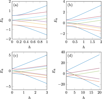
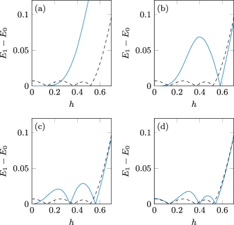
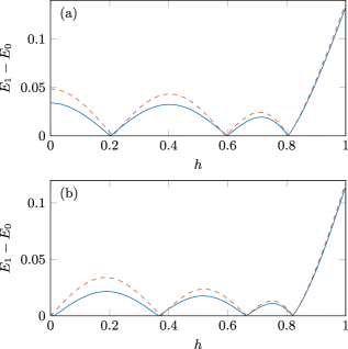
For a finite size chain, the twofold degeneracy of the TFI model at $0<h<h_{c}$ is lifted and there is a small non-vanishing energy splitting $\epsilon=E_{1}-E_{0}$ between the two lowest energy states, where the $E_{k}$ are the eigenenergies and $E_{k}\leq E_{k+1}~{}\forall k$. This splitting is exponentially suppressed with the system length, $\epsilon\sim\exp(-N/\xi)$ kitaev . These two quasi-degenerate states form a low energy sector separated from the higher energy states. The spectrum for $J_{z}=0$ and $N=3$ is shown in Fig. 1a. For $J_{z}>0$, the splitting $\epsilon$ has an oscillatory behaviour and vanishes for some values of $h$. For $N=3$, it vanishes once for $h>0$. See the spectrum for $J_{z}=0.5$ and $J_{z}=1$ in Figs 1b-c. As $J_{z}$ becomes large, there is no low energy sector separated from higher energy states any more. In the LFI limit, $J_{z}\to\infty$, the eigenstates have a well defined magnetisation in the $z$-direction and the energies are linear as a function of $h$, see Fig. 1d. In this limit, the level crossings are obvious. As the field is increased, the more polarised states become favoured, which leads to level crossings.

Figure 1: Exact diagonalisation spectrum as a function of $h$ for $N=3$ with $J_{z}=0$ (a), $J_{z}=0.5$ (b), $J_{z}=1$ (c) and $J_{z}=10$ (d).

Figure 2: Exact diagonalisation spectrum relative to the ground state energy, $E_{k}-E_{0}$, (a), two lowest energies $E_{0}$ and $E_{1}$ (c) and magnetisation $M=-{\partial}E_{0}/{\partial}h$ (e) as a function of $h$ for $N=6$ with $J_{z}=0$ (TFI limit). The plots in (b), (d) and (f) show the same for $J_{z}=0.75$.

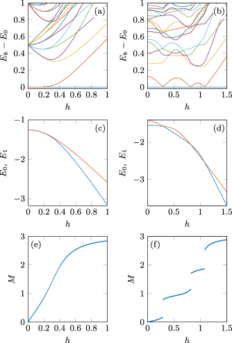
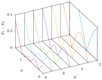
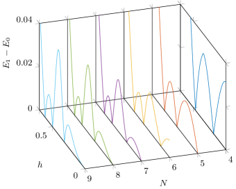
The plots in Fig. 1 are instructive for very small $N$ but become messy for larger chains. In Figs 2a-b, we show the spectrum relative to the ground state energy, i.e. $E_{k}-E_{0}$, of a chain of $N=6$ sites for $J_{z}=0$ and $J_{z}=0.75$. The energies $E_{0}$ and $E_{1}$ are plotted in Figs 2c-d for the same parameters. The structure of the spectrum is similar to the $N=3$ case, except that now $\epsilon$ vanishes at three points for $h>0$. In general, there are $N$ points of exact degeneracy where the splitting $\epsilon$ vanishes since the spectrum is symmetric under $h\to-h$. This is shown in Fig. 3 for $2\leq N\leq 8$. For $N$ even, there are $N/2$ level crossings for $h>0$, and for $N$ odd, there are $(N-1)/2$ level crossings for $h>0$ and one at $h=0$.

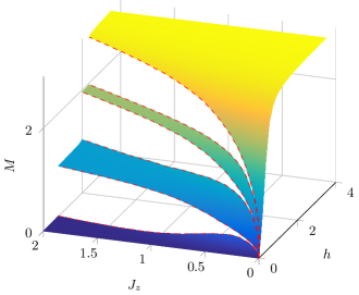
As shown in Figs 2e-f, the level crossings lead to jumps in the magnetisation $M(h)=-{\partial}E_{0}/{\partial}h$. The number of magnetisation jumps turns out to be independent of $J_{z}$ for $0<J_{z}<\infty$, as illustrated in Fig. 4. In the LFI limit, most of the jumps merge together at $h=J_{z}$, with an additional jump persisting for even $N$ at $h=J_{z}/2$ . In this large $J_{z}$ region, however, there is no quasi-degeneracy and the magnetisation jumps indicate level crossings but no oscillation in contrast to the small $J_{z}$ region. Since there are no level crossings in the TFI limit, one might expect the number of crossings to decrease as $J_{z}$ decreases. However, the exact diagonalisation results do not support this scenario, and hint to all level crossings appearing at the same time as soon as $J_{z}\neq 0$. This is a remarkable feature that we shall explain in the following.

A useful equivalent representation of the Hamiltonian in Eq. (1) in terms of spinless fermions is obtained by applying the Jordan-Wigner transformation used to solve exactly the TFI model pfeuty ,

$$\begin{cases}S_{i}^{x}=\frac{1}{2}(c_{i}^{\dagger}+c_{i})\exp\left({\mathrm{i}}\pi\sum_{j<i}c_{j}^{\dagger}c_{j}\right)\\ S_{i}^{y}=\frac{1}{2{\mathrm{i}}}(c_{i}^{\dagger}-c_{i})\exp\left({\mathrm{i}}\pi\sum_{j<i}c_{j}^{\dagger}c_{j}\right)\\ S_{i}^{z}=c_{i}^{\dagger}c_{i}-\frac{1}{2},\end{cases}$$ (2)

which yields

$$\begin{split}H&=\frac{1}{4}\sum_{i=1}^{N-1}(c_{i}^{\dagger}-c_{i})(c_{i+1}^{\dagger}+c_{i+1})-h\sum_{i=1}^{N}(c_{i}^{\dagger}c_{i}-\frac{1}{2})\\ &\quad+J_{z}\sum_{i=1}^{N-1}(c_{i}^{\dagger}c_{i}-\frac{1}{2})(c_{i+1}^{\dagger}c_{i+1}-\frac{1}{2})\end{split}$$ (3)

where the $c_{i},c_{i}^{\dagger}$ are fermionic annihilation and creation operators. This is the Hamiltonian of a spinless p-wave superconductor with nearest-neighbour density-density interaction. As for the simpler TFI model, the Hamiltonian is symmetric under a $\pi$-rotation of the spins around the $z$-axis, $S^{x}_{i}\to-S^{x}_{i}$ and $S^{y}_{i}\to-S^{y}_{i}$ in the spin language. This leads to two parity sectors given by the parity operator

$$P=e^{{\mathrm{i}}\pi\sum_{j=1}^{N}c_{j}^{\dagger}c_{j}}=(-2)^{N}S_{1}^{z}\cdots S_{N}^{z}.$$ (4)

In other words, the Hamiltonian does not mix states with even and odd number of up spins, or equivalently with even and odd number of fermions. The ground state parity changes at each point of exact degeneracy, and thus alternates as a function of the magnetic field for $J_{z}>0$. This can be understood qualitatively by looking at Fig. 2f. The magnetisation plateaus are roughly at $M=0,1,2,3$. Hence to jump from one plateau to the next, one spin has to flip, thus changing the sign of the parity $P$.

Figure 3: Exact diagonalisation energy splitting $\epsilon=E_{1}-E_{0}$ between the two lowest energy states as a function of $h$ for several $N$ and $J_{z}=0.75$. There are $N$ level crossings since the spectrum is symmetric under $h\to-h$.

Figure 4: Exact diagonalisation magnetisation $M$ as a function of $h$ and $J_{z}$ for $N=6$. The red dashed lines indicate the discontinuities.

II Perturbation theory

As a first attempt to understand if the $N$ level crossings develop immediately upon switching on $J_{z}$, we treat the $V=J_{z}\sum_{i=1}^{N-1}S^{z}_{i}S^{z}_{i+1}$ term as a perturbation to the exactly solvable transverse field Ising model. One may naively expect that degenerate perturbation theory is required since the TFI chain has a quasi-twofold degeneracy at low field. Fortunately, the two low-energy states live in different parity sectors pfeuty that are not mixed by the perturbation $V$. We can therefore apply the simple Rayleigh-Schrödinger perturbation theory in the range of parameters we are interested in, i.e. $J_{z}\lesssim 1$.

Figure 5: Energy splitting at zeroth (a), first (b), second (c) and third (d) order (blue solid lines) compared to the exact diagonalisation result (black dashed lines) for $N=6$ and $J_{z}=0.25$.

Figure 6: Energy splitting at third order in perturbation theory for several $N$ and $J_{z}=0.25$. Since the spectrum is symmetric under $h\to-h$, there are $N$ level crossings for $N\leq 7$ and $7$ level crossings for $N\geq 7$.

Writing $A_{i}=c_{i}^{\dagger}+c_{i}$ and $B_{i}=c_{i}^{\dagger}-c_{i}$, the perturbation can be rewritten as $V=({J_{z}}/{4})\sum_{i=1}^{N-1}B_{i}A_{i}B_{i+1}A_{i+1}$. The unperturbed eigenstates are $\ket{m}=\Upsilon^{\dagger}_{m}\ket{0}$ where $\ket{0}$ is the ground state and the $\Upsilon^{\dagger}_{m}$ are a product of the creation operators corresponding to the Bogoliubov fermions. The matrix elements are then

$$\begin{split}\braket{n}{V}{m}=\frac{J_{z}}{4}\sum_{i=1}^{N-1}\braket{0}{\Upsilon_{n}B_{i}A_{i}B_{i+1}A_{i+1}\Upsilon^{\dagger}_{m}}{0}\end{split}$$ (5)

which can be computed by applying Wick’s theorem, similarly to how correlation functions are found in lieb . We computed the effect of $V$ up to third order, with the basis of virtual states slightly truncated, namely by keeping states with at most three Bogoliubov fermions. Since the more fermions there are in a state, the larger its energy, we expect this approximation to be excellent.

As shown in Fig. 5, the number of crossings increases with the order of perturbation, and to third order in perturbation, the results for $N=6$ sites are in qualitative agreement with exact diagonalisations. From the way level crossings appear upon increasing the order of perturbation theory, one can expect to induce up to $2m+1$ level crossings if perturbation theory is pushed to order $m$, see Fig. 6. So these results suggest that the appearance of level crossings is a perturbative effect, and that, for a given size $N$, pushing perturbation theory to high enough order will indeed lead to $N$ level crossings for small $J_{z}$. However, in practice, it is impossible to push perturbation theory to very high order. Indeed, the results at order 3 are already very demanding. So, these pertubative results are encouraging, but they call for an alternative approach to actually prove that the number of level crossings is indeed equal to $N$, and that these level crossings appear as soon as $J_{z}$ is switched on.

III Fermionic mean-field approximation

Figure 7: Self-consistent mean-field parameters $\mu$ (blue solid lines and crosses), $t$ (red dotted lines and dots) and $\Delta$ (yellow dashed lines and squares) as a function of $h$ for $J_{z}=0.75$ and $N=6$ (a), as a function of $J_{z}$ for $h=0.4$ and $N=6$ (b) and as a function of $N$ for $h=0.4$ and $J_{z}=0.75$ (c).

In the fermionic representation, Eq. $\eqref{eqHfermions}$, there is a quartic term that cannot be treated exactly. Here, we approximate it by mean-field decoupling. In such an approximation, one assumes the system can be well approximated by a non-interacting system (quadratic in fermions) with self-consistently determined parameters. For generality, we decouple the quartic term in all three mean-field channels consistent with Wick’s theorem,

$$\begin{split}c^{\dagger}_{i}&c_{i}c^{\dagger}_{i+1}c_{i+1}\approx\\ &\braket{c^{\dagger}_{i}c_{i}}c^{\dagger}_{i+1}c_{i+1}+\braket{c^{\dagger}_{i+1}c_{i+1}}c^{\dagger}_{i}c_{i}-\braket{c^{\dagger}_{i}c_{i}}\braket{c^{\dagger}_{i+1}c_{i+1}}\\ -&\braket{c^{\dagger}_{i}c^{\dagger}_{i+1}}c_{i}c_{i+1}-\braket{c_{i}c_{i+1}}c^{\dagger}_{i}c^{\dagger}_{i+1}+\braket{c^{\dagger}_{i}c^{\dagger}_{i+1}}\braket{c_{i}c_{i+1}}\\ +&\braket{c^{\dagger}_{i}c_{i+1}}c_{i}c^{\dagger}_{i+1}+\braket{c_{i}c^{\dagger}_{i+1}}c^{\dagger}_{i}c_{i+1}-\braket{c^{\dagger}_{i}c_{i+1}}\braket{c_{i}c^{\dagger}_{i+1}}.\end{split}$$ (6)

Here, $\braket{.}$ denotes the ground state expectation value. The $3N-2$ self-consistent parameters $\braket{c^{\dagger}_{i}c_{i}}$, $\braket{c^{\dagger}_{i}c^{\dagger}_{i+1}}$ and $\braket{c^{\dagger}_{i}c_{i+1}}$ can be found straightforwardly by iteratively solving the quadratic mean-field Hamiltonian.

As it turns out, it is more instructive to consider only three self-consistent parameters. To do so, we solve the mean-field approximation of the translationally invariant Hamiltonian ($c_{N+1}=c_{1}$),

$$\begin{split}H^{\prime}&=\sum_{i=1}^{N}\left\{\frac{1}{4}(c_{i}^{\dagger}-c_{i})(c_{i+1}^{\dagger}+c_{i+1})-h(c_{i}^{\dagger}c_{i}-\frac{1}{2})\right.\\ &\left.+J_{z}(c_{i}^{\dagger}c_{i}-\frac{1}{2})(c_{i+1}^{\dagger}c_{i+1}-\frac{1}{2})\right\}\\ &\approx\sum_{i=1}^{N}\left\{-\mu c_{i}^{\dagger}c_{i}+(tc_{i+1}^{\dagger}c_{i}+{\rm h.c.})-(\Delta c_{i+1}^{\dagger}c^{\dagger}_{i}+{\rm h.c.})\right\}\\ &\quad+{\rm const},\end{split}$$ (7)

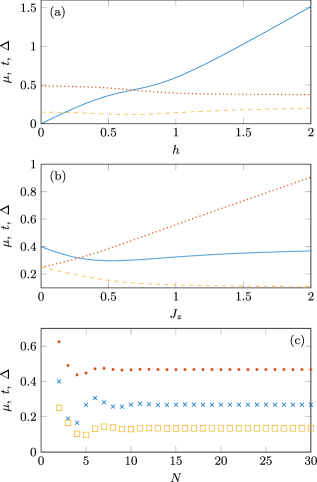
where $\mu=h+J_{z}(1-2\braket{c^{\dagger}_{i}c_{i}})$, $t=1/4-J_{z}\braket{c^{\dagger}_{i}c_{i+1}}$ and $\Delta=1/4-J_{z}\braket{c_{i}c_{i+1}}$ are determined self-consistently. These parameters are found to be real, and are shown in Fig. 7 as a function $h$, $J_{z}$ and $N$.

Using these self-consistent parameters, the Hamiltonian in Eq. (3) is then approximated by the following mean-field problem on an open chain:

$$\begin{split}H_{\rm MF}&=-\sum_{i=1}^{N}\mu\left(c^{\dagger}_{i}c_{i}-\frac{1}{2}\right)\\ &\quad+\sum_{i=1}^{N-1}\left[\left(tc^{\dagger}_{i+1}c_{i}+{\rm h.c.}\right)-\left(\Delta c^{\dagger}_{i+1}c^{\dagger}_{i}+{\rm h.c.}\right)\right],\end{split}$$ (8)

up to an irrelevant additive constant .

Figure 8: Critical fields, $h_{\rm crit}$, where the degeneracy is exact, as a function of $J_{z}$ in the self-consistent mean-field approximation (8) (blue crosses) compared to the exact diagonalisation result (red squares) for (a) $N=6$ and (b) $N=7$.

Figure 9: Energy splitting $\epsilon=E_{1}-E_{0}$ as a function of $h$ in the self-consistent mean-field approximation (8) (blue solid line) compared to the exact diagonalisation result (red dashed line) for $J_{z}=0.5$ and (a) $N=6$ and (b) $N=7$.

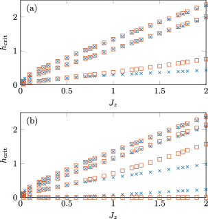
Since the self-consistent parameters are almost independent of the system size (see Fig. 7c), the boundaries are not very important and the bulk contribution is determinant. This partly justifies the approximation of playing with the boundary conditions to get the approximate model (8) with just three self-consistent parameters. This approximation is also justified by the great quantitative agreement with the exact diagonalisation results for the critical fields for $J_{z}\lesssim 0.8$ (see Fig. 8), and to a lesser extent for the energy splitting $\epsilon=E_{1}-E_{0}$ between the two lowest energy states, see Fig. 9.

For $N$ odd, the degeneracy at $h=0$ is protected by symmetry for any $J_{z}$ in the Hamiltonian (1). Indeed, under the transformation $S_{i}^{z}\to-S_{i}^{z}~{}\forall i$, the parity operator transforms as $P\to(-1)^{N}P$. Hence, for $N$ odd and $h=0$, the ground state has to be twofold degenerate. As can be seen in Fig. 8b, the critical field $h=0$ at low $J_{z}$ evolves to a non-zero value for large $J_{z}$, thus showing that this symmetry is broken by the mean-field approximation (8). The discrepancy is, however, small for $J_{z}\lesssim 0.8$ as can also be seen in Fig. 9b.

We observe from Fig. 7a that as a function of magnetic field, the parameters $t$ and $\Delta$ are almost constant, whereas $\mu$ is almost proportional to $h$. Thus, we can understand the physics of the level oscillations by forgetting about the self-consistency and considering $\mu$, $t$ and $\Delta$ as free parameters, i.e. by studying the open Kitaev chain kitaev , where the level crossings happen as $\mu$ is tuned. Compared to the TFI model for which $\Delta=t$, the main effect of $J_{z}>0$ is to make $0<\Delta<t$, which, as we shall see in the next section, is the condition to see level oscillations.

Such a mapping between the two lowest lying energy states of the interacting Kitaev chain and of the non-interacting Kitaev chain can be made rigorous for a special value of $h>0$, provided the boundary terms in equation (3) are slighty modified katsura . But this particular exact case misses out on level-crossing oscillations.

IV Level oscillations and Majorana fermions

We define $2N$ Majorana operators $\gamma^{\prime}_{i},~{}\gamma_{i}^{\prime\prime}$ as:

$$\begin{cases}\gamma^{\prime}_{i}=c_{i}+c^{\dagger}_{i}\\ \gamma^{\prime\prime}_{i}=-{\mathrm{i}}(c_{i}-c^{\dagger}_{i})\end{cases}$$ (9)

which satisfy ${\gamma^{\prime}}_{i}^{\dagger}=\gamma^{\prime}_{i}$, ${\gamma^{\prime\prime}}_{i}^{\dagger}=\gamma^{\prime\prime}_{i}$, $\{\gamma^{\prime}_{i},\gamma^{\prime\prime}_{j}\}=0$ and $\{\gamma^{\prime}_{i},\gamma^{\prime}_{j}\}=\{\gamma^{\prime\prime}_{i},\gamma^{\prime\prime}_{j}\}=2\delta_{ij}$. Since the $\mu,~{}t,~{}\Delta$ are real, the $H_{MF}$ of Eq. (8) reads

$$\begin{split}H_{\rm MF}=&\frac{{\mathrm{i}}}{2}\sum_{i=1}^{N-1}\left[-(t+\Delta)\gamma^{\prime\prime}_{i}\gamma^{\prime}_{i+1}+(t-\Delta)\gamma^{\prime}_{i}\gamma^{\prime\prime}_{i+1}\right]\\ &-\frac{{\mathrm{i}}\mu}{2}\sum_{i=1}^{N}\gamma^{\prime}_{i}\gamma^{\prime\prime}_{i}=\frac{{\mathrm{i}}}{2}\sum_{i,j=1}^{N}\gamma^{\prime}_{i}M_{ij}\gamma^{\prime\prime}_{j}.\end{split}$$ (10)

From the singular value decomposition of $M$, we write $M=U\Sigma V^{T}$, where $U$ and $V$ are orthogonal matrices and $\Sigma={\rm diag}(\epsilon_{1},\ldots,\epsilon_{N})$ with real $\epsilon_{i}$ and $|\epsilon_{i}|\leq|\epsilon_{i+1}|~{}\forall i$. Thus, the Hamiltonian reads

$$\begin{split}H_{\rm MF}&=\frac{{\mathrm{i}}}{2}\sum_{i,j,k=1}^{N}\gamma^{\prime}_{i}U_{ik}\epsilon_{k}V^{T}_{kj}\gamma^{\prime\prime}_{j}=\frac{{\mathrm{i}}}{2}\sum_{k=1}^{N}\epsilon_{k}\tilde{\gamma}^{\prime}_{k}\tilde{\gamma}^{\prime\prime}_{k}\\ &=\sum_{k}\epsilon_{k}(\eta^{\dagger}_{k}\eta_{k}-\frac{1}{2})\end{split}$$ (11)

where

$$\tilde{\gamma}^{\prime}_{k}=\sum_{i=1}^{N}\gamma^{\prime}_{i}U_{ik},\qquad\tilde{\gamma}^{\prime\prime}_{k}=\sum_{i=1}^{N}\gamma^{\prime\prime}_{i}V_{ik}$$ (12)

are the rotated Majorana operators, and the $\eta_{k}=\frac{1}{2}(\tilde{\gamma}^{\prime}_{k}+{\mathrm{i}}\tilde{\gamma}^{\prime\prime}_{k})$ are fermionic annihilation operators corresponding to the Bogoliubov quasiparticles.

As derived in Appendix, in general the Majorana operators, $\tilde{\gamma}^{\prime}_{k}$ and $\tilde{\gamma}^{\prime\prime}_{k}$, are of the form

$$\begin{split}\tilde{\gamma}^{\prime}_{k}=\sum_{j}(a_{+}x_{+}^{j}+b_{+}x_{+}^{N+1-j}+a_{-}x_{-}^{j}+b_{-}x_{-}^{N+1-j})\gamma^{\prime}_{j}\\ \tilde{\gamma}^{\prime\prime}_{k}=\sum_{j}(a_{+}x_{+}^{N+1-j}+b_{+}x_{+}^{j}+a_{-}x_{-}^{N+1-j}+b_{-}x_{-}^{j})\gamma^{\prime\prime}_{j}{}\end{split}$$ (13)

where the $x_{\pm}$, $a_{\pm}$ and $b_{\pm}$ are functions of the energy $\epsilon_{k}$ which is quantised in order to satisfy the boundary conditions. On can easily solve numerically the nonlinear equation for the $\epsilon_{k}$. Here, we will instead focus on a simple analytical approximation for $\tilde{\gamma}^{\prime}_{1},~{}\tilde{\gamma}^{\prime\prime}_{1}$ and $\epsilon_{1}$ which works well to discuss the level crossings, and is equivalent to the Ansatz given in kitaev .

From Eqs. (23) and (24), we see that for $\epsilon=0$, we have either $a_{\pm}=0$ or $b_{\pm}=0$. Without loss of generality, we can choose $b_{\pm}(\epsilon=0)=0$. Since we expect $\epsilon_{1}\ll 1$, we approximate

$$b_{\pm}(\epsilon_{1})\approx b_{\pm}(0)=0$$ (14)

and

$$x_{\pm}(\epsilon_{1})\approx x_{\pm}(0)=\frac{\mu\pm\sqrt{\mu^{2}-4t^{2}+4\Delta^{2}}}{2(t+\Delta)},$$ (15)

which yields

$$\begin{split}\tilde{\gamma}^{\prime}_{1}&\approx\sum_{j}(a_{+}x_{+}^{j}+a_{-}x_{-}^{j})\gamma^{\prime}_{j}\\ \tilde{\gamma}^{\prime\prime}_{1}&\approx\sum_{j}(a_{+}x_{+}^{N+1-j}+a_{-}x_{-}^{N+1-j})\gamma^{\prime\prime}_{j}\end{split}$$ (16)

with $\sum_{j}(a_{+}x_{+}^{j}+a_{-}x_{-}^{j})^{2}=1$. The boundary conditions (28) now read

$$a_{+}+a_{-} = 0$$ (17a)

$$a_{+}x_{+}^{N+1}+a_{-}x_{-}^{N+1} = 0$$ (17b)

and in general cannot be both satisfied unless $\epsilon_{1}=0$ exactly.

If $|x_{\pm}|<1$, $\tilde{\gamma}^{\prime}_{1}$ is localised on the left side of the chain with its amplitude $\sim e^{-j/\xi}$ as $j\gg 1$ with $\xi=-1/\ln(\max(|x_{+}|,|x_{-}|))$. Furthermore, $\tilde{\gamma}^{\prime\prime}_{1}$ is related to $\tilde{\gamma}^{\prime}_{1}$ by the reflection symmetry $j\to N+1-j$. Thus, in the thermodynamic limit, the boundary condition (17b) is irrelevant and $\epsilon_{1}\to 0$ as $N\to\infty$. Similarly, if $|x_{\pm}|>1$ the boundary condition (17a) becomes irrelevant in the thermodynamic limit. However, if $|x_{+}|>1$ and $|x_{-}|<1$, or $|x_{+}|<1$ and $|x_{-}|>1$, then $\tilde{\gamma}^{\prime}_{1}$, $\tilde{\gamma}^{\prime\prime}_{1}$ have significant weight on both sides of the chain and both boundary conditions (17a) and (17b) remain important in the thermodynamic limit. Hence, the approximation $\epsilon_{1}\approx 0$ is bad, indicating a gapped system. As discussed in kitaev , for $|\mu|<2|t|$ we have either $|x_{\pm}|<1$ or $|x_{\pm}|>1$ which yields $\epsilon_{1}=0$ in the thermodynamic limit. This is the topological phase with a twofold degenerate ground state. For a finite system, however, the boundary conditions (17a) and (17b) are in general not exactly satisfied and the system is only quasi-degenerate with a gap $\epsilon\sim e^{-N/\xi}$. For $|\mu|>2|t|$, either $|x_{+}|>1$ and $|x_{-}|<1$, or $|x_{+}|<1$ and $|x_{-}|>1$, and the system is gapped.

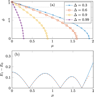
In the topological phase, $|\mu|<2|t|$, there are parameters for which the boundary conditions (17) can be exactly satisfied even for $N<\infty$ and thus $\epsilon_{1}=0$ exactly. In such a case, there is an exact zero mode even for a finite chain. This was previously discussed in Ref. kao , as well as in hedge where a more general method that applies to disordered systems is described. If $x_{\pm}\in\mathbb{R}$, it is never possible to satisfy the boundary conditions (17) and therefore the quasi-gap is always finite, $\epsilon_{1}\neq 0$. However, if $x_{+}=re^{{\mathrm{i}}\phi}\not\in\mathbb{R}$, Eq. (15) yields $x_{-}=x_{+}^{*}$ and $(x_{+}^{N+1}-x_{-}^{N+1})\propto r^{N+1}\sin[(N+1)\phi]$. Thus it may happen for specific parameters that $\epsilon_{1}=0$ exactly. This degeneracy indicates a level crossing. The phase $\phi$, defined for $|\mu|<\mu_{c}=2\sqrt{t^{2}-\Delta^{2}}$, is given by

$$\tan{\phi}=\sqrt{(\mu_{c}/\mu)^{2}-1}.$$ (18)

It thus goes continuously from $\phi(\mu=0^{+})=\pi/2$ to $\phi(\mu\to\mu_{c})\to 0$. Hence, there are critical chemical potentials, $0\leq\mu_{\lceil N/2\rceil}<\ldots<\mu_{m}<\ldots<\mu_{1}<\mu_{c}$, such that $\phi(\mu=\mu_{m})=\frac{\pi m}{N+1}$ (see Fig. 10a). For these critical $\mu_{m}$, the system is exactly degenerate, i.e. $\epsilon_{1}=0$. In the TFI limit, we have $\Delta=t$ and $\mu_{c}=0$, thus there are no level crossings.

Figure 10: (a) Phase $\phi(\mu)$ of $x_{+}=re^{{\mathrm{i}}\phi}$ within the approximation (15) for several $\Delta$ with $t=1$ and $N=6$. The horizontal black dotted lines indicate the values $\phi=\frac{\pi m}{N+1}$. (b) Splitting $E_{1}-E_{0}=|\epsilon_{1}|$ in the Kitaev chain calculated exactly solving numerically the full self-consistent equations described in Appendix (blue solid line) and with the analytical approximate result in Eq. (19) (red dashed line) for $N=6$, $t=1$ and $\Delta=0.3$.

For $|\mu|<2|t|$, writing $x_{+}=re^{{\mathrm{i}}\phi}$ with $r>0$, we have

$$\begin{split}\epsilon_{1}&=\Sigma_{11}=(U^{T}MV)_{11}\\ &\approx 4(t+\Delta)a_{+}^{2}r^{N+2}\sin(\phi)\sin[(N+1)\phi],\end{split}$$ (19)

where we used the approximations (15), (16) and the boundary condition (17a) [respectively (17b)] when $t\Delta>0$ (respectively $t\Delta<0$), since in this case $|x_{\pm}|<1$ (respectively $|x_{\pm}|>1$). Note that $\phi(-\mu)=\phi(\mu)-\pi$, and thus $\epsilon_{1}$ is an odd function of $\mu$ for odd $N$ and an even function of $\mu$ for even $N$. Since $\epsilon_{1}$ changes sign whenever $\sin((N+1)\phi)=0$, the degeneracy points indicate level crossings. This approximate description works extremely well, as shown in Fig. 10b for $\Delta=0.3t$. Because $\phi$ takes all the values in $]0,\pi/2]$ for $0<\mu<\mu_{c}$, and in $]-\pi,-\pi/2]$ for $-\mu_{c}<\mu<0$, there are either exactly $N$ level crossings as a function of $\mu$ if $0<\mu_{c}\in\mathbb{R}$, i.e. if $|\Delta|<|t|$, and no zero level crossing otherwise. At the points of exact degeneracy, $b_{\pm}(\epsilon=0)=0$, the zero-mode Majorana fermions are localised on opposite sides of the chain. When the degeneracy is not exact, however, $b_{\pm}(\epsilon\neq 0)\neq 0$ and the zero-mode Majorana fermions mix together to form Majoranas localised mostly on one side but also a little bit on the opposite side.

In the XY model in an out-of-plane magnetic field, which is equivalent to the non-interacting Kitaev chain lieb , these level crossings lead to an oscillatory behaviour of the spin correlation functions barouch . In the context of p-wave superconductors, the level oscillations described above also arise in more realistic models and are considered one of the hallmarks of the presence of topological Majorana fermions sarma ; loss . Although it is still debated whether Majorana fermions have already been observed, strong experimental evidence for the level oscillations was reported in markus .

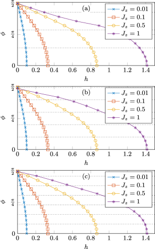
Coming back to the mean-field Hamiltonian of Eq. (6), we can get the phase $\phi$ within the approximation (15), i.e. the phase of $x_{+}(\epsilon=0)$, as a function of the physical parameters $h,~{}J_{z}$ since we know how the self-consistent parameters $\mu,~{}t,~{}\Delta$ depend on them. We plot in Fig. 11 the phase $\phi$ as a function of $h$ for several $J_{z}$ which yields a good qualitative understanding of the sudden appearance of $N$ level crossings as soon as $J_{z}>0$. As previously discussed, the self-consistent parameters are almost independent of $N$ and therefore the curves $\phi(h)$ are almost independent of $N$ as well. The main effect of $N$ is to change the condition $\phi(\mu=\mu_{m})=\frac{\pi m}{N+1}$ for the boundary condition in Eq. (17b) to be satisfied and thus for the system to be exactly degenerate.

Figure 11: Phase $\phi(h)$ of $x_{+}(\epsilon=0)$ based on the self-consistent parameters $\mu,~{}t,~{}\Delta$ of the mean-field decoupling for several $J_{z}$ and (a) $N=6$, (b) $N=9$, (c) $N=12$. The horizontal black dotted lines indicate the values $\phi=\frac{\pi m}{N+1}$.

V Summary

The main result of this paper is that the level crossings between the two lowest energy eigenstates of the XY chain in an in-plane magnetic field are more generally a fundamental feature of the transverse field Ising chain with an antiferromagnetic longitudinal coupling howsoever small. These points of level crossings (twofold degeneracy) correspond to having Majorana edge modes in a Kitaev chain onto which the problem can be approximately mapped. The level crossings of the XY chains have been observed experimentally in toskovic by scanning tunneling microscopy on Cobalt atoms evaporated onto a Cu₂N/Cu(100) substrate. By varying the adsorbed atoms and the substrate, it should be possible to vary the easy-plane and easy-axis anisotropies, and thus to explore the exact degeneracy points for various values of the longitudinal coupling. The possibility to probe the two-fold degeneracy of this family of spin chains is important in view of their potential use for universal quantum computation loss2 . Besides, one could also realise the spinless fermionic Hamiltonian (3) in an array of Josephson junctions as described in hassler . The advantage of this realisation is that it allows a great flexibility to tune all the parameters of the model. We hope that the results of the present paper will stimulate experimental investigations along these lines.

*

Appendix A Majorana solutions of the Kitaev chain

To solve the Kitaev chain (8), we need to find the singular value decomposition of

$$M=\begin{pmatrix}-\mu&\tau_{-}&0&\cdots\\ \tau_{+}&-\mu&\tau_{-}&0&\cdots\\ 0&\tau_{+}&-\mu&\tau_{-}&0&\cdots\\ &&\ddots&\ddots&\ddots&\\ &\cdots&0&\tau_{+}&-\mu&\tau_{-}\\ &&\cdots&0&\tau_{+}&-\mu\end{pmatrix}$$ (20)

with $\tau_{\pm}=t\pm\Delta$, i.e. find orthogonal matrices $U$, $V$ and a real diagonal matrix $\Sigma$ such that $M=U\Sigma V^{T}$. Writing $\vec{u}_{k}$ and $\vec{v}_{k}$ the $k^{\rm th}$ columns of $U$ and $V$ respectively, they satisfy

$$\begin{cases}M\vec{v}_{k}&=\epsilon_{k}\vec{u}_{k}\\ \vec{u}_{k}^{T}M&=\epsilon_{k}\vec{v}_{k}^{T}.\end{cases}$$ (21)

Let’s find two unit-norm column vectors $\vec{u},~{}\vec{v}$ and $\epsilon$ such that $M\vec{v}=\epsilon\vec{u}$ and $\vec{u}^{T}M=\epsilon\vec{v}^{T}$. First we forget about the normalisation and boundary conditions and focus on the secular equation. Setting the components of $\vec{u},~{}\vec{v}$ as $u_{j}=ax^{j}$ and $v_{j}=bx^{j}$, we have

$$\begin{split}M\vec{v}&=\frac{b}{a}\frac{\tau_{+}-\mu x+\tau_{-}x^{2}}{x}\vec{u}+{\rm b.t.}\\ \vec{u}^{T}M&=\frac{a}{b}\frac{\tau_{-}-\mu x+\tau_{+}x^{2}}{x}\vec{v}^{T}+{\rm b.t.}\end{split}$$ (22)

where b.t. stands for boundary terms. Hence, $u$ and $v$ satisfy the secular equation provided

$$\frac{b}{a}=\sqrt{\frac{\tau_{-}-\mu x+\tau_{+}x^{2}}{\tau_{+}-\mu x+\tau_{-}x^{2}}}$$ (23)

and

$$\epsilon=\frac{1}{x}\sqrt{(\tau_{-}-\mu x+\tau_{+}x^{2})(\tau_{+}-\mu x+\tau_{-}x^{2})}.$$ (24)

Because of the reflection symmetry $j\to N+1-j$, if $x$ is a solution of equation (24) for some $\epsilon$, then $1/x$ is also a solution. Assuming $\epsilon$ known, the solutions are $x_{\pm}$, $1/x_{\pm}$ and satisfy

$$\begin{split}0&=\epsilon^{2}x^{2}-(\tau_{-}-\mu x+\tau_{+}x^{2})(\tau_{+}-\mu x+\tau_{-}x^{2})\\ &\propto(x-x_{+})(x-1/x_{+})(x-x_{-})(x-1/x_{-})\end{split}$$ (25)

which by identification yields, writing $\rho_{\pm}=x_{\pm}+1/x_{\pm}$,

$$\begin{split}x_{\pm}&=\frac{1}{2}\left(\rho_{\pm}+\sqrt{\rho_{\pm}^{2}-4}\right),\\ \rho_{\pm}&=\frac{\mu t\pm\sqrt{(t^{2}-\Delta^{2})\epsilon^{2}+\Delta^{2}(\mu^{2}-4t^{2}+4\Delta^{2})}}{t^{2}-\Delta^{2}}.\end{split}$$ (26)

Taking into account the reflection symmetry, the general form of the components of $\vec{u},~{}\vec{v}$ is thus

$$\begin{split}u_{j}=a_{+}x_{+}^{j}+b_{+}x_{+}^{N+1-j}+a_{-}x_{-}^{j}+b_{-}x_{-}^{N+1-j}\\ v_{j}=a_{+}x_{+}^{N+1-j}+b_{+}x_{+}^{j}+a_{-}x_{-}^{N+1-j}+b_{-}x_{-}^{j}\end{split}$$ (27)

with the ratios $b_{+}/a_{+}$ and $b_{-}/a_{-}$ given by equation (23) with $x=x_{+}$ and $x=x_{-}$ respectively.

Furthermore, we have the boundary conditions

$$\begin{split}a_{+}+b_{+}x_{+}^{N+1}+a_{-}+b_{-}x_{-}^{N+1}&=0\\ a_{+}x_{+}^{N+1}+b_{+}+a_{-}x_{-}^{N+1}+b_{-}&=0\end{split}$$ (28)

which set the ratio $a_{-}/a_{+}$ and give the quantisation condition on the energies $\epsilon_{k}$. The last degree of freedom, say $a_{+}$, is then set by normalising $\vec{u}$ (from equation (27), $\|\vec{u}\|=\|\vec{v}\|$).

Note that for the special cases $t=\Delta$ and $\mu=0$, we have $\tilde{\gamma}^{\prime}_{1}=\gamma^{\prime}_{1}$ and $\tilde{\gamma}^{\prime\prime}_{1}=\gamma^{\prime\prime}_{N}$ with $\epsilon_{1}=0$. We have a similar result for $t=-\Delta$ and $\mu=0$. For these two cases, the general formalism described above does not apply since it yields $x_{\pm}=0,\pm\infty$.

References

- (1) M. Z. Hasan and C. L. Kane, Rev. Mod. Phys. 82, 3045 (2010).
- (2) X.-L. Qi and S.-C. Zhang, Rev. Mod. Phys. 83, 1057 (2011).
- (3) F. D. M. Haldane, Phys. Lett. A 93, 464 (1983).
- (4) T. Kennedy, J. Phys. Cond. Mat. 2, 5737 (1990).
- (5) F. Tedoldi, R. Santachiara, and M. Horvatić, Phys. Rev. Lett. 83, 412 (1999).
- (6) A. Y. Kitaev. Phys.-Usp. 44 131 (2001).
- (7) V. Mourik, K. Zuo, S. M. Frolov, S. R. Plissard, E. P. A. M. Bakkers, and L. P. Kouwenhoven, Science 336, 1003 (2012).
- (8) S. Nadj-Perge, I. K. Drozdov, J. Li, H. Chen, S. Jeon, J. Seo, A. H. MacDonald, B. A. Bernevig, and A. Yazdani, Science 346, 602 (2014).
- (9) S. Das Sarma, J. D. Sau, and T. D. Stanescu, Phys. Rev. B 86, 220506(R) (2012).
- (10) R. Toskovic, R. van den Berg, A. Spinelli, I. S. Eliens, B. van den Toorn, B. Bryant, J.-S. Caux, and A. F. Otte, Nat. Phys. 12, 656 (2016).
- (11) D. V. Dmitriev, V. Y. Krivnov, A. A. Ovchinnikov, and A. Langari, J. Exp. Theor. Phys. 95, 538 (2002).
- (12) F. Mila, Nat. Phys. 12, 633 (2016).
- (13) P. Pfeuty, Ann. Phys. 57, 79 (1970).
- (14) S. Suzuki, J.-i. Inoue, and B. K. Chakrabarti, Quantum Ising Phases and Transitions in Transverse Ising Models (Springer, Lecture Notes in Physics, Vol. 862 (2013)).
- (15) S. Jalal and B. Kumar, Phys. Rev. B 90, 184416 (2014).
- (16) P. Ruján, Phys. Rev. B 24, 6620 (1981).
- (17) F. Hassler and D. Schuricht, New J. Phys. 14, 125018 (2012).
- (18) E. Lieb, T. Schultz, and D. Mattis, Ann. Phys. 16, 407 (1961).
- (19) H. Katsura, D. Schuricht, and M. Takahashi, Phys. Rev. B 92, 115137 (2015).
- (20) H.-C. Kao, Phys. Rev. B 90, 245435 (2014).
- (21) S. S. Hegde, and S. Vishveshwara, Phys. Rev. B 94, 115166 (2016).
- (22) E. Barouch and B. M . McCoy, Phys. Rev. A3, 786 (1971).
- (23) D. Rainis, L. Trifunovic, J. Klinovaja, and D. Loss, Phys. Rev. B 87, 024515 (2013).
- (24) S. M. Albrecht, A. P. Higginbotham, M. Madsen, F. Kuemmeth, T. S. Jespersen, J. Nygård, P. Krogstrup, and C. M. Marcus, Nature 531, 206 (2016).
- (25) Y. Tserkovnyak and D. Loss, Phys. Rev. A 84, 032333 (2011).