Modelling Competitive Sports:
Bradley-Terry-Élő Models
for Supervised and On-Line Learning
of Paired Competition Outcomes

Abstract

Prediction and modelling of competitive sports outcomes has received much recent attention, especially from the Bayesian statistics and machine learning communities. In the real world setting of outcome prediction, the seminal Élő update still remains, after more than 50 years, a valuable baseline which is difficult to improve upon, though in its original form it is a heuristic and not a proper statistical “model”. Mathematically, the Élő rating system is very closely related to the Bradley-Terry models, which are usually used in an explanatory fashion rather than in a predictive supervised or on-line learning setting.

Exploiting this close link between these two model classes and some newly observed similarities, we propose a new supervised learning framework with close similarities to logistic regression, low-rank matrix completion and neural networks. Building on it, we formulate a class of structured log-odds models, unifying the desirable properties found in the above: supervised probabilistic prediction of scores and wins/draws/losses, batch/epoch and on-line learning, as well as the possibility to incorporate features in the prediction, without having to sacrifice simplicity, parsimony of the Bradley-Terry models, or computational efficiency of Élő’s original approach.

We validate the structured log-odds modelling approach in synthetic experiments and English Premier League outcomes, where the added expressivity yields the best predictions reported in the state-of-art, close to the quality of contemporary betting odds.

1.  Introduction

1.1.  Modelling and predicting competitive sports

Competitive sports refers to any sport that involves two teams or individuals competing against each other to achieve higher scores. Competitive team sports includes some of the most popular and most watched games such as football, basketball and rugby. Such sports are played both in domestic professional leagues such as the National Basketball Association, and international competitions such as the FIFA World Cup. For football alone, there are over one hundred fully professional leagues in 71 countries globally. It is estimated that the Premier League, the top football league in the United Kingdom, attracted a (cumulative) television audience of 4.7 billion viewers in the last season [47].

The outcome of a match is determined by a large number of factors. Just to name a few, they might involve the competitive strength of each individual player in both teams, the smoothness of collaboration between players, and the team’s strategy of playing. Moreover, the composition of any team changes over the years, for example because players leave or join the team. The team composition may also change within the tournament season or even during a match because of injuries or penalties.

Understanding these factors is, by the prediction-validation nature of the scientific method, closely linked to predicting the outcome of a pairing. By Occam’s razor, the factors which empirically help in prediction are exactly those that one may hypothesize to be relevant for the outcome.

Since keeping track of all relevant factors is unrealistic, of course one cannot expect a certain prediction of a competitive sports outcome. Moreover, it is also unreasonable to believe that all factors can be measured or controlled, hence it is reasonable to assume that unpredictable, or non-deterministic statistical “noise” is involved in the process of generating the outcome (or subsume the unknowns as such noise). A good prediction will, hence, not exactly predict the outcome, but will anticipate the “correct” odds more precisely. The extent to which the outcomes are predictable may hence be considered as a surrogate quantifier of how much the outcome of a match is influenced by “skill” (as surrogated by determinism/prediction), or by “chance” (as surrogated by the noise/unknown factors).

Phenomena which can not be specified deterministically are in fact very common in nature. Statistics and probability theory provide ways to make inference under randomness. Therefore, modelling and predicting the results of competitive team sports naturally falls into the area of statistics and machine learning. Moreover, any interpretable predictive model yields a possible explanation of what constitutes factors influencing the outcome.

1.2.  History of competitive sports modelling

Research of modeling competitive sports has a long history. In its early days, research was often closely related to sports betting or player/team ranking [22, 26]. The two most influential approaches are due to Bradley and Terry [3] and Élő [15]. The Bradley-Terry and Élő models allow estimation of player rating; the Élő system additionally contains algorithmic heuristics to easily update a player’s rank, which have been in use for official chess rankings since the 1960s. The Élő system is also designed to predict the odds of a player winning or losing to the opponent. In contemporary practice, Bradley-Terry and Élő type models are broadly used in modelling of sports outcomes and ranking of players, and it has been noted that they are very close mathematically.

In more recent days, relatively diverse modelling approaches originating from the Bayesian statistical framework  [37, 13, 20], and also some inspired by machine learning principles [36, 23, 43] have been applied for modelling competitive sports. These models are more expressive and remove some of the Bradley-Terry and Élő models’ limitations, though usually at the price of interpretability, computational efficiency, or both.

A more extensive literature overview on existing approaches will be given later in Section 3, as literature spans multiple communities and, in our opinion, a prior exposition of the technical setting and simultaneous straightening of thoughts benefits the understanding and allows us to give proper credit and context for the widely different ideas employed in competitive sports modelling.

1.3.  Aim of competitive sports modelling

In literature, the study of competitive team sports may be seen to lie between two primary goals. The first goal is to design models that make good predictions for future match outcome. The second goal is to understand the key factors that influence the match outcome, mostly through retrospective analysis [45, 50]. As explained above, these two aspects are intrinsically connected, and in our view they are the two facets of a single problem: on one hand, proposed influential factors are only scientifically valid if confirmed by falsifiable experiments such as predictions on future matches. If the predictive performance does not increase when information about such factors enters the model, one should conclude by Occam’s razor that these factors are actually irrelevant. On the other hand, it is plausible to assume that predictions are improved by making use of relevant factors (also known as “features”) become available, for example because they are capable of explaining unmodelled random effects (noise). In light of this, the main problem considered in this work is the (validable and falsifiable) prediction problem, which in machine learning terminology is also known as the supervised learning task.

1.4.  Main questions and challenges in competitive sports outcomes prediction

Given the above discussion, the major challenges may be stated as follows:

On the methodological side, what are suitable models for competitive sports outcomes? Current models are not at the same time interpretable, easily computable, allow to use feature information on the teams/players, and allow to predict scores or ternary outcomes. It is an open question how to achieve this in the best way, and this manuscript attempts to highlight a possible path.

The main technical difficulty lies in the fact that off-shelf methods do not apply due to the structured nature of the data: unlike in individual sports such as running and swimming where the outcome depends only on the given team, and where the prediction task may be dealt with classical statistics and machine learning technology (see [2] for a discussion of this in the context of running), in competitive team sports the outcome may be determined by potentially complex interactions between two opposing teams. In particular, the performance of any team is not measured directly using a simple metric, but only in relation to the opposing team’s performance.

On the side of domain applications, which in this manuscript is premier league football, it is of great interest to determine the relevant factors determining the outcome, the best way to predict, and which ranking systems are fair and appropriate.

All these questions are related to predictive modelling, as well as the availability of suitable amounts of quality data. Unfortunately, the scarcity of features available in systematic presentation places a hurdle to academic research in competitive team sports, especially when it comes to assessing important factors such as team member characteristics, or strategic considerations during the match.

Moreover, closely linked is also the question to which extent the outcomes are determined by “chance” as opposed to “skill”. Since if on one hypothetical extreme, results would prove to be completely unpredictable, there would be no empirical evidence to distinguish the matches from a game of chance such as flipping a coin. On the other hand, importance of a measurement for predicting would strongly suggest its importance for winning (or losing), though without an experiment not necessarily a causative link.

We attempt to address these questions in the case of premier league football within the confines of readily available data.

1.5.  Main contributions

Our main contributions in this manuscript are the following:

• We give what we believe to be the first comprehensive literature review of state-of-art competitive sports modelling that comprises the multiple communities (Bradley-Terry models, Élő type models, Bayesian models, machine learning) in which research so far has been conducted mostly separately.

• We present a unified Bradley-Terry-Élő model which combines the statistical rigour of the Bradley-Terry models with fitting and update strategies similar to that found in the Élő system. Mathematically only a small step, this joint view is essential in a predictive/supervised setting as it allows efficient training and application in an on-line learning situation. Practically, this step solves some problems of the Élő system (including ranking initialization and choice of K-factor), and establishes close relations to logistic regression, low-rank matrix completion, and neural networks.

• This unified view on Bradley-Terry-Élő allows us to introduce classes of joint extensions, the structured log-odds models, which unites desirable properties of the extensions found in the disjoint communities: probabilistic prediction of scores and wins/draws/losses, batch/epoch and on-line learning, as well as the possibility to incorporate features in the prediction, without having to sacrifice structural parsimony of the Bradley-Terry models, or simplicity and computational efficiency of Élő’s original approach.

• We validate the practical usefulness of the structured log-odds models in synthetic experiments and in answering domain questions on English Premier League data, most prominently on the importance of features, fairness of the ranking, as well as on the “chance”-“skill” divide.

1.6.  Manuscript structure

Section 2 gives an overview of the mathematical setting in competitive sports prediction. Building on the technical context, Section 3 presents a more extensive review of the literature related to the prediction problem of competitive sports, and introduces a joint view on Bradley-Terry and Élő type models. Section 4 introduces the structured log-odds models, which are validated in empirical experiments in Section 5. Our results and possible future directions for research are discussed in section 6.

Authors’ contributions

This manuscript is based on ZQ’s MSc thesis, submitted September 2016 at University College London, written under supervision of FK. FK provided the ideas of re-interpretation and possible extensions of the Élő model. Literature overview is jointly due to ZQ an FQ, and in parts follows some very helpful pointers by I. Kosmidis (see below). Novel technical ideas in Sections 4.2 to 4.4, and experiments (set-up and implementation) are mostly due to ZQ.

The present manuscript is a substantial re-working of the thesis manuscript, jointly done by FK and ZQ.

Acknowledgements

We are thankful to Ioannis Kosmidis for comments on an earlier form of the manuscript, for pointing out some earlier occurrences of ideas presented in it but not given proper credit, as well as relevant literature in the “Bradley-Terry” branch.

2.  The Mathematical-Statistical Setting

This section formulates the prediction task in competitive sports and fixes notation, considering as an instance of supervised learning with several non-standard structural aspects being of relevance.

2.1.  Supervised prediction of competitive outcomes

We introduce the mathematical setting for outcome prediction in competitive team sports. As outlined in the introductory Section 1.1, three crucial features need to be taken into account in this setting:

• The outcome of a pairing cannot be exactly predicted prior to the game, even with perfect knowledge of all determinates. Hence it is preferable to predict a probabilistic estimate for all possible match outcomes (win/draw/loss) rather than deterministically choosing one of them.

• In a pairing, two teams play against each other, one as a home team and the other as the away or guest team. Not all pairs may play against each other, while others may play multiple times. As a mathematically prototypical (though inaccurate) sub-case one may consider all pairs playing exactly once, which gives the observations an implicit matrix structure (row = home team, column = away team). Outcome labels and features crucially depend on the teams constituting the pairing.

• Pairings take place over time, and the expected outcomes are plausibly expected to change with (possibly hidden) characteristics of the teams. Hence we will model the temporal dependence explicitly to be able to take it into account when building and checking predictive strategies.

2.1.1.  The Generative Model.

Following the above discussion, we will fix a generative model as follows: as in the standard supervised learning setting, we will consider a generative joint random variable $(X,Y)$ taking values in $\mathcal{X}\times\mathcal{Y}$, where $\mathcal{X}$ is the set of features (or covariates, independent variables) for each pairing, while $\mathcal{Y}$ is the set of labels (or outcome variables, dependent variables).

In our setting, we will consider only the cases $\mathcal{Y}=\{\text{win},\,\text{lose}\}$ and $\mathcal{Y}=\{\text{win},\,\text{lose},\,\text{draw}\}$, in which case an observation from $\mathcal{Y}$ is a so-called match outcome, as well as the case $\mathcal{Y}=\mathbb{N}^{2}$, in which case an observation is a so-called final score (in which case, by convention, the first component of $\mathcal{Y}$ is of the home team), or the case of score differences where $\mathcal{Y}=\mathbb{N}$ (in which case, by convention, a positive number is in favour of the home team). From the official rule set of a game (such as football), the match outcome is uniquely determined by a score or score difference. As all the above sets $\mathcal{Y}$ are discrete, predicting $\mathcal{Y}$ will amount to supervised classification (the score difference problem may be phrased as a regression problem, but we will abstain from doing so for technical reasons that become apparent later).

The random variable $X$ and its domain $\mathcal{X}$ shall include information on the teams playing, as well as on the time of the match.

We will suppose there is a set $\mathcal{I}$ of teams, and for $i,j\in\mathcal{I}$ we will denote by $(X_{ij},Y_{ij})$ the random variable $(X,Y)$ conditioned on the knowledge that $i$ is the home team, and $j$ is the away team. Note that information in $X_{ij}$ can include any knowledge on either single team $i$ or $j$, but also information corresponding uniquely to the pairing $(i,j)$.

We will assume that there are $Q:=\#\mathcal{I}$ teams, which means that the $X_{ij}$ and $Y_{ij}$ may be arranged in $(Q\times Q)$ matrices each.

Further there will be a set $\mathcal{T}$ of time points at which matches are observed. For $t\in\mathcal{T}$ we will denote by $(X(t),Y(t))$ or $(X_{ij}(t),Y_{ij}(t))$ an additional conditioning that the outcome is observed at time point $t$.

Note that the indexing $X_{ij}(t)$ and $Y_{ij}(t)$ formally amounts to a double conditioning and could be written as $X|I=i,J=j,T=t$ and $Y|I=i,J=j,T=t$, where $I,J,T$ are random variables denoting the home team, the away team, and the time of the pairing. Though we do believe that the index/bracket notation is easier to carry through and to follow (including an explicit mirroring of the the “matrix structure”) than the conditional or “graphical models” type notation, which is our main reason for adopting the former and not the latter.

2.1.2.  The Observation Model.

By construction, the generative random variable $(X,Y)$ contains all information on having any pairing playing at any time, However, observations in practice will concern two teams playing at a certain time, hence observations in practice will only include independent samples of $(X_{ij}(t),Y_{ij}(t))$ for some $i,j\in\mathcal{I},t\in\mathcal{T}$, and never full observations of $(X,Y)$ which can be interpreted as a latent variable.

Note that the observations can be, in-principle, correlated (or unconditionally dependent) if the pairing $(i,j)$ or the time $t$ is not made explicit (by conditioning which is implicit in the indices $i,j,t$).

An important aspect of our observation model will be that whenever a value of $X_{ij}(t)$ or $Y_{ij}(t)$ is observed, it will always come together with the information of the playing teams $(i,j)\in\mathcal{I}^{2}$ and the time $t\in\mathcal{T}$ at which it was observed. This fact will be implicitly made use of in description of algorithms and validation methodology. (formally this could be achieved by explicitly exhibiting/adding $\mathcal{I}\times\mathcal{I}\times\mathcal{T}$ as a Cartesian factor of the sampling domains $\mathcal{X}$ or $\mathcal{Y}$ which we will not do for reasons of clarity and readability)

Two independent batches of data will be observed in the exposition. We will consider:

$$\mbox{a training set}\;\mathcal{D} :=\{(X^{(1)}_{i_{1}j_{1}}(t_{1}),Y^{(1)}_{i_{1}j_{1}}(t_{1})),\dots,(X^{(N)}_{i_{N}j_{N}}(t_{N}),Y^{(N)}_{i_{N}j_{N}}(t_{N}))\}$$

$$\mbox{a test set}\;\mathcal{T} :=\{(X^{(1*)}_{i^{*}_{1}j^{*}_{1}}(t^{*}_{1}),Y^{(1*)}_{i^{*}_{1}j^{*}_{1}}(t^{*}_{1})),\dots,(X^{(M*)}_{i^{*}_{M}j^{*}_{M}}(t^{*}_{M}),Y^{(M*)}_{i^{*}_{M}j^{*}_{M}}(t^{*}_{M}))\}$$

where $(X^{(i)},Y^{(i)})$ and $(X^{(i*)},Y^{(i*)})$ are i.i.d. samples from $(X,Y)$.

Note that unfortunately (from a notational perspective), one cannot omit the superscripts $\kappa$ as in $X^{(\kappa)}$ when defining the samples, since the figurative “dies” should be cast anew for each pairing taking place. In particular, if all games would consist of a single pair of teams playing where the results are independent of time, they would all be the same (and not only identically distributed) without the super-index, i.e., without distinguishing different games as different samples from $(X,Y)$.

2.1.3.  The Learning Task.

As set out in the beginning, the main task we will be concerned with is predicting future outcomes given past outcomes and features, observed from the process above. In this work, the features will be assumed to change over time slowly. It is not our primary goal to identify the hidden features in $(X,Y)$, as they are never observed and hence not accessible as ground truth which can validate our models. However, these will be of secondary interest and considered empirically validated by a well-predicting model.

More precisely, we will describe methodology for learning and validating predictive models of the type

$$f:\mathcal{X}\times\mathcal{I}\times\mathcal{I}\times\mathcal{T}\rightarrow\operatorname{Distr}(\mathcal{Y}),$$

where $\operatorname{Distr}(\mathcal{Y})$ is the set of (discrete probability) distributions on $\mathcal{Y}$. That is, given a pairing $(i,j)$ and a time point $t$ at which the teams $i$ and $j$ play, and information of type $x=X_{ij}(t)$, make a probabilistic prediction $f(x,i,j,t)$ of the outcome.

Most algorithms we discuss will not use added information in $\mathcal{X}$, hence will be of type $f:\mathcal{I}\times\mathcal{I}\times\mathcal{T}\rightarrow\operatorname{Distr}(\mathcal{Y})$. Some will disregard the time in $\mathcal{T}$. Indeed, the latter algorithms are to be considered scientific baselines above which any algorithm using information in $\mathcal{X}$ and/or $\mathcal{T}$ has to improve.

The models $f$ above will be learnt on a training set $\mathcal{D}$, and validated on an independent test set $\mathcal{T}$ as defined above. In this scenario, $f$ will be a random variable which may implicitly depend on $\mathcal{D}$ but will be independent of $\mathcal{T}$. The learning strategy - which is $f$ depending on $\mathcal{D}$ - may take any form and is considered in a full black-box sense. In the exposition, it will in fact take the form of various parametric and non-parametric prediction algorithms.

The goodness of such an $f$ will be evaluated by a loss $L:\operatorname{Distr}(\mathcal{Y})\times\mathcal{Y}\rightarrow\mathbb{R}$ which compares a probabilistic prediction to the true observation. The best $f$ will have a small expected generalization loss

$$\varepsilon(f|i,j,t):=\mathbb{E}_{(X,Y)}\left[L\left(f(X_{ij}(t),i,j,t),Y_{ij}(t)\right)\right]$$

at any future time point $t$ and for any pairing $i,j$. Under mild assumptions, we will argue below that this quantity is estimable from $\mathcal{T}$ and only mildly dependent on $t,i,j$.

Though a good form for $L$ is not a-priori clear. Also, it is unclear under which assumptions $\varepsilon(f|t)$ is estimable, due do the conditioning on $(i,j,t)$ in the training set. These special aspects of the competitive sports prediction settings will be addressed in the subsequent sections.

2.2.  Losses for probablistic classification

In order to evaluate different models, we need a criterion to measure the goodness of probabilistic predictions. The most common error metric used in supervised classification problems is the prediction accuracy. However, the accuracy is often insensitive to probabilistic predictions.

For example, on a certain test case model A predicts a win probability of 60%, while model B predicts a win probability of 95%. If the actual outcome is not win, both models are wrong. In terms of prediction accuracy (or any other non-probabilistic metric), they are equally wrong because both of them made one mistake. However, model B should be considered better than model A since it predicted the “true” outcome with higher accuracy.

Similarly, if a large number of outcomes of a fair coin toss have been observed as training data, a model that predicts 50% percent for both outcomes on any test data point should be considered more accurate than a model that predicts 100% percent for either outcome 50% of the time.

There exists two commonly used criteria that take into account the probabilistic nature of predictions which we adopt. The first one is the Brier score (Equation 1 below) and the second is the log-loss or log-likelihood loss (Equation 2 below). Both losses compare a distribution to an observation, hence mathematically have the signature of a function $\operatorname{Distr}(\mathcal{Y})\times\mathcal{Y}\rightarrow\mathbb{R}$. By (very slight) abuse of notation, we will identify distributions on (discrete) $\mathcal{Y}$ with its probability mass function; for a distribution $p$, for $y\in\mathcal{Y}$ we write $p_{y}$ for mass on the observation $y$ (= the probability to observe $y$ in a random experiment following $p$).

With this convention, log-loss $L_{\ell}$ and Brier loss $L_{\text{Br}}$ are defined as follows:

$$L_{\ell}: (p,y)\mapsto -\log p_{y}$$ (1)

$$L_{\text{Br}}: (p,y)\mapsto (1-p_{y})^{2}+\sum_{y\in\mathcal{Y}\setminus\{y\}}p_{y}^{2}$$ (2)

The log-loss and the Brier loss functions have the following properties:

1. the Brier Score is only defined on $\mathcal{Y}$ with an addition/subtraction and a norm defined. This is not necessarily the case in our setting where it may be that $\mathcal{Y}=\{\text{win},\,\text{lose},\,\text{draw}\}$. In literature, this is often identified with $\mathcal{Y}=\{1,0,-1\}$, though this identification is arbitrary, and the Brier score may change depending on which numbers are used.

   On the other hand, the log-loss is defined for any $\mathcal{Y}$ and remains unchanged under any renaming or renumbering of a discrete $\mathcal{Y}$.

2. For a joint random variable $(X,Y)$ taking values in $\mathcal{X}\times\mathcal{Y}$, it can be shown that the expected losses $\mathbb{E}\left[L_{\ell}(f(X),Y)\right]$ are minimized by the “correct” prediction $f:x\mapsto\left(p_{y}=P(Y=y|X=x)\right)_{y\in\mathcal{Y}}$.

The two loss functions usually are introduced as empirical losses on a test set $\mathcal{T}$, i.e.,

$$\widehat{\varepsilon}_{\mathcal{T}}(f)=\frac{1}{\#\mathcal{T}}\sum_{(x,y)\in\mathcal{T}}L_{*}(x,y).$$

The empirical log-loss is the (negative log-)likelihood of the test predictions.

The empirical Brier loss, usually called the “Brier score”, is a straightforward translation of the mean squared error used in regression problems to the classification setting, as the expected mean squared error of predicted confidence scores. However, in certain cases, the Brier score is hard to interpret and may behave in unintuitive ways [27], which may partly be seen as a phenomenon caused by above-mentioned lack of invariance under class re-labelling.

Given this and the interpretability of the empirical log-loss as a likelihood, we will use the log-loss as principal evaluation metric in the competitive outcome prediction setting.

2.3.  Learning with structured and sequential data

The dependency of the observed data on pairing and time makes the prediction task at hand non-standard. We outline the major consequences for learning and model validation, as well as the implicit assumptions which allow us to tackle these. We will do this separately for the pairing and the temporal structure, as these behave slightly differently.

2.3.1.  Conditioning on the pairing

Match outcomes are observed for given pairings $(i,j)$, that is, each feature-label-pair will be of form $(X_{ij},Y_{ij})$, where as above the subscripts denote conditioning on the pairing. Multiple pairings may be observed in the training set, but not all; some pairings may never be observed.

This has consequences for both learning and validating models.

For model learning, it needs to be made sure that the pairings to be predicted can be predicted from the pairings observed. With other words, the label $Y^{*}_{ij}$ in the test set that we want to predict is (in a practically substantial way) dependent on the training set $\mathcal{D}=\{(X^{(1)}_{i_{1}j_{1}},Y^{(1)}_{i_{1}j_{1}}),\dots,(X^{(N)}_{i_{N}j_{N}},Y^{(N)}_{i_{N}j_{N}})\}$. Note that smart models will be able to predict the outcome of a pairing even if it has not been observed before, and even if it has, it will use information from other pairings to improve its predictions

For various parametric models, “predictability” can be related to completability of a data matrix with $Y_{ij}$ as entries. In section 4, we will relate Élő type models to low-rank matrix completion algorithms; completion can be understood as low-rank completion, hence predictability corresponds to completability. Though, exactly working completability out is not the main is not the primary aim of this manuscript, and for our data of interest, the English Premier League, all pairings are observed in any given year, so completability is not an issue. Hence we refer to [33] for a study of low-rank matrix completability. General parametric models may be treated along similar lines.

For model-agnostic model validation, it should hold that the expected generalization loss

$$\varepsilon(f|i,j):=\mathbb{E}_{(X,Y)}\left[L\left(f(X_{ij},i,j),Y_{ij}\right)\right]$$

can be well-estimated by empirical estimation on the test data. For league level team sports data sets, this can be achieved by having multiple years of data available. Since even if not all pairings are observed, usually the set of pairings which is observed is (almost) the same in each year, hence the pairings will be similar in the training and test set if whole years (or half-seasons) are included. Further we will consider an average over all observed pairings, i.e., we will compute the empirical loss on the training set $\mathcal{T}$ as

$$\widehat{\varepsilon}(f):=\frac{1}{\#\mathcal{T}}\sum_{(X_{ij},Y_{ij})\in\mathcal{T}}L\left(f(X_{ij},i,j),Y_{ij}\right)$$

By the above argument, the set of all observed pairings in any given year is plausibly modelled as similar, hence it is plausible to conclude that this empirical loss estimates some expected generalization loss

$$\varepsilon(f):=\mathbb{E}_{X,Y,I,J}\left[L\left(f(X_{IJ},I,J),Y_{IJ}\right)\right]$$

where $I,J$ (possibly dependent) are random variables that select teams which are paired.

Note that this type of aggregate evaluation does not exclude the possibility that predictions for single teams (e.g., newcomers or after re-structuring) may be inaccurate, but only that the “average” prediction is good. Further, the assumption itself may be violated if the whole league changes between training and test set.

2.3.2.  Conditioning on time

As a second complication, match outcome data is gathered through time. The data set might display temporal structure and correlation with time. Again, this has consequences for learning and validating the models.

For model learning, models should be able to intrinsically take into account the temporal structure - though as a baseline, time-agnostic models should be tried. A common approach for statistical models is to assume a temporal structure in the latent variables that determine a team’s strength. A different and somewhat ad-hoc approach proposed by Dixon and Coles [13] is to assign lower weights to earlier observations and estimate parameter by maximizing the weighted log-likelihood function. For machine learning models, the temporal structure is often encoded with handcrafted features.

Similarly, one may opt to choose a model that can be updated as time progresses. A common ad-hoc solution is to re-train the model after a certain amount of time (a week, a month, etc), possibly with temporal discounting, though there is no general consensus about how frequently the retraining should be performed. Further there are genuinely updating models, so-called on-line learning models, which update model parameters after each new match outcome is revealed.

For model evaluation, the sequential nature of the data poses a severe restriction: Any two data points were measured at certain time points, and one can not assume that they are not correlated through time information. That such correlation exists is quite plausible in the domain application, as a team would be expected to perform more similarly at close time points than at distant time points. Also, we would like to make sure that we fairly test the models for their prediction accuracy - hence the validation experiment needs to mimic the “real world” prediction process, in which the predicted outcomes will be in the temporal future of the training data. Hence the test set, in a validation experiment that should quantify goodness of such prediction, also needs to be in the temporal future of the training set.

In particular, the common independence assumption that allows application of re-sampling strategies such as the K-fold cross-validation method [61], which guarantees the expected loss to be estimated by the empirical loss, is violated. In the presence of temporal correlation, the variance of the error metric may be underestimated, and the error metric itself will, in general, be mis-estimated. Moreover, the validation method will need to accommodate the fact that the model may be updated on-line during testing. In literature, model-independent validation strategies for data with temporal structure is largely an unexplored (since technically difficult) area. Nevertheless, developing a reasonable validation method is crucial for scientific model assessment. A plausible validation method is introduced in section 5.2.2 in detail. It follows similar lines as the often-seen “temporal cross-validation” where training/test splits are always temporal, i.e., the training data points are in the temporal past of the test data points, for multiple splits. An earlier occurrence of such a validation strategy may be found in [25].

This strategy comes without strong estimation guarantees and is part heuristic; the empirical loss will estimate the generalization loss as long as statistical properties do not change as time shifts forward, for example under stationarity assumptions. While this implicit assumption may be plausible for the English Premier League, this condition is routinely violated in financial time series, for example.

3.  Approaches to competitive sports prediction

In this section, we give a brief overview over the major approaches to prediction in competitive sports found in literature. Briefly, these are:

1. The Bradley-Terry models and extensions.

2. The Élő model and extensions.

3. Bayesian models, especially latent variable models and/or graphical models for the outcome and score distribution.

4. Supervised machine learning type models that use domain features for prediction.

(a) The Bradley-Terry model is the most influential statistical approach to ranking based on competitive observations [3]. With its original applications in psychometrics, the goal of the class of Bradley-Terry models is to estimate a hypothesized rank or skill level from observations of pairwise competition outcomes (win/loss). Literature in this branch of research is, usually, primarily concerned not with prediction, but estimation of a “true” rank or skill, existence of which is hypothesized, though prediction of (binary) outcome probabilities or odds is well possible within the paradigm. A notable exception is the work of [60] where the problem is in essence formulated as supervised prediction, similar to our work. Mathematically, Bradley-Terry models may be seen as log-linear two-factor models that, at the state-of-art are usually estimated by (analytic or semi-analytic) likelihood maximization [24]. Recent work has seen many extensions of the Bradley-Terry models, most notably for modelling of ties [48], making use of features [18] or for explicit modelling the time dependency of skill [7].

(b) The Élő system is one of the earliest attempts to model competitive sports and, due to its mathematical simplicity, well-known and widely-used by practitioners [15]. Historically, the Élő system is used for chess rankings, to assign a rank score to chess players. Mathematically, the Élő system only uses information about the historical match outcomes. The Élő system assigns to each team a parameter, the so-called Élő rating. The rating reflects a team’s competitive skills: the team with higher rating is stronger. As such, the Élő system is, originally, not a predictive model or a statistical model in the usual sense. However, the Élő system also gives a probabilistic prediction for the binary match outcome based on the ratings of two teams. After what appears to have been a period of parallel development that is still partly ongoing, it has been recently noted by members of the Bradley-Terry community that the Élő prediction heuristic is mathematically equivalent to the prediction via the simple Bradley-Terry model [see 10, , section 2.1].
The Élő ratings are learnt via an update rule that is applied whenever a new outcome is observed. This suggested update strategy is inherently algorithmic and later shown to be closely related to on-line learning strategies in neural network; to our knowledge it appears first in Élő’s work and is not found in the Bradley-Terry strain.

(c) The Bayesian paradigm offers a natural framework to model match outcomes probabilistically, and to obtain probabilistic predictions as the posterior predictive distribution. Bayesian parametric models also allow researchers to inject expert knowledge through the prior distribution. The prediction function is naturally given by the posterior distribution of the scores, which can be updated as more observations become available.

Often, such models explicitly model not only the outcome but also the score distribution, such as Maher’s model [37] which models outcome scores based on independent Poisson random variables with team-specific means. Dixon and Coles [13] extend Maher’s model by introducing a correlation effect between the two final scores. More recent models also include dynamic components to model temporal dependence [20, 50, 11]. Most models of this type only use historical match outcomes as features, see Constantinou et al. [9] for an exception.

(d) More recently, the method-agnostic supervised machine learning paradigm has been applied to prediction of match outcomes [36, 23, 43]. The main rationale in this branch of research is that the best model is not known, hence a number of off-shelf predictors are tried and compared in a benchmarking experiment. Further, these models are able to make use of features other than previous outcomes easily. However, usually, the machine learning models are trained in-batch, i.e., not following a dynamic update or on-line learning strategy, and they need to be re-trained periodically to incorporate new observations.

In this manuscript, we will re-interpret the Élő model and its update rule as the simplest case of a structured extension of predictive logistic (or generalized linear) regression models, and the canonical gradient ascent update of its likelihood - hence, in fact, giving it a parametric form not entirely unlike the models mentioned in (b), In the subsequent sections, this will allow us to complement it with the beneficial properties of the machine learning approach (c), most notably the addition of possibly complex features, paired with the Élő update rule which can be shown generalize to an on-line update strategy.

More detailed literature and technical overview is given given in the subsequent sections. The Élő model and its extensions, as well as its novel parametric interpretation, are reviewed in Section 3.1. Section 3.2 reviews other parametric models for predicting final scores. Section 3.3 reviews the use of machine learning predictors and feature engineering for sports prediction.

3.1.  The Bradley-Terry-Élő models

This section reviews the Bradley-Terry models, the Élő system, and closely related variants.

We give the above-mentioned joint formulation, following the modern rationale of considering as a “model” not only a generative specification, but also algorithms for training, predicting and updating its parameters. As the first seems to originate with the work of [3], and the second in the on-line update heuristic of [15], we argue that for giving proper credit, it is probably more appropriate to talk about Bradley-Terry-Élő models (except in the specific hypothesis testing scenario covered in the original work of Bradley and Terry).

Later, we will attempt to understand the Élő system as an on-line update of a structured logistic odds model.

3.1.1.  The original formulation of the Élő model

We will first introduce the original version of the Élő model, following [15]. As stated above, its original form which is still applied for determining the official chess ratings (with minor domain-specific modifications), is neither a statistical model nor a predictive model in the usual sense.

Instead, the original version is centered around the ratings $\theta_{i}$ for each team $i$. These ratings are updated via the Élő model rule, which we explain (for sake of clarity) for the case of no draws: After observing a match between (home) team $i$ and (away) team $j$, the ratings of teams $i$ and $j$ are updated as

$$\theta_{i} \leftarrow \theta_{i}+K\left[S_{ij}-p_{ij}\right]$$ (3)

$$\theta_{j} \leftarrow \theta_{j}-K\left[S_{ij}-p_{ij}\right]$$

where $K$, often called “the K factor”, is an arbitrarily chosen constant, that is, a model parameter usually set per hand. $S_{ij}$ is $1$ if team/player $i$ has been observed to win, and $0$ otherwise.

Further, $p_{ij}$ is the probability of $i$ winning against $j$ which is predicted from the ratings prior to the update by

$$p_{ij}=\sigma(\theta_{i}-\theta_{j})$$ (4)

where $\sigma:x\mapsto\left(1+\exp(-x)\right)^{-1}$ is the logistic function (which has a sigmoid shape, hence is also often called “the sigmoid”). Sometimes a home team parameter $h$ is added to account for home advantage, and the predictive equation becomes

$$p_{ij}=\sigma(\theta_{i}-\theta_{j}+h)$$ (5)

Élő’s update rule (Equation 3) makes sense intuitively because the term $(S_{ij}-p_{ij})$ can be thought of as the discrepancy between what is expected, $p_{ij}$, and what is observed, $S_{ij}$. The update will be larger if the current parameter setting produces a large discrepancy. However, a concise theoretical justification has not been articulated in literature. If fact, Élő himself commented that “the logic of the equation is evident without algebraic demonstration” [15] - which may be true in his case, but not satisfactory in an applied scientific nor a theoretical/mathematical sense.

As an initial issue, it has been noted that the whole model is invariant under joint re-scaling of the $\theta_{i}$, and the parameters $K,h$, as well as under arbitrary choice of zero for the $\theta_{i}$ (i.e., adding of a fixed constant $c\in\mathbb{R}$ to all $\theta_{i}$). Hence, fixed domain models will usually choose zero and scale arbitrarily. In chess rankings, for example, the formula includes additional scaling constants of the form $p_{ij}=\left(1+10^{-(\theta_{i}-\theta_{j})/400}\right)^{-1}$; scale and zero are set through fixing some historical chess players’ rating, which happens to set the “interesting” range in the positive thousands. One can show that there are no more parameter redundancies, hence scaling/zeroing turns out not to be a problem if kept in mind.

However, three issues are left open in this formulation:

1. How the ratings for players/teams are determined who have never played a game before.

2. The choice of the constant/parameter $K$, the “K-factor”.

3. If a home parameter $h$ is present, its size.

These issues are usually addressed in everyday practice by (more or less well-justified) heuristics.

The parametric and probabilistic supervised setting in the following sections yields more principled ways to address this. step (i) will become unnecessary by pointing out a batch learning method; the constant $K$ in (ii) will turn out to be the learning rate in a gradient update, hence it can be cross-validated or entirely replaced by a different strategy for learning the model. Parameters such as $h$ in (iii) will be interpretable as a logistic regression coefficient.

See for this the discussions in Sections 4.3, 4.3.2 for (i),(ii), and Section 4.1.2 for (iii).

3.1.2.  Bradley-Terry-Élő models

As outlined in the initial discussion, the class of Bradley-Terry models introduced by [3] may be interpreted as a proper statistical model formulation of the Élő prediction heuristic.

Despite their close mathematical vicinity, it should be noted that classically Bradley-Terry and Élő models are usually applied and interpreted differently, and consequently fitted/learnt differently: while both models estimate a rank or score, the primary (historical) purpose of the Bradley-Terry is to estimate the rank, while the Élő system is additionally intended to supply easy-to-compute updates as new outcomes are observed, a feature for which it has historically paid for by lack of mathematical rigour. The Élő system is often invoked to predict future outcome probabilities, while the Bradley-Terry models usually do not see predictive use (despite their capability to do so, and the mathematical equivalence of both predictive rules).

However, as mentioned above and as noted for example by [10], a joint mathematical formulation can be found, and as we will show, the different methods of training the model may be interpreted as variants of likelihood-based batch or on-line strategies.

The parametric formulation is quite similar to logistic regression models, or generalized linear models, in that we will use a link function and define a model for the outcome odds. Recall, the odds for a probability $p$ are $\operatorname{odds}(p):=p/(1-p)$, and the logit function is $\operatorname{logit}:x\mapsto\log\operatorname{odds}(x)=\log x-\log(1-x)$ (sometimes also called the “log-odds function” for obvious reasons). A straightforward calculation shows that $\operatorname{logit}^{-1}=\sigma$, or equivalently, $\sigma(\operatorname{logit}(x))=x$ for any $x$, i.e., the logistic function is the inverse of the logit (and vice versa $\operatorname{logit}(\sigma(x))=x$ by the symmetry theorem for the inverse function).

Hence we can posit the following two equivalent equations in latent parameters $\theta_{i}$ as definition of a predictive model:

$$p_{ij} = \sigma(\theta_{i}-\theta_{j})$$ (6)

$$\operatorname{logit}(p_{ij}) = \theta_{i}-\theta_{j}$$

That is, $p_{ij}$ in the first equation is interpreted as a predictive probability; i.e., $Y_{ij}\sim\mbox{Bernoulli}(p_{ij})$. The second equation interprets this prediction in terms of a generalized linear model with a response function that is linear in the $\theta_{i}$. We will write $\theta$ for the vector of $\theta_{i}$; hence the second equation could also be written, in vector notation, as $\operatorname{logit}(p_{ij})=\left\langle e_{i}-e_{j},\theta\right\rangle$. Hence, in particular, the matrix with entries $\operatorname{logit}(p_{ij})$ has rank (at most) two.

Fitting the above model means estimating its latent variables $\theta$. This may be done by considering the likelihood of the latent parameters $\theta_{i}$ given the training data. For a single observed match outcome $Y_{ij}$, the log-likelihood of $\theta_{i}$ and $\theta_{j}$ is

$$\ell(\theta_{i},\theta_{j}|Y_{ij})=Y_{ij}\log(p_{ij})+(1-Y_{ij})\log(1-p_{ij}),$$

where the $p_{ij}$ on the right hand side need to be interpreted as functions of $\theta_{i},\theta_{j}$ (namely, as in equation 6). We call $\ell(\theta_{i},\theta_{j}|Y_{ij})$ the one-outcome log-likelihood as it is based on a single data point. Similarly, if multiple training outcomes $\mathcal{D}=\{Y_{i_{1}j_{1}}^{(1)},\dots,Y_{i_{N}j_{N}}^{(N)}\}$ are observed, the log-likelihood of the vector $\theta$ is

$$\ell(\theta|\mathcal{D})=\sum_{k=1}^{N}\left[Y^{(k)}_{i_{k}j_{k}}\log(p_{i_{k}j_{k}})+(1-Y_{i_{k}j_{k}}^{(k)})\log(1-p_{i_{k}j_{k}})\right]$$

We will call $\ell(\theta|\mathcal{D})$ the batch log-likelihood as the training set contains more than one data point.

The derivative of the one-outcome log-likelihood is

$$\frac{\partial}{\partial\theta_{i}}\ell(\theta_{i},\theta_{j}|Y_{ij})=Y_{ij}(1-p_{ij})-(1-Y_{ij})p_{ij}=Y_{ij}-p_{ij},$$

hence the $K$ in the Élő update rule (see equation 3) may be updated as a gradient ascent rate or learning coefficient in an on-line likelihood update. We also obtain a batch gradient from the batch log-likelihood:

$$\frac{\partial}{\partial\theta_{i}}\ell(\theta|\mathcal{D})=\left[Q_{i}-\sum_{(i,j)\in G_{i}}p_{ij}\right],$$

where, $Q_{i}$ is team $i$’s number of wins minus number of losses observed in $\mathcal{D}$, and $G_{i}$ is the (multi-)set of (unordered) pairings team $i$ has participated in $\mathcal{D}$. The batch gradient directly gives rise to a batch gradient update

$$\theta_{i}\leftarrow\theta_{i}+K\cdot\left[Q_{ij}-\sum_{(i,j)\in G_{i}}p_{ij}\right].$$

Note that the above model highlights several novel, interconnected, and possibly so far unknown (or at least not jointly observed) aspects of Bradley-Terry and Élő type models:

1. The Élő system can be seen as a learning algorithm for a logistic odds model with latent variables, the Bradley-Terry model (and hence, by extension, as a full fit/predict specification of a certain one-layer neural network).

2. The Bradley-Terry and Élő model may simultaneously be interpreted as Bernoulli observation models of a rank two matrix.

3. The gradient of the Bradley-Terry model’s log-likelihood gives rise to a (novel) batch gradient and a single-outcome gradient ascent update. A single iteration per-sample of the latter (with a fixed update constant) is Élő’s original update rule.

These observations give rise to a new family of models: the structured log-odds models that will be discussed in Section 4 and 4.1, together with concomitant gradient update strategies of batch and on-line type. This joint view also makes extensions straightforward, for example, the “home team parameter” $h$ in the common extension $p_{ij}=\sigma(\theta_{i}-\theta_{j}+h)$ of the Élő system may be interpreted as Bradley-Terry model with an intercept term, with log-odds $\operatorname{logit}(p_{ij})=\left\langle e_{i}-e_{j},\theta\right\rangle+h$, that is updated by the one-outcome Élő update rule.

Since more generally, the structured log-odds models arise by combining the parametric form of the Bradley-Terry model with Élő’s update strategy, we also argue for synonymous use of the term “Bradley-Terry-Élő models” whenever Bradley-Terry models are updated batch, or epoch-wise, or whenever they are, more generally, used in a predictive, supervised, or on-line setting.

3.1.3.  Glickman’s Bradley-Terry-Élő model

For sake of completeness and comparison, we discuss the probabilistic formulation of Glickman [19]. In this fully Bayesian take on the Bradley-Terry-Élő model, it is assumed that there is a latent random variable $Z_{i}$ associating with team $i$. The latent variables are statistically independent and they follow a specific generalized extreme value (GEV) distribution:

$$Z_{i}\sim\text{GEV}(\theta_{i},\thinspace 1,\thinspace 0)$$

where the mean parameter $\theta_{i}$ varies across teams, and the other two parameters are fixed at one and zero. The density function of $\text{GEV}(\mu,\thinspace 1,\thinspace 0)$, $\mu\in\mathbb{R}$ is

$$p(x|\mu)=\exp\left(-(x-\mu)\right)\cdot\exp\left(-\exp\left(-(x-\mu)\right)\right)$$

The model further assumes that team $i$ wins over team $j$ in a match if and only if a random sample ($Z_{i}$, $Z_{j}$) from the associated latent variables satisfies $Z_{i}>Z_{j}$. It can be shown that the difference variables $(Z_{i}-Z_{j})$ then happen to follow a logistic distribution with mean $\theta_{1}-\theta_{2}$ and scale parameter 1, see [49].

Hence, the (predictive) winning probability for team $i$ is eventually given by Élő’s original equation 4 which is equivalent to the Bradley-Terry-odds. In fact, the arguably strange parametric form for the distribution $f$ of the $Z_{i}$ makes the impression of being chosen for this particular, singular reason.

We argue, that Glickman’s model makes unnecessary assumptions through the latent random variables $Z_{i}$ which furthermore carry an unnatural distribution . This is certainly true in the frequentist interpretation, as the parametric model in Section 3.1.2 is not only more parsimonious as it does not assume a process that generates the $\theta_{i}$, but also it avoids to assume random variables that are never directly observed (such as the $Z_{i}$). This is also true in the Bayesian interpretation, where a prior is assumed on the $\theta_{i}$ which then indirectly gives rise to the outcome via the $Z_{i}$.

Hence, one may argue by Occam’s razor, that modelling the $Z_{i}$ is unnecessary, and, as we believe, may put obstacles on the path to the existing and novel extensions in Section 4 that would otherwise appear natural.

3.1.4.  Limitations of the Bradley-Terry-Élő model and existing remedies

We point out some limitations of the original Bradley-Terry and Élő models which we attempt to address in Section 4.

Modelling draws

The original Bradley-Terry and Élő models do not model the possibility of a draw. This might be reasonable in official chess tournaments where players play on until draws are resolved. However, in many competitive sports a significant number of matches end up as a draw - for example, in the English Premier League about twenty percent of the matches. Modelling the possibility of draw outcome is therefore very relevant. One of the first extensions of the Bradley-Terry model, the ternary outcome model by Rao and Kupper [48], was suggested to address exactly this shortcoming. The strategy for modelling draws in the joint framework, closely following this work, is outlined in Section 4.2.2.

Using final scores in the model

The Bradley-Terry-Élő model only takes into account the binary outcome of the match. In sports such as football, the final scores for both teams may contain more information. Generalizations exist to tackle this problem. One approach is adopted by the official FIFA Women’s football ranking [17], where the actual outcome of the match is replaced by the "Actual Match Percentage", a quantity that depends on the final scores. FiveThirtyEight, an online media, proposed another approach [52]. It introduces the “Margin of Victory Multiplier” in the rating system to adjust the K-factor for different final scores.

In a survey paper, Lasek et al. [35] showed empirical evidence that rating methods that take into account the final scores often outperform those that do not. However, it is worth noticing that the existing methods often rely on heuristics and their mathematical justifications are often unpublished or unknown. We describe a principled way to incorporate final scores in Section 4.2.3 into the framework, following ideas of Dixon and Coles [13].

Using additional features

The Bradley-Terry-Élő model only takes into account very limited information. Apart from previous match outcomes, the only feature it uses is the identity of home and away teams. There are many other potentially useful features. For example, whether the team is recently promoted from a lower-division league, or whether a key player is absent from the match. These features may help make better prediction if they are properly modeled. In Section 4.2.1, we extend the Bradley-Terry-Élő model to a logistic odds model that can also make use of features, along lines similar to the feature-dependent models of Firth and Turner [18].

3.2.  Domain-specific parametric models

We review a number of parametric and Bayesian models that have been considered in literature to model competitive sports outcomes. A predominant property of this branch of modelling is that the final scores are explicitly modelled.

3.2.1.  Bivariate Poisson regression and extensions

Maher [37] proposed to model the final scores as independent Poisson random variables. If team $i$ is playing at home field against team $j$, then the final scores $S_{i}$ and $S_{j}$ follows

$$S_{i} \sim \text{Poisson}(\alpha_{i}\beta_{j}h)$$

$$S_{j} \sim \text{Poisson}(\alpha_{j}\beta_{i})$$

where $\alpha_{i}$ and $\alpha_{j}$ measure the ’attack’ rates, and $\beta_{i}$ and $\beta_{j}$ measure the ’defense’ rates of the teams. The parameter $h$ is an adjustment term for home advantage. The model further assumes that all historical match outcomes are independent. The parameters are estimated from maximizing the log-likelihood function of all historical data. Empirical evidence suggests that the Poisson distribution fits the data well. Moreover, the Poisson distribution can be derived as the expected number of events during a fixed time period at a constant risk. This interpretation fits into the framework of competitive team sports.

Dixon and Coles [13] proposed two modifications to Maher’s model. First, the final scores $S_{i}$ and $S_{j}$ are allowed to be correlated when they are both less than two. The model employs a free parameter $\rho$ to capture this effect. The joint probability function of $S_{i},S_{j}$ is given by the bivariate Poisson distribution 7:

$$P(S_{i}=s_{i},S_{j}=s_{j})=\tau_{\lambda,\mu}(s_{i},s_{j})\frac{\lambda^{s_{i}}\exp(-\lambda)}{s_{i}!}\cdot\frac{\lambda^{s_{j}}\exp(-\mu)}{s_{j}!}$$ (7)

where

$$\lambda = \alpha_{i}\beta_{j}h$$

$$\mu = \alpha_{j}\beta_{i}$$

and

$$\tau_{\lambda,\mu}(s_{i},s_{j})=\begin{cases}1-\lambda\mu\rho&if\,s_{i}=s_{j}=0,\\ 1+\lambda\rho&if\,s_{i}=0,\,s_{j}=1,\\ 1+\mu\rho&if\,s_{i}=1,\,s_{j}=0,\\ 1-\rho&if\,s_{i}=s_{j}=1,\\ 1&otherwise.\end{cases}$$

The function $\tau_{\lambda,\mu}$ adjusts the probability function so that drawing becomes less likely when both scores are low. The second modification is that the Dixon-Coles model no longer assumes match outcomes are independent through time. The modified log-likelihood function of all historical data is represented as a weighted sum of log-likelihood of individual matches illustrated in equation 8, where $t$ represents the time index. The weights are heuristically chosen to decay exponentially through time in order to emphasize more recent matches.

$$\ell=\sum_{t=1}^{T}\exp(-\xi t)\log\left[P(S_{i}(t)=s_{i}(t),\,S_{j}(t)=s_{j}(t))\right]$$ (8)

The parameter estimation procedure is the same as Maher’s model. Estimates are obtained from batch optimization of modified log-likelihood.

Karlis and Ntzoufras [30] explored several other possible parametrization of the bivariate Poisson distribution including those proposed by  Kocherlakota and Kocherlakota [34], and Johnson et al. [28]. The authors performed a model comparison between Maher’s independent Poisson model and various bivariate Poisson models based on AIC and BIC. However, the comparison did not include the Dixon-Coles model. Goddard [21] performed a more comprehensive model comparison based on their forecasting performance.

3.2.2.  Bayesian latent variable models

Rue and Salvesen [50] proposed a Bayesian parametric model based on the bivariate Poisson model. In addition to the paradigm change, there are three major modifications on the parameterization. First of all, the distribution for scores are truncated: scores greater than four are treated as the same category. The authors argued that the truncation reduces the extreme case where one team scores many goals. Secondly, the final scores $S_{i}$ and $S_{j}$ are assumed to be drawn from a mixture model:

$$P(S_{i}=s_{i},S_{j}=s_{j})=(1-\epsilon)P_{DC}+\epsilon P_{Avg}$$

The component $P_{DC}$ is the truncated version of the Dixon-Coles model, and the component $P_{Avg}$ is a truncated bivariate Poisson distribution (7) with $\mu$ and $\lambda$ equal to the average value across all teams. Thus, the mixture model encourages a reversion to the mean. Lastly, the attack parameters $\alpha$ and defense parameters $\beta$ for each team changes over time following a Brownian motion. The temporal dependence between match outcomes are reflected by the change in parameters. This model does not have an analytical posterior for parameters. The Bayesian inference procedure is carried out via Markov Chain Monte Carlo method.

Crowder et al. [11] proposed another Bayesian formulation of the bivariate Poisson model based on the Dixon-Coles model. The parametric form remains unchanged, but the attack parameters $\alpha_{i}$’s and defense parameter $\beta_{i}^{\prime}s$ changes over time following an AR(1) process. Again, the model does not have an analytical posterior. The authors proposed a fast variational inference procedure to conduct the inference.

Baio and Blangiardo [1] proposed a further extension to the bivariate Poisson model proposed by Karlis and Ntzoufras [30]. The authors noted that the correlation between final scores are parametrized explicitly in previous models, which seems unnecessary in the Bayesian setting. In their proposed model, both scores are conditionally independent given an unobserved latent variable. This hierarchical structure naturally encodes the marginal dependence between the scores.

3.3.  Feature-based machine learning predictors

In recent publications, researchers reported that machine learning models achieved good prediction results for the outcomes of competitive team sports. The strengths of the machine learning approach lie in the model-agnostic and data-centric modelling using available off-shelf methodology, as well as the ability to incorporate features in model building.

In this branch of research, the prediction problems are usually studied as a supervised classification problem, either binary (home team win/lose or win/other), or ternary, i.e., where the outcome of a match falls into three distinct classes: home team win, draw, and home team lose.

Liu and Lai [36] applied logistic regression, support vector machines with different kernels, and AdaBoost to predict NCAA football outcomes. For this prediction problem, the researchers hand crafted 210 features.

Hucaljuk and Rakipović [23] explored more machine learning predictors in the context of sports prediction. The predictors include naïve Bayes classifiers, Bayes networks, LogitBoost, k-nearest neighbors, Random forest, and artificial neural networks. The models are trained on 20 features derived from previous match outcomes and 10 features designed subjectively by experts (such as team’s morale).

Odachowski and Grekow [43] conducted a similar study. The predictors are commercial implementations of various Decision Tree and ensembled trees algorithms as well as a hand-crafted Bayes Network. The models are trained on a subset of 320 features derived form the time series of betting odds. In fact, this is the only study so far where the predictors have no access to previous match outcomes.

Kampakis and Adamides [29] explored the possibility of predicting match outcome from Tweets. The authors applied naïve Bayes classifiers, Random forests, logistic regression, and support vector machines to a feature set composed of 12 match outcome features and a number of Tweets features. The Tweets features are derived from unigrams and bigrams of the Tweets.

3.4.  Evaluation methods used in previous studies

In all studies mentioned in this section, the authors validated their new model on a real data set and showed that the new model performs better than an existing model. However, complication arises when we would like to aggregate and compare the findings made in different papers. Different studies may employ different validation settings, different evaluation metrics, and different data sets. We report on this with a focus on the following, methodologically crucial aspects:

1. Studies may or may not include a well-chosen benchmark for comparison. If this is not done, then it may not be concluded that the new method outperforms the state-of-art, or a random guess.

2. Variable selection or hyper-parameter tuning procedures may or may not be described explicitly. This may raise doubts about the validity of conclusions, as “hand-tuning” parameters is implicit overfitting, and may lead to underestimate the generalization error in validation.

3. Last but equally importantly, some studies do not report the error measure on evaluation metrics (standard deviation or confidence interval). In these studies, we cannot rule out the possibility that the new model is outperforming the baselines just by chance.

In table 1, we summarize the benchmark evaluation methodology used in previous studies. One may remark that the size of testing data sets vary considerably across different studies, and most studies do not provide a quantitative assessment on the evaluation metric. We also note that some studies perform the evaluation on the training data (i.e., in-sample). Without further argument, these evaluation results only show the goodness-of-fit of the model on the training data, as they do not provide a reliable estimate of the expected predictive performance (on unseen data).

Study	Validation	Tuning	Task	Metrics	Baseline	Error	Train	Test
Lasek et al. [35]	On-line	Yes	Binary	Brier score, Binomial divergence	Yes	Yes	NA	979
Maher [37]	In-sample	No	Scores	$\chi^{2}$ statistic	No	No	5544	NA
Dixon and Coles [13]	No	No	Scores	Non-standard	No	No	NA	NA
Karlis and Ntzoufras [30]	In-sample	Bayes	Scores	AIC, BIC	No	No	615	NA
Goddard [21]	Custom	Bayes	Scores	log-loss	No	No	6930	4200
Rue and Salvesen [50]	Custom	Bayes	Scores	log-loss	Yes	No	280	280
Crowder et al. [11]	On-line	Bayes	Tenary	Accuracy	No	No	1680	1680
Baio and Blangiardo [1]	Hold-out	Bayes	Scores	Not reported	No	No	4590	306
Liu and Lai [36]	Hold-out	No	Binary	Accuracy	Yes	No	480	240
Hucaljuk and Rakipović [23]	Custom	Yes	Binary	Accuracy, F1	Yes	No	96	96
Odachowski and Grekow [43]	10-fold CV	No	Tenary	Accuracy	Yes	No	1116	1116
Kampakis and Adamides [29]	LOO-CV	No	Binary	Accuracy, Cohen’s kappa	No	Yes	NR	NR

Table 1: Evaluation methods used in previous studies: the column "Validation" lists the validation settings ("Hold-out" uses a hold out test set, "10-fold CV" refers means 10-fold cross validation, "LOO-CV" means leave-one-out cross validation, "On-line" means that on-line prediction strategies are used and validation is with a rolling horizon, "In-sample" means prediction is validated on the same data the model was computed on, "Custom" refers to a customized evaluation method); the column "Tuning" lists whether the hyper-parameter tuning method is reported. The Bayesian methods’ parameters are “tuned” by the usual Bayesian update; "Task" specifies the prediction task, Binary/Ternary = Binary/Ternary classification, Scores = prediction of final scores; the column "Metric" lists the evaluation metric(s) reported; "Baseline" specifies whether baselines are reported; "Error" specifies whether estimated error of the evaluation metric is reported; "Test" specifies the number of data points in the test set; "Train" specifies the number of data points in the training set. For both training and test set, “NA” means that the number does not apply in the chosen set-up, for example because there was no test set; “NR” means that it does apply and should have been reported but was not reported in the reference.

4.  Extending the Bradley-Terry-Élő model

In this section, we propose a new family of models for the outcome of competitive team sports, the structured log-odds models. We will show that both Bradley-Terry and Élő models belong to this family (section 4.1), as well as logistic regression. We then propose several new models with added flexibility (section 4.2) and introduce various training algorithms (section 4.3 and 4.4).

4.1.  The structured log-odds model

Recall our principal observations obtained from the joint discussion of Bradley-Terry and Élő models in Section 3.1.2:

1. The Élő system can be seen as a learning algorithm for a logistic odds model with latent variables, the Bradley-Terry model (and hence, by extension, as a full fit/predict specification of a certain one-layer neural network).

2. The Bradley-Terry and Élő model may simultaneously be interpreted as Bernoulli observation models of a rank two matrix.

3. The gradient of the Bradley-Terry model’s log-likelihood gives rise to a (novel) batch gradient and a single-outcome gradient ascent update. A single iteration per-sample of the latter (with a fixed update constant) is Élő’s original update rule.

We collate these observations in a mathematical model, and highlight relations to well-known model classes, including the Bradley-Terry-Élő model, logistic regression, and neural networks.

4.1.1.  Statistical definition of structured log-odds models

In the definition below, we separate added assumptions and notations for the general set-up, given in the paragraph “Set-up and notation”, from model-specific assumptions, given in the paragraph “model definition”. Model-specific assumptions, as usual, need not hold for the “true” generative process, and the mismatch of the assumed model structure to the true generative process may be (and should be) quantified in a benchmark experiment.

Set-up and notation.

We keep the notation of Section 2; for the time being, we assume that there is no dependence on time, i.e., the observations follow a generative joint random variable $(X_{ij},Y_{ij})$. The variable $Y_{ij}$ models the outcomes of a pairing where home team $i$ plays against away team $j$. We will further assume that the outcomes are binary home team win/lose = 1/0, i.e., $Y_{ij}\sim\operatorname{Bernoulli}(p_{ij})$. The variable $X_{ij}$ models features relevant to the pairing. From it, we may single out features that pertain to a single team $i$, as a variable $X_{i}$. Without loss of generality (for example, through introduction of indicator variables), we will assume that $X_{ij}$ takes values in $\mathbb{R}^{n}$, and $X_{i}$ takes values in $\mathbb{R}^{m}$. We will write $X_{ij,1},X_{ij,2},\dots,X_{ij,n}$ and $X_{i,1},\dots,X_{i,m}$ for the components.

The two restrictive assumptions (independence of time, binary outcome) are temporary and are made for expository reasons. We will discuss in subsequent sections how these assumptions may be removed.

We have noted that the double sub-index notation easily allows to consider $p_{*}$ in matrix form. We will denote by $\boldsymbol{P}$ to the (real) matrix with entry $p_{ij}$ in the $i$-th row and $j$-th column. Similarly, we will denote by $\boldsymbol{Y}$ the matrix with entries $Y_{ij}$. We do not fix a particular ordering of the entries in $\boldsymbol{P},\boldsymbol{Y}$ as the numbering of teams does not matter, however the indexing needs to be consistent across $\boldsymbol{P},\boldsymbol{Y}$ and any matrix of this format that we may define later.

A crucial observation is that the entries of the matrix $\boldsymbol{P}$ can be plausibly expected to not be arbitrary. For example, if team $i$ is a strong team, we should expect $p_{ij}$ to be larger for all $j$’s. We can make a similar argument if we know team $i$ is a weak team. This means the entries in matrix $\boldsymbol{P}$ are not completely independent from each other (in an algebraic sense); in other words, the matrix $\boldsymbol{P}$ can be plausibly assumed to have an inherent structure.

Hence, prediction of $\boldsymbol{Y}$ should be more accurate if the correct structural assumption is made on $\boldsymbol{P}$, which will be one of the cornerstones of the structured log-odds models.

For mathematical convenience (and for reasons of scientific parsimony which we will discuss), we will not directly endow the matrix $\boldsymbol{P}$ with structure, but the matrix $\boldsymbol{L}:=\operatorname{logit}(\boldsymbol{P}),$ where as usual and as in the following, univariate functions are applied entry-wise (e.g., $\boldsymbol{P}=\sigma(\boldsymbol{L})$ is also a valid statement and equivalent to the above).

Model definition.

We are now ready to introduce the structured log-odds models for competitive team sports. As the name says, the main assumption of the model is that the log-odds matrix $L$ is a structured matrix, alongside with the other assumptions of the Bradley-Terry-Élő model in Section 3.1.2.

More explicitly, all assumptions of the structured log-odds model may be written as

$$\boldsymbol{Y} \sim \text{Bernoulli}(\boldsymbol{P})$$

$$\boldsymbol{P} = \sigma(\boldsymbol{L})$$ (9)

$$\boldsymbol{L}$$ satisfies certain structural assumptions

where we have not made the structural assumptions on $\boldsymbol{L}$ explicit yet. The matrix $\boldsymbol{L}$ may depend on $X_{ij},X_{i}$, though a sensible model may be already obtained from a constant matrix $\boldsymbol{L}$ with restricted structure. We will show that the Bradley-Terry and Élő models are of this subtype.

Structural assumptions for the log-odds.

We list a few structural assumptions that may or may not be present in some form, and will be key in understanding important cases of the structured log-odds models. These may be applied to $\boldsymbol{L}$ as a constant matrix to obtain the simplest class of log-odds models, such as the Bradley-Terry-Élő model as we will explain in the subsequent section.

Low-rankness. A common structural restriction for a matrix (and arguably the most scientifically or mathematically parsimonious one) is the assumption of low rank: namely, that the rank of the matrix of relevance is less than or equal to a specified value $r$. Typically, $r$ is far less than either size of the matrix, which heavily restricts the number of (model/algebraic) degrees of freedom in an $(m\times n)$ matrix from $mn$ to $r(m+n-r)$. The low-rank assumption essentially reflects a belief that the unknown matrix is determined by only a small number of factors, corresponding to a small number of prototypical rows/columns, with the small number being equal to $r$. By the singular value decomposition theorem, any rank $r$ matrix $A\in\mathbb{R}^{m\times n}$ may be written as

$$A=\sum_{k=1}^{r}\lambda_{k}\cdot u^{(k)}\cdot\left(v^{(k)}\right)^{\top},\quad\mbox{or, equivalently,}\quad A_{ij}=\sum_{k=1}^{r}\lambda_{k}\cdot u^{(k)}_{i}\cdot v^{(k)}_{j}$$

for some $\lambda_{k}\in\mathbb{R}$, pairwise orthogonal $u^{(k)}\in\mathbb{R}^{m}$, pairwise orthogonal $v^{(k)}\in\mathbb{R}^{n}$; equivalently, in matrix notation, $A=U\cdot\Lambda\cdot V^{\top}$ where $\Lambda\in\mathbb{R}^{r\times r}$ is diagonal, and $U^{\top}U=V^{\top}V=I$ (and where $U\in\mathbb{R}^{m\times r},V\in\mathbb{R}^{n\times r}$, and $u^{(k)},v^{(k)}$ are the rows of $U,V$).

Anti-symmetry. A further structural assumption is symmetry or anti-symmetry of a matrix. Anti-symmetry arises in competitive outcome prediction naturally as follows: if all matches were played on neutral fields (or if home advantage is modelled separately), one should expect that $p_{ij}=1-p_{ji}$, which means the probability for team $i$ to beat team $j$ is the same regardless of where the match is played (i.e., which one is the home team). Hence,

$$\boldsymbol{L}_{ij}=\operatorname{logit}p_{ij}=\log\frac{p_{ij}}{1-p_{ij}}=\log\frac{1-p_{ji}}{p_{ji}}=-\operatorname{logit}p_{ji}=-\boldsymbol{L}_{ji},$$

that is, $\boldsymbol{L}$ is an anti-symmetric matrix, i.e., $\boldsymbol{L}=-\boldsymbol{L}^{\top}$.

Anti-symmetry and low-rankness. It is known that any real antisymmetric matrix always has even rank [16]. That is, if a matrix is assumed to be low-rank and anti-symmetric simultaneously, it will have rank $0$ or $2$ or $4$ etc. In particular, the simplest (non-trivial) anti-symmetric low-rank matrices have rank $2$. One can also show that any real antisymmetric matrix $A\in\mathbb{R}^{n\times n}$ with rank $2r^{\prime}$ can be decomposed as

$$A=\sum_{k=1}^{r^{\prime}}\lambda_{k}\cdot\left(u^{(k)}\cdot\left(v^{(k)}\right)^{\top}-v^{(k)}\cdot\left(u^{(k)}\right)^{\top}\right),\quad\mbox{or, equivalently,}\quad A_{ij}=\sum_{k=1}^{r^{\prime}}\lambda_{k}\cdot\left(u^{(k)}_{i}\cdot v^{(k)}_{j}-u^{(k)}_{j}\cdot v^{(k)}_{i}\right)$$ (10)

for some $\lambda_{k}\in\mathbb{R}$, pairwise orthogonal $u^{(k)}\in\mathbb{R}^{m}$, pairwise orthogonal $v^{(k)}\in\mathbb{R}^{n}$; equivalently, in matrix notation, $A=U\cdot\Lambda\cdot V^{\top}-V\cdot\Lambda\cdot U^{\top}$ where $\Lambda\in\mathbb{R}^{r\times r}$ is diagonal, and $U^{\top}U=V^{\top}V=I$ (and where $U,V\in\mathbb{R}^{n\times r}$, and $u^{(k)},v^{(k)}$ are the rows of $U,V$).

Separation. In the above, in general, the factors $u^{(k)},v^{(k)}$ give rise to interaction constants (namely: $u^{(k)}_{i}\cdot v^{(k)}_{j}$) that are specific to the pairing. To obtain interaction constants that only depend on one of the teams, one may additionally assume that one of the factors is constant, or a vector of ones (without loss of generality from the constant vector). Similarly, a matrix with constant entries corresponds to an effect independent of the pairing.

Learning/fitting of structured log-odds models

will be discussed in Section 4.3. after we have established a number of important sub-cases and the full formulation of the model.

In a brief preview summary, it will be shown that the log-likelihood function has in essence the same form for all structured log-odds models. Namely, for any parameter $\theta$ on which $\boldsymbol{P}$ or $\boldsymbol{L}$ may depend, it holds for the (one-outcome log-likelihood) that

$$\ell(\theta|Y_{ij})=Y_{ij}\log(p_{ij})+(1-Y_{ij})\log(1-p_{ij})=Y_{ij}\boldsymbol{L}_{ij}+\log(1-p_{ij}).$$

Similarly, for its derivative one obtains

$$\frac{\partial\ell(\theta|Y_{ij})}{\partial\theta}=\frac{Y_{ij}}{p_{ij}}\cdot\frac{\partial p_{ij}}{\partial\theta}-\frac{1-Y_{ij}}{1-p_{ij}}\cdot\frac{\partial p_{ij}}{\partial\theta},$$

where the partial derivatives on the right hand side will have a different form for different structural assumptions, while the general form of the formula above is the same for any such assumption.

Section 4.3 will expand on this for the full model class.

4.1.2.  Important special cases

We highlight a few important special types of structured log-odds models that we have already seen, or that are prototypical for our subsequent discussion:

The Bradley-Terry-model and via identification the Élő system are obtained under the structural assumption that $\boldsymbol{L}$ is anti-symmetric and of rank 2 with one factor vector of ones.

Namely, recalling equation 6, we recognize that the log-odds matrix $\boldsymbol{L}$ in the Bradley-Terry model is given by $\boldsymbol{L}_{ij}=\theta_{i}-\theta_{j}$, where $\theta_{i}$ and $\theta_{j}$ are the Élő ratings. Using the rule of matrix multiplication, one can verify that this is equivalent to

$$\boldsymbol{L}=\theta\cdot\mathbbm{1}^{\top}-\mathbbm{1}\cdot\theta^{\top}$$

where $\mathbbm{1}$ is a vector of ones and $\theta$ is the vector of Élő ratings. For general $\theta$, the log-odds matrix will have rank two (general = except if $\theta_{i}=\theta_{j}$ for all $i,j$).

By the exposition above, making the three assumptions is equivalent to positing the Bradley-Terry or Élő model. Two interesting observations may be made: First, the ones-vector being a factor entails that the winning chance depends only on the difference between the team-specific ratings $\theta_{i},\theta_{j}$, without any further interaction term. Second, the entry-wise exponential of $\boldsymbol{L}$ is a matrix of rank (at most) one.

The popular Élő model with home advantage is obtained from the Bradley-Terry-Élő model under the structural assumption that $\boldsymbol{L}$ is a sum of low-rank matrix and a constant; equivalently, from an assumption of rank 3 which is further restricted by fixing some factors to each other or to vectors of ones.

More precisely, from equation 5, one can recognize that for the Élő model with home advantage, the log-odds matrix decomposes as

$$\boldsymbol{L}=\theta\cdot\mathbbm{1}^{\top}-\mathbbm{1}\cdot\theta^{\top}+h\cdot\mathbbm{1}\cdot\mathbbm{1}^{\top}$$

Note that the log-odds matrix is no longer antisymmetric due to the constant term with home advantage parameter $h$ that is (algebraically) independent of the playing teams. Also note that the anti-symmetric part, i.e., $\frac{1}{2}(\boldsymbol{L}+\boldsymbol{L}^{\top})$, is equivalent to the constant-free Élő model’s log-odds, while the symmetric part, i.e., $\frac{1}{2}(\boldsymbol{L}-\boldsymbol{L}^{\top}),$ is exactly the new constant home advantage term.

More factors: full two-factor Bradley-Terry-Élő models may be obtained by dropping the separation assumption from either Bradley-Terry-Élő model, i.e., keeping the assumption of anti-symmetric rank two, but allowing an arbitrary second factor not necessarily being the vector of ones. The team’s competitive strength is then determined by two interacting factors $u$, $v$, as

$$\boldsymbol{L}=u\cdot v^{\top}-v\cdot u^{\top}.$$ (11)

Intuitively, this may cover, for example, a situation where the benefit from being much better may be smaller (or larger) than being a little better, akin to a discounting of extremes. If the full two-factor model predicts better than the Bradley-Terry-Élő model, it may certify for different interaction in different ranges of the Élő scores. A home advantage factor (a constant) may or may not be added, yielding a model of total rank 3.

Raising the rank: higher-rank Bradley-Terry-Élő models may be obtained by model by relaxing assumption of rank 2 (or 3) to higher rank. We will consider the next more expressive model, of rank four. The rank four Bradley-Terry-Élő model which we will consider will add a full anti-symmetric rank two summand to the log-odds matrix, which hence is assumed to have the following structure:

$$\boldsymbol{L}=u\cdot v^{\top}-v\cdot u^{\top}+\theta\cdot\mathbbm{1}^{\top}-\mathbbm{1}\cdot\theta^{\top}$$ (12)

The team’s competitive strength is captured by three factors $u$, $v$ and $\theta$; note that we have kept the vector of ones as a factor. Also note that setting either of $u,v$ to $\mathbbm{1}$ would not result in a model extension as the resulting matrix would still have rank two. The rank-four model may intuitively make sense if there are (at least) two distinguishable qualities determining the outcome - for example physical fitness of the team and strategic competence. Whether there is evidence for the existence of more than one factor, as opposed to assuming just a single one (as a single summary quantifier for good vs bad) may be checked by comparing predictive capabilities of the respective models. Again, a home advantage factor may be added, yielding a log-odds matrix of total rank 5.

We would like to note that a mathematically equivalent model, as well as models with more factors, have already been considered by Stanescu [60], though without making explicit the connection to matrices which are of low rank, anti-symmetric or structured in any other way.

Logistic regression may also be obtained as a special case of structured log-odds models. In the simplest form of logistic regression, the log-odds matrix is a linear functional in the features. Recall that in the case of competitive outcome prediction, we consider pairing features $X_{ij}$ taking values in $\mathbb{R}^{n}$, and team features $X_{i}$ taking values in $\mathbb{R}^{m}$. We may model the log-odds matrix as a linear functional in these, i.e., model that

$$\boldsymbol{L}_{ij}=\langle\lambda^{(ij)},X_{ij}\rangle+\langle\beta^{(i)},X_{i}\rangle+\langle\gamma^{(j)},X_{j}\rangle+\alpha,$$

where $\lambda^{(ij)}\in\mathbb{R}^{n},\beta^{(i)},\gamma^{(j)}\in\mathbb{R}^{m},\alpha\in\mathbb{R}$. If $\lambda^{(ij)}=0$, we obtain a simple two-factor logistic regression model. In the case that there is only two teams playing only with each other, or (the mathematical correlate of) a single team playing only with itself, the standard logistic regression model is recovered.

Conversely, a way to obtain the Bradley-Terry model as a special case of classical logistic regression is as follows: consider the indicator feature $X_{ij}:=e_{i}-e_{j}$. With a coefficient vector $\beta$, the logistic odds will be $\boldsymbol{L}_{ij}=\langle\beta,X_{ij}\rangle=\beta_{i}-\beta_{j}$. In this case, the coefficient vector $\beta$ corresponds to a vector of Élő ratings.

Note that in the above formulation, the coefficient vectors $\lambda^{(ij)},\beta^{(i)}$ are explicitly allowed to depend on the teams. If we further allow $\alpha$ to depend on both teams, the model includes the Bradley-Terry-Élő models above as well; we could also make the $\beta$ depend on both teams. However, allowing the coefficients to vary in full generality is not very sensible, and as for the constant term which may yield the Élő model under specific structural assumptions, we need to endow all model parameters with structural assumptions to prevent combinatorial explosion of parameters and overfitting.

These subtleties in incorporating features, and more generally how to combine features with hidden factors will be discussed in the separate, subsequent Section 4.2.1.

4.1.3.  Connection to existing model classes

Close connections to three important classes of models become apparent through the discussion in the previous sections:

Generalized Linear Models generalize both linear and log-linear models (such as the Bradley-Terry model) through so-called link functions, or more generally (and less classically) link distributions, combined with flexible structural assumptions on the target variable. The generalization aims at extending prediction with linear functionals through the choice of link which is most suitable for the target [for an overview, see 39].

Particularly relevant for us are generalized linear models for ordinal outcomes which includes the ternary (win/draw/lose) case, as well as link distributions for scores. Some existing extensions of this type, such as the ternay outcome model of [48] and the score model of [37], may be interpreted as specific choices of suitable linking distributions. How these ideas may be used as a component of structured log-odds models will be discussed in Section 4.2.

Neural Networks (vulgo “deep learning”) may be seen as a generalization of logistic regression which is mathematically equivalent to a single-layer network with softmax activation function. The generalization is achieved through functional nesting which allows for non-linear prediction functionals, and greatly expands the capability of regression models to handle non-linear features-target-relations [for an overview, see 51].

A family of ideas which immediately transfers to our setting are strategies for training and model fitting. In particular, on-line update strategies as well as training in batches and epochs yields a natural and principled way to learn Bradley-Terry-Élő and log-odds models in an on-line setting or to potentially improve its predictive power in a static supervised learning setting. A selection of such training strategies for structured log-odds models will be explored in Section 4.3. This will not include variants of stochastic gradient descent which we leave to future investigations.

It is also beyond the scope of this manuscript to explore the implications of using multiple layers in a competitive outcome setting, though it seems to be a natural idea given the closeness of the model classes which certainly might be worth exploring in further research.

Low-rank Matrix Completion is the supervised task of filling in some missing entries of a low-rank matrix, given others and the information that the rank is small. Many machine learning applications can be viewed as estimation or completion of a low-rank matrix, and different solution strategies exist [4, 6, 42, 32, 40, 55, 63, 33].

The feature-free variant of structured log-odds models (see Section 4.1.1) may be regarded as a low-rank matrix completion problem: from observations of $Y_{ij}\sim\operatorname{Bernoulli}(\sigma(\boldsymbol{L}_{ij})),$ for $(i,j)\in E$ where the set of observed pairings $E$ may be considered as the set of observed positions, estimate the underlying low-rank matrix $\boldsymbol{L}$, or predict $Y_{k\ell}$ for some $(k,\ell)$ which is possibly not contained in $E$.

One popular low-rank matrix completion strategy in estimating model parameters or completing missing entries uses the idea of replacing the discrete rank constraint by a continuous spectral surrogate constraint, penalizing not rank but the nuclear norm ( = trace norm = 1-Schatten-norm) of the matrix modelled to have low rank [an early occurrence of this idea may be found in 57]. The advantage of this strategy is that no particular rank needs to be a-priori assumed, instead the objective implicitly selects a low rank through a trade-off with model fit. This strategy will be explored in Section 4.4 for the structured log-odds models.

Further, identifiability of the structured log-odds models is closely linked to the question whether a given entry of a low-rank matrix may be reconstructed from those which have been observed. Somewhat straightforwardly, one may see that reconstructability in the algebraic sense, see [33], is a necessary condition for identifiability under respective structure assumptions. However, even though many results of [33] directly generalize, completability of anti-symmetric low-rank matrices with or without vectors of ones being factors has not been studied explicitly in literature to our knowledge, hence we only point this out as an interesting avenue for future research.

We would like to note that a more qualitative and implicit mention of this, in the form of noticing connection to the general area of collaborative filtering, is already made in [Section 6.3 of 44], in reference to the multi-factor models studied by Stanescu [60].

4.2.  Predicting non-binary labels with structured log-odds models

In Section 4.1, we have not introduced all aspects of structured log-odds models in favour of a clearer exposition. In this section, we discuss these aspects that are useful for the domain application more precisely, namely:

1. How to use features in the prediction.

2. How to model ternary match outcomes (win/draw/lose) or score outcomes.

3. How to train the model in an on-line setting with a batch/epoch strategy.

For point (i) “using features”, we will draw from the structured log-odds models’ closeness to logistic regression; the approach to (ii) “general outcomes” may be treated by choosing an appropriate link function as with generalized linear models; for (iii), parallels may be drawn to training strategies for neural networks.

4.2.1.  The structured log-odds model with features

As highlighted in Section 4.1.2, pairing features $X_{ij}$ taking values in $\mathbb{R}^{n}$, and team features $X_{i}$ taking values in $\mathbb{R}^{m}$ may be incorporated by modelling the log-odds matrix as

$$\boldsymbol{L}_{ij}=\langle\lambda^{(ij)},X_{ij}\rangle+\langle\beta^{(i)},X_{i}\rangle+\langle\gamma^{(j)},X_{j}\rangle+\alpha_{ij},$$ (13)

where $\lambda^{(ij)}\in\mathbb{R}^{n},\beta^{(i)},\gamma^{(j)}\in\mathbb{R}^{m},\alpha_{ij}\in\mathbb{R}$. Note that differently from the simpler exposition in Section 4.1.2, we allow all coefficients, including $\alpha_{ij}$, to vary with $i$ and $j$.

Though, allowing $\lambda^{(ij)}$ and $\beta^{(i)},\gamma^{(j)}$ to vary completely freely may lead to over-parameterisation or overfitting, similarly to an unrestricted (full rank) log-odds matrix of $\alpha_{ij}$ in the low-rank Élő model, especially if the number of distinct observed pairings is of similar magnitude as the number of total observed outcomes.

Hence, structural restriction of the degrees of freedom may be as important for the feature coefficients as for the constant term. The simplest such assumption is that all $\lambda^{(ij)}$ are equal, all $\beta^{(i)}$ are equal, and all $\gamma^{(j)}$ are equal, i.e., assuming that

$$\boldsymbol{L}_{ij}=\langle\lambda,X_{ij}\rangle+\langle\beta,X_{i}\rangle+\langle\gamma,X_{j}\rangle+\alpha_{ij},$$

for some $\lambda\in\mathbb{R}^{n},\beta,\gamma\in\mathbb{R}^{m},$ and where $\alpha_{ij}$ may follow the assumptions of the feature-free log-odds models. This will be the main variant which will refer to as the structured log-odds model with features.

However, the assumption that constants are independent of the pairing $i,j$ may be too restrictive, as it may be plausible that, for example, teams of different strength profit differently from or are impaired differently by the same circumstance, e.g., injury of a key player.

To address such a situation, it is helpful to re-write Equation 13 in matrix form:

$$\boldsymbol{L}=\boldsymbol{\lambda}\circ_{3}\boldsymbol{X}+\boldsymbol{\beta}\cdot\boldsymbol{X}_{*}^{\top}+\boldsymbol{X}_{*}\cdot\boldsymbol{\gamma}^{\top}+\boldsymbol{\alpha},$$

where $\boldsymbol{X}_{*}$ is the matrix whose rows are the $X_{i}$, where $\boldsymbol{\beta}$ and $\boldsymbol{\gamma}$ are matrices whose rows are the $\beta^{(i)},\gamma^{(j)}$, and where $\boldsymbol{\alpha}$ is the matrix with entries $\alpha_{ij}$. The symbols $\boldsymbol{\lambda}$ and $\boldsymbol{X}$ denote tensors of degree 3 (= 3D-arrays) whose $(i,j,k)$-th elements are $\lambda^{(ij)}_{k}$ and $X_{ij,k}$. The symbol $\circ_{3}$ stands for the index-wise product of degree-3-tensors which eliminates the third index and yields a matrix, i.e.,

$$\left(\boldsymbol{\lambda}\circ_{3}\boldsymbol{X}\right)_{ij}=\sum_{k=1}^{n}\lambda^{(ij)}_{k}\cdot X_{ij,k}.$$

A natural parsimony assumption for $\boldsymbol{\gamma},\boldsymbol{\beta},\boldsymbol{\alpha}$, and $\boldsymbol{\lambda}$ is, again, that of low-rank. For the matrices, $\boldsymbol{\gamma},\boldsymbol{\beta},\boldsymbol{\alpha}$, one can explore the same structural assumptions as in Section 4.1.1: low-rankness and factors of one are reasonable to assume for all three, while anti-symmetry seems natural for $\boldsymbol{\alpha}$ but not for $\boldsymbol{\beta},\boldsymbol{\gamma}$.

A low tensor rank (Tucker or Waring) appears to be a reasonable assumption for $\boldsymbol{\lambda}$. As an ad-hoc definition of tensor (decomposition) rank of $\boldsymbol{\lambda}$, one may take the minimal $r$ such that there is a decomposition into real vectors $u^{(i)},v^{(i)},w^{(i)}$ such that

$$\boldsymbol{\lambda}_{ijk}=\sum_{\ell=1}^{r}u^{(\ell)}_{i}\cdot v^{(\ell)}_{j}\cdot w^{(\ell)}_{k}.$$

Further reasonable assumptions are anti-symmetry in the first two indices, i.e., $\boldsymbol{\lambda}_{ijk}=-\boldsymbol{\lambda}_{jik}$, as well as some factors $u^{(\ell)},v^{(\ell)}$ being vectors of ones.

Exploring these possible structural assumptions on the coefficients of features in experiments is possibly interesting both from a theoretical and practical perspective, but beyond the scope of this manuscript. Instead, we will restrict ourselves to the case of $\boldsymbol{\lambda}=0$, of $\boldsymbol{\beta}$ and $\boldsymbol{\gamma}$ having the same entry each, and $\boldsymbol{\alpha}$ following one of the low-rank assumptions in structural assumptions as in Section 4.1.1 as in the feature-free model.

We would like to note that variants of the Bradley-Terry model with features have already been proposed and implemented in the BradleyTerry2 package for R [18], though isolated from other aspects of the Bradley-Terry-Élő model class such as modelling draws, or structural restrictions on hidden variables or the coefficient matrices and tensors, and the Élő on-line update.

4.2.2.  Predicting ternary outcomes

This section addresses the issue of modeling draws raised in 3.1.4. When it is necessary to model draws, we assume that the outcome of a match is an ordinal random variable of three so-called levels: win $\succ$ draw $\succ$ lose. The draw is treated as a middle outcome. The extension of structured log-odds model is inspired by an extension of logistic regression: the Proportional Odds model.

The Proportional Odds model is a well-known family of models for ordinal random variables [38]. It extends the logistic regression to model ordinary target variables. The model parameterizes the logit transformation of the cumulative probability as a linear function of features. The coefficients associated with feature variables are shared across all levels, but there is an intercept term $\alpha_{k}$ which is specific to a certain level. For a generic feature-label distribution $(X,Y)$, where $X$ takes values in $\mathbb{R}^{n}$ and $Y$ takes values in a discrete set $\mathcal{Y}$ of ordered levels, the proportional odds model may be written as

$$\log\left(\frac{P(Y\succ k)}{P(Y\preceq k)}\right)=\alpha_{k}+\langle\beta,X\rangle$$

where $\beta\in\mathbb{R}^{n},\alpha_{k}\in\mathbb{R}$, and $k\in\mathcal{Y}$. The model is called Proportional Odds model because the odds for any two different levels $k$, $k^{\prime}$, given an observed feature set, are proportional with a constant that does not depend on features; mathematically,

$$\left(\frac{P(Y\succ k)}{P(Y\preceq k)}\right)/\left(\frac{P(Y\succ k^{\prime})}{P(Y\preceq k^{\prime})}\right)=\exp(\alpha_{k}-\alpha_{k^{\prime}})$$

Using a similar formulation in which we closely follow Rao and Kupper [48], the structured log-odds model can be extended to model draws, namely by setting

$$\log\left(\frac{P(Y_{ij}=\text{win})}{P(Y_{ij}=\text{draw})+P(Y_{ij}=\text{lose})}\right) = \boldsymbol{L}_{ij}$$

$$\log\left(\frac{P(Y_{ij}=\text{draw})+P(Y_{ij}=\text{win})}{P(Y_{ij}=\text{lose})}\right) = \boldsymbol{L}_{ij}+\phi$$

where $\boldsymbol{L}_{ij}$ is the entry in structured log-odds matrix and $\phi$ is a free parameter that affects the estimated probability of a draw. Under this formulation, the probabilities for different outcomes are given by

$$P(Y_{ij}=\text{win}) = \sigma(\boldsymbol{L}_{ij})$$

$$P(Y_{ij}=\text{lose}) = \sigma(-\boldsymbol{L}_{ij}-\phi)$$

$$P(Y_{ij}=\text{draw}) = \sigma(-\boldsymbol{L}_{ij})-\sigma(-\boldsymbol{L}_{ij}-\phi)$$

Note that this may be seen as a choice of ordinal link distribution in a “generalized” structured odds model, and may be readily combined with feature terms as in Section 4.2.1.

4.2.3.  Predicting score outcomes

Several models have been considered in Section 3.1.4 that use score differences to update the Élő ratings. In this section, we derive a principled way to predict scores, score differences and/or learn from scores or score differences.

Following the analogy to generalized linear models, we will be able to tackle this by using a suitable linking distribution, the model can utilize additional information in final scores.

The simplest natural assumption one may make on scores is obtained from assuming a dependent scoring process, i.e., both home and away team’s scores are Poisson-distributed with a team-dependent parameter and possible correlation. This assumption is frequently made in literature [37, 13, 11] and eventually leads to a (double) Poisson regression when combined with structured log-odds models.

The natural linking distributions for differences of scores are Skellam distributions which are obtained as difference distributions of two (possibly correlated) Poisson distributions [54], as it has been suggested by Karlis and Ntzoufras [31].

In the following, we discuss only the case of score differences in detail, predicting both team’s score distributions can be obtained similarly as predicting the correlated Poisson variables with the respective parameters instead of the Skellam difference distribution.

We first introduce some notation. As a difference of Poisson distributions whose support is $\mathbb{N}$, the support of a Skellam distribution is the set of integers $\mathbb{Z}$. The probability mass function of Skellam distributions takes two positive parameters $\mu_{1}$ and $\mu_{2}$, and is given by

$$P(z|\mu_{1},\mu_{2})=e^{-(\mu_{1}+\mu_{2})}\left(\frac{\mu_{1}}{\mu_{2}}\right)^{z/2}I_{|z|}(2\sqrt{\mu_{1}\mu_{2}})$$

where $I_{\alpha}$ is the modified Bessel function of first kind with parameter $\alpha$, given by

$$I_{\alpha}(x):=\sum_{k=0}^{\infty}\frac{1}{k!\cdot\Gamma(\alpha+k+1)}\cdot\left(\frac{x}{2}\right)^{2k+\alpha}$$

If random variables $Z_{1}$ and $Z_{2}$ follow Poisson distributions with mean parameters $\lambda_{1}$ and $\lambda_{2}$ respectively, and their correlation is $\rho=\operatorname{Corr}(Z_{1},Z_{2})$, then their difference $\tilde{Z}=Z_{1}-Z_{2}$ follows a Skellam distribution with mean parameters $\mu_{1}=\lambda_{1}-\rho\sqrt{\lambda_{1}\lambda_{2}}$ and $\mu_{2}=\lambda_{2}-\rho\sqrt{\lambda_{1}\lambda_{2}}$.

Now we are ready to extend the structured log-odds model to incorporate historical final scores. We will use a Skellam distribution as the linking distribution: we assume that the score difference of a match between team $i$ and team $j$, that is, $Y_{ij}$ (taking values in $\mathcal{Y}=\mathbb{Z}$), follows a Skellam distribution with (unknown) parameter $\exp(\boldsymbol{L}_{ij})$ and $\exp(\boldsymbol{L}^{\prime}_{ij})$.

Note that hence there are now two structured $\boldsymbol{L},\boldsymbol{L}^{\prime}$ , each of which may be subject to constraints such as in Section 4.1.1, or constraints connecting them to each other, and each of which may depend on features as outlined in Section 4.2.1.

A simple (and arguably the simplest sensible) structural assumption is that $\boldsymbol{L}^{\top}=\boldsymbol{L}^{\prime}$, is rank two, with factors of ones, as follows:

$$\boldsymbol{L}=\mathbbm{1}\cdot u^{\top}+v\cdot\mathbbm{1}^{\top};$$

equivalently, that $\exp(\boldsymbol{L})$ has rank one and only non-negative entries.

As mentioned above, features such as home advantage may be added to the structured parameter matrix $\boldsymbol{L}$ or $\boldsymbol{L}^{\prime}$ using the way introduced in Section 4.2.1.

Also note that the above yields a strategy to make ternary predictions while training on the scores. Namely, a prediction for ternary match outcomes may simply be derived from predicted score differences $\tilde{Y}_{ij}$, through defining

$$P(\text{win}) = P({Y}_{ij}>0)$$

$$P(\text{draw}) = P({Y}_{ij}=0)$$

$$P(\text{lose}) = P({Y}_{ij}<0)$$

In contrast to the direct method in Section 4.2.2, the probability of draw can now be calculated without introducing an additional cut-off parameter.

4.3.  Training of structured log-odds models

In this section, we introduce batch and on-line learning strategies for structured log-odds models, based on gradient descent on the parametric likelihood.

The methods are generic in the sense that the exact structural assumptions of the model will affect the exact form of the log-likelihood, but not the main algorithmic steps.

4.3.1.  The likelihood of structured log-odds models

We derive a number of re-occurring formulae for the likelihood of structured log-odds models. For this, we will subsume all structural assumptions on $\boldsymbol{L}$ in the form of a parameter $\theta$ on which $\boldsymbol{L}$ may depend, say in the cases mentioned in Section 4.1.2. In each case, we consider $\theta$ to be a real vector of suitable length.

The form of the learning step(s) is slightly different depending on the chosen link function/distribution, hence we start with our derivations in the case of binary prediction, where $\mathcal{Y}=\{1,0\}$, and discuss ternary and score outcomes further below.

In the case of binary prediction, it holds for the (one-outcome log-likelihood) that

$$\ell(\theta|X_{ij},Y_{ij}) =Y_{ij}\log(p_{ij})+(1-Y_{ij})\log(1-p_{ij})$$

$$=Y_{ij}\boldsymbol{L}_{ij}+\log(1-p_{ij})=Y_{ij}\boldsymbol{L}_{ij}-\boldsymbol{L}_{ij}+\log(p_{ij}).$$

Similarly, for its derivative one obtains

$$\frac{\partial\ell(\theta|X_{ij},Y_{ij})}{\partial\theta} = \frac{\partial}{\partial\theta}\left[Y_{ij}\log p_{ij}+\left(1-Y_{ij}\right)\log(1-p_{ij})\right]$$

$$= \left[\frac{Y_{ij}}{p_{ij}}-\frac{1-Y_{ij}}{1-p_{ij}}\right]\cdot\frac{\partial p_{ij}}{\partial\theta}$$

$$= \left[Y_{ij}-p_{ij}\right]\cdot\frac{\partial}{\partial\theta}\boldsymbol{L}_{ij}$$

where we have used definitions for the first equality, the chain rule for the second, and for the last equality that

$$\frac{\partial}{\partial x}\sigma(x)=\sigma(x)(1-\sigma(x)),\;\mbox{hence}\;\;\frac{\partial}{\partial x}p_{ij}=p_{ij}(1-p_{ij})\frac{\partial}{\partial x}\boldsymbol{L}_{ij}.$$

In all the above, derivatives with respect to $\theta$ are to be interpreted as (entry-wise) vector derivatives; equivalently, the equations hold for any coordinate of $\theta$ in place of $\theta$.

As an important consequence of the above, the derivative of the log-likelihood almost has the same form (4.3.1) for different model variants, and differences only occur in the gradient term $\frac{\partial}{\partial\theta_{i}}L_{ij}$; the term $\left[Y_{ij}-p_{ij}\right]$ may be interpreted as a prediction residual, with $p_{ij}$ depending on $X_{ij}$ for a model with features. This fact enables us to obtain unified training strategies for a variety of structured log-odds models.

For multiple class prediction as in the ordinal or score case, the above generalizes relatively straightforwardly. The one-outcome log-likelihood is given as

$$\ell(\theta|X_{ij},Y_{ij}) =\sum_{y\in\mathcal{Y}}Y_{ij}[y]\log p_{ij}[y]$$

where, abbreviatingly, $p_{ij}[y]=P(Y_{ij}=y)$, and $Y_{ij}[y]$ is one iff $Y_{ij}$ takes the value $y$, otherwise zero. For the derivative of the log-likelihood, one hence obtains

$$\frac{\partial\ell(\theta|X_{ij},Y_{ij})}{\partial\theta} = \frac{\partial}{\partial\theta}\sum_{y\in\mathcal{Y}}Y_{ij}[y]\log(p_{ij}[y])$$

$$= \sum_{y\in\mathcal{Y}}\frac{Y_{ij}[y]}{p_{ij}[y]}\cdot\frac{\partial p_{ij}[y]}{\partial\theta}$$

$$= \sum_{y\in\mathcal{Y}}\left[Y_{ij}[y]\cdot(1-p_{ij}[y])\right]\cdot\frac{\partial}{\partial\theta}\boldsymbol{L}_{ij}[y],$$

where $\boldsymbol{L}_{ij}[y]:=\operatorname{logit}p_{ij}[y]$.

This is in complete analogy to the binary case, except for the very final cancellation which does not occur. If $Y_{ij}$ is additionally assumed to follow a concrete distributional form (say Poisson or Skellam), the expression may be further simplified. In the subsequent sections, however, we will continue with the binary case only, due to the relatively straightforward analogy through the above.

In either case, we note the similarity with back-propagation in neural networks, where the derivatives $\frac{\partial}{\partial\theta}\boldsymbol{L}_{ij}[y]$ correspond to a “previous layer”. Though we would like to note that differently from the standard multilayer perceptron, additional structural constraints on this layer are encoded through the structural assumptions in the structured log-odds model. Exploring the benefit of such constraints in general neural network layers is beyond the scope of this manuscript, but a possibly interesting avenue to explore.

4.3.2.  Batch training of structured log-odds models

We now consider the case where a batch of multiple training outcomes $\mathcal{D}=\left\{\left(X_{i_{1}j_{1}}^{(1)},Y_{i_{1}j_{1}}^{(1)}\right),\dots,\left(X_{i_{1}j_{1}}^{(1)},Y_{i_{N}j_{N}}^{(N)}\right)\right\}$ have been are observed, and we would like to train the model parameters the log-likelihood, compare the discussion in Section 3.1.2.

In this case, the batch log-likelihood of the parameters $\theta$ and its derivative take the form

$$\ell(\theta|\mathcal{D}) = \sum_{k=1}^{N}\ell\left(\theta\middle|\left(X_{i_{k}j_{k}}^{(k)},Y_{i_{k}j_{k}}^{(k)}\right)\right)$$

$$= \sum_{k=1}^{N}\left[Y_{ij}^{(k)}\log\left(p_{ij}^{(k)}\right)+\left(1-Y_{ij}^{(k)}\right)\log\left(1-p_{ij}^{(k)}\right)\right]$$

$$\frac{\partial}{\partial\theta}\ell(\theta|\mathcal{D}) = \sum_{k=1}^{N}\left[Y_{i_{k}j_{k}}^{(k)}-p_{i_{k}j_{k}}^{(k)}\right]\cdot\frac{\partial}{\partial\theta}\boldsymbol{L}_{i_{k}j_{k}}^{(k)}$$

Note that in general, both $p_{ij}^{(k)}$ and $\boldsymbol{L}_{ij}^{(k)}$ will depend on the respective features $X_{i_{k}j_{k}}^{(k)}$ and the parameters $\theta$, which is not made explicit for notational convenience. The term $\left[Y_{i_{k}j_{k}}^{(k)}-p_{i_{k}j_{k}}^{(k)}\right]$ may again be interpreted as a sample of prediction residuals, similar to the one-sample case.

By the maximum likelihood method, the maximizer $\widehat{\theta}:=\operatornamewithlimits{argmax}_{\theta}\;\ell(\theta|\mathcal{D})$ is an estimate for the generative $\theta$. In general, unfortunately, an analytic solution will not exist; nor will the optimization be convex, not even for the Bradley-Terry-Élő model. Hence, gradient ascent and/or non-linear optimization techniques need to be employed.

An interesting property of the batch optimization is that a-priori setting a “K-factor” is not necessary. While it may re-enter as the learning rate in a gradient ascent strategy, such parameters may be tuned in re-sampling schemes such as k-fold cross-validation.

It also removes the need for a heuristic that determines new players’ ratings (or more generally: factors), as the batch training procedure may simply be repeated with such players’ outcomes included.

4.3.3.  On-line training of structured log-odds models

In practice, the training data accumulate through time, so we need to re-train the model periodically in order to capture new information. That is, we would like to address the situation where training data $X_{ij}(t),Y_{ij}(t)$ are observed at subsequent different time points.

The above-mentioned vicinity of structured log-odds models to neural networks and standard stochastic gradient descent strategies directly yields a family of possible batch/epoch on-line strategies for structured log-odds models.

To be more mathematically precise (and noting that the meaning of batch and epoch is not consistent across literature): Let $\mathcal{D}=\left\{\left(X^{(1)}_{i_{1}j_{1}}(t_{1}),Y^{(1)}_{i_{1}j_{1}}(t_{1})\right),\dots,\left(X^{(N)}_{i_{N}j_{N}}(t_{N}),Y^{(N)}_{i_{N}j_{N}}(t_{N})\right)\right\}$ be the observed training data points, at the (not necessarily distinct) time points $\mathcal{T}=\{t_{1},\dots,t_{N}\}$ (hence $\mathcal{T}$ can be a multi-set).

We will divide the time points into blocks $\mathcal{T}_{0},\dots,\mathcal{T}_{B}$ in a sequential way, i.e., such that $\cup_{i=0}^{B}\mathcal{T}_{i}=\mathcal{T}$, and for any two distinct $k,\ell$, either $x<y$ for all $x\in\mathcal{T}_{k},y\in\mathcal{T}_{\ell}$, or $x>y$ for all $x\in\mathcal{T}_{k},y\in\mathcal{T}_{\ell}$. These time blocks give rise to the training data batches $\mathcal{D}_{i}:=\{(x,y)\in\mathcal{D}\;:\;(x,y)\;\mbox{is observed at a time}\;t\in\mathcal{T}_{i}\}$. The cardinality of $\mathcal{D}_{i}$ is called the batch size of the $i$-th batch. We single out the $0$-th batch as the “initial batch”.

The stochastic gradient descent update will be carried out, for the $i$-th batch, $\tau_{i}$ times. The $i$-th epoch is the collection of all such updates using batch $\mathcal{D}_{i}$, and $\tau_{i}$ is called the epoch size (of epoch $i$). Usually, all batches except the initial batch will have equal batch sizes and epoch sizes.

The general algorithm for the parameter update is summarized as stylized pseudo-code as Algorithm 1.

learning rate $\gamma$

Randomly initialize parameters $\theta$

for $i=0:B$ do

     Read $\mathcal{D}_{i}$

     for $j=1:\tau_{i}$ do

         Compute $\Delta:=\frac{\partial}{\partial\theta}\ell(\theta|\mathcal{D}_{i})$ as in Equation 4.3.2

         $\theta\leftarrow\theta-\gamma\cdot\Delta$

     end for

     Write/output $\theta$, e.g., for prediction or forecasting

end for

Algorithm 1 Batch/epoch type on-line training for structured log-odds models

Of course, any more sophisticated variant of stochastic gradient descent/ascent may be used here as well, though we did not explore such possibilities in our empirical experiments and leave this for interesting future investigations. Important such variants include re-initialization strategies, selecting the epoch size $\tau_{i}$ data-dependently by convergence criteria, or employing smarter gradient updates, such as with data-dependent learning rates.

Note that the update rule applies for any structured log-odds model as long as $\frac{\partial}{\partial\theta}\ell(\theta|\mathcal{D}_{i})$ is easily obtainable, which should be the case for any reasonable parametric form and constraints.

Note that the online update rule may also be used to update, over time, structural model parameters such as home advantage and feature coefficients. Of course, some parameters may also be regarded as classical hyper-parameters and tuned via grid or random search on a validation set.

There are multiple trade-offs involved in choosing the batches and epochs:

1. Using more, possibly older outcomes vs emphasizing more recent outcomes. Choosing a larger epoch size will yield a parameter closer to the maximizer of the likelihood given the most recent batch(es). It is widely hypothesized that the team’s performance changes gradually over time. If the factors change quickly, then more recent outcomes should be emphasized via larger epoch size. If they do not, then using more historical data via smaller epoch sizes is a better idea.

2. Expending less computation for a smooth update vs expending more computation for a more accurate update. Choosing a smaller learning rate will avoid “overshooting” local maximizers of the likelihood, or oscillations, though it will make a larger epoch size necessary for convergence.

We single out multiple variants of the above to investigate the above trade-off and empirical merits of different on-line training strategies:

1. Single-batch max-likelihood, where there is only the initial batch ($B=0$), and a very large number of epochs (until convergence of the log-likelihood). This strategy, in essence, disregards any temporal structure and is equivalent to the classical maximum likelihood approach under the given model assumptions. It is the “no time structure” baseline, i.e., it should be improved upon for the claim that there is temporal structure.

2. Repeated re-training is using re-training in regular intervals using the single-batch max-likelihood strategy. Strictly speaking not a special case of Algorithm 1, this is a less sophisticated and possibly much more computationally expensive baseline.

3. On-line learning is Algorithm 1 with all batch and epoch sizes equal, parameters tuned on a validation set. This is a “standard” on-line learning strategy.

4. Two-stage training, where the initial batch and epoch size is large, and all other batch and epoch sizes are equal, parameters tuned on a validation set. This is single-batch max-likelihood on a larger corpus of not completely recent historical data, with on-line updates starting only in the recent past. The idea is to get an accurate initial guess via the larger batch which is then continuously updated with smaller changes.

In this manuscript, the most recent model will only be used to predict the labels/outcomes in the most recent batch.

4.4.  Rank regularized log-odds matrix estimation

All the structured log-odds models we discussed so far made explicit assumption about the structure of the log-odds matrix. An alternative way is to encourage the log-odds matrix to be more structured by imposing an implicit penalty on its complexity. In this way, there is no need to specify the structure explicitly. The trade-off between the log-odds matrix’s complexity and its ability to explain observed data is tuned by validation on evaluation data set.

The discussion will be based on the binary outcome model from Section 4.1. Without any further assumption about the structure of $\boldsymbol{L}$ or $\boldsymbol{P}$, the maximum likelihood estimate for each $p_{ij}$ is given by

$$\hat{p}_{ij}:=\frac{W_{ij}}{N_{ij}}$$

where $W_{ij}$ is the number of matches in which team $i$ beats team $j$, and $N_{ij}$ is the total number of matches between team $i$ and team $j$. As we have assumed observations of wins/losses to be independent, this immediately yields $\hat{\boldsymbol{P}}:=\boldsymbol{W}/\boldsymbol{N},$ as the maximum likelihood estimate for $\boldsymbol{P}$, where $\hat{\boldsymbol{P}},\boldsymbol{W},\boldsymbol{N},$ are the matrices with $\hat{p}_{ij},{W_{ij}},{N_{ij}}$ as entries and division is entry-wise.

Using the invariance of the maximum likelihood estimate under the bijective transformation $\boldsymbol{L}_{ij}=\operatorname{logit}(p_{ij})$, one obtains the maximum likelihood estimate for $\boldsymbol{L}_{ij}$ as

$$\hat{\boldsymbol{L}}_{ij}=\log\left(\frac{\hat{p}_{ij}}{1-\hat{p}_{ij}}\right)=\log W_{ij}-\log W_{ji},$$

or, more concisely, $\hat{\boldsymbol{L}}=\log\boldsymbol{W}-\log\boldsymbol{W}^{\top}$, where the $\log$ is entry-wise.

We will call the matrix $\hat{\boldsymbol{L}}$ the empirical log-odds matrix. It is worth noticing that the empirical log-odds matrix gives the best explanation in a maximum-likelihood sense, in the absence of any further structural restrictions.

Hence, any log-odds matrix additionally restricted by structural assumptions will achieve a lower likelihood on the observed data. However, in practice the empirical log-odds matrix often has very poor predictive performance because the estimate tends to have very large variance whose asymptotic is governed by the number of times that entry is observed (which is practice is usually very small or even zero).

This variance may be reduced by regularising the complexity of the estimated log-odds matrix. Common complexity measures of a matrix are its matrix norms Srebro and Shraibman [58]. A natural choice is the nuclear norm or trace norm, which is a continuous surrogate for rank and has found a wide range of machine-learning applications including matrix completion [5, 59, 46].

Recall, the trace norm of an $(n\times n)$ matrix $A$ is defined as

$$\|A\|_{*}=\sum_{k=1}^{n}\sigma_{k}$$

where $\sigma_{k}$ is the $k^{th}$ singular value of the matrix $A$. The close relation to the rank of $A$ stems from the fact that the rank is the number of non-zero singular values. When used in optimization, the trace norm behaves similar to the one-norm in LASSO type models, yielding convex loss functions and forcing some singular values to be zero.

This principle can be used to obtain the following optimization program for regularized log-odds matrix estimation:

$$\min_{\boldsymbol{L}} \;\;\|\hat{\boldsymbol{L}}-\boldsymbol{L}\|_{F}^{2}+\lambda\|\boldsymbol{L}\|_{*}$$

s.t. $$\quad\boldsymbol{L}+\boldsymbol{L}^{\top}=0$$

The first term is a Frobenius norm “error term”, equivalent to a squared loss

$$\|\hat{\boldsymbol{L}}-\boldsymbol{L}\|_{F}^{2}=\sum_{i,j}(L_{ij}-\hat{L}_{ij})^{2},$$

instead of the log-likelihood function in order to ensure convexity of the objective function.

There is a well-known bound on the trace of a matrix [56]: For any $X\in\mathbb{R}^{n\times m}$, and $t\in\mathbb{R}$, $||X||_{*}\leq t$ if and only if there exists $A\in\mathbb{S}^{n}$ and $B\in\mathbb{S}^{m}$ such that $\left[\begin{array}[]{cc}A&X\\ X^{\top}&B\end{array}\right]\succeq 0$ and $\frac{1}{2}\left(\operatorname{Tr}(A)+\operatorname{Tr}(B)\right)<t$. Using this bound, we can introduce two auxiliary matrices $A$ and $B$ and solve an equivalent problem:

$$\min_{A,B,\boldsymbol{L}} \;\;\|\hat{\boldsymbol{L}}-\boldsymbol{L}\|_{F}^{2}+\frac{\lambda}{2}\left(\operatorname{Tr}(A)+\operatorname{Tr}(B)\right)$$

s.t. $$\quad\left[\begin{array}[]{cc}A&\boldsymbol{L}\\ \boldsymbol{L}^{\top}&B\end{array}\right]\succeq 0$$

and $$\quad\boldsymbol{L}+\boldsymbol{L}^{\top}=0$$

This is a Quadratic Program with a positive semi-definite constraint and a linear equality constraint. It can be efficiently solved by the interior point method Vandenberghe and Boyd [62], and alternative algorithms for large scale settings also exist [41].

The estimation procedure can be generalized to model ternary match outcomes. Without any structural assumption, the maximum likelihood estimate for $p_{ij}[k]:=\text{P}(Y_{ij}=\text{k})$ is given by

$$\hat{p}_{ij}[k]\coloneqq\frac{W_{ij}[k]}{N_{ij}}$$

where $Y_{ij}$ is the ternary match outcome between team $i$ and team $j$, and $k$ takes values in a discrete set of ordered levels. $W_{ij}[k]$ is the number of matches between $i$ and $j$ in which the outcome is $k$. $N_{ij}$ is the total number of matches between the two teams as before.

We now define

$$\boldsymbol{L}_{ij}^{(1)}\coloneqq\log\left(\frac{p_{ij}[\mbox{win}]}{p_{ij}[\mbox{draw}]+p_{ij}[\mbox{lose}]}\right)\;\mbox{and}\;\boldsymbol{L}_{ij}^{(2)}\coloneqq\log\left(\frac{p_{ij}[\mbox{win}]+p_{ij}[\mbox{draw}]}{p_{ij}[\mbox{lose}]}\right)$$

The maximum likelihood estimate for $\boldsymbol{L}_{ij}^{(1)}$ and $\boldsymbol{L}_{ij}^{(2)}$ can be obtained by replacing $p_{ij}[k]$ with the corresponding $\hat{p}_{ij}[k]$ in $\boldsymbol{L}_{ij}^{(1)}$, yielding maximum likelihood estimates $\hat{L}_{ij}^{(1)}$ and $\hat{L}_{ij}^{(2)}$. As in Section 4.2.2, we make an implicit assumption of proportional odds for which we will regularize, namely that $\boldsymbol{L}_{ij}^{(2)}=\boldsymbol{L}_{ij}^{(1)}+\phi$. For this, we obtain a new convex objective function

$$\min_{\boldsymbol{L},\phi}\|\hat{\boldsymbol{L}}^{(1)}-\boldsymbol{L}\|_{F}^{2}+\|\hat{\boldsymbol{L}}^{(2)}-\boldsymbol{L}-\phi\cdot\mathbbm{1}\cdot\mathbbm{1}^{\top}||_{F}^{2}+\lambda\|\boldsymbol{L}\|_{*}.$$

The optimal value of $\boldsymbol{L}$ is a regularized estimate of $\boldsymbol{L}_{ij}^{(1)}$, and $\boldsymbol{L}+\phi\cdot\mathbbm{1}\cdot\mathbbm{1}^{\top}$ is a regularized estimate of $\boldsymbol{L}_{ij}^{(2)}$.

The regularized log-odds matrix estimation method is quite experimental as we have not established a mathematical proof for the error bound. Further research is also needed to find an on-line update formula for this method.

We leave these as open questions for future investigations.

5.  Experiments

We perform two sets of experiments to validate the practical usefulness of the novel structured log-odds models, including the Bradley-Terry-Élő model.

More precisely, we validate

1. in the synthetic experiments in Section 5.1 that the (feature-free) higher-rank models in Section 4.1.2 outperform the standard Bradley-Terry-Élő model if the generative process is higher-rank.

2. in real world experiments on historical English Premier League pairings, in Section 5.2, structured log-odds models that use features as proposed in Section 4.2.1, and the two-stage training method as proposed in Section 4.3 outperform methods that do not.

In either setting, the methods outperform naive baselines, and their performance is similar to predictions derived from betting odds.

5.1.  Synthetic experiments

In this section, we present the experiment results over synthetic data sets. The goal of these experiments is to show that the newly proposed structured log-odds models perform better than the original Élő model when the data were generated following the new models’ assumptions. The experiments also show the validity of the parameter estimation procedure.

The synthetic data are generated according to the assumptions of the structured log-odds models (9). To recap, the data generation procedure is the following.

1. The binary match outcome $y_{ij}$ is sampled from a Bernoulli distribution with success probability $p_{ij}$,

2. The corresponding log-odds matrix $L$ has a certain structure,

3. The match outcomes are sampled independently (there is no temporal effect)

As the first step in the procedure, we randomly generate a ground truth log-odds matrix with a certain structure. The structure depends on the model in question and the matrix generation procedure is different for different experiments. The match outcomes $y_{ij}$’s are sampled independently from the corresponding Bernoulli random variables with success probabilities $p_{ij}$ derived from the true log-odds matrix.

For a given ground truth matrix, we generate a validation set and an independent test set in order to tune the hyper-parameter. The hyper-parameters are the K factor for the structured log-odds models, and the regularizing strength $\lambda$ for regularized log-odds matrix estimation. We perform a grid search to tune the hyper-parameter. We choose the hyper-parameter to be the one that achieves the best log-likelihood on the validation set. The model with the selected hyper-parameter is then evaluated on the test set. This validation setting is sound because of the independence assumption (3).

The tuned model gives a probabilistic prediction for each match in the test set. Based on these predictions, we can calculate the mean log-likelihood or the mean accuracy on the test set. If two models are evaluated on the same test set, the evaluation metrics for the two models form a paired sample. This is because the metrics depend on the specific test set.

In each experiment, we replicate the above procedure for many times. In each replication, a new ground truth log-odds matrix is generated, and the models are tuned and evaluated. Each replication hence produces a paired sample of evaluation metrics because the metrics for different models are conditional independent in the same replication.

We would like to know which model performs better given the data generation procedure. This question can be answered by performing hypothesis testing on paired evaluation metrics produced by the replications. We will use the paired Wilcoxon test because of the violation of normality assumption.

The experiments do not aim at comparing different training methods (4.3). Hence, all models in an experiment are trained using the same method to enable an apple-to-apple comparison. In experiments 5.1.1 and 5.1.2, the structured log-odds models and the Bradley-Terry-Élő model are trained by the online update algorithm. Experiment (5.1.3) concerns about the regularized log-odds matrix estimation, whose online update algorithm is yet to be derived. Therefore, all models in section 5.1.3 are trained using batch training method.

The experiments all involve 47 teams . Both validation and test set include four matches between each pair of teams.

5.1.1.  Two-factor Bradley-Terry-Élő model

This experiment is designed to show that the two-factor model is superior to the Bradley-Terry-Élő model if the true log-odds matrix is a general rank-two matrix.

Components in the two factors $u$ and $v$ are independently generated from a Gaussian distribution with $\mu=1$ and $\sigma=0.7$. The true log-odds matrix is calculated as in equation 11 using the generated factors. The rest of the procedure is carried out as described in section 5.1. This procedure is repeated for two hundred times.

The two hundred samples of paired mean accuracy and paired mean log-likelihood are visualized in figure 1 and 2. Each point represents an independent paired sample.

Our hypothesis is that if the true log-odds matrix is a general rank-two matrix, the two-factor Élő model is likely to perform better than the original Élő model. We perform Wilcoxon test on the paired samples obtained in the experiments. The two-factor Élő model produces significantly better results in both metrics (one-sided p-value is 0.046 for accuracy and less than $2^{-16}$ for mean log-likelihood).

Figure 1: Each dot represents the testing accuracy in an experiment. The X-asis shows the accuracy achieved by the Élő model while the Y-axis shows the accuracy achieved by the two-factor Élő.

Figure 2: Each dot represents the mean log-likelihood on testing data in an experiment. The X-asis shows the mean log-likelihood achieved by the Élő model while the Y-axis shows the mean log-likelihood achieved by the two-factor Élő.

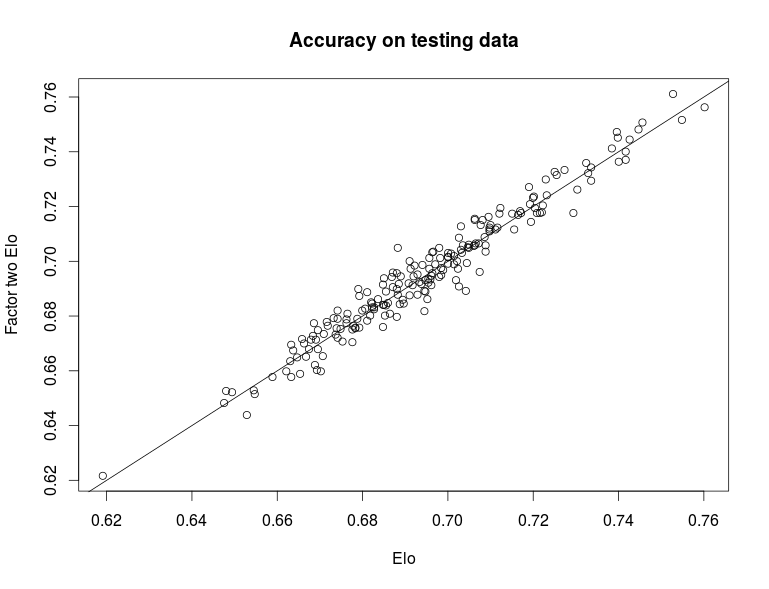
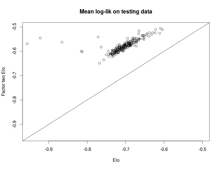
5.1.2.  Rank-four Bradley-Terry-Élő model

These two experiments are designed to compare the rank-four Élő model to the two-factor Élő model when the true log-odds matrix is a rank-four matrix.

The first experiment considers the scenario when all singular values of the true log-odds matrix are big. In this case, the best rank-two approximation to the true log-odds matrix will give a relatively large error because the third and fourth singular components cannot be recovered. The log-odds matrices considered in this experiment takes the following form

$$L=s_{1}\cdot u\cdot v^{\top}+s_{2}\cdot\theta\cdot\underline{1}^{\top}-s_{1}\cdot v\cdot u^{\top}-s_{2}\cdot\underline{1}\cdot\theta^{\top}$$ (16)

, where $s_{1}$ and $s_{2}$ are the two distinct singular values and $\underline{1}$ is parallel to the vector of ones, and vector $\underline{1}$ , $u$, $v$ and $\theta$ are orthonormal. This formulation is based on the decomposition of a real antisymmetric matrix stated in section 4.1.1. The true log-odds matrix $L$ has four non-zero singular values $s_{1}$, $-s_{1}$, $s_{2}$ and $-s_{2}$. In the experiment, $s_{1}=25$ and $s_{2}=24$.

The rest of the data generation and validation setting is the same as the experiments in section 2. The procedure is repeated for 100 times. We applied the paired Wilcoxon test to the 100 paired evaluation results. The test results support the hypothesis that the rank-four Élő model performs significantly better in both metrics (one-sided p-value is less than $2^{-16}$ for both accuracy and mean log-likelihood).

In the second experiment, the components in factors $u$, $v$ and $\theta$ are independently generated from a Gaussian distribution with $\mu=1$ and $\sigma=0.7$. The log-odds matrix is then calculated using equation 12 directly. The factors are no longer orthogonal and the second pair of singular values are often much smaller than the first pair. In this case, the best rank-two approximation will be close to the true log-odds matrix.

The procedure is repeated for 100 times again using the same data generation and validation setting. Paired Wilcoxon test shows rank-four Élő model achieves significantly higher accuracy on the test data (one-sided p-value is 0.015), but the mean log-likelihood is not significantly different (p-value is 0.81).

The results of the above two experiments suggest that the rank-four Élő model will have significantly better performance when the true log-odds matrix has rank four and it cannot be approximated well by a rank-two matrix.

5.1.3.  Regularized log-odds matrix estimation

In the following two experiments, we want to compare the regularized log-odds matrix estimation method with various structured log-odds models.

To carry out regularized log-odds matrix estimation, we need to first get an empirical estimate of log-odds on the training set. Since there are only four matches between any pair of teams in the training data, the estimate of log-odds often turn out to be infinity due to division by zero. Therefore, I introduced a small regularization term in the estimation of empirical winning probability $\hat{p}=\frac{n_{win}+\epsilon}{n_{total}+2\epsilon}$, where $\epsilon$ is set to be 0.01. Then, we obtain the smoothed log-odds matrix by solving the optimization problem described in section 4.4. A sequence of $\lambda$’s are fitted, and the best one is chosen according to the log-likelihood on the evaluation set. The selected model is then evaluated on the testing data set.

Structured log-odds models with different structural assumptions are used for comparison. We consider the Élő model, two-factor Élő model, and rank-four Élő model. For each of the three models, we first tune the hyper-parameter on a further split of training data. Then, we evaluate the models with the best hyper-parameter on the evaluation set and select the best model. Finally, we test the selected model on the test set to produce evaluation metrics. This experiment setting imitates the real application where we need to select the model with best structural assumption.

In order to compare fairly with the trace norm regularization method (which is currently a batch method), the structured log-odds models are trained with batch method and the selected model is not updated during testing.

In the first experiment, it is assumed that the structure of log-odds matrix follows the assumption of the rank-four Élő model. The log-odds matrix is generated using equation (16) with $s_{1}=25$ and $s_{2}=2.5$. The data generation and hypothesis testing procedure remains the same as previous experiments. Paired Wilcoxon test is performed to examine the hypothesis that regularized log-odds model produces higher out-of-sample log-likelihood. The testing result is in favour of this hypothesis (p-value is less than $10^{-10}$).

In the second experiment, it is assumed that the structure of log-odds matrix follows the assumption of the Élő model (section 3.1). The true Élő ratings are generated using a normal distribution with mean $0$ and standard deviation $0.8$. Paired Wilcoxon test shows that the out-of-sample likelihood is somewhat different between the tuned regularized log-odds model and trace norm regularization (two sided p-value = $0.09$).

The experiments show that regularized log-odds estimation can adapt to different structures of the log-odds matrix by varying the regularization parameter. The performance on simulated data set is not worse than the tuned regularized log-odds model.

5.2.  Predictions on the English Premier League

5.2.1.  Description of the data set

The whole data set under investigation consists of English Premier League football matches from 1993-94 to 2014-15 season. There are 8524 matches in total. The data set contains the date of the match, the home team, the away team, and the final scores for both teams. The English Premier League is chosen as a representative as competitive team sports because of its high popularity. In each season, twenty teams will compete against each other using the double round-robin system: each team plays the others twice, once at the home field and once as guest team. The winner of each match scores three championship points. If the match draws, both teams score one point. The final ranking of the teams are determined by the championship points scored in the season. The team with the highest rank will be the champion and the three teams with the lowest rank will move to Division One (a lower-division football league) next season. Similarly, three best performing teams will be promoted from Division One into the Premier League each year. In the data set, 47 teams has played in the Premier League. The data set is retrieved from http://www.football-data.co.uk/.

The algorithms are allowed to use all available information prior to the match to predict the outcome of the match (win, lose, draw).

5.2.2.  Validation setting

In the study of the real data set, we need a proper way to quantify the predictive performance of a model. This is important for two reasons. Firstly, we need to tune the hyper-parameters in the model by performing model validation. The hyper-parameters that bring best performance will be chosen. More importantly, we wish to compare the performance of different types of models scientifically. Such comparison is impossible without a quantitative measure on model performance.

It is a well-known fact that the errors made on the training data will underestimate the model’s true generalization error. The common approaches to assess the goodness of a model include cross validation and bootstrapping [61, 14]. However, both methods assume that the data records are statistically independent. In particular, the records should not contain temporal structure. In the literature, the validation for data with temporal structure is largely an unexplored area. However, the independence assumption is plausibly violated in this study and it is highly likely to affect the result. Hence, we designed an set of ad-hoc validation methods tailored for the current application.

The validation method takes two disjoint data sets, the training data and the testing data. We concatenate the training and testing data into a single data set and partition it into batches $\mathcal{D}$ following the definitions given in 4.3.3. We then run Algorithm 1 on $\mathcal{D}$, but only collect the predictions of matches in the testing data. Those predictions are then compared with the real outcomes in the testing data and various evaluation metrics can be computed.

The exact way to obtain batches $\mathcal{D}$ will depend on the training method we are using. In the experiments, we are mostly interested in the repeated batch re-training method (henceforth batch training method), the on-line training method and the two-stage training method. For these three methods, the batches are defined as follows.

1. Batch training method: the whole training data forms the initial batch $\mathcal{D}_{0}$; the testing data is partitioned into similar-sized batches based on time of the match.

2. On-line training method: all matches are partitioned into similar-sized batches based on time of the match.

3. Two-stage method: the same as batch training method with a different batch size on testing data.

In general, a good validation setting should resemble the usage of the model in practice. Our validation setting guarantees that no future information will be used in making current predictions. It is also naturally related to the training algorithm presented in 4.3.3.

5.2.3.  Prediction Strategy

Most models in this comparative study have tunable hyper-parameters. Those hyper-parameters are tuned using the above validation settings. We split the whole data set into three disjoint subsets, the training set, the tuning set and the testing set. The first match in the training set is the one between Arsenal and Coventry on 1993-08-04, and the first match in the tunning set is the one between Aston Villa and Blackburn on 2005-01-01. The first match in the testing data is the match between Stoke and Fulham on 2010-01-05, and the last match in the testing set is between Stoke and Liverpool on 2015-05-24. The testing set has 2048 matches in total.

In the tuning step, we supply the training set and the tuning set to the validation procedure as the training and testing data. To find the best hyper-parameter, we perform a gird search and the hyper-parameter which achieves the highest out-of-sample likelihood is chosen. In theory, the batch size and epoch size are tunable hyper-parameters, but in the experiments we choose these parameters based on our prior knowledge. For the on-line and two-stage method, each individual match in testing data is regarded as a batch. The epoch size is chosen to be one. This reflects the usual update rule of the conventional Élő ratings: the ratings are updated immediately after the match outcome becomes available. For the batch training method, matches take place in the same quarter of the year are allocated to the same batch.

The model with the selected hyper-parameters is tested using the same validation settings. The training data now consists of both training set and tuning set. The testing data is supplied with the testing set.

This prediction strategy ensures that the training-evaluating-testing split is the same for all training methods, which means that the model will be accessible to the same data set regardless of what training method is being used. This ensures that we can compare different training methods fairly.

All the models will also be compared with a set of benchmarks. The first benchmark is a naive baseline which always predicts home team to win the match. The second benchmark is constructed from the betting odds given by bookmakers. For each match, the bookmakers provide three odds for the three outcomes, win, draw and lose. The betting odds and the probability has the following relationship: $\text{P}=\frac{1}{\text{odds}}$. The probabilities implied by betting odds are used as prediction. However, the bookmaker’s odds will include a vigorish so the implied “probability” does not sum to one. They are normalized by dividing each term with the sum to give the valid probability. The historical odds are also obtained from http://www.football-data.co.uk/.

5.2.4.  Quantitative comparison for the evaluation metrics

We use log-likelihood and accuracy on the testing data set as evaluation metrics. We apply statistical hypothesis testing on the validation results to compare the models quantitatively.

We calculate the log-likelihood on each test case for each model. If we are comparing two models, the evaluation metrics for each test case will form a paired sample. This is because test cases might be correlated with each other and model’s performance is independent given the test case. The paired t-test is used to test whether there is a significant difference in the mean of log-likelihood. We draw independent bootstrap samples with replacement from the log-likelihood values on test cases, and calculate the mean for each sample. We then calculate the 95% confidence interval for the mean log-likelihood based on the empirical quantiles of bootstrapped means [12]. Five thousand bootstrap samples are used to calculate these intervals.

The confidence interval for accuracy is constructed assuming the model’s prediction for each test case, independently, has a probability $p$ to be correct. The reported 95% confidence interval for Binomial random variable is calculated from a procedure first given in Clopper and Pearson [8]. The procedure guarantees that the confidence level is at least 95%, but it may not produce the shortest-length interval.

5.2.5.  Performance of the structured log-odds model

We performed the tunning and validation of the structured log-odds models using the method described in section 5.2.2. The following list shows all models examined by this experiment:

1. The Bradley-Terry-Élő model (section 3.1)

2. Two-factor Bradley-Terry-Élő model (section 4.1)

3. Rank-four Bradley-Terry-Élő model (section 4.1)

4. The Bradley-Terry-Élő model with score difference (section 4.2.3)

5. The Bradley-Terry-Élő model with two additional features (section 4.2.1)

All models include a free parameter for home advantage (see section 4.2.1), and they are also able to capture the probability of a draw (section 4.1). We have introduced two covariates in the fifth model. These two covariates indicate whether the home team or away team is just promoted from Division One this season. We have also tested the trace norm regularized log-odds model, but as indicated in section 4.4 the model still has many limitations for the application to the real data. The validation results are summarized in table 3 and table 4.

The testing results help us understand the following two scientific questions:

1. Which training method brings the best performance to structured log-odds models?

2. Which type of structured log-odds model achieves best performance on the data set?

In order to answer the first question, we test the following hypothesis:

(H1):

Null hypothesis: for a certain model, two-stage training method and online training method produce the same mean out-of-sample log-likelihood. Alternative hypothesis: for a certain model two-stage training method produces a higher mean out-of-sample log-likelihood than online training method.

Here we compare the traditional on-line updating rule with the newly developed two-stage method. The paired t-test is used to assess the above hypotheses. The p-values are shown in table 2. The cell associated with the Élő model with covariates are empty because the online training method does not update the coefficients for features. The first columns of the table gives strong evidence that the two-stage training method should be preferred over online training. All tests are highly significant even if we take into account the issue of multiple testing.

In order to answer the second question, we compare the four new models with the Bradley-Terry-Élő model. The hypothesis is formulated as

(H2):

Null hypothesis: using the best training method, the new model and the Élő model produce the same mean out-of-sample log-likelihood. Alternative hypothesis: using the best training method, the new model produces a higher mean out-of-sample log-likelihood than the Élő model.

The p-values are listed in the last column of table 2. The result also shows that adding more factors in the model does not significantly improve the performance. Neither two-factor model nor rank-four model outperforms the original Bradley-Terry-Élő model on the testing data set. This might provide evidence and justification of using the Bradley-Terry-Élő model on real data set. The model that uses the score difference performs slightly better than the original Bradley-Terry-Élő model. However, the difference in out-of-sample log-likelihood is not statistically significant (the p-value for one-sided test is 0.24 for likelihood). Adding additional covariates about team promotion significantly improves the Bradley-Terry-Élő model.

Type	H1	H2
Élő model	$7.8\times 10^{-5}$	-
Two-factor model	$4.4\times 10^{-14}$	~1
Rank-four model	$9.8\times 10^{-9}$	~1
Score difference	$2.2\times 10^{-16}$	0.235
Élő model with covariates	-	0.002

Table 2: Hypothesis testing on the structured log-odds model. The column “Type” specifies the type of the model; the remaining two columns shows the one-sided p-values for the associated hypothesis

Type	Method	Acc	2.5%	97.5%
Benchmark	Home team win	46.07%	43.93%	48.21%
	Bet365 odds	54.13%	51.96%	56.28%
Élő model	Two-stage	52.40%	50.23%	54.56%
	Online	52.16%	50.00%	54.32%
	Batch	50.58%	48.41%	52.74%
Two-factor model	Two-stage	51.30%	49.13%	53.46%
	Online	50.34%	48.17%	52.50%
	Batch	50.86%	48.69%	53.03%
Rank-four model	Two-stage	51.34%	49.17%	53.51%
	Online	50.34%	48.17%	52.50%
	Batch	50.58%	48.41%	52.74%
Score difference	Two-stage	52.59%	50.42%	54.75%
	Online	47.17%	45.01%	49.34%
	Batch	51.10%	48.93%	53.27%
Élő model with covariates	Two-stage	52.78%	50.61%	54.95%
	Batch	50.86%	48.69%	53.03%
Trace norm regularized model	Batch	45.89%	43.54%	48.21%

Table 3: Structured log-odds model’s accuracy on testing data. The column “Type” specifies the type of the model; the column “Method” specifies the training method. Testing accuracy is given in the column “Acc”. The last two columns gives the 95% confidence interval for testing accuracy

Type	Method	Mean log-loss	2.5%	97.5%
Benchmark	Bet365 odds	-0.9669	-0.9877	-0.9460
Élő model	Two-stage	-0.9854	-1.0074	-0.9625
	Online	-1.0003	-1.0254	-0.9754
	Batch	-1.0079	-1.0314	-0.9848
Two-factor model	Two-stage	-1.0058	-1.0286	-0.9816
	Online	-1.0870	-1.1241	-1.0504
	Batch	-1.0158	-1.0379	-0.9919
Rank-four model	Two-stage	-1.0295	-1.0574	-1.0016
	Online	-1.1024	-1.0638	-1.1421
	Batch	-1.0078	-1.0291	-0.9860
Score difference	Two-stage	-0.9828	-1.0034	-0.9623
	Online	-1.1217	-1.1593	-1.0833
	Batch	-1.0009	-1.0206	-0.9802
Élő model with covariates	Two-stage	-0.9807	-1.0016	-0.9599
	Batch	-1.0002	-1.0204	-0.9798

Table 4: Structured log-odds model’s mean log-likelihood on testing data. The column “Type” specifies the type of the model; the column “Method” specifies the training method. Mean out-of-sample log-likelihood is given in the column “Mean log-loss”. The last two columns gives the 95% confidence interval for mean out-of-sample log-likelihood

5.2.6.  Performance of the batch learning models

This experiment compares the performance of batch learning models. The following list shows all models examined by this experiment:

1. GLM with elastic net penalty using multinomial link function

2. GLM with elastic net penalty using ordinal link function

3. Random forest

4. Dixon-Coles model

The first three models are machine learning models that can be trained on different features. The following features are considered in this experiment:

1. Team id: the identity of home team and away team

2. Ranking: the team’s current ranking in Championship points and goals

3. VS: the percentage of time that home team beats away team in last 3, 6, and 9 matches between them

4. Moving average: the moving average of the following monthly features using lag 3, 6, 12, and 24

   1. percentage of winning at home

   2. percentage of winning away

   3. number of matches at home

   4. number of matches away

   5. championship points earned

   6. number of goals won at home

   7. number of goals won away

   8. number of goals conceded at home

   9. number of goals conceded away

The testing accuracy and out-of-sample log-likelihood are summarized in table 8 and table 9. All models perform better than the baseline benchmark, but no model seems to outperform the state-of-the-art benchmark (betting odds).

We applied statistical testing to understand the following questions

1. Does the GLM with ordinal link function perform better than the GLM with multinomial link function?

2. Which set of features are most useful to make prediction?

3. Which model performs best among GLM, Random forest, and Dixon-Coles model?

For question one, we formulate the hypothesis as:

(H3):

Null hypothesis: for a given set of feature, the GLM with ordinal link function and the GLM with multinomial link function produce the same mean out-of-sample log-likelihood. Alternative hypothesis: for a given set of feature, the mean out-of-sample log-likelihood is different for the two models.

The p-values for these tests are summarized in table 5. In three out of four scenarios, the test is not significant. There does not seem to be enough evidence against the null hypothesis. Hence, we retain our believe that the GLM with different link functions have the same performance in terms of mean out-of-sample log-likelihood.

Features	p-value
Team_id only	0.148
Team_id and ranking	0.035
Team_id and VS	0.118
Team_id and MA	0.121

Table 5: p-values for H3

For question two, we observe that models with the moving average feature have achieved better performance than the same model trained with other features. We formulate the hypothesis as:

(H4):

Null hypothesis: for a given model, the moving average feature and an alternative feature set produce the same mean out-of-sample log-likelihood. Alternative hypothesis: for a given model, the mean out-of-sample log-likelihood is higher for the moving average feature.

The p-values are summarized in table 6. The tests support our believe that the moving average feature set is the most useful one among those examined in this experiment.

Features	GLM1	GLM2
Team_id only	$2.7\times 10^{-12}$	$5.3\times 10^{-8}$
Team_id and ranking	$1.2\times 10^{-9}$	$3.7\times 10^{-6}$
Team_id and VS	0.044	0.004

Table 6: p-values for H4: the column “Features” are the alternative features compared with the moving average features. The next two columns contain the p-values for the GLM with multinomial link function (GLM1) and the GLM with ordinal link function (GLM2)

Finally, we perform comparison among different models. The comparisons are made between the GLM with multinomial link function, Random forest, and Dixon-Coles model. The features used are the moving average feature set. The p-values are summarized in table 7. The tests detect a significant difference between GLM and Random forest, but the other two pairs are not significantly different. We apply the p-value adjustment using Holm’s method in order to control family-wise type-one error [53]. The adjusted p-values are not significant. Hence, we retain our belief that the three models have the same predictive performance in terms of mean out-of-sample log-likelihood.

Comparison	p-value	adjusted
GLM and RF	0.03	0.08
GLM and DC	0.48	0.96
DC and RF	0.54	0.96

Table 7: p-values for model comparison: the column “Comparison” specifies which two models are being compared. “RF” stands for Random forest; “DC” stands for the Dixon-Coles model. The column “p-value” contains the two-sided p-value of the corresponding paired t-test. The column “adjusted” shows the adjusted p-values for multiple testing

Models	Features	Acc	2.5%	97.5%
Benchmark	Home team win	46.07%	43.93%	48.21%
	Bet365 odds	54.13%	51.96%	56.28%
GLM1	Team_id only	50.05%	47.88%	52.22%
	Team_id and ranking	50.62%	48.45%	52.79%
	Team_id and VS	51.25%	49.08%	53.41%
	Team_id and MA	52.69%	50.52%	54.85%
GLM2	Team_id only	50.67%	48.52%	52.82%
	Team_id and ranking	50.24%	48.09%	52.38%
	Team_id and VS	51.92%	49.75%	54.08%
	Team_id and MA	52.93%	50.76%	55.09%
RF	Team_id and MA	52.06%	49.89%	54.23%
Dixon-Coles	-	52.54%	50.40%	54.68%

Table 8: Testing accuracy for batch learning models: The column “Type” specifies the type of the model; “GLM1” refers to the GLM with multinomial link function, and “GLM2” refers to the GLM with ordinal link function. column “Models” specifies the model, and the column “Features” specifies the features used to train the model. Testing accuracy is given in the column “Acc”. The last two columns gives the 95% confidence interval for testing accuracy.

Models	Features	Mean log-loss	2.5%	97.5%
Benchmark	Bet365 odds	-0.9669	-0.9877	-0.9460
GLM1	Team_id only	-1.0123	-1.0296	-0.9952
	Team_id and ranking	-1.0006	-1.0175	-0.9829
	Team_id and VS	-0.9969	-1.0225	-0.9721
	Team_id and MA	-0.9797	-0.9993	-0.9609
GLM2	Team_id only	-1.0184	-1.0399	-0.9964
	Team_id and ranking	-1.0097	-1.0317	-0.9874
	Team_id and VS	-1.0077	-1.0338	-0.9813
	Team_id and MA	-0.9838	-1.0028	-0.9656
RF	Team_id and MA	-0.9885	-1.0090	-0.9683
Dixon-Coles	-	-0.9842	-1.0076	-0.9610

Table 9: out-of-sample log-likelihood for batch learning models: The column “Type” specifies the type of the model; “GLM1” refers to the GLM with multinomial link function, and “GLM2” refers to the GLM with ordinal link function. the column “Models” specifies the model, and the column “Features” specifies the features used to train the model. Mean out-of-sample log-likelihood is given in the column “Mean log-loss”. The last two columns gives the 95% confidence interval for mean out-of-sample log-likelihood.

5.3.  Fairness of the English Premier League ranking

“Fairness” as a concept is statistically undefined and due to its subjectivity is not empirical unless based on peoples’ opinions. The latter may wildly differ and are not systematically accessible from our data set or in general.

Hence we will base our study of the Premier League ranking scheme’s “fairness” on a surrogate derived from the following plausibility considerations: Ranking in any sport should plausibly be based on the participants’ skill in competing in official events of that sport. By definition the outcomes of such events measure the skill in competing at the sport, distorted by a possible component of “chance”. The ranking, derived exclusively from such outcomes, will hence also be determined by the so-measured skills and a component of “chance”.

A ranking system may plausibly be considered fair if the final ranking is only minimally affected by whatever constitutes “chance”, while accurately reflecting the ordering of participating parties in terms of skill, i.e., of being better at the game.

Note that such a definition of fairness is disputable, but it may agree with the general intuition when ranking players of games with a strong chance component such as card or dice games, where cards dealt or numbers thrown in a particular game should, intuitively, not affect a player’s rank, as opposed to the player’s skills of making the best out of a given dealt hand or a dice throw.

Together with the arguments from Section 1.1 which argue for predictability-in-principle surrogating skill, and statistical noise surrogating chance, fairness may be surrogated as the stability of the ranking under the best possible prediction that surrogates the “true odds”. In other words, if we let the same participants, under exactly the same conditions, repeat the whole season, and all that changes is the dealt cards, the thrown numbers, and similar possibly unknown occurrences of “chance”, are we likely to end up with the same ranking as the first time?

While of course this experiment is unlikely to be carried out in real life for most sports, the best possible prediction which is surrogated by the prediction by the best accessible predictive model yields a statistically justifiable estimate for the outcome of such a hypothetical real life experiment.

To obtain this estimate, we consider the as the “best accessible predictive model” the Bradley-Terry-Élő model with features, learnt by the two-stage update rule (see Section 5.2.5), yielding a probabilistic prediction for every game in the season. From these predictions, we may independently sample match outcomes and final rank tables according to the official scoring and ranking rules.

Figure 3 shows estimates for the distribution or ranks of Premier League teams participating in the 2010 season.

Figure 3: Estimated probability for each team participating in the English Premier League season 2010-2011 to obtain the given final rank. Rows are indexed by the different teams in the Premier League of 2010-2011, ordered descendingly by their actual final rank. The x-axis is indexed by the possible ranks from 1 (best) to 20 (worst). The horizontal box-plots are obtained from a Monte-Carlo-sample from 10.000 of the predictive ranking distribution; boxes depict estimates the 25%, 50% and 75% quantiles of the predictive distribution’s Monte Carlo estimate, with whiskers being min/max or 1.5IQR.

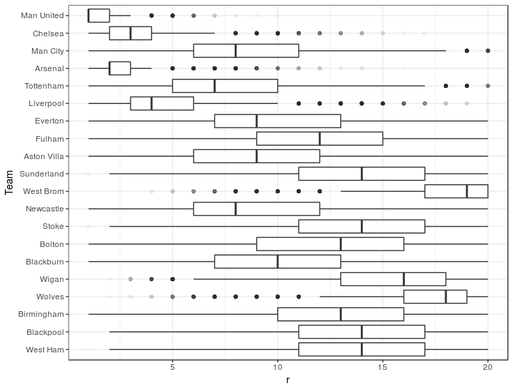
It may be observed that none of the teams, except Manchester United, ends up with the same rank they achieved in reality in more than 50% of the cases. For most teams, the middle 50% are spread over 5 or more ranks, and for all teams, over 2 or more.

From a qualitative viewpoint, the outcome for most teams appears very random, hence the allocation of the final rank seems qualitatively similar to a game of chance notable exceptions being Manchester United and Chelsea whose true final rank is similar to a narrow expected/predicted range. It is also worthwhile noting that Arsenal has been predicted/expected among the first three with high confidence, but eventually was ranked fourth.

The situation is qualitatively similar for later years, though not shown here.

6.  Discussion and Summary

We discuss our findings in the context of our questions regarding prediction of competitive team sports and modelling of English Premier League outcomes, compare Section 1.4

6.1.  Methodological findings

As the principal methodological contribution of this study, we have formulated the Bradley-Terry-Élő model in a joint form, which we have extended to the flexible class of structured log-odds models. We have found structured log-odds models to be potentially useful in the following way:

1. The formulation of the Bradley-Terry-Élő model as a parametric model within a supervised on-line setting solves a number of open issues of the heuristic Élő model, including setting of the K-factor and new players/teams.

2. In synthetic experiments, higher rank Élő models outperform the Bradley-Terry-Élő model in predicting competitive outcomes if the generative truth is higher rank.

3. In real world experiments on the English Premier league, we have found that the extended capability of structured log-odds models to make use of features is useful as it allows better prediction of outcomes compared to not using features.

4. In real world experiments on the English Premier league, we have found that our proposed two-stage training strategy for on-line learning with structured log-odds models is useful as it allows better prediction of outcomes compared to using standard on-line strategies or batch training.

We would like to acknowledge that many of the mentioned suggestions and extensions are already found in existing literature, while, similar to the Bradley-Terry and Élő models in which parsimonious parametric form and on-line learning rule have been separated, those ideas usually appear without being joint to a whole. We also anticipate that the highlighted connections to generalized linear models, low-rank matrix completion and neural networks may prove fruitful in future investigations.

6.2.  Findings on the English Premier League

The main empirical on the English Premier League data may be described as follows.

1. The best predictions, among the methods we compared, are obtained from a structured log-odds model with rank one and added covariates (league promotion), trained via the two-stage strategy. Not using covariates or the batch training method makes the predictions (significantly) worse (in terms of out-of-sample likelihood).

2. All our models and those we adapted from literature were outperformed by the Bet365 betting odds.

3. However, all informed models were very close to each other and the Bet 365 betting odds in performance and not much better than the uninformed baseline of team-independent home team win/draw/lose distribution.

4. Ranking tables obtained from the best accessible predictive model (as a surrogate for the actual process by which it is obtained, i.e., the games proper) are, qualitatively, quite random, to the extent that most teams may end up in wildly different parts of the final table.

While we were able to present a parsimonious and interpretable state-of-art model for outcome prediction for the English Premier League, we found it surprising how little the state-of-art improves above an uninformed guess which already predicts almost half the (win/lose/draw) outcomes correctly, while differences between the more sophisticated methods range in the percents.

Given this, it is probably not surprising that a plausible surrogate for humanity’s “secret” or non-public knowledge of competitive sports prediction, the Bet365 betting odds, is not much better either. Note that this surrogate property is strongly plausible from noticing that offering odds leading to a worse prediction leads to an expected loss in money, hence the market indirectly forces bookmakers to disclose their best prediction. Thus, the continued existence of betting companies hence may lead to the belief that this is possibly rather due to predictions of ordinary people engaged in betting that are worse than uninformed, rather than betting companies’ capability of predicting better. Though we have not extensively studied betting companies empirically, hence this latter belief is entirely conjectural.

Finally, the extent to which the English Premier League is unpredictable raises an important practical concern: influential factors cannot be determined from the data if prediction is impossible, since by recourse to the scientific method assuming an influential factor is one that improves prediction. Our results above allow to definitely conclude only three such factors which are observable, namely a general “good vs bad” quantifier for whatever one may consider as a team’s “skills”, which of the teams is at home, and the fact whether the team is new to the league. As an observation, this is not very deep or unexpected - the surprising aspect is that we were not able to find evidence for more. On a similar note, it is surprising how volatile a team’s position in the final ranking tables seems to be, given the best prediction we were able to achieve.

Hence it may be worthwhile to attempt to understand the possible sources of the observed nigh-unpredictability. On one hand, it can simply be that the correct models are unknown to us and the right data to make a more accurate prediction have been disregarded by us. Though this is made implausible by the observation that the betting odds are similarly bad in predicting, which is somewhat surprising as we have not used much of possibly available detail data such as in-match data and/or player data (which are heavily advertised by commercial data providers these days). On the other hand, unpredictability may be simply due to a high influence of chance inherent to English Premier League games, similar to a game of dice that is not predictable beyond the correct odds. Such a situation may plausibly occur if the “skill levels” of all the participating teams are very close - in an extreme case, where 20 copies of the same team play against each other, the outcome would be entirely up to chance as the skills match exactly, no matter how good or bad these are. Rephrased differently, a game of skill played between two players of equal skill becomes a game of chance. Other plausible causes of the situation is that the outcome a Premier League game is more governed by chance and coincidence than by skills in the first place, or that there are unknown influential factors which are unobserved and possibly distinct from both chance or playing skills. Of course, the mentioned causes do not exclude each other and may be present in varying degrees not determinable from the data considered in this study.

From a team’s perspective, it may hence be interesting to empirically re-evaluate measures that are very costly or resource consuming under the aspect of predictive influence in a similar analysis, say.

6.3.  Open questions

A number of open research questions and possible further avenues of investigation have already been pointed out in-text. We summarize what we believe to be the most interesting avenues for future research:

1. A number of parallels have been highlighted between structured log-odds models and neural networks. It would be interesting to see whether adding layers or other ideas of neural network flavour are beneficial in any application.

2. The correspondence to low-rank matrix completion has motivated a nuclear norm regularized algorithm; yielding acceptable results in a synthetic scenario, the algorithm did not perform better than the baseline on the Premier League data. While this might be due to the above-mentioned issues with that data, general benefits of this alternative approach to structured log-odds models may be worth studying - as opposed to training approaches closer to logistic regression and neural networks.

3. The closeness to low-rank matrix completion also motivates to study identifiability and estimation variance bounds on particular entries of the log-odds matrix, especially in a setting where pairings are not independently or uniformly sampled.

4. While our approach to structured log-odds is inherently parametric, it is not fully Bayesian - though naturally, the benefit of such an approach may be interesting to study.

5. We did not investigate in too much detail the use of features such as player data, and structural restrictions on the feature coefficient matrices and tensors. Doing this, not necessarily in the context of the English Premier League, might be worthwhile, though such a study would have to rely on good sources of added feature data to have any practical impact.

On a more general note, the connection between neural networks and low-rank or matrix factorization principles apparent in this work may also be an interesting direction to explore, not necessarily in a competitive outcome prediction context.

References

- Baio and Blangiardo [2010] Gianluca Baio and Marta Blangiardo. Bayesian hierarchical model for the prediction of football results. Journal of Applied Statistics, 37(2):253–264, 2010.
- Blythe and Király [2015] Duncan AJ Blythe and Franz J Király. Prediction and quantification of individual athletic performance. arXiv preprint arXiv:1505.01147, 2015.
- Bradley and Terry [1952] Ralph Allan Bradley and Milton E Terry. Rank analysis of incomplete block designs: I. the method of paired comparisons. Biometrika, 39(3/4):324–345, 1952.
- Candès and Recht [2009a] Emmanuel J. Candès and Benjamin Recht. Exact matrix completion via convex optimization. Foundations of Computational Mathematics. The Journal of the Society for the Foundations of Computational Mathematics, 9(6):717–772, 2009a. ISSN 1615-3375.
- Candès and Recht [2009b] Emmanuel J Candès and Benjamin Recht. Exact matrix completion via convex optimization. Foundations of Computational mathematics, 9(6):717–772, 2009b.
- Candès and Tao [2010] Emmanuel J. Candès and Terence Tao. The power of convex relaxation: near-optimal matrix completion. Institute of Electrical and Electronics Engineers. Transactions on Information Theory, 56(5):2053–2080, 2010.
- Cattelan et al. [2013] Manuela Cattelan, Cristiano Varin, and David Firth. Dynamic Bradley-Terry modelling of sports tournaments. Journal of the Royal Statistical Society: Series C (Applied Statistics), 62(1):135–150, 2013.
- Clopper and Pearson [1934] Charles J Clopper and Egon S Pearson. The use of confidence or fiducial limits illustrated in the case of the binomial. Biometrika, 26(4):404–413, 1934.
- Constantinou et al. [2012] Anthony C Constantinou, Norman E Fenton, and Martin Neil. pi-football: A bayesian network model for forecasting association football match outcomes. Knowledge-Based Systems, 36:322–339, 2012.
- Coulom [2007] Rémi Coulom. Computing Elo ratings of move patterns in the game of Go. In Computer games workshop, 2007.
- Crowder et al. [2002] Martin Crowder, Mark Dixon, Anthony Ledford, and Mike Robinson. Dynamic modelling and prediction of English football league matches for betting. Journal of the Royal Statistical Society: Series D (The Statistician), 51(2):157–168, 2002.
- Davison and Hinkley [1997] Anthony Christopher Davison and David Victor Hinkley. Bootstrap methods and their application, volume 1. Cambridge university press, 1997.
- Dixon and Coles [1997] Mark J Dixon and Stuart G Coles. Modelling association football scores and inefficiencies in the football betting market. Journal of the Royal Statistical Society: Series C (Applied Statistics), 46(2):265–280, 1997.
- Efron and Tibshirani [1997] Bradley Efron and Robert Tibshirani. Improvements on cross-validation: the 632+ bootstrap method. Journal of the American Statistical Association, 92(438):548–560, 1997.
- Élő [1978] Árpád I Élő. The rating of chessplayers, past and present. Arco Pub., 1978.
- Eves [1980] Howard Whitley Eves. Elementary matrix theory. Courier Corporation, 1980.
- FIFA [2016] FIFA. FIFA/Coca-Cola world ranking: Women’s ranking procedure. http://www.fifa.com/fifa-world-ranking/procedure/women.html, 2016. Accessed: 2016-05-30.
- Firth and Turner [2012] David Firth and Heather L Turner. Bradley-Terry models in r: the bradleyterry2 package. Journal of Statistical Software, 48(9), 2012.
- Glickman [1995] Mark E Glickman. A comprehensive guide to chess ratings. American Chess Journal, 3:59–102, 1995.
- Glickman and Stern [1998] Mark E Glickman and Hal S Stern. A state-space model for national football league scores. Journal of the American Statistical Association, 93(441):25–35, 1998.
- Goddard [2005] John Goddard. Regression models for forecasting goals and match results in association football. International Journal of forecasting, 21(2):331–340, 2005.
- Griffith [1949] Richard M Griffith. Odds adjustments by american horse-race bettors. The American Journal of Psychology, 62(2):290–294, 1949.
- Hucaljuk and Rakipović [2011] Josip Hucaljuk and Alen Rakipović. Predicting football scores using machine learning techniques. In MIPRO, 2011 Proceedings of the 34th International Convention, pages 1623–1627. IEEE, 2011.
- Hunter [2004] David R Hunter. MM algorithms for generalized Bradley-Terry models. Annals of Statistics, pages 384–406, 2004.
- Hyndman and Athanasopoulos [2014] Rob J Hyndman and George Athanasopoulos. Forecasting: principles and practice. OTexts, 2014.
- Isaacs [1953] Rufus Isaacs. Optimal horse race bets. The American Mathematical Monthly, 60(5):310–315, 1953.
- Jewson [2004] Stephen Jewson. The problem with the brier score. arXiv preprint physics/0401046, 2004.
- Johnson et al. [1997] Norman Lloyd Johnson, Samuel Kotz, and Narayanaswamy Balakrishnan. Discrete multivariate distributions, volume 165. Wiley New York, 1997.
- Kampakis and Adamides [2014] Stylianos Kampakis and Andreas Adamides. Using twitter to predict football outcomes. arXiv preprint arXiv:1411.1243, 2014.
- Karlis and Ntzoufras [2003] Dimitris Karlis and Ioannis Ntzoufras. Analysis of sports data by using bivariate poisson models. Journal of the Royal Statistical Society: Series D (The Statistician), 52(3):381–393, 2003.
- Karlis and Ntzoufras [2009] Dimitris Karlis and Ioannis Ntzoufras. Bayesian modelling of football outcomes: using the Skellam’s distribution for the goal difference. IMA Journal of Management Mathematics, 20(2):133–145, 2009.
- Keshavan et al. [2010] Raghunandan H. Keshavan, Andrea Montanari, and Sewoong Oh. Matrix completion from a few entries. Institute of Electrical and Electronics Engineers. Transactions on Information Theory, 56(6):2980–2998, 2010.
- Király et al. [2015] Franz J Király, Louis Theran, and Ryota Tomioka. The algebraic combinatorial approach for low-rank matrix completion. The Journal of Machine Learning Research, 16(1):1391–1436, 2015.
- Kocherlakota and Kocherlakota [1992] Subrahmaniam Kocherlakota and Kathleen Kocherlakota. Bivariate discrete distributions. Wiley Online Library, 1992.
- Lasek et al. [2013] Jan Lasek, Zoltán Szlávik, and Sandjai Bhulai. The predictive power of ranking systems in association football. International Journal of Applied Pattern Recognition, 1(1):27–46, 2013.
- Liu and Lai [2010] Brian Liu and Patrick Lai. Beating the ncaa football point spread, 2010.
- Maher [1982] Michael J Maher. Modelling association football scores. Statistica Neerlandica, 36(3):109–118, 1982.
- McCullagh [1980] Peter McCullagh. Regression models for ordinal data. Journal of the royal statistical society. Series B (Methodological), pages 109–142, 1980.
- McCullagh and Nelder [1989] Peter McCullagh and John A Nelder. Generalized linear models, volume 37. CRC press, 1989.
- Meka et al. [2009] Raghu Meka, Prateek Jain, and Inderjit S. Dhillon. Guaranteed rank minimization via singular value projection. arXiv e-prints, 2009. arXiv:0909.5457.
- Mishra et al. [2013] Bamdev Mishra, Gilles Meyer, Francis Bach, and Rodolphe Sepulchre. Low-rank optimization with trace norm penalty. SIAM Journal on Optimization, 23(4):2124–2149, 2013.
- Negahban and Wainwright [2011] Sahand Negahban and Martin J. Wainwright. Estimation of (near) low-rank matrices with noise and high-dimensional scaling. Annals of Statistics, 39(2), 2011.
- Odachowski and Grekow [2012] Karol Odachowski and Jacek Grekow. Using bookmaker odds to predict the final result of football matches. In Knowledge Engineering, Machine Learning and Lattice Computing with Applications, pages 196–205. Springer, 2012.
- Paterek [2012] Arkadiusz Paterek. Predicting movie ratings and recommender systems: A 195-page monograph on machine learning, recommender systems, and the Netflix Prize. Arkadiusz Paterek, 2012.
- Pollard [1986] Richard Pollard. Home advantage in soccer: A retrospective analysis. Journal of Sports Sciences, 4(3):237–248, 1986.
- Pong et al. [2010] Ting Kei Pong, Paul Tseng, Shuiwang Ji, and Jieping Ye. Trace norm regularization: Reformulations, algorithms, and multi-task learning. SIAM Journal on Optimization, 20(6):3465–3489, 2010.
- Premier League [2016] The Premier League. About the Premier League. http://www.premierleague.com/en-gb/about/the-worlds-most-watched-league.html, 2016. Accessed: 2016-06-26.
- Rao and Kupper [1967] PV Rao and Lawrence L Kupper. Ties in paired-comparison experiments: A generalization of the Bradley-Terry model. Journal of the American Statistical Association, 62(317):194–204, 1967.
- Resnick [2013] Sidney I Resnick. Extreme values, regular variation and point processes. Springer, 2013.
- Rue and Salvesen [2000] Havard Rue and Oyvind Salvesen. Prediction and retrospective analysis of soccer matches in a league. Journal of the Royal Statistical Society: Series D (The Statistician), 49(3):399–418, 2000.
- Schmidhuber [2015] Jürgen Schmidhuber. Deep learning in neural networks: An overview. Neural Networks, 61:85–117, 2015.
- Silver [2014] Nate Silver. Introducing NFL Elo ratings. https://fivethirtyeight.com/datalab/introducing-nfl-elo-ratings/, 2014. Accessed: 2016-05-30.
- Sinclair et al. [2013] Jonathan K Sinclair, Paul J Taylor, and Sarah Jane Hobbs. Alpha level adjustments for multiple dependent variable analyses and their applicability – a review. Int J Sports Sci Eng, 7(1):17–20, 2013.
- Skellam [1945] John G Skellam. The frequency distribution of the difference between two Poisson variates belonging to different populations. Journal of the Royal Statistical Society. Series A (General), 109(Pt 3):296–296, 1945.
- So and Ye [2007] Anthony Man-Cho So and Yinyu Ye. Theory of semidefinite programming for sensor network localization. Mathematical Programming, 109(2-3):367–384, 2007.
- Srebro [2004] Nathan Srebro. Learning with matrix factorizations. PhD thesis, Massachusetts Institute of Technology, 2004.
- Srebro and Shraibman [2005a] Nathan Srebro and Adi Shraibman. Rank, trace-norm and max-norm. In Proceedings of the 18th Annual Conference on Learning Theory (COLT), pages 545–560. Springer, 2005a.
- Srebro and Shraibman [2005b] Nathan Srebro and Adi Shraibman. Rank, trace-norm and max-norm. In International Conference on Computational Learning Theory, pages 545–560. Springer, 2005b.
- Srebro et al. [2004] Nathan Srebro, Jason Rennie, and Tommi S Jaakkola. Maximum-margin matrix factorization. In Advances in neural information processing systems, pages 1329–1336, 2004.
- Stanescu [2011] Marius Stanescu. Rating systems with multiple factors, 2011. Master’s thesis, School of Informatics, Univ. of Edinburgh, Edinburgh, UK.
- Stone [1974] Mervyn Stone. Cross-validatory choice and assessment of statistical predictions. Journal of the Royal Statistical Society. Series B (Methodological), pages 111–147, 1974.
- Vandenberghe and Boyd [1996] Lieven Vandenberghe and Stephen Boyd. Semidefinite programming. SIAM review, 38(1):49–95, 1996.
- Vounou et al. [2010] Maria Vounou, Thomas E Nichols, Giovanni Montana, Alzheimer’s Disease Neuroimaging Initiative, et al. Discovering genetic associations with high-dimensional neuroimaging phenotypes: a sparse reduced-rank regression approach. Neuroimage, 53(3):1147–1159, 2010.