Structural, thermodynamic, and transport properties of CH₂ plasma in the two-temperature regime

Abstract

This paper covers calculation of radial distribution functions, specific energy and static electrical conductivity of CH₂ plasma in the two-temperature regime. The calculation is based on the quantum molecular dynamics, density functional theory and the Kubo-Greenwood formula.

The properties are computed at 5 kK $\leq T_{i}\leq T_{e}\leq 40$ kK and $\rho=0.954$ g/cm³ and depend severely on the presence of chemical bonds in the system. Chemical compounds exist at the lowest temperature $T_{i}=T_{e}=5$ kK considered; they are destroyed rapidly at the growth of $T_{i}$ and slower at the increase of $T_{e}$.

A significant number of bonds are present in the system at 5 kK $\leq T_{i}\leq T_{e}\leq 10$ kK. The destruction of bonds correlates with the growth of specific energy and static electrical conductivity under these conditions.

I Introduction

Carbon-hydrogen plastics are widely used nowadays in various experiments on the interaction of intense energy fluxes with matter. One of these fruitful applications is described in the paper by Povarnitsyn et al.:Povarnitsyn et al. (2013) a polyethylene film may be used to block the prepulse, and thereby, to improve the contrast of an intense laser pulse.

Two types of prepulse are considered:Povarnitsyn et al. (2013) nanosecond (intensity $I_{\mathrm{ns}}=10^{13}$ W/cm²; duration $t_{\mathrm{ns}}=2$ ns) and picosecond ($I_{\mathrm{ps}}=10^{15}$ W/cm²; $t_{\mathrm{ps}}=20$ ps) ones . Both prepulses absorbed by the film produce the state of plasma with an electron temperature $T_{e}$ exceeding an ion temperature $T_{i}$. The conditions with $T_{e}>T_{i}$ are often called a two-temperature ($2T$) regime. The appearance of the $2T$-state may be explained as follows. The absorption of laser radiation by electrons assists the creation of the $2T$-state: the larger laser intensity $I$, the faster $T_{e}-T_{i}$ grows. The electron-phonon coupling destroys the $2T$-state: the larger electron-phonon coupling constant $G$, the faster $T_{e}-T_{i}$ decreases. Thus if the prepulse intensity $I$ is great enough, the $2T$-state with considerable $T_{e}-T_{i}$ may be created.

The action of the prepulse may be described quantitatively using numerical simulation Povarnitsyn et al. (2013, 2015). Modelling Povarnitsyn et al. (2013) shows, that after a considerable part of the nanosecond prepulse has been absorbed, the following conditions are obtained: relative change of density $\rho/\rho_{0}=10^{-4}$–$10^{-2}$, $T_{i}\sim 400$ kK, $T_{e}\sim 4\cdot 10^{3}$ kK. A number of matter properties are required to simulate the action of the prepulse. Particularly, an equation of state, a complex dielectric function and a thermal conductivity coefficient should be known. Paper Povarnitsyn et al. (2013) employs rather rough models of matter properties. Therefore, the need for better knowledge of plasma properties arises.

The matter properties should be known for all the states of the system: from the ambient conditions to the extreme parameters specified above. The required properties may be calculated via various techniques, including: the average atom model Ovechkin et al. (2014), the chemical plasma model Apfelbaum (2016) and quantum molecular dynamics (QMD). None of these methods may yield data for all conditions emerging under the action of the prepulse. The QMD technique is a powerful tool for the calculation of properties in the warm dense matter regime (rather high densities and moderate temperatures).

QMD is widely used for the calculation of thermodynamic properties, including equation of state Wang and Zhang (2013), shock Hugoniots Wang et al. (2013); Minakov et al. (2014) and melting curves Minakov and Levashov (2015). A common approach to obtain electronic transport and optical properties from a QMD simulation is to use the Kubo-Greenwood formula (KG). Here the transport properties encompass static electrical conductivity and thermal conductivity, whereas the optical properties include dynamic electrical conductivity, complex dieletric function, complex refraction index and reflectivity. The QMD+KG technique became particularly widespread after the papers Desjarlais et al. (2002); Recoules and Crocombette (2005). Some of the most recent QMD+KG calculations address transport and optical properties of deuterium Hu et al. (2015), berillium Li et al. (2015), xenon Norman et al. (2015) and copper Migdal et al. (2016).

Carbon-hydrogen plasma has also been explored by the QMD technique recently. Pure C_mH_n plasma (carbon and hydrogen ions are the only ions present in the system) was considered in papers Mattsson et al. (2010); Wang et al. (2011); Lambert and Recoules (2012); Hamel et al. (2012); Chantawansri et al. (2012); Hu et al. (2014); Danel and Kazandjian (2015). Other works Horner et al. (2010); Magyar et al. (2015); Huser et al. (2015); Colin-Lalu et al. (2015) study the influence of dopants. Transport and optical properties of carbon-hydrogen plasma were investigated in papers Horner et al. (2010); Wang et al. (2011); Lambert and Recoules (2012); Hu et al. (2014); Huser et al. (2015). Some of the cited works are discussed in more detail in our previous work Knyazev and Levashov (2015).

None of the papers mentioned above studies the influence of the $2T$-state on the properties of carbon-hydrogen plasma. The lack of such data was the first reason stimulating this work. In this paper we calculate specific energy and static electrical conductivity of CH₂ plasma in the $2T$-state via the QMD+KG technique. The plasma of CH₂ composition corresponds to polyethylene heated by laser radiation. In this work the properties are calculated at the normal density of polyethylene $\rho=0.954$ g/cm³ and at temperatures 5 kK $\leq T_{i}\leq T_{e}\leq 40$ kK. These conditions correspond to the very beginning of the prepulse action; the temperatures after the prepulse are much larger. However, the beginning of the prepulse action should be also simulated carefully, since the spacial distribution of plasma at the initial stage influences the whole following process dramatically. Thus we have to know the properties of CH₂ plasma even for such moderate temperatures.

Properties of CH₂ plasma in the one-temperature ($1T$) case $T_{i}=T_{e}$ were investigated in our previous work Knyazev and Levashov (2015). The properties were calculated at $\rho=0.954$ g/cm³ and at temperatures 5 kK $\leq T_{i}=T_{e}=T\leq 100$ kK.

The most interesting results obtained in Knyazev and Levashov (2015) concern specific heat capacity and static electrical conductivity of CH₂ plasma. The specific heat capacity $\mathcal{C}_{v}(T)$ decreases at 5 kK $\leq T\leq 15$ kK and increases at 15 kK $\leq T\leq 100$ kK. The decrease of $\mathcal{C}_{v}(T)$ corresponds to the concave shape of the temperature dependence of specific energy $\mathcal{E}(T)$. The temperature dependence of the static electrical conductivity $\sigma_{1_{\mathrm{DC}}}(T)$ demonstrates step-like behavior: it grows rapidly at 5 kK $\leq T\leq 10$ kK and remains almost constant at 20 kK $\leq T\leq 60$ kK. Similar step-like curves for reflectivity along principal Hugoniots of carbon-hydrogen plastics were obtained in the previous works Wang et al. (2011); Hu et al. (2014); Huser et al. (2015).

The second reason for the current work is the drive to explain the obtained $\mathcal{E}(T)$ and $\sigma_{1_{\mathrm{DC}}}(T)$ dependences. During a $2T$-calculation one of the temperatures ($T_{i}$ or $T_{e}$) is kept fixed while the other one is varied. This helps to understand better the influence of $T_{i}$ and $T_{e}$ on the one-temperature $\mathcal{E}(T)$ and $\sigma_{1_{\mathrm{DC}}}(T)$ dependences.

The structure of our paper is quite straightfoward. Sec. II contains a brief description of the computation method. The technical parameters used during the calculation are available in Sec. III. The results on $\mathcal{E}$ and $\sigma_{1_{\mathrm{DC}}}$ of CH₂ plasma are presented in Sec. IV. The discussion of the results based on the investigation of radial distribution functions (RDFs) is also available in Sec. IV.

II Computation technique

The computation technique is based on quantum molecular dynamics, density functional theory (DFT) in its Kohn-Sham formulation and the Kubo-Greenwood formula. The method of calculation for $1T$ case was described in detail in our previous work Knyazev and Levashov (2013) and the papers Desjarlais et al. (2002); Recoules and Crocombette (2005). An example of $2T$-calculation is present in our previous paper Knyazev and Levashov (2014). Here we will give only a brief overview of the employed technique.

The computation method consists of three main stages: QMD simulation, precise resolution of the band structure and the calculation via the KG formula.

At the first stage $N_{C}$ atoms of carbon and $N_{H}=2N_{C}$ atoms of hydrogen are placed in a supercell with periodic boundary conditions. The total number of atoms $N_{\mathrm{at}}=N_{C}+N_{H}$ may be varied. At the given $N_{\mathrm{at}}$ the size of the supercell is chosen to yield the correct density $\rho$. Ions are treated classically. The ions of carbon and hydrogen are placed in the random nodes of the auxiliary simple cubic lattice. We have discussed the choice of the initial ionic configuration and performed an overview of the works on this issue previously Knyazev and Levashov (2015). Then the QMD simulation is performed.

The electronic structure is calculated at each QMD step within the Born-Oppenheimer approximation: electrons totally adjust to the current ionic configuration. This calculation is performed within the framework of DFT: the finite-temperature Kohn-Sham equations are solved. The occupation numbers used during their solution are set by the Fermi-Dirac distribution. The latter includes the electron temperature $T_{e}$; this is how the calculation depends on $T_{e}$.

The forces acting on each ion from the electrons and other ions are calculated at every step. The Newton equations of motion are solved for the ions using these forces; thus the ionic trajectories are calculated. Additional forces are also acting on the ions from the Nosé thermostat. These forces are used to bring the total kinetic energy of ions $E_{i}^{\mathrm{kin}}(t)$ to the average value $\frac{3}{2}(N_{\mathrm{at}}-1)kT_{i}$ after some period of simulation; here $k$ is the Boltzmann constant. This is how the calculation depends on $T_{i}$. QMD simulation is performed using the Vienna ab initio simulation package (VASP) Kresse and Hafner (1993, 1994); Kresse and Furthmüller (1996).

The ionic trajectories and the temporal dependence of the energy without the kinetic contribution of ions $[E-E_{i}^{\mathrm{kin}}](t)$ are obtained during the QMD simulation. The system comes to a two-temperature equilibrium state after some number of QMD steps is performed. In this state equilibrium exists only within the electronic and ionic subsystems separately. The exchange of energy between electrons and ions is absent, since the Born-Oppenheimer approximation is used during the QMD simulation. $[E-E_{i}^{\mathrm{kin}}](t)$ fluctuates around its average value in this two-temperature equilibrium state. A significant number of sequential QMD steps corresponding to the two-temperature equilibrium state are chosen. $[E-E_{i}^{\mathrm{kin}}](t)$ dependence is averaged over these sequential steps; thus the thermodynamic value $[E-E_{i}^{\mathrm{kin}}]$ is obtained. If the dependence on time is not mentioned, $[E-E_{i}^{\mathrm{kin}}]$ denotes the thermodynamic value of the energy without the kinetic contribution of ions here. The thermodynamic value is then divided by the mass of the supercell; this specific energy is designated by $[\mathcal{E}-\mathcal{E}_{i}^{\mathrm{kin}}]$.

The total energy of electrons and ions $E$ may also be calculated. However, these data are not presented in this paper to understand better the temperature dependence of energy. The thermodynamic value of $E_{i}^{\mathrm{kin}}$ is $\frac{3}{2}(N_{\mathrm{at}}-1)kT_{i}$ because of the interaction with the Nosé thermostat. Thus $E_{i}^{\mathrm{kin}}$ depends only on $T_{i}$ in a rather simple way: $E_{i}^{\mathrm{kin}}(T_{i})\sim T_{i}$. $[E-E_{i}^{\mathrm{kin}}]$ may depend both on $T_{i}$ and $T_{e}$ in a complicated manner. The addition of $E_{i}^{\mathrm{kin}}(T_{i})$ will just obscure the $[E-E_{i}^{\mathrm{kin}}](T_{i},T_{e})$ dependence. If necessary, the total energy may be reconstructed easily.

The separate configurations corresponding to the two-temperature equilibrium state are selected for the calculation of static electrical conductivity and optical properties. At the second stage the precise resolution of the band structure is performed for these separate configurations. The same Kohn-Sham equations as during the first stage are solved, though the technical parameters yielding a higher precision may be used. At this stage the Kohn-Sham eigenvalues, corresponding wave functions and occupation numbers are obtained. The precise resolution of the band structure is performed with the VASP package. Then the obtained wave functions are used to calculate the matrix elements of the nabla operator; this is done using the optics.f90 module of the VASP package.

At the third stage the real part of the dynamic electrical conductivity $\sigma_{1}(\omega)$ is calculated via the KG formula presented in our previous paper Knyazev and Levashov (2013); the formula includes matrix elements of the nabla operator, energy eigenvalues and occupation numbers calculated during the precise resolution of the band structure. We have created a parallel program to perform a calculation according to the KG formula, it uses data obtained by the VASP as input information. $\sigma_{1_{j}}(\omega)$ is obtained for each of the selected ionic configurations. These $\sigma_{1_{j}}(\omega)$ curves are then averaged to get the final $\sigma_{1}(\omega)$. The static electrical conductivity $\sigma_{1_{\mathrm{DC}}}$ is calculated via an extrapolation of $\sigma_{1}(\omega)$ to zero frequency. The simple linear extrapolation described in Knyazev and Levashov (2013) is used.

A number of sequential ionic configurations corresponding to the $2T$ equilibrium stage of the QMD simulation are also used to calculate RDFs. C-C, C-H and H-H RDFs are calculated with the Visual Molecular Dynamics program (VMD) Humphrey et al. (1996).

III Technical parameters

The QMD simulation was performed with 120 atoms in the computational supercell (40 carbon atoms and 80 hydrogen atoms). At the initial moment the ions were placed in the random nodes of the auxiliary simple cubic lattice (discussed in Knyazev and Levashov (2015)). Then 15000 steps of the QMD simulation were performed, one step corresponded to 0.2 fs. Thus the evolution of the system during 3 ps was tracked. The calculation was run in the framework of the local density approximation (LDA) with the Perdew–Zunger parametrization (set by Eqs. (C3), (C5) and Table XII, the first column, of paperPerdew and Zunger (1981)). We have applied the pseudopotentials of the projector augmented-wave (PAW Blöchl (1994); Kresse and Joubert (1999)) type both for carbon and hydrogen. The PAW pseudopotential for carbon took 4 electrons into account ($2s^{2}2p^{2}$); the core radius $r_{c}$ was equal to $1.5a_{B}$, here $a_{B}$ is the Bohr radius. The PAW pseudopotential for hydrogen allowed for 1 electron per atom ($1s^{1}$), $r_{c}=1.1a_{B}$. The QMD simulation was performed with 1 k-point in the Brillouin zone ($\Gamma$-point) and with the energy cut-off $E_{\mathrm{cut}}=300$ eV. All the bands with occupation numbers larger than $5\times 10^{-6}$ were taken into account. The section of the QMD simulation corresponding to 0.5 ps $\leq t\leq 2.5$ ps was used to average the temporal dependence $[E-E_{i}^{\mathrm{kin}}](t)$.

We have chosen 15 ionic configurations for the further calculation of $\sigma_{1_{\mathrm{DC}}}$. The first of these configurations corresponded to $t=0.2$ ps, the time span between the neighboring configurations also was $0.2$ ps. The band structure was calculated one more time for these selected configurations. The exchange-correlation functional, pseudopotential, number of k-points and energy cut-off were the same as during the QMD simulation. Additional unoccupied bands were taken into account, they spanned an energy range of 40 eV.

The $\sigma_{1_{j}}(\omega)$ curves were calculated for the selected ionic configurations at 0.005 eV $\leq\omega\leq 40$ eV with a frequency step 0.005 eV. The $\delta$-function in the KG formula was broadened by the GaussianDesjarlais et al. (2002) function with the standard deviation of 0.2 eV.

The RDFs were calculated for the section of the QMD simulation corresponding to 1.8002 ps $\leq t\leq 2$ ps for the distances 0.05 Å$\leavevmode\nobreak\ \leq r\leq 4$ Å with the step of $\Delta r=0.1$ Å.

For computational results to be reliable, the convergence by technical parameters should be checked. However, the full investigation of convergence is very time-consuming. In our previous works we have performed full research on convergence for aluminum Knyazev and Levashov (2013) and partial—for CH₂ plasma Knyazev and Levashov (2015). It was shown Knyazev and Levashov (2013), that the number of atoms $N_{\mathrm{at}}$ and the number of k-points $N_{\mathbf{k}}$ during the precise resolution of the band structure contribute to the error of $\sigma_{1_{\mathrm{DC}}}$ most of all; the effect of these parameters is of the same order of magnitude. The size effects in CH₂ plasma were investigated earlier:Knyazev and Levashov (2015) the results for $\sigma_{1_{\mathrm{DC}}}$ were the same within several percents for 120 and 249 atoms in the supercell. In our current paper we use the same moderate $N_{\mathrm{at}}$ and $N_{\mathbf{k}}$ values as in Knyazev and Levashov (2015). This introduces a small error to our results, but speeds up computations considerably.

IV Results

The following types of calculations were performed:

• one-temperature case with $T_{i}=T_{e}=T$;

• $2T$-computations at fixed $T_{i}$ and varied $T_{e}$, so that $T_{e}\geq T_{i}$;

• $2T$-computations at fixed $T_{e}$ and varied $T_{i}$, so that $T_{i}\leq T_{e}$.

The overall range of temperatures under consideration is 5 kK $\leq T_{i}\leq T_{e}\leq 40$ kK. The calculations were performed at fixed $\rho=0.954$ g/cm³.

These calculations allow us to obtain the dependence of a quantity $f$ both on $T_{i}$ and $T_{e}$: $f(T_{i},T_{e})$. Here $f$ may stand for $[\mathcal{E}-\mathcal{E}_{i}^{\mathrm{kin}}]$ or $\sigma_{1_{\mathrm{DC}}}$. The one-temperature dependences $f(T)|_{T_{i}=T_{e}}$ were investigated previously Knyazev and Levashov (2015). In this paper we also present $f(T_{e})|_{T_{i}=\mathrm{const}}$ and $f(T_{i})|_{T_{e}=\mathrm{const}}$. The slope of $f(T_{e})|_{T_{i}=\mathrm{const}}$ equals $\left(\frac{\partial f}{\partial T_{e}}\right)_{T_{i}}$; the slope of $f(T_{i})|_{T_{e}=\mathrm{const}}$—$\left(\frac{\partial f}{\partial T_{i}}\right)_{T_{e}}$. The slope of $f(T)|_{T_{i}=T_{e}}$ may be designated by $\left(\frac{\partial f}{\partial T}\right)_{T_{i}=T_{e}}$. Then the following equation is valid:

$$\left(\frac{\partial f}{\partial T}\right)_{T_{i}=T_{e}}=\bigg{[}\left(\frac{\partial f}{\partial T_{e}}\right)_{T_{i}}+\left(\frac{\partial f}{\partial T_{i}}\right)_{T_{e}}\bigg{]}_{T_{i}=T_{e}}.$$ (1)

If we compare the contributions of $\left(\frac{\partial f}{\partial T_{e}}\right)_{T_{i}}$ and $\left(\frac{\partial f}{\partial T_{i}}\right)_{T_{e}}$ to $\left(\frac{\partial f}{\partial T}\right)_{T_{i}=T_{e}}$ we can understand, whether $f(T)|_{T_{i}=T_{e}}$ dependence is mainly due to the change of $T_{i}$ or $T_{e}$.

Now we can define the volumetric mass-specific heat capacity without the kinetic contribution of ions ${[\mathcal{C}_{v}-\mathcal{C}_{v\leavevmode\nobreak\ i}^{\mathrm{kin}}]}$ for the one-temperature case $T_{i}=T_{e}=T$:

$$[\mathcal{C}_{v}-\mathcal{C}_{v\leavevmode\nobreak\ i}^{\mathrm{kin}}]=\left(\frac{\partial[\mathcal{E}-\mathcal{E}_{i}^{\mathrm{kin}}]}{\partial T}\right)_{T_{i}=T_{e}}.$$ (2)

Then Eq. (1) for $f=[\mathcal{E}-\mathcal{E}_{i}^{\mathrm{kin}}]$ may be written as:

$$[\mathcal{C}_{v}-\mathcal{C}_{v\leavevmode\nobreak\ i}^{\mathrm{kin}}]=\bigg{[}\left(\frac{\partial[\mathcal{E}-\mathcal{E}_{i}^{\mathrm{kin}}]}{\partial T_{e}}\right)_{T_{i}}+\\ +\left(\frac{\partial[\mathcal{E}-\mathcal{E}_{i}^{\mathrm{kin}}]}{\partial T_{i}}\right)_{T_{e}}\bigg{]}_{T_{i}=T_{e}}.$$ (3)

Radial distribution functions were calculated for two cases only:

• one-temperature case 5 kK $\leq T_{i}=T_{e}=T\leq 40$ kK (Fig. 1(b), Fig. 2(b), Fig. 3(b));

• two-temperature case $T_{i}=5$ kK; 5 kK $\leq T_{e}\leq 40$ kK (Fig. 1(a), Fig. 2(a), Fig. 3(a)).

Carbon-carbon (Fig. 1), carbon-hydrogen (Fig. 2) and hydrogen-hydrogen (Fig. 3) RDFs are presented.

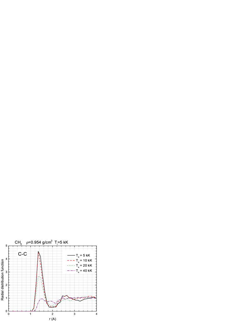
a)  b) 

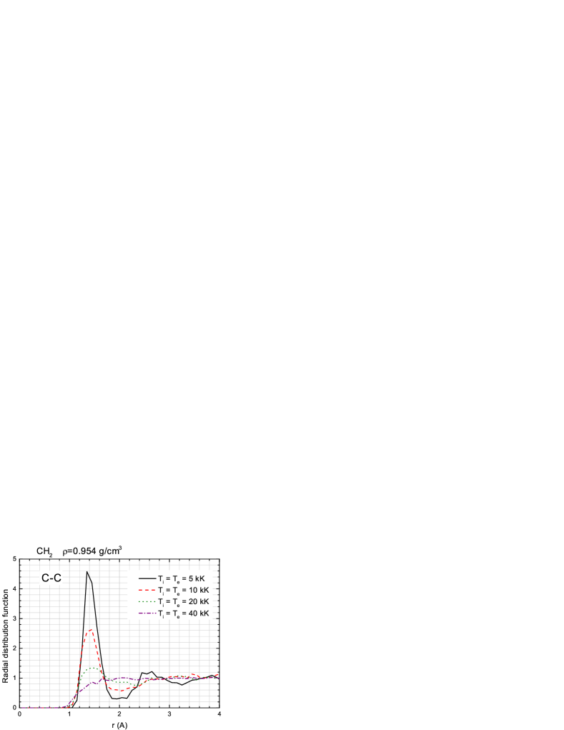
Figure 1: C-C radial distribution functions at various temperatures. (a) Two-temperature case: $T_{i}$ is kept fixed at 5 kK; $T_{e}$ is varied. (b) One-temperature case: $T_{i}$ and $T_{e}$ are varied simultaneously, so that $T_{i}=T_{e}=T$. Lines of different types correspond to different temperatures.

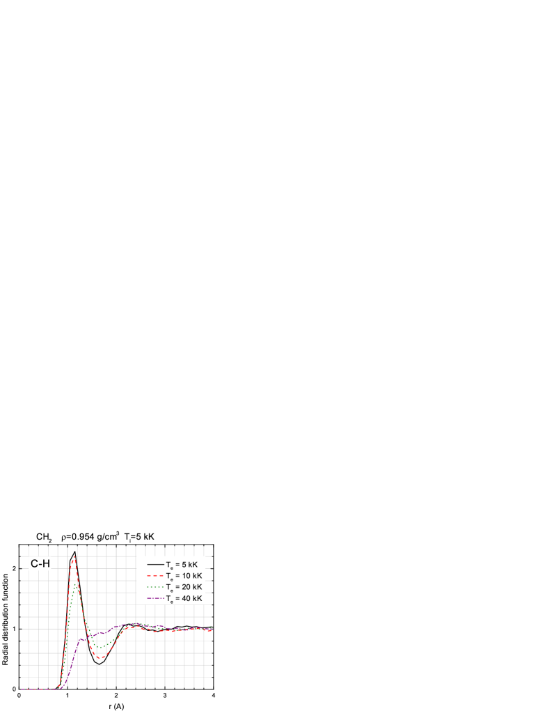
a)  b) 

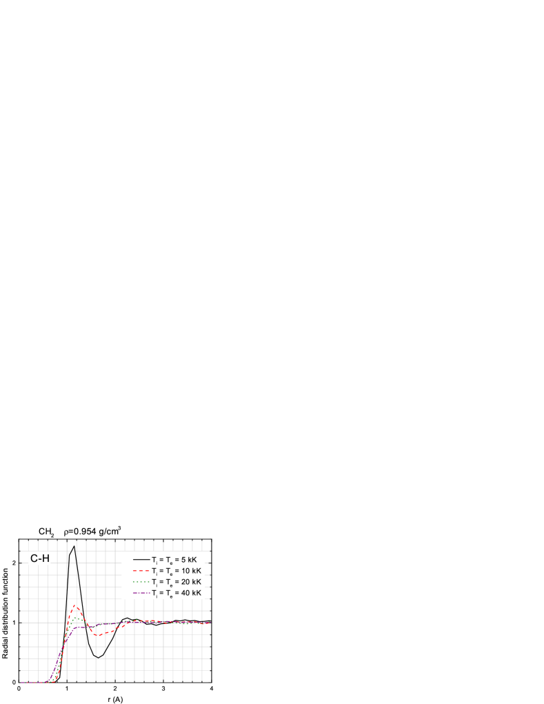
Figure 2: Same as Fig. 1 but for C-H radial distribution functions.

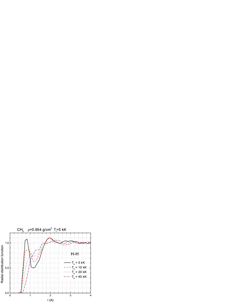
a)  b) 

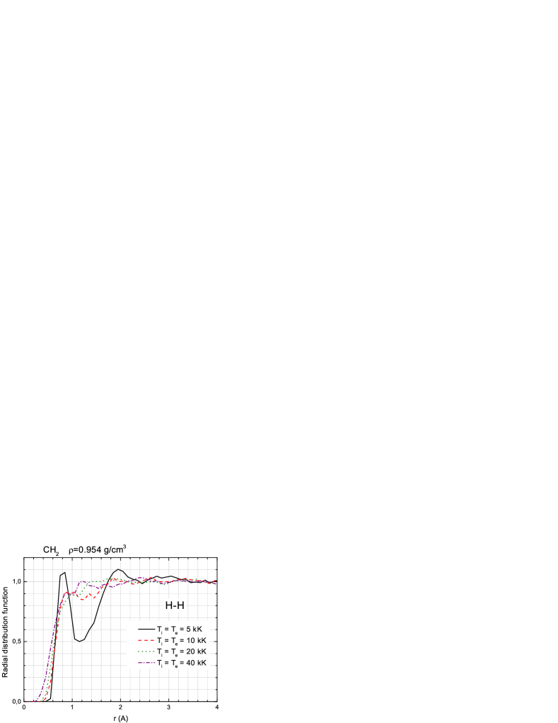
Figure 3: Same as Fig. 1 but for H-H radial distribution functions.

It is convenient to start the discussion of the results from the RDFs. The general view in Figs. 1–3 shows, that there are peaks at the RDF curves at low temperatures; these peaks vanish at higher temperatures. In the further discussion we will assume that these peaks are due to the chemical bonds.

Strictly speaking, the presence of chemical bonds may not be reliably established based on the analysis of RDFs only. The peaks at RDF curves have only the following meaning: the interionic distances possess in average certain values $\{r_{\mathrm{peak}}\}$ more often than other values. But nothing may be said about how long the ions are located at these $\{r_{\mathrm{peak}}\}$ distances from each other. We should check that ions are located at $\{r_{\mathrm{peak}}\}$ for certain periods of time $\{t_{\mathrm{peak}}\}$; only in this case we may establish reliably the presence of chemical bonds. These periods $\{t_{\mathrm{peak}}\}$ may be called the lifetimes of chemical bonds. This complicated analysis may be found in the papers Mattsson et al. (2010); Magyar et al. (2015). However, in the current work we will use only RDFs to register chemical bonds.

Fig. 1(a), Fig. 2(a), Fig. 3(a) show the RDFs at fixed $T_{i}=5$ kK and various $T_{e}$ from 5 kK up to 40 kK. If $T_{e}$ increases from 5 kK to 10 kK, the bonds are almost intact and the RDF curves almost do not change (only H-H bonds decay to some extent). At $T_{e}=20$ kK C-C and C-H bonds are mostly intact (though the peaks become lower); only H-H bonds break almost totally. And only if $T_{e}$ is risen to 40 kK all the bonds decay.

The situation is different in the one-temperature case $T_{i}=T_{e}=T$ (Fig. 1(b), Fig. 2(b), Fig. 3(b)). The increase of $T$ from 5 kK to 10 kK already makes the bonds decay. Given the influence of $T_{e}$ on the bonds is rather weak in this temperature range (see above), this breakdown of bonds is totally due to the increase of $T_{i}$. At $T=10$ kK H-H bonds are already destroyed totally (Fig. 3(b)), C-H bonds—almost totally (Fig. 2(b)), C-C bonds—considerably (Fig. 1(b)). The increase of $T$ to 20 kK leads to the almost complete decay of all bonds.

The following conclusions may be derived from the performed consideration of the RDF curves. If $T_{i}$ is kept rather low (5 kK), $T_{e}$ should be risen to 20 kK–40 kK to destroy the bonds. If both $T_{e}$ and $T_{i}$ are increased simultaneously (and $T_{e}=T_{i}$), temperatures 10 kK–20 kK are quite enough to break the bonds.

The temperature dependences of $[\mathcal{E}-\mathcal{E}_{i}^{\mathrm{kin}}]$ and $\sigma_{1_{\mathrm{DC}}}$ are presented in Figs. 4–5. The behavior of the calculated properties depends largely on whether the bonds are destroyed or not.

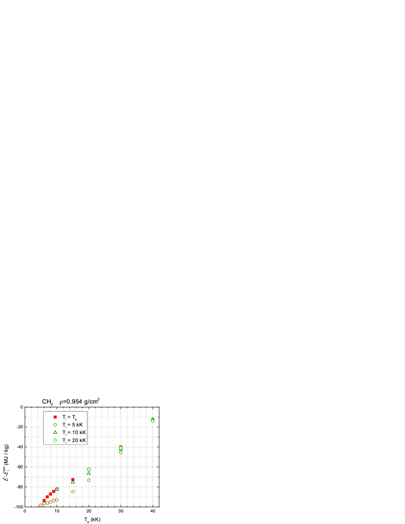
a)  b) 

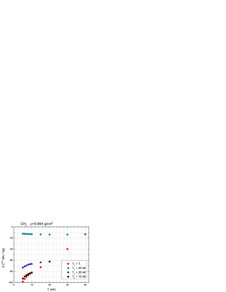
Figure 4: Specific energy without kinetic contribution of ions $[\mathcal{E}-\mathcal{E}_{i}^{\mathrm{kin}}]$ at different temperatures. (a) Dependence on the electron temperature $T_{e}$. Filled squares—one-temperature case $T_{i}=T_{e}$. Empty circles—fixed $T_{i}=5$ kK; empty triangles—fixed $T_{i}=10$ kK; empty diamonds—fixed $T_{i}=20$ kK. (b) Dependence on the ion temperature $T_{i}$. Filled squares—one-temperature case $T_{e}=T_{i}$. Filled circles—fixed $T_{e}=10$ kK; filled triangles—fixed $T_{e}=20$ kK; filled diamonds—fixed $T_{e}=40$ kK.

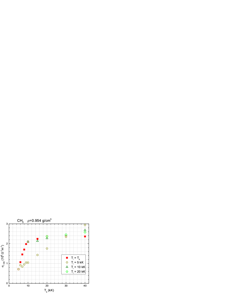
a)  b) 

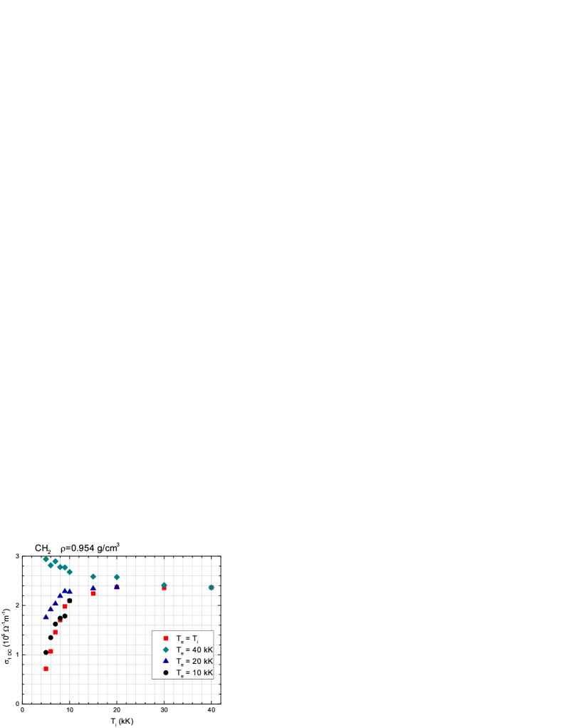
Figure 5: Same as Fig. 4, but for static electrical conductivity $\sigma_{1_{\mathrm{DC}}}$.

The obtained results may be divided into three characteristic cases.

1) 5 kK $\leq T_{i}\leq T_{e}\leq 10$ kK. The considerable number of bonds are present in the system under these conditions. The chemical bonds break rapidly as $T_{i}$ grows, and decay rather slowly as $T_{e}$ increases.

$[\mathcal{E}-\mathcal{E}_{i}^{\mathrm{kin}}]$ increases rapidly as $T_{i}$ grows (Fig. 4(b)), and increases slowly as $T_{e}$ grows (Fig. 4(a)). $\sigma_{1_{\mathrm{DC}}}$ increases rapidly as $T_{i}$ grows (Fig. 5(b)) and increases slowly as $T_{e}$ grows (Fig. 5(a)).

Thus the growth of $[\mathcal{E}-\mathcal{E}_{i}^{\mathrm{kin}}]$ and the growth of $\sigma_{1_{\mathrm{DC}}}$ correlate somewhat with the destruction of the chemical bonds: these processes occur rapidly if $T_{i}$ rises, and slowly with the rise of $T_{e}$.

In the one-temperature situation (5 kK $\leq T_{i}=T_{e}=T\leq 10$ kK) $[\mathcal{E}-\mathcal{E}_{i}^{\mathrm{kin}}](T)$ increases as $T$ grows, this increase is mostly determined by $T_{i}$ influence (i.e. by the second term in the right hand side of Eq. (1)). The $\left(\frac{\partial[\mathcal{E}-\mathcal{E}_{i}^{\mathrm{kin}}]}{\partial T_{i}}\right)_{T_{e}}$ contribution to $[\mathcal{C}_{v}-\mathcal{C}_{v\leavevmode\nobreak\ i}^{\mathrm{kin}}]$ is larger than $\left(\frac{\partial[\mathcal{E}-\mathcal{E}_{i}^{\mathrm{kin}}]}{\partial T_{e}}\right)_{T_{i}}$ (see Eq. (3) and Fig. 4). Since the growth of $[\mathcal{E}-\mathcal{E}_{i}^{\mathrm{kin}}]$ correlates with the destruction of bonds here, we may assume that the energy supply necessary for the bond decay gives the main contribution to $[\mathcal{C}_{v}-\mathcal{C}_{v\leavevmode\nobreak\ i}^{\mathrm{kin}}]$.

The rapid growth of $\sigma_{1_{\mathrm{DC}}}(T)$ in the one-temperature situation is mostly due to the influence of $T_{i}$.

2) 20 kK $\leq T_{i}\leq T_{e}\leq 40$ kK. There are no chemical bonds in the system under these conditions.

$[\mathcal{E}-\mathcal{E}_{i}^{\mathrm{kin}}]$ grows as $T_{e}$ increases (Fig. 4(a)) and is almost independent of $T_{i}$ (Fig. 4(b)). $[\mathcal{E}-\mathcal{E}_{i}^{\mathrm{kin}}]$ includes the kinetic energy of electrons, electron-electron, electron-ion and ion-ion potential energies. The fact, that $[\mathcal{E}-\mathcal{E}_{i}^{\mathrm{kin}}]$ does not depend on $T_{i}$, is intuitively clear: there are no significant changes of the ionic structure under the conditions considered (the decay of chemical bonds could be mentioned as a possible example of such changes).

$\sigma_{1_{\mathrm{DC}}}$ increases as $T_{e}$ grows (Fig. 5(a)) and decreases as $T_{i}$ grows (Fig. 5(b)).

In the one-temperature situation (20 kK $\leq T_{i}=T_{e}=T\leq 40$ kK) $[\mathcal{E}-\mathcal{E}_{i}^{\mathrm{kin}}](T)$ increases as $T$ grows only due to $T_{e}$ influence (i.e. due to the first term in the right hand side of Eq. (1)). $[\mathcal{C}_{v}-\mathcal{C}_{v\leavevmode\nobreak\ i}^{\mathrm{kin}}]$ totally equals $\left(\frac{\partial[\mathcal{E}-\mathcal{E}_{i}^{\mathrm{kin}}]}{\partial T_{e}}\right)_{T_{i}}$ here (Eq. (3)). We can assume that the temperature excitation of the electron subsystem determines $[\mathcal{C}_{v}-\mathcal{C}_{v\leavevmode\nobreak\ i}^{\mathrm{kin}}]$ values in this situation.

$\sigma_{1_{\mathrm{DC}}}$ decreases as $T_{i}$ grows and increases as $T_{e}$ grows. In the one-temperature case these two opposite effects compensate each other totally and form $\sigma_{1_{\mathrm{DC}}}(T)$, that does not depend on $T$.

3) 5 kK $\leq T_{i}\leq 10$ kK, 30 kK $\leq T_{e}\leq 40$ kK. This case is qualitatively close to the second one. There are no chemical bonds in the system.

$[\mathcal{E}-\mathcal{E}_{i}^{\mathrm{kin}}]$ increases as $T_{e}$ grows (Fig. 4(a)) and does not depend on $T_{i}$ (Fig. 4(b)); $\sigma_{1_{\mathrm{DC}}}$ increases as $T_{e}$ grows (Fig. 5(a)) and decreases as $T_{i}$ grows (Fig. 5(b)).

V Conclusion

In this paper we have calculated the properties of CH₂ plasma in the two-temperature case. First of all, the properties at $T_{e}>T_{i}$ are of significant interest for the simulation of rapid laser experiments. The performed calculations also help us to understand better the properties in the one-temperature case $T_{i}=T_{e}=T$. Two characteristic regions of the one-temperature curves Knyazev and Levashov (2015) may be considered.

The first region corresponds to the temperatures of 5 kK $\leq T\leq 10$ kK. The significant number of chemical bonds exist in the system in this case. These bonds decay if $T$ is increased (mainly because of heating of ions). We assume, that the energy necessary for the destruction of bonds gives the main contribution to $[\mathcal{C}_{v}-\mathcal{C}_{v\leavevmode\nobreak\ i}^{\mathrm{kin}}]$ in this region. The decay of bonds also correlates with the rapid growth of $\sigma_{1_{\mathrm{DC}}}$.

The second region corresponds to the temperatures of 20 kK $\leq T\leq 40$ kK. The system contains no chemical bonds under these conditions. The growth of $[\mathcal{E}-\mathcal{E}_{i}^{\mathrm{kin}}](T)$ is totally determined by heating of electrons. We assume, that the temperature excitation of the electron subsystem determines $[\mathcal{C}_{v}-\mathcal{C}_{v\leavevmode\nobreak\ i}^{\mathrm{kin}}]$ values here. $\sigma_{1_{\mathrm{DC}}}$ is influenced by heating of both electrons and ions moderately and oppositely. These opposite effects form the plateau on $\sigma_{1_{\mathrm{DC}}}(T)$ dependence in the second region.

References

- Povarnitsyn et al. (2013) M. E. Povarnitsyn, N. E. Andreev, P. R. Levashov, K. V. Khishchenko, D. A. Kim, V. G. Novikov, and O. N. Rosmej, Laser and Particle Beams 31, 663 (2013).
- Povarnitsyn et al. (2015) M. E. Povarnitsyn, V. B. Fokin, P. R. Levashov, and T. E. Itina, Phys. Rev. B 92, 174104 (2015).
- Ovechkin et al. (2014) A. A. Ovechkin, P. A. Loboda, V. G. Novikov, A. S. Grushin, and A. D. Solomyannaya, High Energy Density Physics 13, 20 (2014).
- Apfelbaum (2016) E. M. Apfelbaum, Contrib. Plasma Phys. 56, 176 (2016).
- Wang and Zhang (2013) C. Wang and P. Zhang, Phys. Plasmas 20, 092703 (2013).
- Wang et al. (2013) C. Wang, Y. Long, M.-F. Tian, X.-T. He, and P. Zhang, Phys. Rev. E 87, 043105 (2013).
- Minakov et al. (2014) D. V. Minakov, P. R. Levashov, K. V. Khishchenko, and V. E. Fortov, J. Appl. Phys. 115, 223512 (2014).
- Minakov and Levashov (2015) D. V. Minakov and P. R. Levashov, Phys. Rev. B 92, 224102 (2015).
- Desjarlais et al. (2002) M. P. Desjarlais, J. D. Kress, and L. A. Collins, Phys. Rev. E 66, 025401 (2002).
- Recoules and Crocombette (2005) V. Recoules and J.-P. Crocombette, Phys. Rev. B 72, 104202 (2005).
- Hu et al. (2015) S. X. Hu, V. N. Goncharov, T. R. Boehly, R. L. McCrory, S. Skupsky, L. A. Collins, J. D. Kress, and B. Militzer, Phys. Plasmas 22, 056304 (2015).
- Li et al. (2015) Ch.-Y. Li, C. Wang, Z.-Q. Wu, Z. Li, D.-F. Li, and P. Zhang, Phys. Plasmas 22, 092705 (2015).
- Norman et al. (2015) G. Norman, I. Saitov, V. Stegailov, and P. Zhilyaev, Phys. Rev. E 91, 023105 (2015).
- Migdal et al. (2016) K. P. Migdal, Yu. V. Petrov, D. K. Il’nitsky, V. V. Zhakhovsky, N. A. Inogamov, K. V. Khishchenko, D. V. Knyazev, and P. R. Levashov, Appl. Phys. A 122, 408 (2016).
- Mattsson et al. (2010) T. R. Mattsson, J. M. D. Lane, K. R. Cochrane, M. P. Desjarlais, A. P. Thompson, F. Pierce, and G. S. Grest, Phys. Rev. B 81, 054103 (2010).
- Wang et al. (2011) C. Wang, X.-T. He, and P. Zhang, Phys. Plasmas 18, 082707 (2011).
- Lambert and Recoules (2012) F. Lambert and V. Recoules, Phys. Rev. E 86, 026405 (2012).
- Hamel et al. (2012) S. Hamel, L. X. Benedict, P. M. Celliers, M. A. Barrios, T. R. Boehly, G. W. Collins, T. Döppner, J. H. Eggert, D. R. Farley, D. G. Hicks, J. L. Kline, A. Lazicki, S. LePape, A. J. Mackinnon, J. D. Moody, H. F. Robey, E. Schwegler, and P. A. Sterne, Phys. Rev. B 86, 094113 (2012).
- Chantawansri et al. (2012) T. L. Chantawansri, T. W. Sirk, E. F. C. Byrd, J. W. Andzelm, and B. M. Rice, J. Chem. Phys. 137, 204901 (2012).
- Hu et al. (2014) S. X. Hu, T. R. Boehly, and L. A. Collins, Phys. Rev. E 89, 063104 (2014).
- Danel and Kazandjian (2015) J.-F. Danel and L. Kazandjian, Phys. Rev. E 91, 013103 (2015).
- Horner et al. (2010) D. A. Horner, J. D. Kress, and L. A. Collins, Phys. Rev. B 81, 214301 (2010).
- Magyar et al. (2015) R. J. Magyar, S. Root, K. Cochrane, T. R. Mattsson, and D. G. Flicker, Phys. Rev. B 91, 134109 (2015).
- Huser et al. (2015) G. Huser, V. Recoules, N. Ozaki, T. Sano, Y. Sakawa, G. Salin, B. Albertazzi, K. Miyanishi, and R. Kodama, Phys. Rev. E 92, 063108 (2015).
- Colin-Lalu et al. (2015) P. Colin-Lalu, V. Recoules, G. Salin, and G. Huser, Phys. Rev. E 92, 053104 (2015).
- Knyazev and Levashov (2015) D. V. Knyazev and P. R. Levashov, Phys. Plasmas 22, 053303 (2015).
- Knyazev and Levashov (2013) D. V. Knyazev and P. R. Levashov, Comput. Mater. Sci. 79, 817 (2013).
- Knyazev and Levashov (2014) D. V. Knyazev and P. R. Levashov, Phys. Plasmas 21, 073302 (2014).
- Kresse and Hafner (1993) G. Kresse and J. Hafner, Phys. Rev. B 47, 558 (1993).
- Kresse and Hafner (1994) G. Kresse and J. Hafner, Phys. Rev. B 49, 14251 (1994).
- Kresse and Furthmüller (1996) G. Kresse and J. Furthmüller, Phys. Rev. B 54, 11169 (1996).
- Humphrey et al. (1996) W. Humphrey, A. Dalke, and K. Schulten, J. Mol. Graphics 14, 33 (1996).
- Perdew and Zunger (1981) J. P. Perdew and A. Zunger, Phys. Rev. B 23, 5048 (1981).
- Blöchl (1994) P. E. Blöchl, Phys. Rev. B 50, 17953 (1994).
- Kresse and Joubert (1999) G. Kresse and D. Joubert, Phys. Rev. B 59, 1758 (1999).