A stage-structured Bayesian hierarchical model for salmon lice populations at individual salmon farms - Estimated from multiple farm data sets

Abstract Salmon farming has become a prosperous international industry over the last decades. Along with growth in the production farmed salmon, however, an increasing threat by pathogens has emerged. Of special concern is the propagation and spread of the salmon louse, Lepeophtheirus salmonis. In order to gain insight into this parasites population dynamics in large scale salmon farming system, we present a fully mechanistic stage-structured population model for the salmon louse, also allowing for complexities involved in the hierarchical structure of full scale salmon farming. The model estimates parameters controlling a wide range of processes, including temperature dependent demographic rates, fish size and abundance effects on louse transmission rates, effects sizes of various salmon louse control measures, and distance based between farm transmission rates. Model parameters were estimated from data including 32 salmon farms, except the last production months for five farms which were used to evaluate model predictions. We used a Bayesian estimation approach, combining the prior distributions and the data likelihood into a joint posterior distribution for all model parameters. The model generated expected values that fitted the observed infection levels of the chalimus, adult female and other mobile stages of salmon lice, reasonably well. Predictions for the time periods not used for fitting the model were also consistent with the observational data. We argue that the present model for the population dynamics of the salmon louse in aquaculture farm systems may contribute to resolve the complexity of processes that drive that drive this host-parasite relationship, and hence may improve strategies to control the parasite in this production system.

KEY WORDS: population model, aquaculture, stochastic model, sea lice counts

1 Introduction

Salmon farming has become a large and economically prosperous international industry over the last decades. Norway holds a leading position as a producer of farmed salmonids with an annual production of about 1.2 million tonnes, which is roughly half of the worldwide production (Anonymous, 2015). Further growth in the production of salmonids is in demand (Anonymous, 2015) , but this will come at the cost of increasing risks of pathogen propagation and transmission. Large-scale host density dependence acting on pathogen transmission has been demonstrated in salmon farming production systems, both for macro parasites (Aldrin et al., 2013; Jansen et al., 2012; Kristoffersen et al., 2014) and viruses (Aldrin et al., 2011, 2010; Kristoffersen et al., 2009). Of special concern, is the propagation and spread of the salmon louse, Lepeophtheirus salmonis, and this parasite’s potentially harmful effect on wild salmon populations (Krkošek et al., 2007).

Mathematical and statistical models are increasingly being used to evaluate infection pathways and risk factors for pathogen propagation and disease development, both in aquatic and terrestrial animal farming (Aldrin et al., 2013, 2011, 2010; Salama and Murray, 2013; Murray and Salama, 2016; Jonkers et al., 2010; Diggle, 2006; Höhle, 2009; Keeling et al., 2001; Scheel et al., 2007). When such models are able to describe the main patterns in the host-pathogen population dynamics, including the spread within and between farms, they can be used to predict future infection levels as well as simulate the outcomes of disease mitigation scenarios, examples being interventions to mitigate bovine tuberculosis in Great Britain (Brooks-Pollock et al., 2014) and long term effects of infection control measurements to mitigate salmonid alphavirus (SAV) incidences causing pancreas disease (PD) outbreaks (Aldrin et al., 2015). The Norwegian salmonid production system is exceptionally well suited for developing models for salmon lice infection dynamics because of the wealth of surveillance time-series that document both the spatial locations and population sizes of host populations at risk of infection, as well as salmon lice abundances in these host populations. Coupling these host and parasite population data have provided insights into e.g. how salmon lice spread between farms depending on between-farm distances, and how transmission and parasite abundances depend on local host biomasses (Jansen et al., 2012; Aldrin et al., 2013; Kristoffersen et al., 2014). However, previous models that describe both between and within farm parasite population dynamics have for simplicity typically been autoregressive statistical models focusing on single aggregated measures of parasite infection levels (Jansen et al., 2012; Aldrin et al., 2013; Kristoffersen et al., 2013, 2014). Alternatively, models have been developed for simulation purposes only (Groner et al., 2014) or focused on the population dynamics on single farms over a limited time period (Krkošek et al., 2010). Most of these approaches have relied heavily on estimates of demographic rates obtained in the laboratory (Stien et al., 2005; Revie et al., 2005; Gettinby et al., 2011; Groner et al., 2013; Rittenhouse et al., 2016; Groner et al., 2016).

The aim of the present paper is to formulate a fully mechanistic stage-structured population model for the salmon louse, that also allows for the complexities involved in full scale salmon farming. Furthermore, the model accounts for the hierarchical structure of the data obtained from the production system where salmon lice are counted on subsamples of fish, the fish being aggregated into separate cages and the cages being aggregated to farm. The model estimates parameters controlling a wide range of processes, including effects of temperature on demographic rates, fish size and abundance effects on transmission rates, the different effect sizes, temporal and stage specific effects of a wide range of salmon lice control measures, and distance-based transmission rates between farms. The objectives for developing such a complex population model for the salmon louse are: 1) To evaluate whether estimates of demographic rates obtained in the laboratory seems applicable in full scale production settings. 2) To evaluate the efficiency of different control measures. 3) To explore importance of different sources of infection (e.g. internal versus external sources). 4) To develop a tool that can keep account of the salmon louse populations at the production unit level in salmon farms, based on the successive counting of salmon louse infestations. 5) To develop a tool for short term predictions of salmon louse infection levels. 6) Finally, to develop a sufficiently realistic model that can be used for scenario-simulations exploring the effects of various parasite control strategies. In this paper, we describe the model in detail and discuss the results in relation to objectives 1-5.

2 Materials and methods

2.1 Modelling background

Many authors have previously presented models for salmon louse population dynamics. Most of these models are formulated on a continuous time scale (Stien et al., 2005; Revie et al., 2005; Gettinby et al., 2011; Groner et al., 2013; Rittenhouse et al., 2016; Krkošek et al., 2009) , whereas others are formulated at a discrete scale with a time step one day (Groner et al., 2016), which is also the case for our model. However, more important when comparing with our model is that the parameter values in previous models primarily are based on laboratory data or on small scale experimental units in the marine environment. When real production data has been used for estimation, these have been aggregated. For instance, Stien et al. (2005) used only laboratory data published in previous papers, whereas Groner et al. (2013) and Groner et al. (2016) used values from Stien et al. (2005) for some parameters and values from several other previous papers for other parameters. Furthermore, Revie et al. (2005) and Gettinby et al. (2011) used laboratory data from previous studies to estimate the majority of the parameters and real production data to estimate the remaining parameters, but the production data were aggregated over farms and to a monthly time scale. One exception is the study by Krkošek et al. (2009), who estimated their model by experimental data from small scale marine cages, but their model covers only the parasitic stages of the salmon louse.

The present estimating approach is fundamentally different. The parameters are estimated by fitting the model to every lice count collected through the whole production period on each cage at each of 32 farms. However, to ensure that the final parameter values are within biological plausible ranges, we use laboratory data, mostly based on results summarised in Stien et al. (2005), to specify informative prior distributions for many of the parameters. The priors are then updated to posterior distributions by the full scale farm data using Bayesian methods. Since the model is estimated on real data from many different farms under various conditions, it has to simultaneously incorporate many features to handle activities or events that affect lice abundance, including various types of treatments, external infection from neighbouring farms and the movement of fish (and then also lice) between cages at the same farm. Our model is therefore more complex than the aforementioned models.

For instance, our model takes into account and estimate the effect of several different types of treatments, such as medical bath treatments, in-feed treatments and the use of cleaner fish. Of the aforementioned models, the model of Groner et al. (2013) includes the effect of cleaner fish, but the effect size was taken from previous studies from the 1990-ies. Likewise, the models used in Revie et al. (2005), Gettinby et al. (2011) and Groner et al. (2013) include effects of medical treatments, but again the values of the effects were based on previous studies. Our model is designed to allow new interventions to be incorporated and their effect on lice abundances to be estimated from real-time production data.

Fish are always free of lice when they are stocked as smolt to seawater cages, so the lice population at a farm is always initiated by external infection. The models used in Revie et al. (2005), Gettinby et al. (2011) and Groner et al. (2013) include external infection as a constant, estimated from aggregated data. In our model, the external infection is farm-specific and time-varying, depending on abundance of adult female lice at neighbouring farms. Because we intend to maximise the model fit to each lice count at each cage at each farm, some of the parameters in our model are farm-specific or even cage-specific and some are time-varying, whereas other parameters are constant and common for all cages and farms.

2.2 Salmon farming and salmon lice

Farm production of salmon comprises of a freshwater juvenile phase, being followed by a marine grow out phase, the latter which is the focus of this study. The production of salmon on a marine farm typically initiates by stocking juvenile smolts to cages (or net-pens) either in spring or in autumn. Salmon are kept in the marine farms for about 1.5 years after which they are slaughtered for food consumption. In Norway, only fish of the same year class of age are kept on a given farm and we term this a cohort throughout the present paper. After slaughtering, it is mandatory to fallow the farm for a period of at least two months before stocking a new cohort of salmon. Fish may occasionally be moved from one marine farm location to an empty farm location, in which case this farm will initially report fish weights larger than expected for smolts recently stocked into the sea.

2.3 Data

The main body of data in the present study consist of cage-level data from 32 marine salmon farms in Norway, of which 12 farms are located north of the island Frøya in Mid-Norway (Figure 1). For each farm, the data covers a full production cycle for farmed salmon, from stocking as smolts to slaughtering as adult Atlantic salmon (Salmo salar L.), including fish production data, lice counts, temperatures and louse control efforts. Salmon were stocked between 2011 and 2013 and slaughtered about 1 1/2 year after stocking, between 2012 and 2014. The number of production units (cages) per farm varied from 3 to 12, but were usually around 8 (mean 7.7). For 9 farms, the fish were moved between cages within the farm during the production period.

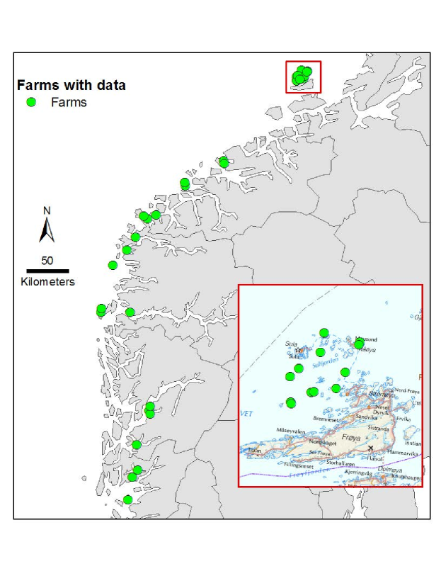
Figure 1: Geographical positions of the 32 salmon farms on the West coast of Norway (green circles). The highlighted area contains the 12 farms in Nord-Frøya.

Seawater temperatures were measured at 5 m depth at the farms. The average temperature was 9.1^∘C, and 95 % of the temperatures were between 3.6 and 15.0^∘C. Data on salinity were not available in sufficient detail and have therefore not been used.

The production data consist of daily numbers and mean weights of salmon per cage during the production period, information on movement of salmon between cages within farms and information on antiparasitic lice treatment using chemotherapeutic medicals (day of application and type of medical). Furthermore, the data contain information on stocking of cleaner fish (day and number of cleaner fish stocked), but with limited information on their mortality, and hence also for the number of cleaner fish present at a given day. We do not distinguish between various species of cleaner fish.

The production cycles lasted on average 16.5 months per cage, with on average 140 000 fish per cage, typically more in the beginning of a production cycle and less towards the end. The average minimum and maximum fish weights during a production cycle was 140 g and 5.7 kg, respectively. 89 % of the cages contained cleaner fish in parts of the production period.

As a main rule, lice counts were performed on a sample of at least 10 fish every second week for each cage. The salmon lice were divided into three categories according to developmental stages, i.e. i) chalimus (CH), ii) other mobiles (OM), which consist of pre-adults and adult males, and iii) adult females (AF). There were on average 41 lice counts per cage, with averages (abundance) of 0.23 CH, 0.76 OM and 0.18 AF per fish.

Six different types of antiparasitic medicals were used (Table 1), and there were on average 4.6 events of medical treatments per cage. We assume that the effects of deltamethrin and cypermethrin are equal, since these are similar compounds. Furthermore, when azamethiphos is used in combination with deltamethrin or cypermethrin, we assume it has the same effect as using deltamethrin or cypermethrin alone, since this combination is used when reduced treatment effect is expected due to resistance towards the medicals. The medicals emamectin benzoate and diflubenzuron are given through the feed, typically over a period of around two weeks. These treatments have a relatively low daily effect, but effects last over a prolonged period. The other medicals are applied as bath treatments over a duration of a few hours, with a larger daily effect, but lasting over a shorter period. We assume it is a time delay of $\Delta^{del}$ days (Table 1) after application before the treatments give visible effects. Furthermore, we assume that the duration of the effect, $\Delta^{dur}$, depends on the seawater temperature according to

$$\Delta^{dur} = \delta^{dur}/T_{t^{0}},$$ (1)

where $\delta^{dur}$ is a constant given in Table 1 and $T_{t^{0}}$ is the seawater temperature when the medical is applied. One exception is when hydrogen peroxide was applied, for which $\Delta^{dur}$ is temperature independent and given by $\Delta^{dur}=\delta^{dur}$ (in days).

Table 1: Overview of types of medical treatments used. Codes: Y=yes, N=no, NA=missing information. The table content is based on information in Nygaard (2010) and Ottesen et al. (2012). For hydrogen peroxide, the unit for $\delta^{dur}$ is days.

			Duration
		Delay	constant
	Product	$\Delta^{del}$	$\delta^{dur}$	Temperature	Effect	Effect	Effect	Effect
Medical	name	(days)	(days $\cdot^{\circ}\mathrm{C}$)	dependency	on CH	on PA	on A	on egg
Deltamethrin	Alphamax	2	84	Y	Y	Y	Y	N
Cypermethrin	Betamax	2	84	Y	Y	Y	Y	N
Azamethiphos	Salmosan	1	42	Y	N	Y	Y	N
Hydrogen peroxide (H2O2)		0	7	N	N	Y	Y	NA
Emamectin benzoate	Slice	5	210	Y	Y	Y	Y	NA
Diflubenzuron	Releeze	10	126	Y	Y	Y	N	N

In addition to the detailed cage-level data on the 32 farms, we have more aggregated data on all other Norwegian marine salmon farms. For a farm $f^{\prime}$ at day $t$, we know the number of salmon, denoted by $N_{tf^{\prime}}^{SAL}$. We also have an estimate $\widehat{A}^{AF}_{tf^{\prime}}$ of the abundance of AF lice at the farm, based on weekly lice counts on a sample of fish, and therefore also an estimate of the total number of AF lice, given by $\widehat{N}^{AF}_{tf^{\prime}}=\widehat{A}^{AF}_{tf^{\prime}}N_{tf^{\prime}}^{SAL}$. Finally, we have the seaway distances between all farms, and we let $d_{ff^{\prime}}$ denote the seaway distance between a farm $f$ and another farm $f^{\prime}$.

Based on these quantities for all other farms, we have calculated an external infection pressure index for each of the 32 farms, which can be seen as a preliminary estimate of external infection pressure at time $t$. This is a weighted sum of the estimated numbers of AF lice at neighbouring farms, where the weights decrease by increasing seaway distance to the farm in question. This index is denoted by $N_{tf}^{AFExt}$ for farm $f$ at time $t$, and is given by

$$N_{tf}^{AFExt} = \sum_{f^{\prime}\neq f}g(d_{ff^{\prime}})\widehat{N}^{AF}_{tf^{\prime}},$$ (2)

where $g(\cdot)$ is a function decreasing by increasing distance given by

$$g(d) = \exp(-0.618d^{0.568}).$$ (3)

This distance function is taken from Aldrin et al. (2013), and is based on a data-driven model for lice abundance estimated from more than eight years of data on all 1400 Norwegian salmon farms that were active in the data period.

We have also calculated a corresponding weighted average of the counted abundance of adult females at neighbouring farms, given by

$$A_{tf}^{AFExt} = \sum_{f^{\prime}\neq f}g(d_{ff^{\prime}})\widehat{A}^{AF}_{tf^{\prime}}/\sum_{f^{\prime}\neq f}g(d_{ff^{\prime}}),$$ (4)

Figure 2 shows the most relevant data for one cage at one farm. The upper panel shows time plots of the seawater temperature (on the left y-axis) and the external infection pressure index. In addition, the first stocking of salmon in this cage is indicated by the vertical pink line and the various medical treatments are shown as blue vertical lines. Finally, the stocking of cleaner fish is also shown as vertical lines. The vertical extension of these lines is proportional to the stocked cleaner fish ratio (on the right y-axis), i.e. the number of stocked cleaner fish divided by the number of salmon. The lower three panels show the counted abundance of lice in the CH, OM and AF categories.

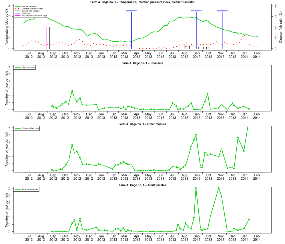
Figure 2: Counted lice abundance and other information for one cage at one farm. Upper panel: Seawater temperature (green line), external infection pressure index (red dotted curve), time of stocking (pink vertical line), treatments (blue vertical lines) and stocked cleaner fish ratio (black vertical lines). Three lower panels: Counts of chalimi, other mobiles or adult females shown as green circles connected by straight lines.

2.4 Model framework

2.4.1 Some model overview and notation

Biologically, the life cycle of the salmon louse consists of eight developmental stages (Hamre et al., 2013). These are aggregated into the following five stages in our model: i) recruits (R, eggs and nauplii larvae), ii) copepodids (CO, infective planktonic larvae), iii) chalimi (CH, sessile lice on fish), iv) pre-adults (PA, mobile lice on fish) and v) adults (A, also mobile lice on fish). The adults are further divided into adult females (AF) and adult males (AM). When an infective copepodid (stage CO) attaches to a fish host, it takes approximately 24 hours before it moults into the CH stage (Krkošek et al., 2009). We ignore this short period and assume that a copepodid enters the CH stage immediately upon attachment to a fish host. The salmon lice count data from fish farms pool the stages PA and AM together in one category (OM), whereas the stages CH and AF are counted as separate categories.

The time resolution of the model is one day. The general idea is that for stage-age $a=0$, the lice have developed into the given stage from the previous stage, and that for $a>0$, the lice can develop into the subsequent stage. We further assume that within a day, in the following order;

• lice may be counted on a sample of fish,

• lice may die due to natural mortality or treatment,

• the surviving lice might develop to the next stage, and finally,

• fish, with sessile or mobile lice, can be moved to another cage or be slaughtered.

When fish are stocked to marine farms as smolt, they are free of lice, and hence the initial lice transmission is caused by external infections. Not until some lice at the farm have developed into adults, the internal infection process can start. The population model for a farm with two cages is illustrated by Figure 3. In the R and CO stages, the lice are associated with the farm, but not with any specific cage. From the CH stage and onwards, however, the lice infect fish and are therefore associated with specific cages. In the following subsections we describe the various aspects of the population model and how the model is related to lice count data. Table 2 gives an overview of the main notation we use.

The main elements of the model are inspired by the model in Stien et al. (2005), but with some extensions, e.g. to capture management interventions on the farms. The model is validated rather informally, by assessing whether parameter estimates are plausible and by graphical evaluation of predictions ahead in time for five farms where the last 3-11 months of data were not used in the estimation process.

The model is estimated from the available data by a Bayesian approach. We thus need prior distributions for the model parameters. Many of these priors are informative, based on results from laboratory experiments, e.g those reported in Stien et al. (2005). For some priors, however, we use more vague settings (see Section 2 in the Supplementary material for details).

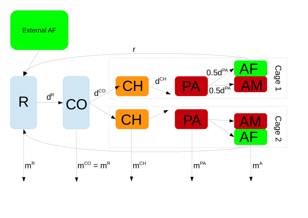
Figure 3: Overview of the population model for the salmon louse. Lice in the orange, red and green stages are counted, whereas lice in the blue stages are not counted. Lice are associated with a cage from the chalimus stage, here illustrated by a farm with two cages. The d-s, m-s and r-s symbolise development, mortality and recruitment, respectively.

Table 2: Overview of the model notation. When relevant, quantities may be used with subscripts $f$, $t$, $a$ and $c$, and with superscripts $R$, $CO$, $CH$, $PA$, $AF$ or $AM$

$f$	index for farm
$t$	index for time (day)
$a$	index for stage-age
$c$	index for cage
$N^{R}$	total number of lice recruits
$N^{CO}$	total number of copepodids
$N^{CH}$	total number of chalimus larvae on fish in a given cage
$N^{PA}$	total number of pre-adult lice on fish in a given cage
$N^{AF}$	total number of adult female lice on fish in a given cage
$N^{AM}$	total number of adult male lice on fish in a given cage
$s$	survival rate (proportion per day)
$m$	mortality rate ($m=1-s$)
$d$	development rate (proportion per day)
$r$	reproduction rate (numbers per day and per AF lice)
$N^{SAL}$	number of salmon
$W$	average weight of salmon
$M_{c^{\prime}c}^{SAL}$	number of salmon moved from cage $c^{\prime}$ to cage $c$
$w_{c^{\prime}c}$	proportion of salmon moved, $M_{c^{\prime}c}^{SAL}/N_{c^{\prime}}^{SAL}$
$N^{CLF}$	number of cleaner fish
$S^{CLF}$	number of cleaner fish stocked
$Y$	Number of lice counted on a sample of $n$ fish
$\lambda$	parameters related to mortality
$\delta$	parameters related to development
$\mu$	expected values
$\beta$, $\gamma$, $\kappa$, $\rho$	various parameters
$\sigma^{2}$	variances
$z$	autoregressive processes
$\phi$	autoregressive coefficients

2.4.2 Population model

Below, we present the population model for lice at a given farm (but for simplicity without the farm index $f$). The model consists of two equations per stage. The first equation handles lice entering a given stage at stage-age 0, typically from the preceding stage. The exception being the R stage, where the new recruits are the result of reproduction from adult females within the same farm and from neighbouring farms. The second per-stage equation handles lice ageing into higher stage-ages without developing into another stage.

The submodels for survival, development and reproduction rates are presented later in Sections 2.4.3, 2.4.4, 2.4.5 and 2.4.6.

Model for the recruitment stage

At the R stage, lice are not associated with a specific cage, but rather seen as a reservoir of recruits with the potential to infect a fish host at the farm in question in the future. The model is:

$$N_{t(a=0)}^{R} = e_{t}^{Ext}N_{t-1}^{AFExt}r^{Ext}_{t-1}+\sum_{c}\sum_{a^{\prime}}[N_{(t-1)a^{\prime}c}^{AF}s_{(t-1)a^{\prime}c}^{AF}r_{(t-1)a^{\prime}c}],$$ (5)

$$N_{t(a>0)}^{R} = N_{(t-1)(a-1)}^{R}s_{(t-1)(a-1)}^{R}[1-d_{(t-1)(a-1)}^{R}].$$ (6)

The first term in (5) represents recruitment (into stage-age 0) from neighbouring farms, also called external recruitment. Here, $N_{t-1}^{AFExt}$ is a weighted sum of adult females at neighbouring farms at time $t-1$ (see Section 2.3). Furthermore, we assume that these reproduce with a rate $r^{Ext}_{t-1}$ (see Section 2.4.7 ). Then, $N_{t-1}^{AFExt}r^{Ext}_{(t-1)}$ can be interpreted as a preliminary estimate of the number of external recruits reaching the farm. However, this accounts for seaway distances to neighbouring farms, but not for the sea currents in the area that may be more or less favourable for a given farm, and which also may vary over time. Therefore we have introduced the modifying factor $e_{t}^{Ext}$, which is a farm-dependent and time varying modifying factor, see Section 2.5 for an exact definition.

The second term in (5) represents recruitment (into stage-age 0) from adult female lice at the same farm, also called internal recruitment. The product $N_{(t-1)a^{\prime}c}^{AF}s_{(t-1)a^{\prime}c}^{AF}$ is the number of adult females at stage-age $a^{\prime}$ in cage $c$ that survives at time $t-1$ and they reproduce with a rate $r_{(t-1)a^{\prime}c}$ (see Section 2.4.6). The new recruits are summed over all possible stage-ages of the adult females and over all cages.

Eq. (6) keeps track of the number of recruits of stage-age $a>0$ that i) survives from the previous time point with survival rate $s_{(t-1)(a-1)}^{R}$ (see Section 2.4.3) and ii) do not develop into the infective CO stage, where $d_{(t-1)(a-1)}^{R}$ is the development rate, i.e. the proportion of recruits that develop into the CO stage (see Section 2.4.4).

The equations for the next stages use similar notation for survival rates, development rates and numbers of lice.

Model for the copepodid stage

$$N_{t(a=0)}^{CO} = \sum_{a^{\prime}}N_{(t-1)a^{\prime}}^{R}s_{(t-1)a^{\prime}}^{R}d_{(t-1)a^{\prime}}^{R},$$ (7)

$$N_{t(a>0)}^{CO} = N_{(t-1)(a-1)}^{CO}s_{(t-1)(a-1)}^{CO}[1-\sum_{c}d_{(t-1)(a-1)c}^{CO}].$$ (8)

Here, the development rate $d_{(t-1)(a-1)c}^{CO}$ (see Section 2.4.5) represents the infection rate, i.e. the proportion of the available copepodids that during a day infect fish in cage $c$ and thus enter the CH stage. The sum over cages, $d_{(t-1)(a-1)}^{CO}=\sum_{c}d_{(t-1)(a-1)c}^{CO}$ is then the total infection rate at the farm. This is modelled as independent of stage-age.

Model for the chalimus stage

$$N_{t(a=0)c}^{CH} = \sum_{a^{\prime}}N_{(t-1)a^{\prime}}^{CO}s_{(t-1)a^{\prime}}^{CO}d_{(t-1)a^{\prime}c}^{CO},$$ (9)

$$N_{t(a>0)c}^{CH} = \sum_{c^{\prime}}N_{(t-1)(a-1)c^{\prime}}^{CH}s_{(t-1)(a-1)c^{\prime}}^{CH}[1-d_{(t-1)(a-1)}^{CH}].$$ (10)

From the CH stage on, the lice are attached to a fish, and therefore associated with a specific cage. We assume that the attached lice follow the fish if the fish are moved to another cage or if the fish are removed from the farm (including slaughtering and other fish mortality). To handle this, the equations given here for the CH, PA and AF stages are extended slightly (see Section 1.2 in the Supplementary material).

Model for the pre-adult stage

$$N_{t(a=0)c}^{PA} = \sum_{a^{\prime}}\sum_{c^{\prime}}N_{(t-1)a^{\prime}c^{\prime}}^{CH}s_{(t-1)a^{\prime}c^{\prime}}^{CH}d_{(t-1)a^{\prime}}^{CH},$$ (11)

$$N_{t(a>0)c}^{PA} = \sum_{c^{\prime}}N_{(t-1)(a-1)c^{\prime}}^{PA}s_{(t-1)(a-1)c^{\prime}}^{PA}[1-d_{(t-1)(a-1)}^{PA}].$$ (12)

Model for the adult stages

For the adult stage, we distinguish in principle between males and females. However, we assume that males and females have the same survival and development rates and therefore each constitute 50 % of the adults. The main reason for this is that we do not have data on the number of adult males on the fish, and therefore do not have the information necessary for separate estimation of adult male demographic rates.. The equations for adult females are then

$$N_{t(a=0)c}^{AF} = 0.5\sum_{a^{\prime}}N_{(t-1)a^{\prime}c^{\prime}}^{PA}s_{(t-1)a^{\prime}c^{\prime}}^{PA}d_{(t-1)a^{\prime}}^{PA},$$ (13)

$$N_{t(a>0)c}^{AF} = \sum_{c^{\prime}}N_{(t-1)(a-1)c^{\prime}}^{AF}s_{(t-1)(a-1)c^{\prime}}^{AF},$$ (14)

while the number of adult males is equal to the number of adult females:

$$N_{tac}^{AM} = N_{tac}^{AF}.$$ (15)

2.4.3 Survival rates

We assume that the survival rates may be farm-specific for some stages, and therefore use the index $f$ when convenient, but we sometimes drop the superscript that indicates the stage name. We assume that the total survival rate is the product of three terms;

$$s_{tfac} = s_{tfac}^{nat}\cdot s_{tfac}^{clf}\cdot s_{tfac}^{cht}=(1-m_{tfac}^{nat})\cdot(1-m_{tfac}^{clf})\cdot(1-m_{tfac}^{cht}),$$ (16)

where $s_{tfac}^{nat}$ is survival after natural mortality, $s_{tfc}^{clf}$ is survival after additional mortality due to cleaner fish predation (independent of stage-age) and $s_{tfc}^{cht}$ is survival after additional mortality due to chemotherapeutic treatment (independent of stage-age). The $m$-s denote the corresponding mortalities. The two latter terms are relevant only for the CH, PA and A stages. All the three mortality (and survival) terms must lie between 0 and 1, but they have different structures.

Natural mortality

For the R and CO stages, we simply assume that the natural mortality is a constant that is common for both stages, i.e.

$$m_{tfac}^{Rnat} = m^{Rnat}=\lambda^{RCOnat},$$ (17)

$$m_{tfac}^{COnat} = m^{COnat}=\lambda^{RCOnat}$$ (18)

For each of the CH, PA and A stages, we assume that the natural mortalities are stochastic processes that can vary over time and between farms, but are common for all cages within a farm and independent of stage-age. This may account for factors that differ between farms and change over time, for instance salinity, which is not included in the model. Furthermore, including these mortalities as farm-specific and time-varying terms improves the fit of the model to data. For each farm and louse stage, the mortality is assumed to follow an autoregressive model of order 1 (AR(1)) on the logit-scale as

$$m_{tfac}^{nat} = m_{tf}^{nat}=\exp(z_{tf}^{nat}/(1+\exp(z_{tf}^{nat})),$$ (19)

$$(z_{tf}^{nat}-\lambda_{0}^{nat}) = \phi^{nat}\cdot(z_{(t-1)f}^{nat}-\lambda_{0}^{nat})+\varepsilon^{nat}_{tf},$$ (20)

$$\mathrm{Var}(\varepsilon^{nat}_{tf}) = (\sigma^{nat})^{2}.$$ (21)

Here, $z_{tf}^{nat}=\mbox{logit}(m_{tf}^{nat})=\log(m_{tf}^{nat}/(1-m_{tf}^{nat}))$. Furthermore, $\lambda_{0}^{nat}$ is the expected value on the logit-scale, $\phi^{nat}$ an autoregressive coefficient and $\varepsilon^{nat}_{tf}$ a white noise process with variance $(\sigma^{nat})^{2}$. These parameters have separate values for each stage. In addition, the time-varying mortalities $m_{tfac}^{nat}$ are restricted to lie within specified intervals, which are (0.0006-0.02) for CH, (0.002-0.21) for PA and (0.0003-0.70) for A. These limits are motivated from the various studies summarised in Stien et al. (2005), and are simply the most extreme limits of the intervals given in their Table 4.

In addition, we assume $m$ = 1 from stage-age 80 for adults and from stage-age 60 for the other stages. This is an approximation made to save computer time.

Mortality due to cleaner fish

We assume that cleaner fish feed on lice at the PA and A stages only (Leclercq et al., 2014), and that the corresponding mortality for these two stages are equal. Let $x_{tfc}^{clf}=N_{tfc}^{CLF}/N_{tfc}^{SAL}$ be the ratio of the number of cleaner fish to the number of salmon in cage $c$, at farm $f$ and time $t$. This ratio depends among others on the mortality of cleaner fish, which has to be estimated, and the model for this is described later in Section 2.5.1. Lice mortality in the PA and A stages due to cleaner fish is then given by

$$m_{tfac}^{clf} = m_{tfc}^{clf}=1-\exp(-\lambda^{clf}x_{tfc}^{clf}),$$ (22)

where the parameter $\lambda^{clf}$ is non-negative, such that the mortality always is between 0 and 1. One reason for assuming such a simple model for the effect of cleaner fish (as opposed to the effect of medical treatments discussed below) is that we also must estimate the cleaner fish ratio which is multiplied by the cleaner fish effect.

Mortality due to chemotherapeutic treatment

We assume that the chemotherapeutic treatments introduce extra mortality of lice in some or all the stages CH, PA and A, depending on the type of treatment. However, for simplicity we assume that lice are only affected as long as they stay in the stage they were at the time of treatment. If they manage to develop to the next stage, they are clear of the treatment effect. Let the set of subscripts $fcbi$ denote the $i$-th application of a chemotherapeutic of type $b$ in cage $c$ at farm $f$. Assuming that this treatment was given at time $t_{fcbi}^{0}$, we define an indicator variable $x_{tfacbi}^{cht}$ that is 1 when the treatment is active (a period after the treatment is given) for lice at stage-age $a$, i.e. when

$$t\in[t_{fcbi}^{0}+\Delta_{b}^{del},t_{fcbi}^{0}+\Delta_{b}^{del}+\Delta_{fcbi}^{dur})-1]\mbox{ and }a\geq t-t_{fcbi}^{0},$$ (23)

where the delay constant $\Delta_{b}^{del}$ and the duration $\Delta_{fcbi}^{dur}$ are explained in Section 2.3.

The mortality due to chemotherapeutic treatment is given by

$$m_{tfac}^{cht} = 1-\exp(\sum_{b}-u_{fcbi}^{cht}x_{tfacbi}^{cht}),$$ (24)

where $u_{fcbi}^{cht}$ is a regression coefficient expressing the effect of the specific application of the treatment. These regression coefficients vary systematically between treatment types, accounting for varying efficiency of different types of treatments. In addition, they vary randomly between different applications of the same treatment type, which for instance may be due to a varying degree of resistance in the lice populations. This is handled by the following formulation

$$u_{fcbi}^{cht} = \log(1+\exp(u_{fcbi}^{cht*})),$$ (25)

$$u_{fcbi}^{cht*} \sim \mathrm{N}(\lambda^{cht},(\sigma^{cht})^{2}).$$ (26)

In general, the parameters $\lambda^{cht}$ and $\sigma^{cht}$ differ between various types of treatment, but are set equal for some treatment types. These parameters are equal for the stages for which a treatment have effect, but the effect of a specific treatment $fcbi$, represented by the random coefficient $u_{fcbi}^{cht}$, may vary between stages (this is for simplicity omitted from the notation above).

2.4.4 Development rates

We consider here the development rate from one stage to the next, for the stages R, CH and PA. In all of the population models for lice that we mentioned in the introduction, the development rate is 0 until some, perhaps temperature-specific, minimum stage-age, and afterwards positive and constant. In our opinion, the concept of a strict and absolute minimum development time can be questioned in a population with millions of individuals, and the assumption of a constant development thereafter may be unrealistic. We have chosen to consider the development to the next stage as a time-to-event process, and model it as a discretised version of a Weibull distribution. The Weibull distribution is widely used in statistical models for time-to-event or survival analysis (Aalen et al., 2008). It also gave a better fit to our data than a comparable formulation that included the minimum development time model mentioned above as a special case (data not shown).

When the time to an event is continiuous and Weibull distributed, the event rate (often called hazard in survival analysis) is $(\delta^{sc})^{-\delta^{s}}\delta^{s}a^{\delta^{s}-1}$, where $a$ is the stage-age or time, $\delta^{s}$ is a shape parameter and $\delta^{sc}$ is a scale parameter (sometimes $(\delta^{sc})^{-\delta^{s}}$ is termed the scale parameter). In our case, it is convenient to re-parameterise this as a function of the median time to event, $\delta^{m}$, and the shape parameter. The event rate then becomes $\log(2)(\delta^{m})^{-\delta^{s}}\delta^{s}a^{\delta^{s}-1}$, since the median in the Weibull distribution is $\delta^{sc}(\log(2))^{(1/\delta^{s})}$.

We use a discretised version of this, i.e. our development rate is the probability to develop to the next stage within a day, and it must therefore also be restricted to be at most one. We assume that the median time to develop may vary over time and between farms, and introduce therefore the subscripts $tfa$ on it. The model for the development rate is then

$$d_{tfa} = \min(\log(2)(\delta_{tfa}^{m})^{-\delta^{s}}\delta^{s}a^{\delta^{s}-1},1)\quad\textrm{for}\quad a=0,1,\ldots\quad.$$ (27)

We further assume that the median development time depends on the temperature history as $\delta_{tfa}^{m}=c/(\bar{T}_{tfa})^{\delta^{p}}$, where $\bar{T}_{tfa}$ is the average temperature that lice at stage-age $a$ at farm $f$ have experienced, i.e. the average temperature from time $t-a$ to time $t$, $c$ is a constant and $\delta^{p}$ is another constant that performs a power transformation of $\bar{T}_{tfa}$. To get a more clear interpretation of the constant $c$, we parametrise it as a function of the median development time at 10^∘ C, denoted by $\delta^{m10}$. The final model for the median development time then becomes

$$\delta_{tfa}^{m} = (10^{\delta^{p}}\delta^{m10})/(\bar{T}_{tfa})^{\delta^{p}}=\delta^{m10}(10/\bar{T}_{tfa})^{\delta^{p}}.$$ (28)

The development rate defined by Eqs. (27) and (28) also depends on the stage in the way that the parameters $\delta^{m10}$, $\delta^{s}$ and $\delta^{p}$ are stage-specific. One motivation for introducing $\delta^{m10}$ as a basic parameter is that we use results on development times around 10^∘ C from other studies as prior information, to ensure that our estimates lies within biological plausible ranges. For the R stage, which consists of eggs and nauplii, this prior information is given separate for eggs and nauplii. Therefore, for the R stage, $\delta^{Rm10}$ is the sum of one parameter $\delta^{Em10}$ for eggs and another quantity $\delta^{Nm10}$ for nauplii, i.e.

$$\delta^{Rm10} =\delta^{Em10}+\delta^{Nm10}$$ , (29)

and $\delta^{Em10}$ is also contained in the reproduction factor introduced later in Section 2.4.6.

In the estimation, we restrict $\delta^{s}$ to be larger than 1, and the development rate will then be 0 at stage-age 0 and then increase by increasing stage-age. Furthermore, the larger $\delta^{s}$ is, the more steep will the development rate increase from 0 to 1 around the median. When $\delta^{s}>2$, the difference between the mean and the median will be less than 7 %. It should further be noted that the parameter $\delta^{m10}$ is only approximately the median development time, since we consider a time-discrete version of the Weibull distribution.

Assuming a constant temperature $T$, Stien et al. (2005) modelled the minimum development time as $c_{1}/(T+c_{2})^{c_{3}}$, where $c_{1}$, $c_{2}$ and $c_{3}$ are constants. They further assumed that $c_{3}=2$ and estimated $c_{1}$ and $c_{2}$. We use a similar formulation for the median development time, but assume $c_{2}=0$ and estimate $c_{1}$ and $c_{3}$. In practice, these two formulations are quite similar for the relevant temperatures and for the estimated values of $c_{3}=\delta^{p}$ (between 0.4 and 1.3, see Table Table 3).

2.4.5 Infection rate

The infection rate is the proportion of the copepodids that infect fish during a day and thus develop into the CH stage. It is farm- and cage-dependent, but does not depend on stage-age $a$, except that we assume that development may only happen for $a\geq 1$. This is modelled as

$$d_{tfc}^{CO} = \exp(\eta_{tfc}^{CO})/(1+\sum_{c}\exp(\eta_{tfc}^{CO})),$$ (30)

where

$$\eta_{tfc}^{CO} = \delta_{0fc}^{CO}+\log(N^{SAL}_{tfc})+\delta_{1}^{CO}(\log(W_{tfc})-0.55).$$ (31)

Here $N^{SAL}_{tfc}$ and $W_{tfc}$ are the number (in millions) and the average weight (in kg), respectively, of fish in cage $c$ at farm $f$ and time $t$, and 0.55 is roughly the mean of the natural logarithm of the weight of fish. With this formulation, $d_{tf}^{CO}=\sum_{c}d_{tfc}^{CO}$ will be the proportion of copepodids that infect fish in any cage during day $t$, and this will always be between 0 and 1. Furthermore, when the proportions or rates are small, the rate $d_{tfac}^{CO}$ for each cage will approximately be proportional to the number of fish $N^{SAL}_{tfc}$ in the cage and to $W_{tfc}^{\delta_{1}^{CO}}$.

The parameter $\delta_{0fc}^{CO}$ controls the magnitude of the infection rate conditioned on the number and weight of fish within a given cage. In our model $\delta_{0fc}^{CO}$ depends on cage and farm, reflecting that some farms or cages may be more exposed to infection than others due to for instance sea current conditions. This is handled by the following hierarchical structure:

$$\delta_{0fc}^{CO} \sim \mathrm{N}(\delta_{0f}^{CO},(\sigma^{COdf})^{2}),$$ (32)

$$\delta_{0f}^{CO} \sim \mathrm{N}(\delta_{0}^{CO},(\sigma^{COd})^{2}),$$ (33)

where $\delta_{0f}^{CO}$ is a farm-specific mean and $\delta_{0}^{CO}$ an overall mean. Furthermore, $\sigma^{COdf}$ reflects the variability between cages at the same farm, whereas $\sigma^{COd}$ reflects the variability between farms.

2.4.6 Reproduction factor

The recruitment model, Eq. (5), includes the internal reproduction factor $r_{tac}$, which is modelled taking into account the following factors: Female adults extrude pairs of egg strings. They can extrude a new set of egg strings within 24 hour after the previous set was hatched, but hatching can take several days (Stien et al., 2005). The number of eggs per string may increase for each consequtive extrusion, which we approximate with stage-age. Finally, not all eggs are viable. In addition, we allow for density dependence in recruitment as suggested by Stormoen et al. (2013), Krkošek et al. (2012) and Groner et al. (2014).

The reproduction factor $r_{tac}$ for internal recruitment at time $t$, stage-age $a$ and cage $c$ is thus modelled as

$$r_{tac} = \beta^{r}_{0}\cdot(a+1)^{\beta^{r}_{1}}\cdot 1/(\delta_{t}^{Em}+1)\cdot(1-\exp(-\gamma^{r}\cdot A_{tc})).$$ (34)

The first term in Eq. (34), $\beta^{r}_{0}$, represents the number of viable eggs for the first extrusion. The next term, $(a+1)^{\beta^{r}_{1}}$ models how the number of viable eggs per extrusion increases by stage-age. The third term, $1/(\delta_{t}^{Em}+1)$, represents the rate of pairs of egg strings produced per day, which is the inverse of average time between each egg extrusions, which further is approximately the median hatching time plus one day for developing new egg strings. The median hatching time is given by

$$\delta_{t}^{Em} = \delta^{Em10}(10/T_{t})^{\delta^{Rp}},$$ (35)

where $T_{t}$ is the seawater temperature and $\delta^{Em10}$ and $\delta^{Rp}$ are parameters defined in Section 2.4.4. Finally, the term $(1-\exp(-\gamma^{r}\cdot A_{tc}))$ allows for density dependent recruitment. Here, $A_{tc}=N^{AF}_{tc}/N^{SAL}_{tc}$ is the abundance of adult females in cage $c$ at time $t$. A very large value of $\gamma^{r}$ corresponds to a model without density dependent recruitment. Of the parameters involved in Eq. (34), we estimate $\delta^{m10E}$, $\delta^{pR}$ and $\gamma^{r}$ and fix $\beta^{r}_{0}$ and $\beta^{r}_{1}$ to 172.5 and 0.2, respectively (see Section 2.5 in the Supplementary material for a motivation of these values).

2.4.7 Reproduction factor for external recruitment

The reproduction factor $r^{Ext}_{t}$ for external recruitment in Eq. (5) is similar to the internal one, but the female lice abundance $A_{tc}$ in Eq. (34) is replaced by a weighted average of the counted abundance at neighbouring farms, $A_{t}^{AFExt}$ (Section 2.3 and Section 1.1 in the Supplementary material). Furthermore, we assume that all these female lice at neighbouring farms are at stage-age $a=10$. The assumed stage-age of 10 is rather arbitrary, but the results are insensitive to this choice.

2.5 Modifying factor in the external recruitment

The modifying factor $e_{t}^{Ext}$ for external recruitment is farm-specific, so we include the farm index $f$ as well. At the log-scale, it varies over time around a farm-specific level according to the following AR(1) model:

$$e_{tf}^{Ext} = \exp(z_{tf}^{Ext}),$$ (36)

$$(z_{tf}^{Ext}-\mu_{f}^{Ext}) = \phi^{Ext}\cdot(z_{(t-1)f}^{Ext}-\mu_{f}^{Ext})+\varepsilon_{tf}^{Ext},$$ (37)

$$(\varepsilon_{tf}^{Ext}) \sim \mathrm{N}(0,(\sigma^{Extar})^{2}),$$ (38)

$$\mu_{f}^{Ext} \sim \mathrm{N}(\mu^{Ext},(\sigma^{Ext})^{2}).$$ (39)

Here, $\mu_{f}^{Ext}$ is the farm-specific expected value on the log-scale, $\phi^{Ext}$ the autoregressive coefficient and $(\sigma^{Extar})^{2}$ the residual variance. Furthermore, $\mu^{Ext}$ is the overall expected value and $(\sigma^{Ext})^{2}$ the between-farm variance of $\mu_{f}^{Ext}$.

2.5.1 Cleaner fish model

Let $S^{clf}_{tc}$ denote the number of cleaner fish stocked and $N^{clf}_{tc}$ the total number of cleaner fish in cage $c$ at time $t$. $S^{clf}_{tc}$ is observed, whereas $N^{clf}_{tc}$ is unknown and modelled as

$$N^{clf}_{tc} = N^{clf}_{(t-1)c}(1-\kappa^{clf})+S^{clf}_{tc},$$ (40)

where $\kappa^{clf}$ is the daily constant mortality rate of cleaner fish, common for all farms.

2.5.2 Data model

In this subsection, we describe how the population model is related to the lice count data. Let $Y_{tc}^{CG}$ be the number of lice in count group $CG$ found on $n_{tc}$ counted fish at time $t$ and cage $c$, where the count groups are either chalimus ($CH$), adult females ($AF$) or other mobiles ($OM$, i.e, pre-adults and adult males). We assume that these follow a negative binomial distribution with mean $\mu_{tc}^{CG}=\mathrm{E}(Y_{tc}^{CG})$ and a heterogeneity or aggregation parameter $n_{tc}\rho^{CG}$, such that the variance of $Y_{tc}^{CG}$ is $\mu_{tc}^{CG}+(\mu_{tc}^{CG})^{2}/(n_{tc}\rho^{CG})$. Deleting the superscript $CG$ and subscript $tc$ for a moment, the probability distribution of $Y$ is

$$P(Y=y) = \frac{\Gamma(y+n\rho)}{y!\Gamma(n\rho)}(\frac{n\rho}{n\rho+\mu})^{n\rho}(\frac{\mu}{n\rho+\mu})^{y}.$$ (41)

We get the total likelihood for each count group by multiplying over all counts, cages and farms. We further assume independence between count groups and get the total likelihood by multiplying the contribution from each count group.

The expected numbers of the various $Y_{tc}^{CG}$’s are given from the population model as

$$\mathrm{E}(Y_{tc}^{CH}) = n_{tc}\cdot p^{CHcount}_{tc}\cdot N_{tc}^{CH}/N^{SAL}_{tc},$$ (42)

$$\mathrm{E}(Y_{tc}^{AF}) = n_{tc}\cdot N_{tc}^{AF}/N^{SAL}_{tc},$$ (43)

$$\mathrm{E}(Y_{tc}^{OM}) = n_{tc}\cdot(N_{tc}^{PA}+N_{tc}^{AM})/N^{SAL}_{tc},$$ (44)

where the role of the factor $p^{CHcount}_{tc}$ is to adjust for under-reporting of CH lice, since they are very small and difficult to count, especially on large fish. We assume that this factor is farm-specific (for instance, the staff at some farms may be more trained or motivated than staff at other farms), and we introduce from now on the index $f$ for farm. Then, the model for $p^{CHcount}_{tfc}$ is

$$p^{CHcount}_{tfc} = \exp(\eta_{tfc}^{CHcount})/(1+\exp(\eta_{tfc}^{CHcount})),$$ (45)

where

$$\eta_{tfc}^{CHcount} = \beta^{CHcount}_{0f}+\beta^{CHcount}_{1}(W_{ftc}-0.1),$$ (46)

where $W_{ftc}$ as before is the mean weight of fish in cage $c$ at farm $f$ at time $t$. The constant 0.1 is chosen to make it easier to specify prior distributions for $\beta_{0f}^{CHcount}$ and $\beta_{1}^{CHcount}$. Here, $\beta_{1}^{CHcount}$ is common for all farms, but $\beta_{0f}^{CHcount}$ varies between farms according to the following hierarchical model:

$$\beta_{0f}^{CHcount} \sim \mathrm{N}(\beta_{0}^{CHcount},(\sigma^{CHcount})^{2}).$$ (47)

The model was estimated from the data including 32 farms, except the last months (3-11) of data for five of the farms that were used for evaluating conditional predictions. We used a Bayesian estimation approach, combining the prior distributions and the data likelihood into a joint posterior distribution for all model parameters. This was done by Markov Chain Monte Carlo (MCMC) simulations (Gilks et al., 1996). First, several initial chains were run to identify a rough range for plausible parameter values. Then four independent chains were started from slightly different starting values within this range. The first 25000 iterations were used as burn-in to establish convergence, and the posterior distributions were calculated by combining 100 thinned samples from the last 6000 iterations from each of the chains. See Section 4 in the Supplementary Material for more details on the MCMC algorithm.

3 Results and discussion

3.1 Fitted and predicted values

The model generated expected values that fitted the observed infection levels of chalimus (CH), adult female (AF) and other mobile stages (OM) well (Figure 4, and Section 3 in the Supplementary material with results for seven other farms). Predictions for the time periods not used for fitting the model were also consistent with the data with respect to the timing of population growth of adult female (AF) and other mobile stages (OM) (Figure 4, and Figure 1-5 in Section 3 in the Supplementary material). These results support the notion that there is a substantial deterministic component in the transmission pathways and population dynamics of salmon lice in fish farms.

However, for periods with elevated predicted population sizes, abundances of salmon lice were sometimes over-estimated (e.g. AF abundance in August 2013, Figure 3, Section 3 in Supplementary material) and sometimes under-estimated (e.g. AF and OM in first part of September 2013, Figure 4). These large deviations in some predictions are likely to reflect 1) that there are predictor variables that have not been included in the present model (e.g. salinity), 2) substantial uncertainty in some predictor variables like the abundance of cleaner fish in the cages, and 3) that stochasticity, in particular with respect to the infection process, limit our ability to make precise predictions. Accordingly, also the credible intervals for the predictions were wide when elevated abundances of infection were predicted (e.g. Figure 4).

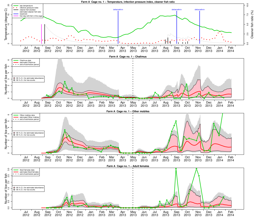
Figure 4: Fitted (until 15. May 2013) and predicted (from 16. May 2013) values for the lice and the cleaner fish populations. Symbols are as given in Figure 2 with the following additions: Upper panel: Fitted (posterior mean) cleaner fish ratio (dotted black curve). Three lower panels: i) Fitted values (red curves to the right of the vertical black dotted line), ii) predictions conditioned on known temperature, external infection pressure index and number and weight of salmon (red curves to the left of the vertical black dotted line), iii) corresponding 95% credible interval for the lice population (pink area) and iv) additional 95% credible interval for lice counts (grey area), i.e. including the randomness in the negative binomial distribution for lice counts.

There was substantial underreporting of the number of lice at the CH stage. Depending on the size of the fish, the model estimates suggested that on average only 9% to 19% of the CH lice were counted (Figure 5). In addition, there was substantial between farm variability in this counting error (Figure 5). The relationship between observed abundances of lice at the CH stage and predicted values was poorer than for the other stages (OM and AF), even when the underreporting was accounting for (the grey “counting error” area for CH in Figure 4 is wide and includes zero). This can be quantified by the aggregation parameter $\rho$ which was 50-75% lower than for OM and AF (Table 3). This indicates that the information content in the counts of CH stage lice is limited.

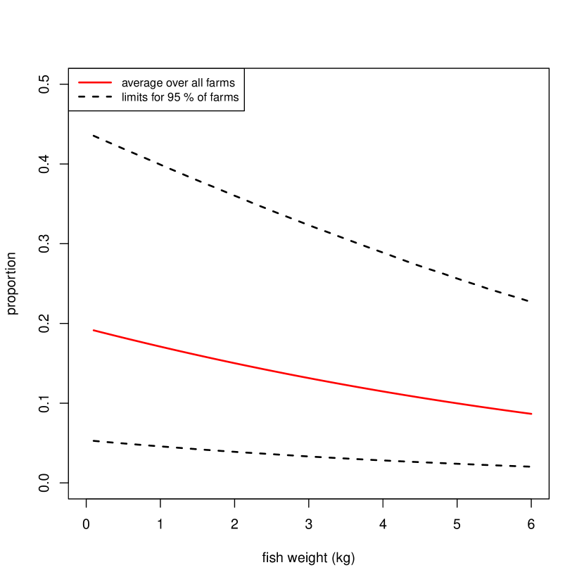
Figure 5: Posterior mean of the proportion of true CH lice counted as a function of fish weight, on average over all farms (solid line) and 95% limits for the between-farm variability (dashed lines).

3.2 Parameter estimates

Posterior mean estimates and credible intervals for parameters in the model are given in Tables 3 and 4. Note that for those parts of the model where we have no data, covariation between parameters in the model may lead to potential bias, i.e. high estimates of one parameter may be compensated for by an associated change in the value of another parameter. An example of this is that mortality and development rates for the R and CO stages and the reproduction rate are related, but without relevant observations to tease them apart. For instance, if the reproduction rate is overestimated, this can be compensated either by increasing the mortality in the R and CO stages (which are assumed to be equal) or by reducing the infection rate (development from CO to CH).

When compared to previously published estimates on stage-specific mortality, there are some notable differences (Table 5). The estimate of the mean mortality rate at the R and CO stages ($\lambda^{RCOnat}$) was higher than the previous estimate (Table 5). However, note that in our model, this quantity also accounts for nauplii and copepodids that drift away from the farm, in addition to the pure natural mortality. For the CH, PA and A stages, the mortality rates vary over time, but we calculated their overall expectations (averages in the long run) by simulation. The overall expectation for the mortality rate of the CH and PA stages tended to be towards the lower range of previous estimates, while the estimate for the adult stage was within the range of previous studies (Table 5). These estimates must be interpreted with caution since the model assumes equal development rates between genders and, furthermore, that adult males are pooled together with the PA stages in the observational data. More detailed figures on mortality, including parameter uncertainties, are presented in Figures 9-13 in the Supplementary material.

Table 3: Posterior means with 95% credible intervals of parameters in the static parts of the model.

Part of		Parameter	Parameter		Posterior	95% C.I.	95% C.I.
model	Stage	interpretation	symbol	Section	mean	lower	upper
Natural mortality	R,CO	Mortality rate	$\lambda^{RCOnat}$	2.4.3	0.303	0.293	0.314
Mortality cl.fish	PA, A	Regression coeff.	$\lambda^{clf}$	2.4.3	0.839	0.622	1.059
Development	Egg	Median at 10∘C	$\delta^{Em10}$	2.4.4	4.720	4.403	5.159
Development	Nauplii	Median at 10∘C	$\delta^{Nm10}$	2.4.4	4.096	3.646	4.421
Development	R	Shape parameter	$\delta^{Rs}$	2.4.4	18.865	16.027	19.975
Development	R	Power parameter	$\delta^{Rp}$	2.4.4	0.401	0.400	0.405
Development	CH	Median at 10∘C	$\delta^{CHm10}$	2.4.4	18.945	18.329	19.520
Development	CH	Shape parameter	$\delta^{CHs}$	2.4.4	8.024	7.120	8.976
Development	CH	Power parameter	$\delta^{CHp}$	2.4.4	1.299	1.252	1.344
Development	PA	Median at 10∘C	$\delta^{PAm10}$	2.4.4	10.700	10.126	11.257
Development	PA	Shape parameter	$\delta^{PAs}$	2.4.4	1.629	1.445	1.836
Development	PA	Power parameter	$\delta^{PAp}$	2.4.4	0.859	0.7806	0.937
Development	CO	Expectation	$\delta_{0}^{CO}$	2.4.5	-2.564	-2.970	-2.198
Development	CO	Regression coeff.	$\delta^{CO}_{1}$	2.4.5	0.084	0.043	0.125
Development	CO	Variance within farm	$(\sigma^{COdf})^{2}$	2.4.5	0.034	0.027	0.044
Development	CO	Variance between farms	$(\sigma^{COd})^{2}$	2.4.5	0.360	0.202	0.620
Reproduction	AF to R	Basic number of eggs	$\beta^{r}_{0}$	2.4.6	172.500	fixed
Reproduction	AF to R	Age dependence	$\beta^{r}_{1}$	2.4.6	0.200	fixed
Reproduction	AF to R	Density dependence	$\gamma^{r}$	2.4.6	493	481	498
Cleaner fish model		Mortality rate	$\kappa^{clf}$	2.5.1	0.027	0.022	0.034
Data model	CH	Aggregation parameter	$\rho^{CH}$	2.5.2	0.051	0.049	0.054
Data model	OM=PA+AM	Aggregation parameter	$\rho^{OM}$	2.5.2	0.194	0.183	0.206
Data model	AF	Aggregation parameter	$\rho^{AF}$	2.5.2	0.119	0.110	0.131
Data model	CH	Expectation	$\beta_{0}^{CHcount}$	2.5.2	-1.572	-1.832	-1.345
Data model	CH	Variance	$(\sigma^{CHcount})^{2}$	2.5.2	0.431	0.243	0.730
Data model	CH	Regression coeff.	$\beta^{CHcount}_{1}$	2.5.2	-0.164	-0.189	-0.135

Table 4: Posterior means with 95% credible intervals of parameters in the time-varying parts of the model.

Part of		Parameter	Parameter		Posterior	95% C.I.	95% C.I.
model	Stage	interpretation	symbol	Section	mean	lower	upper
Natural mortality	CH	Expectation in AR(1)	$\lambda_{0}^{CHnat}$	2.4.3	-6.943	-7.043	-6.847
Natural mortality	CH	Coefficient in AR(1)	$\phi^{CHnat}$	2.4.3	0.011	0.001	0.027
Natural mortality	CH	Variance in AR(1)	$(\sigma^{CHnat})^{2}$	2.4.3	0.019	0.011	0.026
Natural mortality	PA	Expectation in AR(1)	$\lambda_{0}^{PAnat}$	2.4.3	-4.908	-5.040	-4.713
Natural mortality	PA	Coefficient in AR(1)	$\phi^{PAnat}$	2.4.3	0.025	0.001	0.065
Natural mortality	PA	Variance in AR(1)	$(\sigma^{PAnat})^{2}$	2.4.3	0.130	0.099	0.173
Natural mortality	A	Expectation in AR(1)	$\lambda_{0}^{Anat}$	2.4.3	-2.411	-2.492	-2.332
Natural mortality	A	Coefficient in AR(1)	$\phi^{Anat}$	2.4.3	0.693	0.676	0.708
Natural mortality	A	Variance in AR(1)	$(\sigma^{Anat})^{2}$	2.4.3	0.729	0.685	0.775
Mortality ch.tr.	CH, PA, A	Expectation, deltamethrin	$\lambda^{DMcht}$	2.4.3	2.400	1.641	3.145
Mortality ch.tr.	CH, PA, A	Variance, deltamethrin	$(\sigma^{DMcht})^{2}$	2.4.3	9.070	6.031	12.427
Mortality ch.tr.	PA, A	Expectation, azamethiphos	$\lambda^{AZcht}$	2.4.3	0.133	-0.675	1.007
Mortality ch.tr.	PA, A	Variance, azamethiphos	$(\sigma^{AZcht})^{2}$	2.4.3	$(\sigma^{DMcht})^{2}$
Mortality ch.tr.	PA, A	Expectation, H2O2	$\lambda^{HPcht}$	2.4.3	4.056	3.219	5.159
Mortality ch.tr.	PA, A	Variance, H2O2	$(\sigma^{HPcht})^{2}$	2.4.3	$(\sigma^{DMcht})^{2}$
Mortality ch.tr.	CH, PA, A	Expectation, emamectin	$\lambda^{EMcht}$	2.4.3	-4.744	-5.456	-4.280
Mortality ch.tr.	CH, PA, A	Variance, emamectin	$(\sigma^{EMcht})^{2}$	2.4.3	1.825	0.865	3.483
Mortality ch.tr.	CH, PA	Expectation, diflubenzuron	$\lambda^{DIcht}$	2.4.3	-8.712	-12.555	-4.638
Mortality ch.tr.	CH, PA	Variance, diflubenzuron	$(\sigma^{DIcht})^{2}$	2.4.3	$(\sigma^{EMcht})^{2}$
External recr.	AF to R	Expectation in AR(1)	$\mu^{Ext}$	2.5	0.300	0.182	0.411
External recr.	AF to R	Coefficient in AR(1)	$\phi^{Ext}$	2.5	0.934	0.924	0.944
External recr.	AF to R	Variance in AR(1)	$(\sigma^{Extar})^{2}$	2.5	0.164	0.152	0.175
External recr.	AF to R	Variance	$(\sigma^{Ext})^{2}$	2.5	0.007	0.001	0.027

Table 5: Posterior means with 95% credible intervals of daily mortality from this study together with point estimates or ranges from previous studies.

	Point
	estimate
Stage	or range	95% C.I.	Sex	Comment	Reference
nauplii	0.30	0.29-0.31		for R=eggs+nauplii, includes drifting away	this paper
	0.17			“plausible value”	Stien et al. (2005)
CO	0.30	0.29-0.31		same as for R	this paper
	0.22			”plausible values”	Stien et al. (2005)
CH	0.0010	0.0009-0.0011			this paper
	0.002-0.01			”plausible values”	Stien et al. (2005)
	0.0006-0.020			outer interval limits from 4 reported studies	–”–
	0.0002-0.026			range over 7 trials on juvenile Pacific salmon	Krkošek et al. (2009)
PA	0.0079	0.0068-0.0096			this paper
	0.02-0.18		males	”plausible values”	Stien et al. (2005)
	0.002-0.21		males	outer interval limits from 4 reported studies	–”–
	0.03-0.07		females	”plausible values”	–”–
	0.011-0.102		females	outer interval limits from 4 reported studies	–”–
	0.14-0.34			PA+A combined,range over 7 trials	Krkošek et al. (2009)
				on juvenile Pacific salmon
A	0.12	0.11-0.13			this paper
	0.03-0.06		males	”plausible values”	Stien et al. (2005)
	0.008-0.26		males	outer interval limits from 4 reported studies	–”–
	0.02-0.04		females	”plausible values”	–”–
	0.003-0.70		females	outer interval limits from 3 reported studies	–”–
	0.14-0.34			PA+A combined,range over 7 trials	Krkošek et al. (2009)
				on juvenile Pacific salmon

We also used simulations to find the estimated median development times, since the $\delta^{m10}$ parameters given in Table 3 have exact interpretations only in the continuous Weibull distribution. Estimated median development times at 10^∘C were similar to mean and minimum estimates from previous studies (Table 6), however with a slightly higher estimate at the CH stage and fairly low estimate for the PA stage. Panel a) in Figure 6 shows how the estimated development rates increases by stage-age at a temperature of 10^∘C. These curves differ in principle from the development rates used in all population models mentioned in Section 2.1, since all these models use step functions with a development rate of 0 until a minimum development time and then a constant rate afterwards. For the R and CH stages, however, the estimated cumulative proportion of lice developed to the next stage (panel b) in Figure 6) resembel these step functions. For the PA stage, however, the estimated development rate is fundamentally different from those used in other models, since the estimated development rate for PA is non-zero already after one day. This implies that some lice in the PA stage may develop to the A stage very quickly in the present model.

Note that these curves ignore mortality, and the cumulative mortalities may be high for stage-ages where the development rates still are quite low, especially at low temperatures. More detailed figures on development times, including parameter uncertainties and for different temperatures (5, 10 and 15^circC), are presented in Figures 14-16 in the Supplementary material.

Table 6: Posterior means with 95% credible intervals of development times (in days) at 10^∘C from this study together with point estimates or ranges from previous studies.

	Point
	estimate		Estimate
Stage	or range	95% C.I.	of what	Sex	Comment	Reference
eggs	4.8	4.5-5.3	median			this paper
	8.8		minimum		from their Eq. (8) and Table 3	Stien et al. (2005)
	4.6		mean			Samsing et al. (2016)
nauplii	4.2	3.7-4.5	median			this paper
	3.6		minimum		from their Eq. (8) and Table 3	Stien et al. (2005)
	3.8		mean			Samsing et al. (2016)
CH	18.8	18.0-19.0	median			this paper
	15.4		minimum	males	from their Eq. (8) and Table 3	Stien et al. (2005)
	16.5		minimum	females	from their Eq. (8) and Table 3	Stien et al. (2005)
	11-13		range	males		Eichner et al. (2015)
	13-15		range	females		Eichner et al. (2015)
	11-14		minimum		5 trials on juvenile Pacific salmon at 9-11∘C	Krkošek et al. (2009)
PA	10.5	10.0-11.0	median			this paper
	10.4		minimum	males	calculated as difference of their time	Stien et al. (2005)
					from CH to A and from CH to PA
	15.4		minimum	females	calculated as difference of their time	Stien et al. (2005)
					from CH to A and from CH to PA

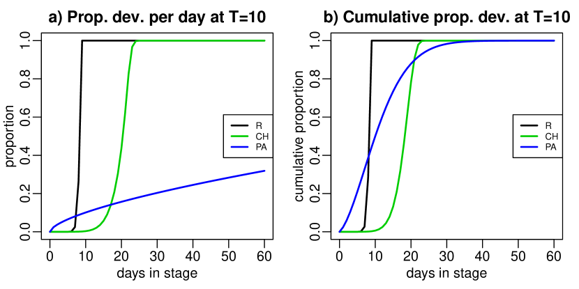
Figure 6: Posterior means of daily development (a) and cumulative proportion developed to next stage (b) at temperature 10 for stages R, CH and PA. The curves are the posterior means of the development rates, conditioned on each stage-age, and may therefore be slightly different from curves based the posterior means of the parameter values plugged into Eq. (27).

We obtain an estimate of the daily cleaner fish mortality of 0.027 (C.I. 0.022-0.034, Table 3). This suggest that the cleaner fish population is reduced to its half about 1 month after release. The model confirms that there is increased mortality of lice associated with the use of cleaner fish (Figure 7 and Table 3). With a 10% cleaner fish to salmon ratio, the estimated daily lice mortality (for lice in the PA and A stages) due to the use of cleaner fish, is 0.080 (C.I. 0.060-0.100). This implies a reduction in the life expectancy for adult lice from 8.5 to 5 days with an increase in cleaner fish ratio from 0 to 10%, and a decrease in the life expectancy for pre-adult lice (PA) going from 127 days to 11 days for the same change in cleaner fish ratio. Therefore, in particular for PA lice, the use of cleaner fish is estimated to have a substantial effect on lice survival. However, in the present data, the (estimated) cleaner fish ratio seldom amounted stocked to more than 5%, which seems to be too low to avoid additional treatments, since medical treatments were applied in almost all cages in the data set.

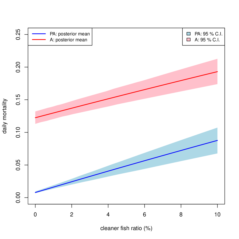
Figure 7: Posterior mean and 95% credible intervals for the total mortality for the PA and A stages when the cleaner fish ratio is increased from 0 (only natural mortality) to 10%.

The effects of the various chemotherapeutic treatments are difficult to compare since the assumed duration of the effects varies between treatments and by temperature, and because they affect different stages of lice. Furthermore, since lice develop resistance towards such treatments (Aaen et al., 2015), we expect that the effect will decrease over time. Nevertheless, the estimated expected cumulative mortality of lice (found by simulation) in the PA or A stages due to bath treatments (i.e. non-feed) ten days post treatment at 10^∘C, were high for hydrogen peroxide (0.99, C.I. 0.97-1.00), and deltamethrin/cypermethrin (0.94 , C.I. 0.88-0.97) and somewhat lower for azamethiphos (0.74 , C.I. 0.64-0.85). The first two of these are similar to what others have reported for non-resistant lice populations, being 99% for hydrogen peroxide (Groner et al., 2013) and 95% for deltamethrin and cypermethrin (Revie et al., 2005). The estimated effects of all treatment types are further illustrated in Figures 9-13 in the Supplementary material.

Both external and internal recruitment varied substantially over time, and one of the two may dominate the other in certain periods. The estimated proportion of internal recruitment for each farm averaged over the whole production cycle varies from about 4 to 73%. On average over all farms, this proportion is 24% (C.I. 23-26%), with a median of 19. This is in accordance with results in Ådlandsvik (2015), who reported a median of 18% for the proportion of internal recruitment, based on a simulation of the spread of lice larvae between 591 farms from a hydrodynamic model that takes sea currents into account (Johnsen et al., 2014). When the abundance of adult female lice was low in the farm, naturally internal recruitment tended to be low, while internal recruitment was estimated to be very important in farms with a high abundance of adult females (Figure 8).

Figure 8: Posterior mean of the average proportion of recruitment that has an internal source as a function of abundance of adult females, averaged over all farms and all time points.

Concerning the reproduction rate, we notice that the estimate of $\gamma^{r}_{0}$ is 493 (C.I 481-498). In practice, this means that there is no evidence of density dependent reproductive rates (Allee effect) in the estimated model, contrary to the hypothesis suggested by Stormoen et al. (2013), Krkošek et al. (2012) and Groner et al. (2014). One reason for this discrepancy is that recruitment from external sources is not considered in the aforementioned models. In our model, internal recruitment is on average of less importance than external recruitment at low abundances of AF lice. Reduced reproductive rates at low abundances of infection are therefore likely to be masked by external recruitment.

4 Conclusion

The presented process model for the population dynamics of salmon lice in aquaculture farm systems combine 1) a model for the main stage structure of salmon lice; 2) model terms that describe internal and external recruitment of salmon lice to the farms; 3) models for the impact of a management strategies adopted to reduce and control salmon lice infection levels; and 4) allows for stochasticity in aspects of these processes. In addition, we describe a model for the link between the process model and data collected on a routine basis in modern aquaculture. This allows the process model to be fitted to data and updated when new production and salmon lice data from fish farms become available. The model produces estimates of lice abundances in fish farms that correspond well with observed infection levels. Furthermore, it allows reasonable predictions of pre-adult and adult sea lice infection levels to be made for several weeks into the future (Figure 4). We note, however, that the observational data on the number of lice at the chalimus stage vary substantially, and is underestimated to varying degrees between fish farms. This suggests that the data collected on the abundance of lice at the chalimus stages contain limited information in terms of real infection levels in the farms.

The model generates stage specific estimates of development and mortality rates based on real production data. For the planktonic stages, the estimates of mortality rates were high relative to earlier field and laboratory studies, but these are not directly comparable, since our definition of mortality include lice that drift away from the farm. For the chalimus and pre-adult stages, the mortality rates were low compared to previous studies, while it was rather high for the adult stage. One reason could be the poor data support for the early life stages, since we have no data on the planktonic stages and poor data on the chalimus stages. The poor support by data makes it difficult to separate survival-estimates at these stages from other parameters in the model, in particular reproduction rates, development rates and biases in chalimus counts, and perhaps this problem propagates to the pre-adult stage. The median development times for are reasonable. However, we note that the distribution of development times from the pre-adult to the adult stages include the possibility of very short development times. It is unclear why this happens, but one possible explanation could be movement of adult lice between cages within a fish farm. Another explanation could be that some of the non-gravid female adults have been misclassified as pre-adults in the lice count data.

The model is well suited to quantify the effect of different treatments on lice infection levels. This aspect may be useful in monitoring development of resistance to treatments in sea lie populations. Furthermore, to our knowledge this is a first data-based quantification of the effect of using cleaner fish to manage lice levels in full scale salmon farms.

The model allows both internal and external infection processes to be quantified. When there are no adult female lice in a fish farm, all new infections will necessarily come from external sources. When reproducing adult female lice are present, however, they may contribute substantially to infection pressure at the farm. Their impact on local recruitment will depend both on their numbers and their reproductive rate, but also on the external infection pressure. The model did not suggest any evidence of density dependent reproductive rates.

The emphasis on salmon louse control in salmon farming has gravely intensified in later years, resulting in the implementation of a variety of innovative control methods. Some of these methods aim to reduce salmon louse recruitment from external sources, whereas other methods aim at increasing the mortality of parasitic stages of the lice, such as the use of cleaner fish. To tease out actual effects of such control efforts at farm levels, or more so for farms in a production area, is not a simple task, given the interconnected production-system of fish farms and planktonic spread of this parasite. The present model for the population dynamics of salmon lice in aquaculture farm systems may resolve the complexity of processes to a degree that will improve evaluations of effects of various control efforts at farm levels. We believe that using the model as “mathematical laboratory” to explore effects of different salmon louse control strategies in interconnected farms in production areas has a large potential for rationalising area-wise control strategies in an informed manner.

References

- Aaen et al. (2015) Aaen S, Helgesen K, Bakke M, Kaur K, Horsberg T. 2015. Drug resistance in sea lice: A threat to salmonid aquaculture. Trends in Parasitology 31: 72–81, doi:10.1016/j.pt.2014.12.006.
- Aalen et al. (2008) Aalen O, Borgan Ø, Gjessing H. 2008. Survival and event history analysis - A process point of view, Springer, New York.
- Ådlandsvik (2015) Ådlandsvik B 2015. Forslag til produksjonsområder (in Norwegian). Tech. rep., Institute of Marine Research, Bergen, Norway, report from IMR no. 20-2015.
- Aldrin et al. (2015) Aldrin M, Huseby R, Jansen P. 2015. Space-time modelling of the spread of pancreas disease (PD) within and between Norwegian marine salmonid farms. Prev Vet Med 121: 132–141, doi:10.1016/j.prevetmed.2015.06.005.
- Aldrin et al. (2011) Aldrin M, Lyngstad T, Kristoffersen A, Storvik B, Borgan Ø, Jansen P. 2011. Modelling the spread of infectious salmon anaemia (ISA) among salmon farms based on seaway distances between farms and genetic relationships between ISA virus isolates. J R Soc Interface 8: 1346–1356.
- Aldrin et al. (2010) Aldrin M, Storvik B, Frigessi A, Viljugrein H, Jansen P. 2010. A stochastic model for the assessment of the transmission pathways of heart and skeleton muscle inflammation, pancreas disease and infectious salmon anaemia in marine fish farms in Norway. Prev Vet Med 93: 51–61, doi:10.1016/j.prevetmed.2009.09.010.
- Aldrin et al. (2013) Aldrin M, Storvik B, Kristoffersen A, Jansen P. 2013. Space-time modelling of the spread of salmon lice between and within Norwegian marine salmon farms. PLoS ONE 8: e64039, doi:10.1371/journal.pone.0064039.
- Anonymous (2015) Anonymous. 2015. Forutsigbar og miljømessig bærekraftig vekst i norsk lakse- og ørretoppdrett (in Norwegian), The Norwegian Ministry of Trade, Industry and Fisheries, Oslo.
- Brooks-Pollock et al. (2014) Brooks-Pollock E, Roberts G, Keeling M. 2014. A dynamic model of bovine tuberculosis spread and control in Great Britain. Nature 511, doi:10.1038/nature13529.
- Diggle (2006) Diggle P. 2006. Spatio-temporal point processes, partial likelihood, foot and mouth disease. Stat Methods Med Res 15: 325–336, doi:10.1191/0962280206sm454oa.
- Eichner et al. (2015) Eichner C, Hamre L, Nilsen F. 2015. Instar growth and molt increments in Lepeophtheirus salmonis (Copepoda: Caligidae) chalimus larvae. Parasitology International 64: 86–96, doi:10.1016/j.parint.2014.10.006.
- Gettinby et al. (2011) Gettinby G, Robbins C, Lees F, Heuch P, Finstad B, Malkenes R, Revie C. 2011. Use of a mathematical model to describe the epidemiology of Lepeophtheirus salmonis on farmed Atlantic salmon Salmo Salar in the Hardangerford, Norway. Aquaculture 320: 164–170, doi:10.1016/j.aquaculture.2011.03.017.
- Gilks et al. (1996) Gilks W, Richardson S, Spiegelhalter De. 1996. Markov Chain Monte Carlo in Practice, Chapman & Hall/CRC, Boca Raton.
- Groner et al. (2013) Groner M, Cox R, Gettinby G, Revie C. 2013. Use of agent-based modelling to predict benefits of cleaner fish in controlling sea lice, Lepeophtheirus salmonis, infestations on farmed Atlantic salmon, Salmo Salar L. Journal of Fish Diseases 36: 195–208, doi:10.1111/jfd.12017.
- Groner et al. (2014) Groner M, Gettinby G, Stormoen M, Revie C, Cox R. 2014. Modelling the Impact of Temperature-Induced Life History Plasticity and Mate Limitation on the Epidemic Potential of a Marine Ectoparasite. PLoS ONE 9: e88465, doi:10.1371/journal.pone.0088465.
- Groner et al. (2016) Groner M, McEwan G, Rees E, Gettinby G, Revie C. 2016. Quantifying the influence of salinity and temperature on the population dynamics of a marine ectoparasite. Canadian Journal of Fisheries and Aquatic Science 73: 1:11, doi:10.1139/cjfas-2015-0444.
- Hamre et al. (2013) Hamre L, Eichner C, Caipang C, Dalvin S, Bron J, Nilsen F, Boxshall G, Skern-Mauritzen R. 2013. The salmon louse Lepeophtheirus salmonis (Copepoda:Caligidae) life cycle has only two chalimus stages. PLoS ONE 8: e73539.
- Höhle (2009) Höhle M. 2009. Additive-Multiplicative Regression Models for Spatio-Temporal Epidemics. Biom J 51: 961–978, doi:10.1002/bimj.200900050.
- Jansen et al. (2012) Jansen P, Kristoffersen A, Viljugrein H, Jimenez D, Aldrin M, Stien A. 2012. Sea lice as a density dependent constraint to salmonid farming. Proc R Soc B Doi:10.1098/rspb.2012.0084.
- Johnsen et al. (2014) Johnsen I, Fiksen O, Sandvik A, Asplin L. 2014. Vertical salmon lice behaviour as a response to environmental conditions and its influence on regional dispersion in a fjord system. Aquacult Environ Interact 5: 127–141, doi:10.3354/aei00098.
- Jonkers et al. (2010) Jonkers A, Sharkey K, Thrush M, Turnbull J, Morgan K. 2010. Epidemics and control strategies for diseases of farmed salmonids: A parameter study. Epidemics 2: 195–206, doi:10.1016/j.epidem.2010.08.001.
- Keeling et al. (2001) Keeling M, Woolhouse M, Shaw D, Matthews L, Chase-Topping M, Haydon D, Cornell S, Kappey J, Wilesmith, J., Grenfell B. 2001. Dynamics of the 2001 UK foot and mouth epidemic: stochastic dispersal in a heterogeneous landscape. Science 294: 813–817.
- Kristoffersen et al. (2014) Kristoffersen A, D. J, Viljugrein H, Grøntvedt R, Stien A, Jansen P. 2014. Large scale modelling of salmon lice (Lepeophtheirus salmonis) infection pressure based on lice monitoring data from Norwegian salmonid farms. Epidemics 9: 31–39, doi:10.1016/j.epidem.2014.09.007.
- Kristoffersen et al. (2013) Kristoffersen A, Rees E, Stryhn H, R. I, Campisto J, Revie C, St-Hilaire S. 2013. Understanding sources of sea lice for salmon farms in Chile. Prev Vet Med 111: 165–175, doi:10.1016/j.prevetmed.2013.03.015.
- Kristoffersen et al. (2009) Kristoffersen A, Viljugrein H, Kongtorp R, Brun E, Jansen P. 2009. Risk factors for pancreas disease (PD) outbreaks in farmed Atlantic salmon and rainbow trout in Norway during 2003-2007. Prev Vet Med 90: 127–136.
- Krkošek et al. (2010) Krkošek M, Bateman A, Proboszcz S, Orr C. 2010. Dynamics of outbreak and control of salmon lice on two salmon farms in the Broughton Archipelago. Aquacult Environ Interact 1: 137–146, doi:10.3354/aei00014.
- Krkošek et al. (2012) Krkošek M, Connors B, Lewis M, Poulin R. 2012. Allee Effects May Slow the Spread of Parasites in a Coastal Marine Ecosystem. The American Naturalist 179: 401–412, doi:10.5061/dryad.34g16868.
- Krkošek et al. (2007) Krkošek M, Ford J, Morton A, Lele S, Myers R, Lewis M. 2007. Declining wild salmon populations in relation to parasites from farm salmon. Science 318: 1772–1775, doi:10.1126/science.1148744.
- Krkošek et al. (2009) Krkošek M, Morton A, Volpe J, Lewis M. 2009. Sea lice and salmon population dynamics: effects of exposure time for migratory fish. Proc R Soc BScience 276: 2819–2828, doi:10.1098/rspb.2009.0317.
- Leclercq et al. (2014) Leclercq E, Davie A, Migaud H. 2014. Delousing efficiency of farmed ballan wrasse (Labrus bergylta) against Lepeophtheirus salmonis infecting Atlantic salmon (Salmo salar) post-smolts. Pest Management Science 70: 1274–1282, doi:10.1002/ps.3692.
- Murray and Salama (2016) Murray A, Salama N. 2016. A simple model of the role of area management in the control of sea lice. Ecological Modelling 337: 39–47, doi:10.1016/j.ecolmodel.2016.06.007.
- Nygaard (2010) Nygaard S 2010. Slides - Lusekurs for røktere - Bokn 26. mars 2010. Tech. rep., Fiskehelse og Miljø AS.
- Ottesen et al. (2012) Ottesen K, Rykhus K, et al. 2012. Terapiveileder - Medikamentell behandling mot lus, revidert utgave våren 2012. Tech. rep., Arbeidesgruppe.
- Revie et al. (2005) Revie C, Robbins C, Gettinby G, Kelly L, Treasurer J. 2005. A mathematical model of the growth of sea lice, Lepeophtheirus salmonis, populations on farmed Atlantic salmon, Salmo Salar L., in Scotland and its use in the assessment of treatment strategies. Journal of Fish Diseases 28: 603–613.
- Rittenhouse et al. (2016) Rittenhouse M, Revie C, Hurford A. 2016. A model for sea lice (Lepeophtheirus salmonis) dynamics in a seasonally changing environment. Epidemics 16: 8–16, doi:10.1016/j.epidem.2016.03.003.
- Salama and Murray (2013) Salama N, Murray A. 2013. A comparison of modelling approaches to assess the transmission of pathogens between Scottish fish farms: The role of hydrodynamics and site biomass. Preventive Veterinary Medicine 108: 285–293, doi:10.1016/j.prevetmed.2012.11.005.
- Samsing et al. (2016) Samsing F, Oppedal F, Dalvin S, Johnsen I, Vågseth T, Dempster T. 2016. Salmon lice (Lepeophtheirus salmonis) development times, body size, and reproductive outputs follow universal models of temperature dependence. Canadian Journal of Fisheries and Aquatic Science 73: 1–11??? NOT FINAL, doi:10.1139/cjfas-2016-0050.
- Scheel et al. (2007) Scheel I, Aldrin M, Frigessi A, Jansen P. 2007. A stochastic model for infectious salmon anemia (ISA) in Atlantic salmon farming. J R Soc Interface 4: 699–706.
- Stien et al. (2005) Stien A, Bjørn P, Heuch P, Elston D. 2005. Population dynamics of salmon lice Lepeophtheirus salmonis on Atlantic salmon and sea trout. Mar Ecol Prog Ser 290: 263–275.
- Stormoen et al. (2013) Stormoen M, Skjerve E, Aunsmo A. 2013. Modelling salmon lice, Lepeophtheirus salmonis, reproduction on farmed Atlantic salmon, Salmo salar L. Journal of Fish Diseases 36: 25–33.