Hybrid Kinematic Control for Rigid Body Pose Stabilization using Dual Quaternions

Abstract

In this paper, we address the rigid body pose stabilization problem using dual quaternion formalism. We propose a hybrid control strategy to design a switching control law with hysteresis in such a way that the global asymptotic stability of the closed-loop system is guaranteed and such that the global attractivity of the stabilization pose does not exhibit chattering, a problem that is present in all discontinuous-based feedback controllers. Using numerical simulations, we illustrate the problems that arise from existing results in the literature—as unwinding and chattering—and verify the effectiveness of the proposed controller to solve the robust global pose stability problem.

1 Introduction

Rigid body motion and its control have been extensively investigated in the last forty years because of its applications in the theory of mechanical systems, such as robotic manipulators, satellites and mobile robots. Research has largely focused on the study of models and control strategies in the Lie group of rigid body motions $\textrm{SE}(3)$ and its subgroup $\textrm{SO}(3)$ of proper rotations [1, 2, 3, 4].

Although it is usual to design attitude and rigid motion controllers for mechanical systems respectively using rotation matrices and homogeneous transformation matrices (HTM) [3], it has been noted by some authors that a non-singular representation, namely the unit quaternion group $\text{Spin}(3)$ for rotations and the unit dual quaternions $\text{Spin}(3)\ltimes\mathbb{R}^{3}$ for rigid motions can bring computational advantages [4, 5, 6].

In scenarios where the state space of the dynamical system is not the Euclidean space $\mathbb{R}^{n}$ but a general differentiable manifold $\mathcal{M}$—which is the case of $\textrm{SE}(3)$ and $\text{Spin}(3)\ltimes\mathbb{R}^{3}$—some difficulties in designing a stabilizing closed-loop controller may arise. For instance, the topology of $\mathcal{M}$ may obstruct the existence of a globally asymptotically stable equilibrium point in any continuous vector field defined on $\mathcal{M}$: in [1] it is proved that if $\mathcal{M}$ has the structure of a vector bundle over a compact manifold $\mathcal{L}$, then no continuous vector field on $\mathcal{M}$—indeed, nor in $\mathcal{L}$—has a globally asymptotically stable equilibrium. In particular, this means that it is impossible to design a continuous feedback that globally stabilizes the pose of a rigid body, as in this case the closed-loop system state space manifold is a trivial bundle over the compact manifold $\textrm{SO}(3)$. The same topological obstruction is also present in the group of unit dual quaternions since its underlying manifold is a trivial bundle over the unit sphere $\mathcal{S}^{3}$ (see Theorem 1 in Subsection 2.3).

On the other hand, due to the two-to-one covering map $\text{Spin}(3)\ltimes\mathbb{R}^{3}\rightarrow\textrm{SE}(3)$, the unit dual quaternion group is endowed with a double representation for every pose in $\textrm{SE}(3)$. Neglecting the double covering yields to the problem of unwinding whereby solutions close to the desired pose in $\textrm{SE}(3)$ may travel farther to the antipodal unit dual quaternion representing the same pose [7]. There are few works on unwinding avoidance in the context of pose stabilization using unit dual quaternions [7, 8, 9, 10]. All of them are based on a discontinuous sign-based feedback approach.

As shown by [11] for the particular case of $\text{Spin}(3)$, the discontinuous sign-based approach may, however, be particularly sensitive to measurement noises, and despite achieving global stability, global attractivity properties may be detracted with arbitrarily small measurement noises. As one would expect, the same happens with $\text{Spin}(3)\ltimes\mathbb{R}^{3}$ and this will be shown in Theorem 1.

As verified in Section 3, in $\text{Spin}(3)\ltimes\mathbb{R}^{3}$ the lack of robustness is even more relevant as the discontinuity of the controller not only affects the rotation, but may also disturb and deteriorate the trajectory of the system translation. In this context, even extremely small noises may lead to chattering, performance degradation—and in the worst case, prevent stability. Summing up, despite the solid contributions in the literature on dual quaternion based controllers in the context of rigid body motion stabilization, tracking, and multi-agent coordination [8, 7, 9, 12, 13, 14, 15, 10], control of manipulators and human-robot interaction [16, 17, 18, 19, 20, 21], and satellite and spacecraft tracking [22, 23, 24], it is important to emphasize that existing pose controllers are either stable only locally (as we show in Section 2) or have lack of robustness in the sense that they are sensitive to arbitrarily small measurement noises (as we illustrate in Section 5). In other words, the topological constraints from $\text{Spin}(3)\ltimes\mathbb{R}^{3}$, most of them inherited from $\textrm{SE}(3)$, still pose a challenge—the extension from results on attitude control to the problem of pose control is not trivial— and there exists no result in the literature that ensures robust global stability.

Contributions

In this paper, a generalized robust hybrid control strategy for the global stabilization of rigid motion kinematics within unit dual quaternions framework is proposed. The strategy stems from the idea of the hybrid kinematic control law with hysteresis switching proposed in [11] to solve the non-robustness issue for quaternions. It is important to emphasize that, albeit some algebraic identities in quaternion algebra can be easily carried over to the dual quaternion algebra by the principle of transference [25, 4], the proposed generalization does not follow by the principle of transference. In fact, counterexamples shown in [25] illustrate the failure of the transfer principle outside the algebraic realm.

In summary, whereas unit quaternions are used to model only attitude and perform a double cover for the Lie group $\textrm{SO}(3)$, unit dual quaternions model the coupled attitude and position and perform a double cover for the Lie group $\textrm{SE}(3)$. The necessity of different procedures for quaternion and dual quaternion stems from their different topologies and group structures. For example, the unit quaternion group is a compact manifold, whereas the unit dual quaternion group is not a compact manifold. This reflects in the use of distinct approaches to controller design (see for instance [3]). It is also interesting to highlight that due to $\textrm{SO}(3)$ being compact, it has a natural bi-invariant metric, but the same can not be said from $\textrm{SE}(3)$ as it does not possess any bi-invariant metric. The unit dual quaternion group is not a subgroup from $\text{Spin}(3)$—it is indeed the other way around—and boundedness, geodesic distance, norm properties, and other manifold features that are valid on $\mathcal{S}^{3}$ cannot be directly carried to $\text{Spin}(3)\ltimes\mathbb{R}^{3}$. In this sense, the extension of control results to $\text{Spin}(3)\ltimes\mathbb{R}^{3}$ is not trivial, which is reflected by the gap between quaternion based results and dual quaternion based controllers—where the double covering map is often neglected [12, 13, 15, 14, 6]. To overcome this context, we introduce a novel Lyapunov function that exploits the algebraic constraints inherent from the unit dual quaternion manifold, and a new robust hybrid stabilization controller for rigid motion using $\text{Spin}(3)\ltimes\mathbb{R}^{3}$ is derived.

Notation

Lowercase bold letters represent quaternions, such as $\boldsymbol{q}$. Underlined lower case bold letters represent dual quaternions, such as $\underline{\boldsymbol{q}}$. The following notations will also be used:

$\mathbb{R}$	set of real numbers;
$\mathbb{R}_{\geq 0}$	set of non-negative real numbers;
$\mathbb{B}$	closed unit ball in the Euclidean norm;
$\mathbb{H}$	set of quaternions;
$\mathbb{H}_{0}$	set of pure imaginary quaternions;
$\mathbb{H}\otimes\mathbb{D}$	set of dual quaternions;
$\textrm{SO}(3)$	$3$-dimensional Lie group of rotations;
$\textrm{SE}(3)$	$3$-dimensional Lie group of rigid body motions;
$\text{Spin}(3)$	Lie group of unit norm quaternions;
$\text{Spin}(3)\ltimes\mathbb{R}^{3}$	Lie group of unit norm dual quaternions;
$\mathcal{S}^{3}$	underlying manifold of unit norm quaternions;
$\underline{\boldsymbol{S}}$	underlying manifold of unit norm dual quaternions;
$\mathcal{KL}$	class of continuous functions $\beta:\mathbb{R}_{\geq 0}\times\mathbb{R}_{\geq 0}\rightarrow\mathbb{R}_{\geq 0}$
	such that for each fixed $s$, the function $\beta\left(r,s\right)$ is
	strictly increasing and $\beta\left(0,s\right)=0$ and for each fixed $r$,
	the function $\beta\left(r,s\right)$ is decreasing and $\lim_{s\rightarrow\infty}\beta\left(r,s\right)=0$;
$\|\cdot\|$	Euclidean norm;
$\boldsymbol{u}\cdot\boldsymbol{v}$	dot product between pure imaginary quaternions $\boldsymbol{u}$ and $\boldsymbol{v}$;
$\boldsymbol{u}\times\boldsymbol{v}$	cross product between pure imaginary quaternions $\boldsymbol{u}$ and $\boldsymbol{v}$;
$\overline{\mathrm{co}}(\cdot)$	closure of the convex hull;
$X+Y$	Minkowski sum between the sets $X$ and $Y$;
$x^{+}$	denotes the next state of the hybrid system after a jump;

2 Preliminaries

In this section, we provide for the reader basic concepts and a brief theoretical background regarding quaternions and dual quaternion representation for rigid body motion. We also present the topological constraints—which affect any mathematical structure that represents rigid motion—imposed by dual quaternions.

2.1 Quaternions

The quaternion algebra is a four-dimensional associative division algebra over $\mathbb{R}$ introduced by Hamilton [26] to algebraically express rotations in the three-dimensional space. The elements $1$,$\hat{\imath},\hat{\jmath},\hat{k}$ are the basis of this algebra, satisfying

$$\hat{\imath}^{2}=\hat{\jmath}^{2}=\hat{k}^{2}=\hat{\imath}\hat{\jmath}\hat{k}=-1,$$

and the set of quaternions is defined as

$$\smash{\mathbb{H}\triangleq\biggl{\{}\eta+\text{$\hat{\imath}$}\mu_{1}+\hat{\jmath}\mu_{2}+\hat{k}\mu_{3}:\eta,\mu_{1},\mu_{2},\mu_{3}\in\mathbb{R}\biggr{\}}.}$$

Consider a quaternion $\boldsymbol{q}=\eta+\text{$\hat{\imath}$}\mu_{1}+\hat{\jmath}\mu_{2}+\hat{k}\mu_{3}$; for ease of notation, it may be denoted as

$$\smash{\boldsymbol{q}=\eta+\boldsymbol{\mu},\quad\text{with }\quad\boldsymbol{\mu}=\text{$\hat{\imath}$}\mu_{1}+\hat{\jmath}\mu_{2}+\hat{k}\mu_{3}.}$$

In addition, it may be decomposed into a real component and an imaginary component: $\operatorname{\mathrm{Re}}\left(\boldsymbol{q}\right)\triangleq\eta$ and $\operatorname{\mathrm{Im}}\left(\boldsymbol{q}\right)\triangleq\boldsymbol{\mu}$, such that $\boldsymbol{q}=\operatorname{\mathrm{Re}}\left(\boldsymbol{q}\right)+\operatorname{\mathrm{Im}}\left(\boldsymbol{q}\right)$. The quaternion conjugate is given by $\boldsymbol{q}^{*}\triangleq\operatorname{\mathrm{Re}}\left(\boldsymbol{q}\right)-\operatorname{\mathrm{Im}}\left(\boldsymbol{q}\right)$. Pure imaginary quaternions are given by the set

$$\mathbb{H}_{0}\triangleq\left\{\boldsymbol{q}\in\mathbb{H}:\;\operatorname{\mathrm{Re}}\left(\boldsymbol{q}\right)=0\right\}$$

and are very convenient to represent vectors of $\mathbb{R}^{3}$ within the quaternion formalism by means of a trivial isomorphism, which implies $\mathbb{H}_{0}\cong\mathbb{R}^{3}$. Both cross product and dot product are defined for elements of $\mathbb{H}_{0}$ and they are analogous to their counterparts in $\mathbb{R}^{3}$. More specifically, given $\boldsymbol{u},\boldsymbol{v}\in\mathbb{H}_{0}$, the dot product is defined as

$$\boldsymbol{u}\cdot\boldsymbol{v} \ \smash{\triangleq\ }\smash{-\frac{\boldsymbol{u}\boldsymbol{v}+\boldsymbol{v}\boldsymbol{u}}{2}},$$

and the cross product is given by

$$\boldsymbol{u}\times\boldsymbol{v}\ \smash{\triangleq\ }\smash{\frac{\boldsymbol{u}\boldsymbol{v}-\boldsymbol{v}\boldsymbol{u}}{2}}.$$

The quaternion norm is defined as $\left\|\boldsymbol{q}\right\|{\triangleq}\sqrt{\boldsymbol{q}\boldsymbol{q}^{*}}.$ Unit quaternions are defined as the quaternions that lie in the subset

$$\mathcal{S}^{3}\triangleq\left\{\boldsymbol{q}\in\mathbb{H}:\;\left\|\boldsymbol{q}\right\|=1\right\}.$$

The set $\mathcal{S}^{3}$ forms, under multiplication, the Lie group $\text{Spin}(3)$, whose identity element is $1$ and group inverse is given by the quaternion conjugate $\boldsymbol{q}^{\ast}$.

Analogously to the way complex numbers are used to represent rotations in the plane, unit quaternions represent rotations in the three-dimensional space. Indeed, an arbitrary rotation $\theta$ around an axis $\boldsymbol{n}=\hat{\imath}n_{x}+\hat{\jmath}n_{y}+\hat{k}n_{z}$ is represented by the unit quaternion $\boldsymbol{r}=\cos\left(\theta/2\right)+\sin\left(\theta/2\right)\boldsymbol{n}$. Furthermore, since the unit quaternion group double covers the rotation group $\textrm{SO}(3)$, the unit quaternion $-\boldsymbol{r}$ also represents the same rotation associated to $\boldsymbol{r}$ [4].

2.2 Dual Quaternions

Similarly to how the quaternion algebra was introduced to address rotations in the three-dimensional space, the dual quaternion algebra was introduced by Clifford and Study [27, 28] to describe rigid body movements. This algebra is constituted by the set

$$\smash{\mathbb{H}\otimes\mathbb{D}\triangleq\left\{\boldsymbol{q}+\varepsilon\boldsymbol{q}^{\prime}:\;\boldsymbol{q},\boldsymbol{q}^{\prime}\in\mathbb{H}\right\},}$$

where $\varepsilon$ is called the dual unit and is nilpotent—that is, $\varepsilon{\not=}0$, but $\varepsilon^{2}{=}0$. Given $\underline{\boldsymbol{q}}=\eta+\boldsymbol{\mu}+\varepsilon\bigl{(}\eta^{\prime}+\boldsymbol{\mu}^{\prime}\bigr{)},$ we define $\operatorname{\mathrm{Re}}\left(\underline{\boldsymbol{q}}\right)\triangleq\eta+\varepsilon\eta^{\prime}$ and $\operatorname{\mathrm{Im}}\left(\underline{\boldsymbol{q}}\right)\triangleq\boldsymbol{\mu}+\varepsilon\boldsymbol{\mu}^{\prime}$, such that $\underline{\boldsymbol{q}}=\operatorname{\mathrm{Re}}\left(\underline{\boldsymbol{q}}\right)+\operatorname{\mathrm{Im}}\left(\underline{\boldsymbol{q}}\right)$. The dual quaternion conjugate is $\underline{\boldsymbol{q}}^{*}\triangleq\operatorname{\mathrm{Re}}\left(\underline{\boldsymbol{q}}\right)-\operatorname{\mathrm{Im}}\left(\underline{\boldsymbol{q}}\right)$.

Under dual quaternion multiplication, the subset of dual quaternions

$$\smash{\underline{\boldsymbol{S}}\triangleq\left\{\boldsymbol{q}+\varepsilon\boldsymbol{q}^{\prime}\in\mathbb{H}\otimes\mathbb{D}:\;\left\|\boldsymbol{q}\right\|=1,\,\boldsymbol{q}\boldsymbol{q}^{\prime*}+\boldsymbol{q}^{\prime}\boldsymbol{q}^{*}=0\right\},}$$ (1)

forms a Lie group [14] called unit dual quaternions group $\text{Spin}(3)\ltimes\mathbb{R}^{3}$, whose identity is $1$ and group inverse is the dual quaternion conjugate.

An arbitrary rigid displacement characterized by a rotation $\boldsymbol{r}\in\text{Spin}(3)$, with $\boldsymbol{r}=\cos\left(\theta/2\right)+\sin\left(\theta/2\right)\boldsymbol{n}$, followed by a translation $\boldsymbol{p}\in\mathbb{H}_{0}$, with $\boldsymbol{p}=p_{x}\hat{\imath}+p_{y}\hat{\jmath}+p_{z}\hat{k}$, is represented by the unit dual quaternion [5, 9]

$$\smash{\underline{\boldsymbol{q}}=\boldsymbol{r}+\varepsilon\frac{1}{2}\boldsymbol{r}\boldsymbol{p}.}$$

The unit dual quaternions group double covers $\textrm{SE}(3)$ and thus any displacement $\underline{\boldsymbol{q}}$ can also be described by $-\underline{\boldsymbol{q}}$.

2.3 Description of rigid motion and topological constraints

Since unit quaternions describe the attitude of a rigid body, they are used to represent a rotation between the body frame and the inertial frame. In this sense, the kinematic equation of a rotation represented by the unit quaternion $\boldsymbol{q}$ is expressed as

$$\dot{\boldsymbol{q}}=\frac{1}{2}\boldsymbol{q}\boldsymbol{\omega},$$ (2)

where $\boldsymbol{\omega}\in\mathbb{H}_{0}$ is the angular velocity given in the body frame [30].

Similarly, the unit dual quaternion $\underline{\boldsymbol{q}}$ describes the coupled attitude and position. The first order kinematic equation of a rigid body motion in the inertial frame is given by

$$\dot{\underline{\boldsymbol{q}}}=\frac{1}{2}\underline{\boldsymbol{q}}\underline{\boldsymbol{\omega}},$$ (3)

where $\underline{\boldsymbol{\omega}}$ is the twist in body frame given by

$$\underline{\boldsymbol{\omega}}=\boldsymbol{\omega}+\varepsilon\left[\dot{\boldsymbol{p}}+\boldsymbol{\omega}\times\boldsymbol{p}\right].$$ (4)

The remarkable similarity between equations (2) and (3) is due to the principle of transference, whose various forms as stated in [25] can be summarized in modern terms as [4, Sec 7.6]: “All representations of the group $\textrm{SO}(3)$ become representations of $\textrm{SE}(3)$ when tensored with the dual numbers.” This means that several properties and algebraic identities of $\textrm{SO}(3)$ and the quaternions can be carried to $\textrm{SE}(3)$ and the dual quaternions algebra, respectively.

The principle of transference may mislead one to think that every theorem in quaternions can be transformed to another theorem in dual quaternions by a transference process. However, this is not the case, as shown by counterexamples in [25]. Therefore, properties and phenomena related to quaternion motions like topological obstructions and unwinding may not follow by direct use of transference and have to be verified for dual quaternions.

We first verify that $\text{Spin}(3)\ltimes\mathbb{R}^{3}$ presents an obstruction for the global asymptotic stability of a continuous vector field on its underlying manifold.

Theorem 1.

Let $f$ be a continuous vector field defined on the underlying manifold $\underline{\boldsymbol{S}}$ of the Lie group of unit dual quaternions. Then there exists no equilibrium point of $f$ that is globally asymptotically stable.

Proof.

For an arbitrary unit dual quaternion element $\underline{\boldsymbol{q}}\in\underline{\boldsymbol{S}}$, with $\underline{\boldsymbol{q}}=\boldsymbol{q}+\varepsilon\boldsymbol{q}^{\prime}=\eta+\boldsymbol{\mu}+\varepsilon\left(\eta^{\prime}+\boldsymbol{\mu}^{\prime}\right)$, as defined in (1), it is possible to verify by direct calculation that the constraint $\boldsymbol{q}\boldsymbol{q}^{\prime*}+\boldsymbol{q}^{\prime}\boldsymbol{q}^{*}=0$ implies

$$\eta\eta^{\prime}+\boldsymbol{\mu}\cdot\boldsymbol{\mu}^{\prime}=0.$$ (5)

Furthermore, since $\left\|\boldsymbol{q}\right\|=1$, then $\boldsymbol{q}$ lies in $\mathcal{S}^{3}$. In addition, $\mathbb{H}$ is isomorphic to $\mathbb{R}^{4}$ as a vector space, which implies that $\boldsymbol{q}^{\prime}\in\mathbb{H}$ lies in a three-dimensional hyperplane, with $\boldsymbol{q}$ being its normal vector, due to constraint (5). In this sense, $\underline{\boldsymbol{S}}$ can be regarded as the product manifold $\mathcal{S}^{3}\times\mathbb{R}^{3}$ [31].

The product $\mathcal{S}^{3}\times\mathbb{R}^{3}$ equipped with the projection $\mathcal{S}^{3}\times\mathbb{R}^{3}\rightarrow\mathcal{S}^{3}$ given by $\underline{\boldsymbol{q}}\mapsto\boldsymbol{q}$ yields a vector bundle $\mathcal{S}^{3}\times\mathbb{R}^{3}$ onto $\mathcal{S}^{3}$, namely the trivial bundle [32]. Since $\mathcal{S}^{3}$ is compact, it follows from Theorem 1 of [1] (for the reader’s convenience, this theorem is reproduced in Theorem 8 of the Appendix) that there is no equilibrium point of any continuous vector field $f$ that is globally asymptotically stable. ∎

3 Prior work on pose stabilization

Due to the topological constraint described in Theorem 1, there is no continuous state feedback controller on $\underline{\boldsymbol{S}}$ that can globally asymptotically stabilize (3) to a rest configuration. Indeed, the two-to-one covering map from $\text{Spin}(3)\ltimes\mathbb{R}^{3}$ to $\textrm{SE}(3)$ renders a closed-loop system with two distinct equilibria $\underline{\boldsymbol{q_{e}}}$ and $-\underline{\boldsymbol{q_{e}}}$.

Since both $\pm\underline{\boldsymbol{q_{e}}}$ correspond to the same configuration in $\textrm{SE}(3)$, solutions neglecting the double cover (see, for example, [17, 12, 13, 14, 15, 18]) are expected to exhibit the unwinding phenomenon [1], that is, solutions starting arbitrarily close to the desired pose in $\textrm{SE}(3)$—represented by both stable and unstable points in $\text{Spin}(3)\ltimes\mathbb{R}^{3}$—may travel to the farther stable point instead to the nearest unstable point (see, for example, Fig. 5). The sole contributions in the sense of avoiding the unwinding and stabilizing (3) to the set $\{\pm 1\}$ are based on a pure discontinuous control law introduced in [8, 7, 9]. In terms of the components of $\underline{\boldsymbol{q}}=\eta+\boldsymbol{\mu}+\varepsilon\bigl{(}\eta^{\prime}+\boldsymbol{\mu}^{\prime}\bigr{)}$, this discontinuous control law is given by

$$\underline{\boldsymbol{\omega}}{=}\begin{cases}-2k\left[\mathrm{acos}(\eta)\frac{\boldsymbol{\mu}}{\left\|\boldsymbol{\mu}\right\|}{+}\varepsilon\boldsymbol{v}\right],&\text{ if $\eta{\geq}0$},\\ -2k\left[\left(\mathrm{acos}(\eta)-\pi\right)\frac{\boldsymbol{\mu}}{\left\|\boldsymbol{\mu}\right\|}{+}\varepsilon\boldsymbol{v}\right],&\text{\text{ if $\eta{<}0$}},\end{cases}$$ (6)

where $\boldsymbol{v}=\eta\boldsymbol{\mu}^{\prime}{-}\eta^{\prime}\boldsymbol{\mu}{-}\boldsymbol{\mu}\times\boldsymbol{\mu}^{\prime}$ and $k$ is a proportional gain.

Albeit this control law avoids unwinding, a careful look reveals a strong sensitivity around attitudes that are up to $\pi$ away from the desired attitude about some axis—that is, $\eta=0$. In view of Theorem 2.6 of [33], one can see that such control law isn’t robust in the sense that arbitrarily small measurement noises can force $\eta$ to stay near to $0$ for initial conditions within its neighborhood. Indeed, similar to Theorem 3.2 of [11], one can even exhibit an explicit noise signal to persistently trap the system about a fixed pose, thus preventing its stability. To illustrate the sensitivity of pure discontinuous state feedback controllers, we introduce a simple case study in which the trajectory of (3) is simulated using the discontinuous control law (6) in the presence of a random measurement noise—the results are shown in Fig. 1. The trajectory of the closed-loop system exhibits chattering in the neighborhood of the discontinuity—that lies in $\eta=0$—as a result of the measurement noise. The performance degradation stems from infinitely fast switches in (6). Furthermore, the chattering influence over the system is not restricted to the attitude error and may also impact on the resulting trajectory of the translation, as shown in Fig. 1(b). In this sense, the lack of robustness of a discontinuous solution may lead to chattering in orientation and to additional disturbances in the translation of the rigid motion in the presence of arbitrarily small random noises.

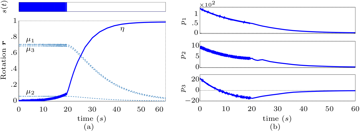
Figure 1: (a) Trajectory of the rotation unit quaternion $\boldsymbol{r}$ in terms of $\eta$ and $\boldsymbol{\mu}$ (dashed line) with switches along time between the discontinuous control laws in (6) represented by $s(t)$. (b) Trajectory of the three-dimensional translation elements $\boldsymbol{p}=p_{1}\hat{\imath}+p_{2}\hat{\jmath}+p_{3}\hat{k}$.

4 Kinematic hybrid control law for robust global pose stability

In this section, we address the control design problem for globally stabilizing a rigid body coupled rotational and translational kinematics with no representation singularities. The proposed solution copes with the topological constraint inherent from the $\text{Spin}(3)\ltimes\mathbb{R}^{3}$ parametrization while also ensuring robustness against measurement noises.

To avoid the unwinding phenomenon and the lack of robustness from pure discontinuous solutions, we appeal to the hybrid system formalism of [34]. This formalism combines both continuous-time and discrete-time dynamics and is useful to formally analyze hysteresis-based control laws, such as the proposed solution. A hybrid system is given by the constrained differential inclusions

$$\begin{split}\dot{x}\in F\left(x\right),&\quad x\in C,\\ x^{+}\in G\left(x\right),&\quad x\in D,\end{split}$$ (7)

where $x^{+}$ denotes the next state of the hybrid system after a jump. The flow map $F$ and the jump map $G$ are set-valued functions, respectively, modeling the continuous and the discrete time dynamics of the system. The flow set $C$ and the jump set $D$ are the respective sets where the evolution occur. The following concepts of set-valued analysis will also be used: a set-valued mapping $F$ is outer semicontinuous if its graph is closed and $F$ is locally bounded—that is, if for any compact set $K$, there exists $m>0$ such that $F\left(K\right)\subset m\mathbb{B}$, where $\mathbb{B}$ is the closed unit ball in the Euclidean space of the convenient dimension [35]. For more details, the reader is referred to [34, 36].

To solve the problem of robust global asymptotic stabilization of (3), we propose a generalization to the hysteresis-based hybrid control law of [11] that extends the attitude stabilization to render both coupled kinematics—attitude and translation—stable. The proposed control law is defined as

$$\underline{\boldsymbol{\omega}}\triangleq-k_{1}h\boldsymbol{\mu}-\varepsilon k_{2}\eta\boldsymbol{\mu}^{\prime},$$ (8)

where $k_{1},k_{2}\in\mathbb{R}_{+}^{*}$ are control gains and $h\in\{-1,1\}$ is a memory state with hysteresis characterized by a parameter $\delta\in\left(0,1\right)$. The memory state $h$ has its dynamics defined by

$$\begin{split}\dot{h}\triangleq 0,&\quad\text{when }\left(\underline{\boldsymbol{q}},h\right)\text{ are such that }h\eta\geq-\delta,\\ h^{+}\in\overline{\operatorname{sgn}}\left(\eta\right),&\quad\text{when }\left(\underline{\boldsymbol{q}},h\right)\text{ are such that }h\eta\leq-\delta,\end{split}$$ (9)

where $\overline{\operatorname{sgn}}$ is the set-valued function defined as

$$\overline{\operatorname{sgn}}\left(s\right)\triangleq\begin{cases}\left\{1\right\},&s>0,\\ \left\{-1\right\},&s<0,\\ \left\{-1,1\right\},&s=0.\end{cases}$$

In terms of the hybrid formalism (7), the closed loop system made by (3), (8) and (9) is characterized as

$$\begin{aligned} F\left(\underline{\boldsymbol{q}},h\right)=\left(\frac{1}{2}\underline{\boldsymbol{q}}\underline{\boldsymbol{\omega}},0\right),C=\left\{\left(\underline{\boldsymbol{q}},h\right)\in\left(\text{Spin}(3)\ltimes\mathbb{R}^{3}\right)\times\{-1,1\}:\ h\eta\geq-\delta\right\},\\ G\left(\underline{\boldsymbol{q}},h\right)\in\left(\underline{\boldsymbol{q}},\overline{\operatorname{sgn}}\left(\eta\right)\right),D=\left\{\left(\underline{\boldsymbol{q}},h\right)\in\left(\text{Spin}(3)\ltimes\mathbb{R}^{3}\right)\times\{-1,1\}:\ h\eta\leq-\delta\right\},\end{aligned}$$ (10)

where $\underline{\boldsymbol{\omega}}$ is defined as in (8) and $h$ as in (9).

Consider $\boldsymbol{\mu}=\hat{\imath}\mu_{1}+\hat{\jmath}\mu_{2}+\hat{k}\mu_{3}$ and $\boldsymbol{\mu^{\prime}}=\hat{\imath}\mu^{\prime}_{1}+\hat{\jmath}\mu^{\prime}_{2}+\hat{k}\mu^{\prime}_{3}$. The map from $\mathbb{H}\otimes\mathbb{D}$ to $\mathbb{R}^{8}$ given by

$$\underline{\boldsymbol{q}}=\eta+\boldsymbol{\mu}+\varepsilon\left(\eta^{\prime}+\boldsymbol{\mu}^{\prime}\right)\mapsto\operatorname{vec}\left(\underline{\boldsymbol{q}}\right)=[\eta,\mu_{1},\mu_{2},\mu_{3},\eta^{\prime},\mu^{\prime}_{1},\mu^{\prime}_{2},\mu^{\prime}_{3}]^{T}$$ (11)

is a vector space isomorphism whose inverse will be denoted by $\underline{\operatorname{vec}}$.

The Hamilton operator [31, 5] provides a matrix representation for the algebraic multiplication through the map $\overset{+}{\operatorname{\boldsymbol{H}}}:\mathbb{H}\otimes\mathbb{D}\rightarrow\mathbb{R}^{8\times 8}$ satisfying

$$\operatorname{vec}\left(\underline{\boldsymbol{q}}_{1}\underline{\boldsymbol{q}}_{2}\right)=\overset{+}{\operatorname{\boldsymbol{H}}}\left(\underline{\boldsymbol{q}}_{1}\right)\operatorname{vec}\left(\underline{\boldsymbol{q}}_{2}\right)$$ (12)

for any $\underline{\boldsymbol{q}}_{1},\underline{\boldsymbol{q}}_{2}\in\mathbb{H}\otimes\mathbb{D}$. Explicitly, the Hamilton operator is given by

$$\underline{\boldsymbol{q}}=\boldsymbol{q}+\varepsilon\boldsymbol{q}^{\prime}\mapsto\overset{+}{\operatorname{\boldsymbol{H}}}\left(\underline{\boldsymbol{q}}\right)=\begin{bmatrix}\overset{+}{\operatorname{\boldsymbol{H}}}_{4}(\boldsymbol{q})&0_{4}\\ \overset{+}{\operatorname{\boldsymbol{H}}}_{4}(\boldsymbol{q}^{\prime})&\overset{+}{\operatorname{\boldsymbol{H}}}_{4}(\boldsymbol{q})\end{bmatrix},$$

where $\overset{+}{\operatorname{\boldsymbol{H}}}_{4}:\mathbb{H}\rightarrow\mathbb{R}^{4\times 4}$ is the map

$$\boldsymbol{q}=\eta+\hat{\imath}\mu_{1}+\hat{\jmath}\mu_{2}+\hat{k}\mu_{3}\mapsto\overset{+}{\operatorname{\boldsymbol{H}}}_{4}(\boldsymbol{q})=\begin{bmatrix}\eta&-\mu_{1}&-\mu_{2}&-\mu_{3}\\ \mu_{1}&\eta&-\mu_{3}&\mu_{2}\\ \mu_{2}&\mu_{3}&\eta&-\mu_{1}\\ \mu_{3}&-\mu_{2}&\mu_{1}&\eta\end{bmatrix}.$$

Let $\boldsymbol{x}=(x_{1},\ldots,x_{8})\in\mathbb{R}^{8}$ and $y\in\mathbb{R}$. Based on (11) and (12), the maps $F$ and $G$ of (10) induce the function $\vec{F}:\mathbb{R}^{9}\rightarrow\mathbb{R}^{9}$ and the set-valued mapping $\vec{G}:\mathbb{R}^{9}\rightrightarrows\mathbb{R}^{9}$ given by

$$\vec{F}(\boldsymbol{x},y)=\left(\frac{1}{2}\overset{+}{\operatorname{\boldsymbol{H}}}\left(\underline{\operatorname{vec}}(\boldsymbol{x})\right)\operatorname{vec}\left(\underline{\boldsymbol{\omega}}\right),0\right),\ \vec{G}(\boldsymbol{x},y)\in\left(\boldsymbol{x},\overline{\operatorname{sgn}}\left(x_{1}\right)\right),$$ (13)

where

$$\operatorname{vec}\left(\underline{\boldsymbol{\omega}}\right)=[0,-k_{1}hx_{2},-k_{1}hx_{3},-k_{1}hx_{4},0,-k_{2}x_{1}x_{6},-k_{2}x_{1}x_{7},-k_{2}x_{1}x_{8}]^{T}.$$

Similarly, the sets $C$ and $D$ of (10) induce the subsets $\vec{C}$ and $\vec{D}$ of $\mathbb{R}^{9}$ given by

$$\begin{split}\vec{C}=\left\{\left(\boldsymbol{x},y\right)\in\mathbb{R}^{8}\times\mathbb{R}:\left(\boldsymbol{x},y\right)\in\underline{\boldsymbol{S}}\times\{-1,1\}\text{ and }yx_{1}\geq-\delta\right\},\\ \vec{D}=\left\{\left(\boldsymbol{x},y\right)\in\mathbb{R}^{8}\times\mathbb{R}:\left(\boldsymbol{x},y\right)\in\underline{\boldsymbol{S}}\times\{-1,1\}\text{ and }yx_{1}\leq-\delta\right\}.\end{split}$$ (14)

The following lemma proves that the hybrid system induced by (3), (8) and (9) satisfies some properties which helps to prove the stability of the system and its robustness.

Lemma 2.

The maps $\vec{F}$ and $\vec{G}$ defined on (13) and the sets $\vec{C}$ and $\vec{D}$ defined on (14) satisfy the following properties:

1. $\vec{C}$ and $\vec{D}$ are closed sets in $\mathbb{R}^{9}$.

2. $\vec{F}:\mathbb{R}^{9}\rightarrow\mathbb{R}^{9}$ is continuous.

3. $\vec{G}:\mathbb{R}^{9}\rightrightarrows\mathbb{R}^{9}$ is an outer semicontinuous set-valued mapping, locally bounded and $\vec{G}\left(\boldsymbol{x},h\right)$ is nonempty for each $\left(\boldsymbol{x},h\right)\in\vec{D}$.

Proof.

The proof is based on Lemma 5.1 of [11]. Setting $\delta\in(0,1)$, consider the continuous map $\tau:\mathbb{R}^{9}\rightarrow\mathbb{R}$ given by $\tau\left(x_{1},\ldots,x_{8},y\right)=yx_{1}+\delta$. The restriction $\tau|_{\underline{\boldsymbol{S}}\times\{-1,1\}}:\underline{\boldsymbol{S}}\times\{-1,1\}\rightarrow\mathbb{R}$ of this map to $\underline{\boldsymbol{S}}\times\{-1,1\}$ is also continuous [37, Theorem 8]. Moreover, by the definition of the sets $\vec{C}$ and $\vec{D}$, we have that

$$\vec{C}=\tau|_{\underline{\boldsymbol{S}}\times\{-1,1\}}^{-1}\left([0,+\infty)\right),$$

$$\vec{D}=\tau|_{\underline{\boldsymbol{S}}\times\{-1,1\}}^{-1}\left((-\infty,0]\right).$$

Since the preimage of a closed set under a continuous mapping is closed, $\vec{C}$ and $\vec{D}$ are closed in $\underline{\boldsymbol{S}}\times\{-1,1\}$. We also have that $\underline{\boldsymbol{S}}\times\{-1,1\}$ is closed in $\mathbb{R}^{9}$. In fact, consider the continuous functions $p,\,d:\mathbb{R}^{8}\rightarrow\mathbb{R}$ given respectively by

$$p(\eta,\mu_{1},\mu_{2},\mu_{3},\eta^{\prime},\mu^{\prime}_{1},\mu^{\prime}_{2},\mu^{\prime}_{3}) = [\eta,\mu_{1},\mu_{2},\mu_{3}][\eta,\mu_{1},\mu_{2},\mu_{3}]^{T}-1,$$

$$d(\eta,\mu_{1},\mu_{2},\mu_{3},\eta^{\prime},\mu^{\prime}_{1},\mu^{\prime}_{2},\mu^{\prime}_{3}) = [\eta,\mu_{1},\mu_{2},\mu_{3}][\eta^{\prime},\mu^{\prime}_{1},\mu^{\prime}_{2},\mu^{\prime}_{3}]^{T}.$$

By the definition of $p$ and $d$, $\underline{\boldsymbol{S}}=p^{-1}(\{0\})\cap d^{-1}(\{0\})$. Since $\{0\}$ is a closed set of $\mathbb{R}$, the sets $p^{-1}(\{0\})$ and $d^{-1}(\{0\})$ are closed and their intersections are closed. Thus, $\underline{\boldsymbol{S}}$ is closed in $\mathbb{R}^{8}$. Moreover, the set $\{-1,1\}$ is closed in $\mathbb{R}$, therefore the Cartesian product $\underline{\boldsymbol{S}}\times\{-1,1\}$ is closed in $\mathbb{R}^{9}$.

Since $\underline{\boldsymbol{S}}\times\{-1,1\}$ is closed in $\mathbb{R}^{9}$, $\vec{C}$ and $\vec{D}$ are also closed in $\mathbb{R}^{9}$. On the account that each component of $\vec{F}$ is a polynomial, the map $\vec{F}$ is continuous.

The graph of the set-valued mapping $\vec{G}$ is given by $\left\{(\boldsymbol{x},y,z):z\in\vec{G}\left(\boldsymbol{x},y\right)\right\}=\mathbb{R}^{8}\times\mathbb{R}\times\mathbb{R}^{8}\times\{-1,1\}$. Since this set is closed, it follows by definition that $\vec{G}$ is outer semicontinuous.

Furthermore, $\vec{G}$ is locally bounded because given any compact set $K$$\subset\mathbb{R}^{9}$, $\vec{G}(K)\subset K\times\{-1,1\}$ and thus $\vec{G}(K)$ is bounded. Finally, by the definition of $\vec{G}$, $\vec{G}(\boldsymbol{x},y)$ is nonempty for every $(\boldsymbol{x},y)\in\vec{D}$. ∎

Theorem 3.

With $\underline{\boldsymbol{\omega}}$ defined as in (8), the equilibrium points of the closed loop system made by (3), (8) and (9) are $\pm 1$ and the set $\left\{\pm 1\right\}$ is asymptotically stable.

Proof.

Using the control law (8)-(9) in (3), the closed-loop system is

$$\begin{split}\dot{\underline{\boldsymbol{q}}}&=\dot{\eta}+\dot{\boldsymbol{\mu}}+\varepsilon\left(\dot{\eta}^{\prime}+\dot{\boldsymbol{\mu}}^{\prime}\right),\>\text{ with }\dot{\eta}=\frac{1}{2}k_{1}h\left\|\boldsymbol{\mu}\right\|^{2},\\ \dot{\boldsymbol{\mu}}&=-\frac{1}{2}\eta k_{1}h\boldsymbol{\mu},\hskip 28.45274pt\dot{\eta}^{\prime}=\frac{1}{2}\left(k_{1}h+k_{2}\eta\right)\boldsymbol{\mu}^{\prime}\cdot\boldsymbol{\mu},\\ \dot{\boldsymbol{\mu}}^{\prime}&=\frac{1}{2}\left[\left(k_{1}h-k_{2}\eta\right)\boldsymbol{\mu}\times\boldsymbol{\mu}^{\prime}-k_{1}h\eta^{\prime}\boldsymbol{\mu}-k_{2}\eta^{2}\boldsymbol{\mu}^{\prime}\right].\end{split}$$ (15)

To find the equilibria of (15), note that $\dot{\underline{\boldsymbol{q}}}=0$ implies $\boldsymbol{\mu}=0.$ From the unit sphere constraint (1), it also follows that $\eta=\pm 1$ whereby we can find that $\boldsymbol{\mu}^{\prime}=0$. In this context, the constraint (5) also renders $\eta^{\prime}=0$. Hence, the set of equilibrium points of (15) is the set $\left\{\pm 1\right\}$.

To study the stability of the set of equilibrium points $\left\{\pm 1\right\}$, let us regard the Lyapunov candidate function

$$V(\underline{\boldsymbol{q}},h)=2\left(1-h\eta\right)+\eta^{\prime 2}+\left\|\boldsymbol{\mu}^{\prime}\right\|^{2}.$$ (16)

Since $\eta\in\left[-1,1\right]$ and $h\in\left\{-1,1\right\}$, one has that $\left(1-h\eta\right)\geq 0.$ Therefore, $V$ is a positive semidefinite function. The condition $V=0$ implies $0\leq 2\left(1-h\eta\right)=-\eta^{\prime 2}-\left\|\boldsymbol{\mu}^{\prime}\right\|^{2}\leq 0$ which yields $\eta^{\prime}=0$, $\boldsymbol{\mu}^{\prime}=0$ and $h\eta=1$, that is, $\underline{\boldsymbol{q}}=\pm 1$. Hence, $V$ is a positive definite function.

Taking the time-derivative of $V$ and using (15) yields

$$\dot{V} =-2h\dot{\eta}+2\eta^{\prime}\dot{\eta}^{\prime}+2\boldsymbol{\mu}^{\prime}\cdot\dot{\boldsymbol{\mu}}^{\prime}$$

$$=-h^{2}k_{1}\left\|\boldsymbol{\mu}\right\|^{2}-\eta^{2}\eta^{\prime 2}k_{2}-\eta^{2}\left\|\boldsymbol{\mu}^{\prime}\right\|^{2}k_{2}\leq 0.$$

In addition, $\dot{V}=0$ if and only if $\underline{\boldsymbol{q}}\in\{\pm 1\}$. Moreover, $V$ also decreases over jumps of the closed loop system since for $h\eta<-\delta<0$ one has that

$$V(\underline{\boldsymbol{q}},h^{+})-V(\underline{\boldsymbol{q}},h)=4h\eta<0.$$

Thus, asymptotically stability of the set $\left\{\pm 1\right\}$ follows from Lemma 2 and by Theorem 20 of [34]. It is also important to highlight that the closed-loop differential equation is well-posed [38, Prop. 2.1] as $\underline{\boldsymbol{\omega}}$ is in the Lie algebra of $\text{Spin}(3)\ltimes\mathbb{R}^{3}$. ∎

Remark 4.

At a first glance, one could imagine that due to the transference principle [25], the extension of rotation stabilizers (e.g., the ones of [39, 11]) to full rigid body stabilizers would be trivial, only requiring the substitution of adequate variables as in (2) and (3). However, for stability analysis based on Lyapunov functions, this supposition doesn’t even make sense, since a Lyapunov function is a real-valued function and never a dual-number valued function. As a consequence, stabilization in $\text{Spin}(3)\ltimes\mathbb{R}^{3}$ using dual quaternions required one independent study from the quaternion stabilization analysis in $\text{Spin}(3)$. The necessity of different procedures for quaternion and dual quaternion is also inferred by remembering that due to the fact that $\textrm{SO}(3)$ is compact and $\textrm{SE}(3)$ is not, it was required one controller design procedure for each case in [3].

Similarly to the rotation controllers proposed in [11], the proposed pose controller doesn’t exhibit Zeno behavior [34]. This is shown in the next lemma.

Lemma 5.

For any compact set $K\subset\underline{\boldsymbol{S}}\times\left\{-1,1\right\}$, if $x$ is a solution of (3), (8) and (9) with initial state in $K$, then the number of jumps is bounded.

Proof.

Similar to Theorem 5.3 of [11]. ∎

The stability robustness will be characterized by the system’s resistance against $\alpha$-perturbations: given $\alpha>0$, the $\alpha$-perturbation of the hybrid system given by $\vec{F},\vec{G}$ as in (13), and $\vec{C},\vec{D}$ as in (14), is given by

$$\vec{C}_{\alpha}\triangleq\left\{x\in\mathbb{R}^{9}:\left(x+\alpha\mathbb{B}\right)\cap\vec{C}\neq\emptyset\right\},$$

$$\vec{F}_{\alpha}\left(x\right)\triangleq\overline{\mathrm{co}}\,\vec{F}\left(\left(x+\alpha\mathbb{B}\right)\cap\vec{C}\right)+\alpha\mathbb{B},\ \text{for all }x\in\vec{C}_{\alpha},$$

$$\vec{D}_{\alpha}\triangleq\left\{x\in\mathbb{R}^{9}:\left(x+\alpha\mathbb{B}\right)\cap\vec{D}\neq\emptyset\right\},$$

$$\vec{G}_{\alpha}\left(x\right)\triangleq\left\{v\in\mathbb{R}^{9}:v\in g+\alpha\mathbb{B},g\in\vec{G}\left((x+\alpha\mathbb{B})\cap\vec{D}\right)\right\},\ \text{for all }x\in\vec{D}_{\alpha},$$

where $\overline{\mathrm{co}}\,X$ denotes the closure of the convex hull of the set $X$. These perturbations, as illustrated in [34], include both measurement and modeling error.

The lack of sensitivity to these perturbations will be expressed in Theorem 6 by bounding the Lyapunov function by a class-$\mathcal{KL}$ function. This bound guarantees practical stability for perturbed solutions starting from arbitrarily large subsets of the basin of attraction of $\{\pm 1\}$ [34].

Theorem 6.

Let $V$ be as in (16). Then there exists a class-$\mathcal{KL}$ function $\beta$ such that for each compact set $K\subset{\underline{\boldsymbol{S}}\times\left\{-1,1\right\}}$ and $\Delta>0$ there exists $\alpha^{*}>0$ such that for each $\alpha\in\left(0,\alpha^{*}\right]$, the solutions $x_{\alpha}$ from $K$ of the perturbed system $\mathcal{H}_{\alpha}=(\vec{C}_{\alpha},\vec{F}_{\alpha},\vec{D}_{\alpha},\vec{G}_{\alpha})$ satisfy

$$V\left(x_{\alpha}\left(t,j\right)\right)\leq\beta\left(V\left(x_{\alpha}\left(0,0\right)\right),t+j\right)+\Delta,\ \forall\left(t,j\right)\in\mathrm{dom}\,x_{\alpha}$$

Proof.

We have that $V$ is a proper indicator function of the compact set $\left\{(1,1),(-1,-1)\right\}$ in ${\underline{\boldsymbol{S}}\times\left\{-1,1\right\}}$. From [34, Theorem 14], there exists a class-$\mathcal{KL}$ function $\beta$ such that for all solutions $x$ of ${\underline{\boldsymbol{S}}\times\left\{-1,1\right\}}$,

$$V\left(x\left(t,j\right)\right)\leq\beta\left(V\left(x\left(0,0\right)\right),t+j\right),\ \forall\left(t,j\right)\in\mathrm{dom}\,x.$$

From this and from Lemma 2, the $\mathcal{KL}$ bound on $V\left(x_{\alpha}\left(t,j\right)\right)$ follows now by [34, Theorem 17]. ∎

Remark 7.

Differently from the Lyapunov function proposed in [11] for its hybrid kinematic controller, the proposed Lyapunov function (16) exploits the non-compactness of $\underline{\boldsymbol{S}}$ to be a proper indicator function, enabling the direct proof of Theorem 6.

5 Numerical simulations

In this section, the effectiveness of the proposed hybrid technique for robust global stabilization of the rigid body motion is demonstrated in four different numerical simulations. The first simulation considers the robustness of the proposed controller against chattering. The second simulation shows the influence of the design parameter $\delta$ in the execution of the controller. The last two simulations consider a more practical situation using a robotic manipulator.

We first illustrate the proposed controller global stability and robustness against measurement noises. To this aim, a simulation is performed using the hybrid feedback controller (8), with hysteresis parameter $\delta=0.3$, and the pure discontinuous controller (6)—using the same proportional gain $k=0.08$. For this particular scenario, we assume an initial condition, $\underline{\boldsymbol{q}}_{0}=0.001+\hat{\imath}0.72+\hat{\jmath}0.06+\hat{k}0.69+\varepsilon\left({-}55.15{-}\hat{\imath}2.52{+}\hat{\jmath}36.71{-}\hat{k}0.59\right)$, which was chosen arbitrarily, located in the neighborhood of $\eta=0$, and a measurement noise over $\eta$ set to $\mathcal{N}(0,0.16)$, that is, a Gaussian random variable with zero mean and $0.16$ variance. Fig. 1 illustrates the result from the discontinuous controller (6) whereby one can clearly see the problematic noise influence—for instance, the excess of switches causing chattering for up to $20$ seconds and the consequent convergence lag. In contrast, the proposed hybrid feedback controller ensures a robust performance without chattering as shown in Fig. 2.

To further highlight the absence of chattering and performance improvements from the hybrid feedback solution (8)—regardless the initial and noise conditions and the control parameters—a second scenario is devised with initial condition $\underline{\boldsymbol{q}}_{0}=0.001+\hat{\imath}0.78+\hat{\jmath}0.57+\hat{k}0.28+\varepsilon\left({-}1.28{+}\hat{\imath}1.50{-}\hat{\jmath}2.44{+}\hat{k}0.77\right)$ and a zero mean Gaussian measurement noise over $\eta$ with a $0.1$ standard deviation, which was also chosen arbitrarily. The results illustrating the trajectory of $\eta$ from both the discontinuous and hybrid controllers—set with the same control gain, $k=2$—are shown in Fig. 3.

(a)	(b)

Figure 2: Numerical example for the hybrid controller: (a) Trajectory of the rotation unit quaternion $\boldsymbol{r}$ in terms of $\eta$ and $\boldsymbol{\mu}$ (dashed line). (b) Trajectory of the three-dimensional translation elements $\boldsymbol{p}=p_{1}\hat{\imath}+p_{2}\hat{\jmath}+p_{3}\hat{k}$.

Figure 3: Trajectory of $\eta$ with hybrid feedback controller (8) and discontinuous controller (6) over time.

To illustrate the influence of the design parameter $\delta$ over the switches along time of the closed-loop system (3), a set of simulations is performed using the hybrid controller (8) with different values for $\delta$. For these simulations, we assume the same initial condition, control gain, and measurement noise as defined in the former scenario. As shown in Fig. 4(a), larger hysteresis parameters yield a smaller number of switches, as one would expect. As shown in Fig. 4(b), it is also interesting to highlight that the number of switches tends to decrease along time as $\eta$ converges to the equilibrium.

(a)	(b)

Figure 4: The number of switches with regard to the hysteresis parameter $\delta$ is shown in (a), while the switches along time $s(t)$ are illustrated in (b) for different values of $\delta$.

Moreover, to elucidate the influence of the hysteresis parameter $\delta$ with regard to the unwinding phenomenon, a different scenario is simulated using (8) with $\delta=0.15$ and $\delta=0.95$ and with a proportional gain $k=5$. We assume an initial state with $\eta$ close to $-1$ and $h=1$. As shown in Fig. 5, very large values of $\delta$ may induce the stabilization to $\eta=1,$ which leads to needless motions and control efforts compared to the case of $\delta=0.15$.

Figure 5: Influence of the hysteresis parameter $\delta$ on unwinding—$\eta$ converges to the farther stable point when the value of $\delta$ increases.

Lastly, as a concluding example, and to assess the effectiveness of the proposed solution in a more practical context, we designed a simple robot manipulator kinematic control task. To this aim, we considered a 6-DOF manipulator, the Comau SMART SiX robot, and two simple control tasks whereby the end-effector of the robot manipulator is regarded as a rigid body and described within the unit dual quaternion framework.

Figure 6: Trajectory of the rotation unit quaternion $\boldsymbol{r}$ in terms of $\eta$ and $\boldsymbol{\mu}$ using the proposed hybrid controller (left), the discontinuous controller (center), and the continuous feedback controller (right). The unwinding phenomenon arises only on the continuous feedback controller.

In the first control setting, the end-effector of the manipulator $\underline{\boldsymbol{q}}_{m}$, described within unit dual quaternions framework, is expected to hold the same current configuration—hence, the desired pose $\underline{\boldsymbol{q}}_{d}=\underline{\boldsymbol{q}}_{m}$—in the presence of different sensor readings. In this case, it is rather ordinary to have readings in the antipodal configuration of the current pose, that is, $-\underline{\boldsymbol{q}}_{m}$. To illustrate the behavior of different controllers—with gain equally set to $k=5$—within this particular case, that is, $\underline{\boldsymbol{q}}_{d}=-\underline{\boldsymbol{q}}_{m}$, we set the manipulator to a random configuration and sought to stabilize the system using a continuous feedback controller, a discontinuous controller, and the proposed hybrid controller (with $\delta=0.1$). The simulated result can be observed in Figs. 6 and 7, which illustrate the rigid motion of the manipulator’s end-effector. Clearly, the continuous feedback controller failed to maintain the same end-effector configuration, exhibiting the unwinding phenomenon which yields needless motions—as observed in Fig. 11. Such phenomena could be avoided by simply enforcing a discontinuous controller or by using the proposed hysteresis-based hybrid control strategy.

Figure 7: Trajectory of the three-dimensional translation error using the hybrid (solid line), the discontinuous (red dashed line) and the continuous controller (magenta dashed line).

Figure 8: Simulation snapshots of the continuous controller, when the desired robot pose, represented by $\underline{\boldsymbol{q}}$, is changed to the same pose, but now represented by $-\underline{\boldsymbol{q}}$. The unwinding phenomenon can be observed in contrast to maintaining the desired pose. In all snapshots, the light red robot represents the initial robot configuration.

Nonetheless, as observed in Fig. 3, the discontinuous sign-based approach is particularly sensitive to measurement noises. Hence, the second control task was devised to illustrate the behavior of the robot manipulator in the presence of measurement noises. In this scenario, both controllers were supposed to take the end-effector pose from an initial pose, represented by $\underline{\boldsymbol{q}}_{0}{=}-0.31-\hat{\imath}0.67+\hat{\jmath}0.67-\hat{k}0.05+\varepsilon\left({-}0.06{-}\hat{\imath}0.31{-}\hat{\jmath}0.31{+}\hat{k}0.40\right)$ and corresponding to a rotation angle of $(\pi+0.63)$ rad around the axis $(-\sqrt{2}/2,-\sqrt{2}/2,0)$ followed by a translation of $(-0.39,-0.29,-1.09)$, to a desired pose, represented by $\underline{\boldsymbol{q}}_{d}{=}\hat{\imath}0.707+\hat{\jmath}0.707+\varepsilon\left(0.28{-}\hat{\imath}0.38{+}\hat{\jmath}0.38{+}\hat{k}0.28\right)$ and corresponding to a rotation angle of $\pi$ rad around the axis $(\sqrt{2}/2,\sqrt{2}/2,0)$ followed by a translation of $(-0.79,0.00,-1.07)$. The error between these poses are represented by the dual quaternion $\underline{\boldsymbol{q}}_{e}=\underline{\boldsymbol{q}}_{m}^{*}\underline{\boldsymbol{q}}_{d}$, where $\underline{\boldsymbol{q}}_{m}$ is the measured dual quaternion. In addition, the measurement noise over $\eta$ was set to $\mathcal{N}(0,0.09)$ and the control gain for both controllers were set to $k=0.020$—the hysteresis parameter was set to $\delta=0.1$. Fig. 9 illustrate the rigid motion of the manipulator’s end-effector and the behavior of both controllers. It is easy to see that the problematic noise influence is restricted to the discontinuous controller—resulting in undesired chattering and delaying the closed-loop convergence. As expected, the proposed hybrid solution ensures robust performance, that is, a trajectory without chattering.

Figure 9: The left figure shows the trajectory of the rotation error in terms of the scalar part $\eta$ using the hybrid (solid line) and the discontinuous controller (red dashed line). The right figure shows the trajectory of the three-dimensional translation elements $\boldsymbol{p}=p_{1}\hat{\imath}+p_{2}\hat{\jmath}+p_{3}\hat{k}$ with reference given in dotted blue line.

6 Conclusion

In this paper, a kinematic controller for the rigid body stabilization problem was presented. To prove the stability of this controller, a Lyapunov function that exploits the structure of the group of unit dual quaternions was proposed. Moreover, this controller was simulated and compared to another kinematic controller based on dual quaternions that has recently been presented in the literature. Simulation results show that the proposed controller is robust against measurement noises and, different from discontinuous-based feedback controllers, it also avoids the problem of sensitivity of the global stabilization property to chattering. The proposed solution was also simulated in a simple robot manipulator kinematic control task to assess the controller in a more practical context.

In other scenarios it is possible that the input to the system is done by torques and forces instead of the generalized velocity. Further work will aim to incorporate the inertial parameters in the controller design.

Appendix

Theorem 8.

[1] Let $\mathcal{M}$ be a manifold of dimension $m$ and consider a continuous vector field $f$ on $\mathcal{M}$. Suppose $\pi:\mathcal{M}\rightarrow\mathcal{L}$ is a vector bundle on $\mathcal{L}$, where $\mathcal{L}$ is a compact, $r$-dimensional manifold with $r\leq m$. Then there exists no equilibrium of $f$ that is globally asymptotically stable.

References

- Bhat and Bernstein [2000] S. P. Bhat, D. S. Bernstein, A topological obstruction to continuous global stabilization of rotational motion and the unwinding phenomenon, Syst. Contr. Letts. 39 (1) (2000) 63–70.
- Aspragathos and Dimitros [1998] N. A. Aspragathos, J. K. Dimitros, A Comparative Study of Three Methods for Robot Kinematics, IEEE Trans. Syst., Man, Cybern. B 28 (2) (1998) 135–145.
- Bullo and Murray [1995] F. Bullo, R. M. Murray, Proportional Derivative (PD) Control on the Euclidean Group, Technical Report Caltech/CDS 95–010, California Institute of Technology, 1995.
- Selig [2007] J. M. Selig, Geometric Fundamentals of Robotics, Monographs in Computer Science, Springer, 2nd edn., 2007.
- Adorno [2011] B. V. Adorno, Two-arm Manipulation: From Manipulators to Enhanced Human-Robot Collaboration, Ph.D. thesis, Laboratoire d’Informatique, de Robotique et de Microélectronique de Montpellier (LIRMM) - Université Montpellier 2, Montpellier, France, 2011.
- Wang and Zhu [2014] X. Wang, H. Zhu, On the Comparisons of Unit Dual Quaternion and Homogeneous Transformation Matrix, Adv. Appl. Clifford Algebras 24 (1) (2014) 213–229.
- Han et al. [2008a] D.-P. Han, Q. Wei, Z.-X. Li, Kinematic control of free rigid bodies using dual quaternions, Int. J. Autom. Comput. 5 (3) (2008a) 319–324.
- Han et al. [2008b] D. Han, Q. Wei, Z. Li, A dual-quaternion method for control of spatial rigid body, in: Proc. 2008 IEEE Int. Conf. Networking, Sensing and Control, 1–6, 2008b.
- Han et al. [2008c] D. Han, Q. Wei, Z. Li, W. Sun, Control of oriented mechanical systems: A method based on dual quaternion, in: Proc. 17th IFAC World Congr., 3836–3841, 2008c.
- Wang and Yu [2013] X. Wang, C. Yu, Unit dual quaternion-based feedback linearization tracking problem for attitude and position dynamics, Syst. Contr. Letts. 62 (3) (2013) 225–233.
- Mayhew et al. [2011] C. G. Mayhew, R. G. Sanfelice, A. R. Teel, Quaternion-based hybrid control for robust global attitude tracking, IEEE Trans. Automat. Contr. 56 (11) (2011) 2555–2566.
- Wang and Yu [2010] X. Wang, C. Yu, Feedback linearization regulator with coupled attitude and translation dynamics based on unit dual quaternion, in: Proc. 2010 IEEE Int. Symp. Intelligent Control, 2380–2384, 2010.
- Wang and Yu [2011] X. Wang, C. Yu, Unit-Dual-Quaternion-Based PID Control Scheme for Rigid-Body Transformation, in: Proc. 18th IFAC World Congr., 9296–9301, 2011.
- Wang et al. [2012a] X. Wang, D. Han, C. Yu, Z. Zheng, The geometric structure of unit dual quaternion with application in kinematic control, J. Math. Anal. Appl. 389 (2) (2012a) 1352–1364.
- Wang et al. [2012b] X. Wang, C. Yu, Z. Lin, A Dual Quaternion Solution to Attitude and Position Control for Rigid-Body Coordination, IEEE Trans. Robot. 28 (5) (2012b) 1162–1170.
- Adorno et al. [2010] B. V. Adorno, P. Fraisse, S. Druon, Dual position control strategies using the cooperative dual task-space framework, in: Proc. 2010 IEEE/RSJ Int. Conf. Intell. Robots Syst., 3955–3960, 2010.
- Pham et al. [2010] H.-L. Pham, V. Perdereau, B. V. Adorno, P. Fraisse, Position and orientation control of robot manipulators using dual quaternion feedback, in: Proc. 2010 IEEE/RSJ Int. Conf. Intell. Robots Syst., 658–663, 2010.
- Figueredo et al. [2013] L. F. C. Figueredo, B. V. Adorno, J. Y. Ishihara, G. A. Borges, Robust kinematic control of manipulator robots using dual quaternion representation, in: Proc. 2013 IEEE Int. Conf. Rob. Autom., 1949–1955, 2013.
- Figueredo et al. [2014] L. F. C. Figueredo, B. V. Adorno, J. Y. Ishihara, G. A. Borges, Switching strategy for flexible task execution using the cooperative dual task-space framework, in: Proc. 2014 IEEE/RSJ Int. Conf. Intell. Robots Syst., 1703–1709, 2014.
- Adorno et al. [2015] B. V. Adorno, a. P. L. Bó, P. Fraisse, Kinematic modeling and control for human-robot cooperation considering different interaction roles, Robotica 33 (2) (2015) 314–331.
- Marinho et al. [2015] M. M. Marinho, L. F. C. Figueredo, B. V. Adorno, A Dual Quaternion Linear-Quadratic Optimal Controller for Trajectory Tracking, in: Proc. 2015 IEEE/RSJ Int. Conf. Intell. Robots Syst., 4047–4052, 2015.
- Filipe and Tsiotras [2013] N. Filipe, P. Tsiotras, Simultaneous position and attitude control without linear and angular velocity feedback using dual quaternions, in: Proc. 2013 Amer. Control Conf., 4808–4813, 2013.
- Filipe and Tsiotras [2014] N. Filipe, P. Tsiotras, Adaptive position and attitude-tracking controller for satellite proximity operations using dual quaternions, J. Guid. Control Dynam. 38 (4) (2014) 566–577.
- Filipe et al. [2015] N. Filipe, M. Kontitsis, P. Tsiotras, Extended Kalman Filter for Spacecraft Pose Estimation Using Dual Quaternions, J. Guid. Control Dynam. 38 (9) (2015) 1625–1641.
- Chevallier [1996] D. P. Chevallier, On the transference principle in kinematics: its various forms and limitations, Mech. Mach. Theory 31 (1) (1996) 57–76.
- Hamilton [1844] W. R. Hamilton, On Quaternions, or on a new System of Imaginaries in Algebra: Copy of a Letter from Sir William R. Hamilton to John T. Graves, Esq. on Quaternions, Philos. Mag. 25 (3) (1844) 489–495.
- Clifford [1873] W. K. Clifford, A preliminary sketch of biquaternions, Proc. London Math. Soc. iv (64/65) (1873) 381–395.
- Study [1891] E. Study, Von den Bewegungen und Umlegungen, Mathematische Annalen 39 (4) (1891) 441–565.
- Wu et al. [2005] Y. Wu, X. Hu, D. Hu, T. Li, J. Lian, Strapdown inertial navigation system algorithms based on dual quaternions, IEEE Trans. Aerosp. Electron. Syst. 41 (1) (2005) 110–132.
- Chou [1992] J. C. K. Chou, Quaternion kinematic and dynamic differential equations, IEEE Trans. Robot. Automat. 8 (1) (1992) 53–64.
- McCarthy [1990] J. M. McCarthy, Introduction to Theoretical Kinematics, MIT Press, 1990.
- Lee [2013] J. M. Lee, Introduction to Smooth Manifolds, Springer, 2013.
- Sanfelice et al. [2006] R. G. Sanfelice, M. J. Messina, S. Emre Tuna, A. R. Teel, Robust hybrid controllers for continuous-time systems with applications to obstacle avoidance and regulation to disconnected set of points, in: Proc. 2006 Amer. Control Conf., 3352–3357, 2006.
- Goebel et al. [2009] R. Goebel, R. G. Sanfelice, A. R. Teel, Hybrid Dynamical Systems, IEEE Control Systems 29 (2) (2009) 28–93.
- Rockafellar and Wets [2004] R. T. Rockafellar, R. J.-B. Wets, Variational analysis, Springer, 2 edn., 2004.
- Goebel et al. [2012] R. Goebel, R. G. Sanfelice, A. R. Teel, Hybrid Dynamical Systems: modeling, stability, and robustness, Princeton University Press, 2012.
- Basener [2013] W. Basener, Topology and Its Applications, Pure and Applied Mathematics: A Wiley Series of Texts, Monographs and Tracts, Wiley, 2013.
- Sachkov [2009] Y. L. Sachkov, Control theory on Lie groups, J. Math. Sci 156 (3) (2009) 381–439.
- Bullo et al. [1995] F. Bullo, R. M. Murray, A. Sarti, Control on the Sphere and Reduced Attitude Stabilization, Technical Report Caltech/CDS 95–005, California Institute of Technology, 1995.