LocDyn: Robust Distributed Localization for Mobile Underwater Networks

Abstract

How to self-localize large teams of underwater nodes using only noisy range measurements? How to do it in a distributed way, and incorporating dynamics into the problem? How to reject outliers and produce trustworthy position estimates? The stringent acoustic communication channel and the accuracy needs of our geophysical survey application demand faster and more accurate localization methods. We approach dynamic localization as a MAP estimation problem where the prior encodes dynamics, and we devise a convex relaxation method that takes advantage of previous estimates at each measurement acquisition step; The algorithm converges at an optimal rate for first order methods. LocDyn is distributed: there is no fusion center responsible for processing acquired data and the same simple computations are performed for each node. LocDyn is accurate: experiments attest to a smaller positioning error than a comparable Kalman filter. LocDyn is robust: it rejects outlier noise, while the comparing methods succumb in terms of positioning error.

I Introduction

The development of networked systems of agents that can interact with the physical world and carry out complex tasks in various contexts is currently a major driver for research and technological development [1]. This trend is also seen in contemporary ocean applications and propelled research projects on multi-vehicle systems like MORPH (Kalwa et al. [2]) and, recently, WiMUST (Al-Khatib et al. [3]).

Coordinated operation of vehicles requires a communication network to share data, most critically, those data related to navigation and positioning, as further explored in Abreu et al. [4]. Our work concerns localization of (underwater) vehicles, a key subsystem needed in the absence of GPS to properly georeference any acquired data and also used in cooperative control algorithms. This paper presents research results within the scope of EU H2020 project WiMUST, aiming at advanced control, communication and signal processing tools to enable a team of marine robots, either on the surface or submerged, to jointly conduct geoacoustic surveys.

Today, geophysicists reveal sub-bottom structures using powerful sound sources and hydrophones. During surveys, a towed source produces acoustic waves that penetrate the sea bottom, and its layers are inferred from the pattern of echoes observed at the towed hydrophones, over a long period of time and a wide geographic area. Such surveys are routinely carried out to characterize the sea bottom prior to underwater construction, to monitor pipelines and submerged structures, and for the operation of offshore oil and gas fields.

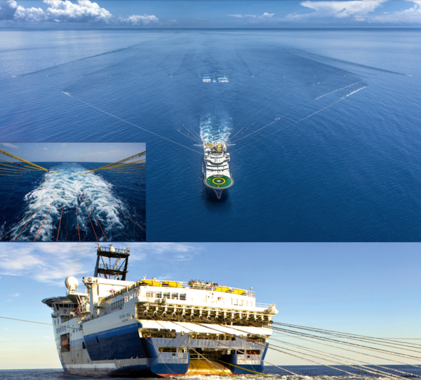
Figure 1: A surface vessel tows streamers with acoustic receivers for geophysical surveys (Al-Khatib et al. [3]).

As depicted in Figure 1, a single vessel tows very long arrays of streamers and, thus, operation of a traditional geophysical survey at sea means we cannot change trajectories to recheck interesting findings; also, maneuvering between rectilinear transects while keeping the streamers untangled is challenging. The vision of WiMUST is to replace the monolithic setup with a more flexible one where multiple heterogeneous underwater vehicles tow smaller arrays while retaining a precise spatial alignment. These are easier to maneuver, and the absence of long physical ties between the surface ship and the data acquisition devices enables new capabilities such as operating at variable depths or adaptively changing the shape of the ensemble of hydrophones.

Self-localization is a cornerstone for multi-vehicle cooperative control in general and for WiMUST in particular, as the acoustic signals must be georeferenced to high precision to enable an accurate inference of deep sub-bottom layers. Our specific goal in this paper is to accurately localize a network of moving agents from noisy inter-vehicle ranges and from the positions of a few anchors or landmarks.

Related work

The signal processing and control communities studied the network localization problem in many variants, like static or dynamic network localization, centralized or distributed computations, maximum-likelihood methods, approximation algorithms, or outlier robust methods.

The control community’s mainstream approach to localization relies on the robust and strong properties of the Kalman filter to dynamically compensate noise and bias. Recent approaches can be found in Pinheiro et al. [5] and Rad et al. [6]. In the first very recent paper, position and velocity are estimated from ranges, accelerometer readings and gyroscope measurements with an Extended Kalman filter. The authors of the second paper linearize the dynamic network localization problem, solving it with a linear Kalman filter. This last method is comparable with our range-only problem, although the method requires knowledge of the noise’s standard deviation.

The signal processing community traditionally studies static network localization from a centralized perspective, like Keller and Gur [7], that formulate the problem as a regression over adaptive bases; but the authors use squared distances, prone to outlier noise amplification. Shang et al. [8] follow a multidimensional scaling approach, but multidimensional scaling works well only in networks with high connectivity — a property not encountered in practice in large-scale geometric networks. Biswas et al. [9] and more recently Oğuz-Ekim et al. [10] proposed semi-definite and second order cone relaxations of the maximum likelihood estimator. Although more precise, these convexified problems get intractable even for a small number of nodes. Recently, we have witnessed increasing interest from signal processing in distributed static network localization. Papers by Shi et al. [11], Srirangarajan et al. [12], Chan and So [13], Khan et al. [14], Simonetto and Leus [15] and recently Soares et al. [16] use different convex approximations to the nonconvex optimization costs to devise scalable and distributed algorithms for network localization. But for scenarios where approximate solutions are not enough, researchers optimized the maximum likelihood directly, obtaining solutions that depend on the initialization of the algorithm. The methods in Calafiore et al. [17] and Soares et al. [18] increase the precision of a relaxation-based solution, but are prone to local minima if wrongly initialized. Lately, signal processing researchers produced solutions for dynamic network localization; Schlupkothen et al. [19] incorporated velocity information from past position estimates to bias the solution of a static localization problem via a regularization term.

Our approach

In this paper we deal with the network localization problem from an optimization-based standpoint. We formalize the network localization problem under the maximum a posteriori framework considering white Gaussian noise and we tightly relax the nonconvex estimator to a convex unconstrained program. We optimize the approximated problem with a scalable and fast first order method, achieving smooth trajectories for a small number of distributed iterations. We define distributed operation as requiring no central or fusion node, and where all nodes perform the same types of computations. Distributed operation of vehicles requires the existence of a communication network to share navigation and positioning data.

We propose a distributed algorithm for network localization of underwater mobile nodes with the main properties of following a principled maximum a posteriori approach, distributed iterations at each agent, robustness to outlier measurements, and fast convergence. We call our algorithm localization under dynamics, or LocDyn for short.

While LocDyn supports distributed operation in the classic sense, it may also be viewed in a more restricted way simply as an efficient parallel algorithm when run at a central location that collects all required range measurements through an appropriate forwarding protocol (discussed, e.g., in Ludovico et al. [20]). Depending on the capacity of the shared transmission medium the latter solution may be preferable from a practical standpoint, but it does not impact the derivations below.

Our approach is most closely related to one-shot network localization methods in signal processing (i.e., starting anew when repeated over time), but it adds a temporal dimension that enables filtering to regularize position estimates and thus improve their accuracy. Contrary to many Kalman-filtering-based approaches to localization in the control literature, we assume an extremely simple dynamic model for mobile nodes and do not rely on navigation information that could be provided by an inertial measurement unit (IMU). The rationale for this is that mobile nodes in our scenarios are not necessarily AUVs; provisions could be made to install some range-measurement and communication devices in streamers, whose dynamics are not as well characterized as those of the towing AUVs, and where the presence of high-quality IMUs seems far-fetched at present.

I-A Contributions

We introduce LocDyn, the first optimization-based dynamic network localization estimator that is fully distributed and has optimal convergence rate. LocDyn tightly approximates the MAP estimator, with the nodes’ dynamics as priors, so Bayesian estimation properties are to be expected. We use a position predictor with information from previous position estimates via a low-pass velocity approximation. Our method is more accurate than a Kalman filter implementation by more than 30cm per trajectory point in all our experiments.

In our companion UCOMMS’16 paper (Ferreira et al. [21]) we focused on demonstrating benefits for collaborative localization using hybrid range/bearing measurements and time-domain filtering. We explore the same fundamental idea for time-recursive processing here, but the method for predicting velocities is now considerably improved, and we propose an efficient distributed localization algorithm, whereas in Ferreira et al. the dynamic optimization problem was solved using a general-purpose (centralized) convex solver. Also, the algorithm is carefully characterized and benchmarked using numeric simulations.

The hybrid setup of Ferreira et al. adopts the FLORIS/CLORIS least-squares framework (from a previous work by Ferreira et al. [22]), which in turn relies on a so-called disk-based relaxation presented in Soares at al. [16] to attain a high-precision convex formulation that is amenable to distributed/parallel processing. In the present paper we consider exclusively range measurements to streamline the technical content, but we emphasize that accommodating bearing measurements in a hybrid localization scheme involves only minor adaptations in the optimization problem and distributed solution algorithm.

II Static network localization

The network of range-measurement and communication devices (nodes), installed on AUVs and conceivably on streamers as well, is represented as an undirected connected graph $\mathcal{G}=(\mathcal{V},\mathcal{E})$. The node set $\mathcal{V}=\{1,2,\dots,n\}$ denotes the agents with unknown positions. There is an edge $i\sim j\in{\mathcal{E}}$ between $i$ and $j$ if a noisy range measurement between nodes $i$ and $j$ is available at both, and if $i$ and $j$ can communicate with each other. The set of landmarks with known positions, named anchors, is denoted by ${\mathcal{A}}=\{1,\ldots,m\}$. For each $i\in{\mathcal{V}}$, we let ${\mathcal{A}}_{i}\subset{\mathcal{A}}$ be the subset of anchors (if any) relative to which node $i$ also possesses a noisy range measurement.

Let ${\mathbb{R}}^{p}$ be the space of interest ($p=2$ for planar networks, and $p=3$ in the volumetric scenarios of greater interest here), $x_{i}\in{\mathbb{R}}^{p}$ the position of sensor $i$, and $d_{ij}$ the noisy range measurement between sensors $i$ and $j$, known by both $i$ and $j$. Without loss of generality, we assume $d_{ij}=d_{ji}$. Anchor positions are denoted by $a_{k}\in{\mathbb{R}}^{p}$. Similarly, $r_{ik}$ is the noisy range measurement between sensor $i$ and anchor $k$, available at sensor $i$.

The distributed network localization problem addressed in this work consists in estimating the sensors’ positions $x=\{x_{i}\,:\,i\in\mathcal{V}\}$, from the available measurements $\{d_{ij}\,:\,i\sim j\}\cup\{r_{ik}\,:\,i\in{\mathcal{V}},k\in{\mathcal{A}}_{i}\}$, through collaborative message passing between neighboring agents in the communication graph ${\mathcal{G}}$.

Under the assumption of zero-mean, independent and identically-distributed, additive Gaussian measurement noise, the maximum-likelihood estimator for the nodes’ positions is the solution of the optimization problem

$$\operatornamewithlimits{minimize}_{x}f(x),$$ (1)

where

$$f(x)=\sum_{i\sim j}\frac{1}{2}(\|x_{i}-x_{j}\|-d_{ij})^{2}+\sum_{i}\sum_{k\in\mathcal{A}_{i}}\frac{1}{2}(\|x_{i}-a_{k}\|-r_{ik})^{2}.$$

Problem (1) is nonconvex and difficult to solve. Even in the centralized setting (i.e., all measurements are available at a central node) currently available iterative techniques don’t claim convergence to the global optimum. Also, even with noiseless measurements, multiple solutions might exist due to ambiguities in the network topology itself [23].

We can address this problem by optimizing a convex approximation to (1), amenable to distributed implementation, as in Soares et al. [16]. The convex approximation $\hat{f}$ is tight at each term of $f$ and can be optimized by a first order method with optimal convergence rate. The approximated problem is

$$\operatornamewithlimits{minimize}_{x}\hat{f}(x).$$ (2)

The convex surrogate function $\hat{f}$ is defined as

$$\hat{f}(x)=\sum_{i\sim j}\frac{1}{2}\mathrm{d}^{2}_{B_{ij}}(x_{i}-x_{j})+\sum_{i}\sum_{k\in\mathcal{A}_{i}}\frac{1}{2}\mathrm{d}^{2}_{Ba_{ik}}(x_{i}),$$ (3)

where $\mathrm{d}^{2}_{B_{ij}}$ and $\mathrm{d}^{2}_{Ba_{ik}}$ are the squared distances to a ball $B_{ij}=\{y:\|y\|\leq d_{ij}\}$, and a ball $Ba_{ik}=\{y:\|y-a_{k}\|\leq r_{ik}\}$, respectively. The convexification strategy underlying (3) is to relax spheres in the constraint sets of squared distance functions to balls (disks) $B_{ij}$, $Ba_{ik}$, hence the name disk-based relaxation. In the next section we will use function $\hat{f}$ and a modified version of problem (2) to localize underwater moving nodes.

II-A Assumptions

Range-only position estimation needs at least $p+1$ anchors, or an equivalent set of physical constraints, to avoid spatial ambiguities [23].

Consequently, all range-only methods assume that the number of anchors, or landmarks, is greater than the dimension of the deployment space — 3 anchors for planar deployment and 4 for a volumetric one.

III Motion-aware localization

One naive approach to localize a network of moving agents would be to estimate the vehicles’ positions solving (2) at each time step. Although it is possible, it does not take advantage of the knowledge of previously estimated positions, so something will be lost in processing time or communication bandwidth.

To bring motion into play we invoke the concept of prior knowledge in Bayesian statistics and assume a Gaussian prior on the nodes’ positions, now understood as random variables. Each position’s distribution depends on the Gaussian distribution of the noisy range measurements, its own prior and distributions of neighboring nodes’ positions. The prior is the predicted position

$$\tilde{x}_{i}(k+1)=\hat{x}_{i}(k)+v(k)_{i}\Delta T,$$ (4)

where $\hat{x}_{i}(k)$ is the estimated position at time step $k$, and $v_{i}(k)$ is the measured or estimated velocity of $i$. As measurements are not taken continuously, we model time in discrete steps $t=k\Delta T$, where $t$ is continuous time, $k$ is the time step, and $\Delta T$ is the sampling period. Without loss of generality we consider $\Delta T$ fixed. The distance measurement between vehicles $i$ and $j$ at positions $x_{i}^{\star}$ and $x_{j}^{\star}$ is modeled as

$$d_{ij}=\|x_{i}^{\star}-x_{j}^{\star}\|+\mathcal{N}(0,\sigma^{2}),$$ (5)

and, similarly, the range measurement between vehicle $i$ and anchor $k$ is

$$r_{ik}=\|x_{i}^{\star}-a_{k}\|+\mathcal{N}(0,\sigma^{2}).$$ (6)

For each node $i$ the prior distribution is also Gaussian, centered on $\tilde{x}_{i}$ with variance $\varsigma^{2}$. Assuming independency, the posterior distribution of the positions at a given time step is, up to a normalization constant, $p(x|\{d\})\propto p(\{d\}|x)p(x)$. This evaluates to

$$\begin{array}[t]{rcl}p(x|\{d\})&\propto&\prod_{i\sim j}p(\|x_{i}-x_{j}\|-d_{ij})\\ &&\prod_{i}\left(\prod_{k\in\mathcal{A}}p(\|x_{i}-a_{k}\|-r_{ik})p(x_{i}-\tilde{x}_{i})\right),\end{array}$$

where all densities on the right-hand side are Gaussian. We cast network localization as a maximum a posteriori estimation problem. After applying the logarithm, we get

$$\operatornamewithlimits{minimize}_{x}\frac{1}{\sigma^{2}}f(x)+\frac{1}{\varsigma^{2}}\sum_{i}\|x_{i}-\tilde{x}_{i}\|^{2},$$ (7)

equivalently written as

$$\operatornamewithlimits{minimize}_{x}f(x)+\lambda\|x-(\hat{x}+v\Delta T)\|^{2},$$

where we multiplied by $\sigma^{2}$ and adopted $\lambda=\frac{\sigma^{2}}{\varsigma^{2}}$. Thus, the parameter $\lambda$ has a physical interpretation: it is the ratio of the uncertainty in the measurements to the richness of the trajectory. The concatenated vehicles’ velocities at time $k$, $v(k)$, can be measured or approximated from the previous location estimates. As we have seen, this problem is nonconvex, so we convexify it using the approach from section II to obtain the problem

$$\operatornamewithlimits{minimize}_{x}g_{\lambda}(x)=\hat{f}(x)+\lambda\|x-(\hat{x}+v\Delta T)\|^{2}.$$ (8)

We can also interpret (8) as a regularized network localization problem. The regularization parameter $\lambda$ controls how much we want to bias our estimate towards the predicted position.

Figure 2: Localization of a moving vehicle: at time $k=2$ our formulation uses velocity information from the previous estimates and biases the estimator in (8) towards the dotted position.

For example, if a node moves linearly as in Figure 2, at $k=2$ our formulation will use velocity $v(1)$ to predict the position of the vehicle, and bias the static localization problem towards the predicted solution.

We introduced problem (8) in Ferreira et al. [21] in the context of hybrid collaborative localization based on range and bearing measurements.

IV The LocDyn algorithm

Problem (8) has properties that allow fast optimization: it is a sum of convex functions and, thus, convex. It is actually strongly convex, meaning that at any point $x$ the function is lower bounded by a quadratic and thus possesses a unique minimum on compact sets (c.f. Boyd and Vandenberghe [24]). Also, our objective function in (8) is L-smooth, meaning that there is a quadratic upper bound to $g_{\lambda}(x)$ for all $x$, so $g_{\lambda}$ does not grow too fast. Appendix A holds proofs and computation of the $L$ and $m$ constants. If $g_{\lambda}$ is strongly convex and has a Lipschitz continuous gradient, a first-order minimization algorithm can be maximally accelerated (c.f. Nesterov [25]).

The gradient of $g_{\lambda}$ is

$$\nabla g_{\lambda}=\nabla\hat{f}(x)+2\lambda(x-\tilde{x}),$$ (9)

where $\nabla\hat{f}$ is, as defined in (15) of Soares et al. [16]:

$$\nabla\hat{f}(x)=\mathcal{L}x-A^{\top}\mathrm{P_{B}}(Ax)+\begin{bmatrix}\sum_{k\in\mathcal{A}_{1}}x_{1}-\mathrm{P_{Ba}}_{1k}(x_{1})\\ \vdots\\ \sum_{k\in\mathcal{A}_{n}}x_{n}-\mathrm{P_{Ba}}_{nk}(x_{n})\end{bmatrix},$$ (10)

where $A=C\otimes I_{p}$, $C$ is the arc-node incidence matrix of $\mathcal{G}$, $I_{p}$ is the identity matrix of size $p$, and $\mathrm{B}$ is the Cartesian product of the balls $\mathrm{B}_{ij}=\{y:\|y\|\leq d_{ij}\}$ corresponding to all the edges in $\mathcal{E}$. Similarly, $\mathrm{Ba}_{ik}=\{y:\|y-a_{k}\|\leq r_{ik}\}$. Also, $\mathcal{L}=A^{\top}A=L\otimes I_{p}$, with $L$ being the Laplacian matrix of graph $\mathcal{G}$.

Algorithm 1 LocDyn

0:  $\begin{array}[t]{l}L;\\ \{d_{ij}(k):i\sim j\in\mathcal{E}\};\\ \{r_{ik}(k):i\in\mathcal{V},k\in\mathcal{A}\};\\ \beta=\frac{1-\sqrt{m/L}}{1+\sqrt{m/L}};\\ \end{array}$

0:  $\hat{x}(k)$

1:  measure or estimate (via (12)) $v_{i}(k-1)\Delta T$

2:  $\tilde{x}_{i}=\hat{x}_{i}(k-1)+v_{i}(k-1)\Delta T$;

3:  $\kappa=0;$

4:  each node $i$ chooses random $x_{i}(0)=x_{i}(-1)$;

5:  while some stopping criterion is not met, each node $i$ do

6:     $\kappa=\kappa+1$

7:     $\begin{aligned} w_{i}=x_{i}(\kappa-1)+\beta\left(x_{i}(\kappa-1)-x_{i}(\kappa-2)\right);\end{aligned}$

8:     node $i$ broadcasts $w_{i}$ to its neighbors

9:     $\begin{array}[]{l}\nabla g_{\lambda i}(w_{i})=\delta_{i}w_{i}-\sum_{j\in N_{i}}w_{j}+\\ +\sum_{j\in N_{i}}c_{(i\sim j,i)}\mathrm{P_{B}}_{ij}(w_{i}-w_{j})+2\lambda(w_{i}-\tilde{x}_{i});\end{array}$

10:     $\begin{aligned} x_{i}(\kappa)=w_{i}-\frac{1}{L}\nabla g_{\lambda i}(w_{i});\end{aligned}$

11:  end while

12:  return  $\hat{x}(k)=x(\kappa)$

Algorithm 1 specifies LocDyn as detailed this far, with its regularization term. As discussed previously, $k$ indexes time steps where we have range data and anchor positions acquisition. in the interval, we run the algorithm, whose steps are indexed by $\kappa$. The procedure inherits and concurs with the distributed properties of the static method in Soares et al. [16]. Step 7 computes the extrapolated points $w_{i}$ in a standard application of Nesterov’s method [26]. Step 9 corresponds to the $i$-th entry of $\nabla\hat{f}$ and an affine term on $x_{i}$ dependent only on each node’s unknown coordinates, velocity, and the position estimated in the previous time step. Constants $c_{(i\sim j,i)}$ denote the entry $(i\sim j,i)$ in the arc-node incidence matrix $C$, and $\delta_{i}$ is the degree of node $i$. The $i$-th entry of $\mathcal{L}x$ can be computed by node $i$ from its current position estimate and the position estimates of the neighbors, as $(\mathcal{L}x)_{i}=\delta_{i}x_{i}-\sum_{j\in N_{i}}x_{j}$. As further detailed in Soares et al. [16],

$$(A^{\top}\mathrm{P_{B}}(Ax))_{i}=\sum_{j\in N_{i}}c_{(i\sim j,i)}\mathrm{P_{B}}_{ij}(x_{i}-x_{j}),$$

as presented in Step 9.

Next, we deal with how to approximate the velocity of a node in the global reference frame only with data collected so far.

IV-A Velocity estimation

To include vehicle dynamics in network localization, we penalize discrepancies between the predicted and estimated positions. The predicted positions are computed based on the previous estimated position and the vehicle’s velocity in world coordinates. This velocity can be measured by the AUV, or, as we consider next, it can be estimated from the moving pattern so far. In a previous paper (Ferreira et al. [21]), inspired by the recent work by Schlupkothen et al. [19], we estimated the velocity of each vehicle in the global reference frame by averaging the norm and the angle over a sliding time window. But prediction by averaging is accurate only if the averaged quantities are nearly constant through time — meaning linear constant motion. This is not necessarily the case in the projected futuristic scenarios for geoacoustic surveying; in this type of application, richer trajectories such as the one depicted in Figure 3(c) are meant to densely cover the geographic area under study. In this paper we estimate each vehicle’s velocity $\hat{v}_{i}$ by taking Taylor expansions of the derivative of the position. We start by approximating velocity by central finite differences. Unlike the causal backward Euler difference approximation, that converges linearly, the centered difference approximation converges quadratically as $\Delta T\to 0$ and is defined as:

$$\hat{v}_{i}(k)\Delta T=\frac{x_{i}(k+1)-x_{i}(k-1)}{2}.$$

Higher order approximations have even faster convergence rates, and they are more robust to noise in the position estimates. Nevertheless, to use them in causal estimators like LocDyn, we have to introduce a time lag that covers the higher order time shifts. As communication in the underwater acoustic channel has low bandwidth and slow propagation speed, networking protocols may entail considerable latency that invalidates the estimation of velocities with too large time shifts, so there is a tradeoff between accuracy and opportunity in choosing the order of approximation. A causal sixth-order approximation is

$$\begin{array}[t]{rcl}\hat{v}_{i}(k)\Delta T&=&\frac{45(x_{i}(k-3)-x_{i}(k-5))}{60}+\\ &&-\frac{9(x_{i}(k-2)-x_{i}(k-6))}{60}+\\ &&\frac{x_{i}(k-1)-x_{i}(k-7)}{60}.\end{array}$$ (11)

However, computing differences amplifies noise. To reduce the impact of noise in velocity estimation, we take the derivative approximation as an anti-symmetric FIR filter with a defined accuracy order. The derivative approximation’s transfer function can then be designed to match the transfer function of the continuous derivative operator. Holoborodko [27] proposed a method to generate differentiator filters that also cut high frequencies, rejecting noise both in measurements and in the estimation process, while preserving the differentiation behavior at low frequencies. This method was successfully used, for example, by Khong et al. [28] or Hosseini and Plataniotis [29]. We use the smooth low noise differentiator fitted from a second-degree polynomial with a lag of 7 samples. Although it takes the same estimates as (11), the low-pass designed coefficients reject high-frequency noise. The expression for the product between estimated velocity and sampling is

$$\begin{array}[]{lcl}\hat{v}_{i}(k)\Delta T&=&\frac{5(x_{i}(k-3)-x_{i}(k-5))}{32}+\\ &&\frac{4(x_{i}(k-2)-x_{i}(k-6))}{32}+\\ &&\frac{x_{i}(k-1)-x_{i}(k-7)}{32}.\end{array}$$ (12)

IV-B Convergence

The accelerated gradient method implemented in Alg. 1 for function $g_{\lambda}$ with constants $m$ and $L$ specified in (14) and (13) converges at the optimal rate $O\left(\kappa^{-2}\right)$ as proved by Nesterov [30],[25]. Also, the distance to the unique global optimum $g_{\lambda}^{\star}$ at iteration $\kappa$ is theoretically bounded by

$$\begin{array}[t]{l}g_{\lambda}(x(\kappa))-g_{\lambda}^{\star}\leq\\ \frac{4}{(2+\kappa\sqrt{m/L})^{2}}\left(g_{\lambda}(x(0))-g_{\lambda}^{\star}+\frac{m}{2}\left\|x(0)-x^{\star}\right\|^{2}\right).\end{array}$$

V Numerical evaluation

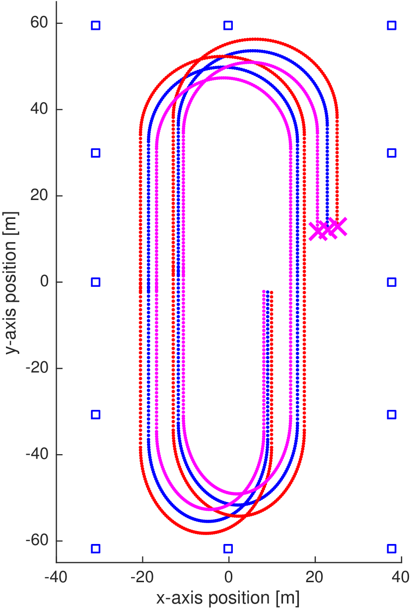
(a) Lap trajectory, with three vehicles (distances in meters).

(b) Descending spiral.

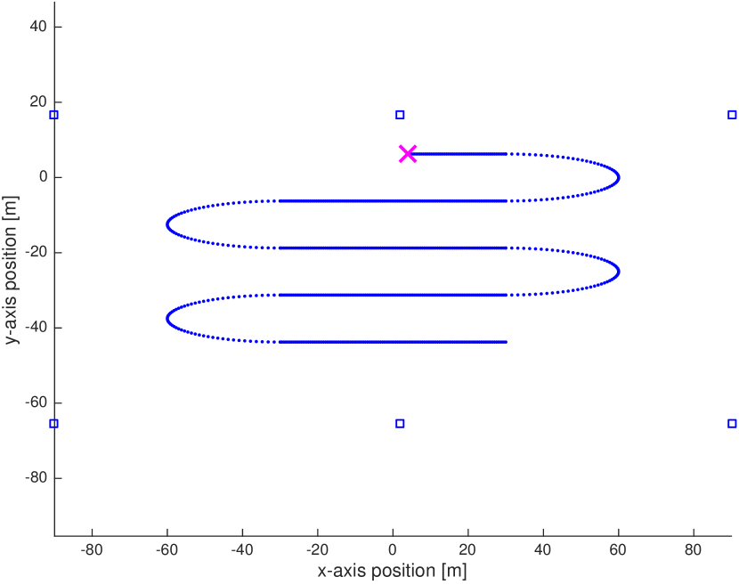
(c) The lawn mower trajectory.

Figure 3: Trajectories for experimental evaluation. The starting position is marked with a magenta cross. Anchors are depicted as blue squares.

We evaluate LocDyn in trajectories used in (not necessarily geoacoustic) surveys: a lap (Figure 3(a)), descending 3D spiral (Figure 3(b)), and the lawn mower (Figure 3(c)).

In all experiments, we contaminate distance measurements at each time step $k$ with zero-mean white Gaussian noise with standard deviation  $\sigma=1$m. This value for the standard deviation of measurement noise is an upper bound on the real-world noise observed in the WiMUST vehicles, where ranging errors are less than 1m. We generated synthetic data according to

$$d_{ij}=|\|x_{i}^{\star}-x_{j}^{\star}\|+\mathcal{N}(0,\sigma^{2})|,$$

for inter-sensor distances and

$$r_{ik}=|\|x_{i}^{\star}-a_{k}\|+\mathcal{N}(0,\sigma^{2})|,$$

for sensor-anchor distances. We emphasize that measurements are in mismatch with the data model considered in Sections II and III, but the discrepancy is not serious, as the likelihood of $d_{ij}$, $r_{ik}$ being nonpositive in (5) and (6) is typically very small.

We benchmark LocDyn against static localization in Soares et al. [16] and against the linear Kalman filter solution proposed by Rad et al. [6]. We compare LocDyn with the Kalman filter in the lap and the lawn mower trajectories and not in the spiral, because the implementation that the authors kindly made available to us works only in 2D. We provided the true $\sigma$ to the Kalman filter, whereas LocDyn and static localization do not use it. All the other Kalman filter parameters were not altered.

We ran 100 Monte Carlo trials for each experiment, and measured the empirical error as

$$\mathrm{Error}=\frac{1}{K}\sum_{k=1}^{K}\|\hat{x}(k)-x^{\star}(k)\|,$$

where $K$ is the total number of steps in the trajectory, and $x^{\star}(k)$ is the concatenation of the true positions $x_{i}^{\star}$. We initialize LocDyn and the Kalman filter in the position marked with a magenta cross. Static localization doesn’t require initialization. Anchors are placed to contain the trajectory on their convex hull. In 2d, we placed 6 anchors for the lawn mower and 12 for the lap. For 3D, we used 16 anchors.

V-A Lap trajectory

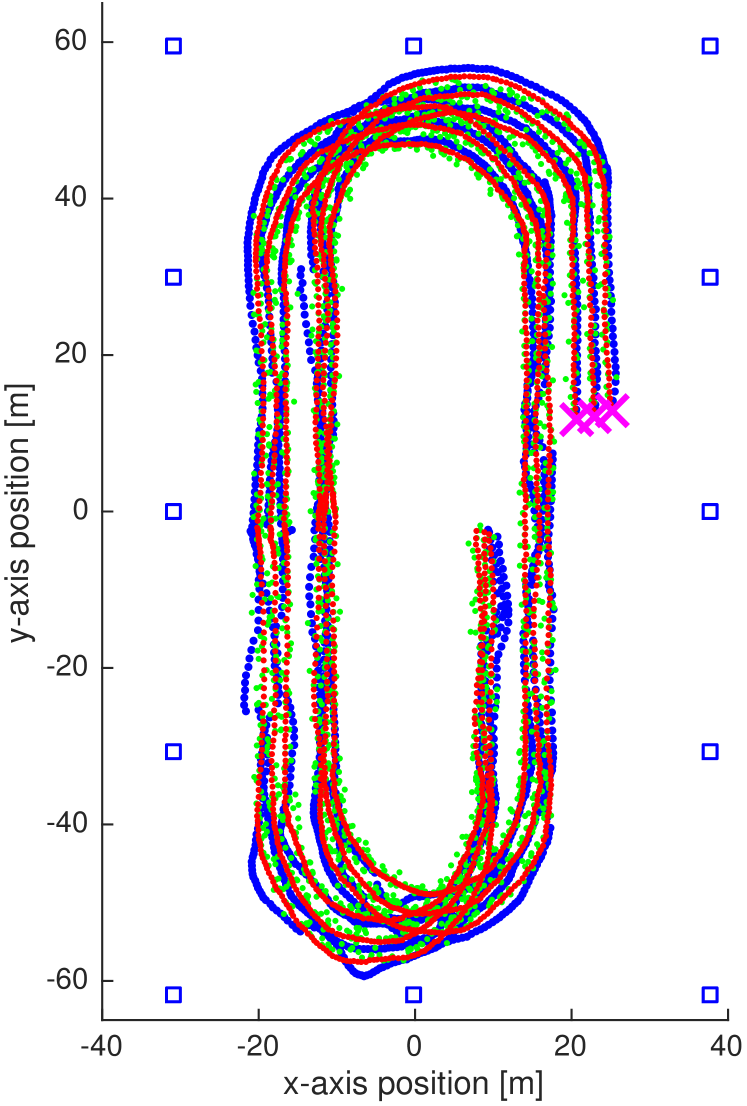
Figure 4: Example run: A team of three underwater vehicles describes a planar lap surveying trajectory. In green, we have the static localization estimates, in blue the Kalman filter, and in red, LocDyn. LocDyn describes the smoothest trajectory. There is a slowdown around (-15,-5) where the Kalman Filter gets lost, maybe due to the assumption of constant velocity.

Lap trajectories are frequent in ocean surveying. They are also rich since they combine linear parts with curved ones. We tested LocDyn, the Kalman filter and static localization in the lap shown in Figure 3(a) and one of the Monte Carlo runs is depicted in Figure 4. We perceive the LocDyn trajectory as the most natural of the three. There is an intentional slowdown of the vehicles around (-15,-5) and LocDyn is the least affected by it. We observed these behaviors in all our visualizations of the lap estimated trajectories.

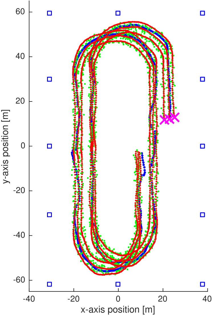
Figure 5: Example run: A team of three underwater vehicles describes a planar lap surveying trajectory. For the Kalman filter estimates, we display only the center vehicle’s trajectory.

We can see in more detail the behavior of the Kalman filter estimates in Figure 5, where we displayed only the center vehicle. It transitions well from the linear to the circular part, but it gets lost when entering the next linear one. When the first slowdown starts it gets lost, and the same happens again, after the second slowdown.

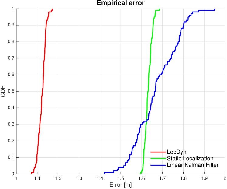
Figure 6: Empirical CDF for the planar lap trajectory with 100 Monte Carlo runs. LocDyn is the most accurate, and has a small variance in the empirical error. The Kalman filter fares the worst, mostly because of its slowdown behavior, as depicted in Figure 5.

But what about statistically relevant behavior? To answer this, we simulated the lap for 100 Monte Carlo trials and computed the empirical error of the trajectories. Figure 6 displays the resulting empirical cumulative distributions (CDF) for the three algorithms. Not only is LocDyn more accurate, but it also shows less variance in the error. The Kalman filter lags behind static localization, although it delivers smoother trajectories. This increase in the error is due to the bad accuracy near the slowdown points discussed previously.

V-B Descending spiral trajectory

Descending spirals are useful for monitoring the water column. They are difficult trajectories to follow so, although they are not associated with geophysical surveying activities, we tested LocDyn in them.

Figure 7: Example run: an AUV follows a descending spiral trajectory. Two algorithms attempt to localize it from noisy ranges and a few anchor positions. As expected, LocDyn has a natural trajectory and static localization scatters its estimates around the true trajectory.

Figure 7 shows an example run of the descending spiral trajectory. LocDyn has the smoothest trajectory, although both LocDyn and static localization are more deviated towards the center of the spiral. This is due to the small number of anchors in this setup, considering the augmented degrees of freedom in passing from 2D to 3D. Nevertheless, including dynamic information improves drastically the localization accuracy.

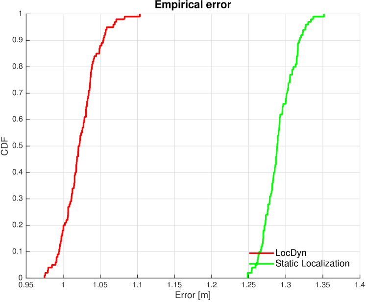
Figure 8: Empirical CDF for the descending spiral trajectory with 100 Monte Carlo runs. LocDyn is the most accurate estimator.

We documented the experimental accuracy increase in Figure 8. Here, we see the CDF of the empirical error from 100 Monte Carlo simulations. Noticeably, LocDyn confirms the intuition from the example trajectory of Figure 7: the average accuracy gain of using LocDyn is of 30cm — about one third of the 1m of measurement noise standard deviation.

V-C Lawn mower trajectory

In this experiment we test the robustness of the algorithms to outlier noise. Outliers are due, for example, to reflection or multi-path of the acoustic wave. At each step $k$ with probability $1\%$ the noisy range measurement of the vehicle to the anchor on the SW corner is doubled.

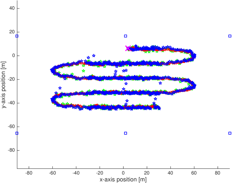
Figure 9: Example run: an AUV follows a lawn mower trajectory.

Figure 9 depicts one example run of the algorithms. At the outlier-contaminated steps we see that the Kalman filter looses the lawn mower path. Less frequently, static localization also increases the localization error.

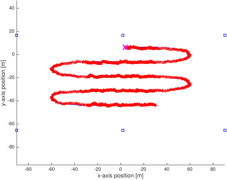
Figure 10: Example run: an AUV follows a lawn mower trajectory. LocDyn estimates.

Figure 10 displays only LocDyn estimates, and evidences that the trajectory was not particularly hurt.

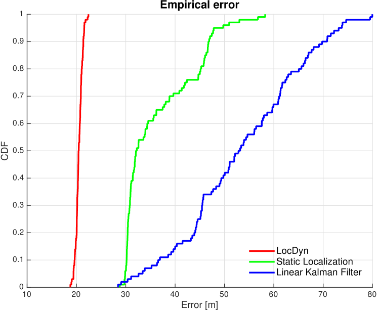
Figure 11: Empirical CDF for the lawn mower trajectory with 100 Monte Carlo runs. LocDyn is the most accurate estimator.

The empirical CDF demonstrates the impact of outlier noise in the positioning error, and confirms that LocDyn is not only the most accurate by far, but also with much less variance of the error.

VI Conclusion

We explored self-localization of a network of underwater vehicles from no more than noisy range measurements in a principled MAP estimation framework. We produced a fast, and distributed algorithm, LocDyn, topping in accuracy a comparable Kalman filter estimator. We showed the advantage of encoding the dynamic behavior of moving vehicles, by comparing LocDyn with a static network localization estimator. Also, we gave physical meaning to LocDyn’s only parameter, as a ratio of variability in measurement noise to variability of trajectories. An important open end of this work is to devise a way to eliminate the parameter altogether so to have a parameter-free solution for motion-aware network localization.

Appendix A $L$-smoothness and $m$-strong convexity of $g_{\lambda}$

$L$-smoothness implies that the gradient of $g_{\lambda}$ is Lipschitz continuous with Lipschitz constant $L$. A function $g$ is Lipschitz continuous if there exists a Lipschitz constant $L$ such that

$$\|g(x)-g(y)\|\leq L\|x-y\|,$$

for all $x$ and $y$. We now prove that the gradient of $g_{\lambda}$ is Lipschitz continuous and a Lipschitz constant $L$ can be identified by

$$\|\nabla g_{\lambda}(x)-\nabla g_{\lambda}(y)\| = \|\nabla\hat{f}(x)-\nabla\hat{f}(y)+2\lambda(x-y)\|$$ (13)

$$\leq \|\nabla\hat{f}(x)-\nabla\hat{f}(y)\|+2\lambda\|x-y\|$$

$$\leq \underbrace{(L_{\hat{f}}+2\lambda)}_{L}\|x-y\|.$$

The inequality (13) refers to the constant $L_{\hat{f}}$ in (16) of Soares et al. [16]. A strong convexity modulus $m$ for $g_{\lambda}$can be computed from

$$g_{\lambda}(x)-\frac{m}{2}x^{\top}x=\hat{f}(x)+\left(\lambda-\frac{m}{2}\right)x^{\top}x-2\lambda\tilde{x}^{\top}x+\lambda\tilde{x}^{\top}\tilde{x}$$

noticing that the left-hand side is convex if all terms in the right-hand side are convex in $x$. This entails that $g_{\lambda}$ is strongly convex with modulus

$$m\leq 2\lambda.$$

As we want robustness of $g_{\lambda}$ to errors in $x$, we choose $m$ to have the smallest condition number $L/m$ for function $g_{\lambda}$; thus, from now on we take the largest possible

$$m=2\lambda.$$ (14)

References

- [1] N. R. Council, Interim Report on 21st Century Cyber-Physical Systems Education. Washington, DC: The National Academies Press, 2015. [Online]. Available: https://www.nap.edu/catalog/21762/interim-report-on-21st-century-cyber-physical-systems-education
- [2] J. Kalwa, M. Carreiro-Silva, F. Tempera, J. Fontes, R. S. Santos, M. Fabri, L. Brignone, P. Ridao, A. Birk, T. Glotzbach et al., “The morph concept and its application in marine research,” in OCEANS-Bergen, 2013 MTS/IEEE. IEEE, 2013, pp. 1–8.
- [3] H. Al-Khatib, G. Antonelli, A. Caffaz, A. Caiti, G. Casalino, I. B. de Jong, H. Duarte, G. Indiveri, S. Jesus, K. Kebkal et al., “The widely scalable mobile underwater sonar technology (WiMUST) project: an overview,” in OCEANS 2015-Genova. IEEE, 2015, pp. 1–5.
- [4] P. C. Abreu, M. Bayat, J. Botelho, P. Góis, J. Gomes, A. Pascoal, J. Ribeiro, M. Ribeiro, M. Rufino, L. Sebastião, and H. Silva, “Cooperative formation control in the scope of the ec morph project: Theory and experiments,” in OCEANS 2015 - Genova, May 2015, pp. 1–7.
- [5] B. C. Pinheiro, U. F. Moreno, J. T. B. de Sousa, and O. C. Rodríguez, “Kernel-function-based models for acoustic localization of underwater vehicles,” IEEE Journal of Oceanic Engineering, vol. PP, no. 99, pp. 1–16, 2016.
- [6] H. J. Rad, T. Van Waterschoot, and G. Leus, “Cooperative localization using efficient kalman filtering for mobile wireless sensor networks,” in Signal Processing Conference, 2011 19th European. IEEE, 2011, pp. 1984–1988.
- [7] Y. Keller and Y. Gur, “A diffusion approach to network localization,” Signal Processing, IEEE Transactions on, vol. 59, no. 6, pp. 2642 –2654, June 2011.
- [8] Y. Shang, W. Rumi, Y. Zhang, and M. Fromherz, “Localization from connectivity in sensor networks,” Parallel and Distributed Systems, IEEE Transactions on, vol. 15, no. 11, pp. 961 – 974, Nov. 2004.
- [9] P. Biswas, T.-C. Liang, K.-C. Toh, Y. Ye, and T.-C. Wang, “Semidefinite programming approaches for sensor network localization with noisy distance measurements,” Automation Science and Engineering, IEEE Transactions on, vol. 3, no. 4, pp. 360 –371, Oct. 2006.
- [10] P. Oğuz-Ekim, J. Gomes, J. Xavier, and P. Oliveira, “Robust localization of nodes and time-recursive tracking in sensor networks using noisy range measurements,” Signal Processing, IEEE Transactions on, vol. 59, no. 8, pp. 3930 –3942, Aug. 2011.
- [11] Q. Shi, C. He, H. Chen, and L. Jiang, “Distributed wireless sensor network localization via sequential greedy optimization algorithm,” Signal Processing, IEEE Transactions on, vol. 58, no. 6, pp. 3328 –3340, June 2010.
- [12] S. Srirangarajan, A. Tewfik, and Z.-Q. Luo, “Distributed sensor network localization using SOCP relaxation,” Wireless Communications, IEEE Transactions on, vol. 7, no. 12, pp. 4886 –4895, Dec. 2008.
- [13] F. Chan and H. So, “Accurate distributed range-based positioning algorithm for wireless sensor networks,” Signal Processing, IEEE Transactions on, vol. 57, no. 10, pp. 4100 –4105, Oct. 2009.
- [14] U. Khan, S. Kar, and J. Moura, “DILAND: An algorithm for distributed sensor localization with noisy distance measurements,” Signal Processing, IEEE Transactions on, vol. 58, no. 3, pp. 1940 –1947, Mar. 2010.
- [15] A. Simonetto and G. Leus, “Distributed maximum likelihood sensor network localization,” Signal Processing, IEEE Transactions on, vol. 62, no. 6, pp. 1424–1437, Mar. 2014.
- [16] C. Soares, J. Xavier, and J. Gomes, “Simple and fast convex relaxation method for cooperative localization in sensor networks using range measurements,” Signal Processing, IEEE Transactions on, vol. 63, no. 17, pp. 4532–4543, Sept 2015.
- [17] G. Calafiore, L. Carlone, and M. Wei, “Distributed optimization techniques for range localization in networked systems,” in Decision and Control (CDC), 2010 49th IEEE Conference on, Dec. 2010, pp. 2221–2226.
- [18] C. Soares, J. Xavier, and J. Gomes, “Distributed, simple and stable network localization,” in Signal and Information Processing (GlobalSIP), 2014 IEEE Global Conference on, Dec 2014, pp. 764–768.
- [19] S. Schlupkothen, G. Dartmann, and G. Ascheid, “A novel low-complexity numerical localization method for dynamic wireless sensor networks,” IEEE Transactions on Signal Processing, vol. 63, no. 15, pp. 4102–4114, Aug 2015.
- [20] V. Ludovico, J. Gomes, J. Alves, and T. C. Furfaro, “Joint localization of underwater vehicle formations based on range difference measurements,” in 2014 Underwater Communications and Networking (UComms), Sept 2014, pp. 1–5.
- [21] B. Q. Ferreira, J. Gomes, C. Soares, and J. P. Costeira, “Collaborative localization of vehicle formations based on ranges and bearings,” in 2016 IEEE Third Underwater Communications and Networking Conference (UComms), Aug 2016, pp. 1–5.
- [22] B. Q. Ferreira, J. Gomes, and J. P. Costeira, “A unified approach for hybrid source localization based on ranges and video,” in 2015 IEEE International Conference on Acoustics, Speech and Signal Processing (ICASSP), April 2015, pp. 2879–2883.
- [23] J. Aspnes, T. Eren, D. K. Goldenberg, A. S. Morse, W. Whiteley, Y. R. Yang, B. D. Anderson, and P. N. Belhumeur, “A theory of network localization,” IEEE Transactions on Mobile Computing, vol. 5, no. 12, pp. 1663–1678, 2006.
- [24] S. Boyd and L. Vandenberghe, Convex Optimization. Cambridge University Press, Mar. 2004.
- [25] Y. Nesterov, Introductory Lectures on Convex Optimization: A Basic Course. Kluwer Academic Publishers, 2004.
- [26] L. Vandenberghe, “Fast proximal gradient methods,” EE236C course notes, Online, http://www.seas.ucla.edu/ vandenbe/236C/lectures/fgrad.pdf, 2014.
- [27] P. Holoborodko, “Smooth noise robust differentiators,” http://www.holoborodko.com/pavel/numerical-methods/numerical-derivative/smooth-low-noise-differentiators/, 2008.
- [28] S. Z. Khong, D. Nešić, Y. Tan, and C. Manzie, “Unified frameworks for sampled-data extremum seeking control: global optimisation and multi-unit systems,” Automatica, vol. 49, no. 9, pp. 2720–2733, 2013.
- [29] M. S. Hosseini and K. N. Plataniotis, “High-accuracy total variation with application to compressed video sensing,” IEEE Transactions on Image Processing, vol. 23, no. 9, pp. 3869–3884, 2014.
- [30] Y. Nesterov, “A method of solving a convex programming problem with convergence rate ,” in Soviet Mathematics Doklady, vol. 27, no. 2, 1983, pp. 372–376.