Interaction effects in a chaotic graphene quantum billiard

Abstract

We investigate the local electronic structure of a Sinai-like, quadrilateral graphene quantum billiard with zigzag and armchair edges using scanning tunneling microscopy at room temperature. It is revealed that besides the $(\sqrt{3}\times\sqrt{3})R30\degree$ superstructure, which is caused by the intervalley scattering, its overtones also appear in the STM measurements, which are attributed to the Umklapp processes. We point out that these results can be well understood by taking into account the Coulomb interaction in the quantum billiard, accounting for both the measured density of state values and the experimentally observed topography patterns. The analysis of the level-spacing distribution substantiates the experimental findings as well. We also reveal the magnetic properties of our system which should be relevant in future graphene based electronic and spintronic applications.

I Introduction

Quantum dots and quantum billiards have been in the focus of mesoscopic systems for the last three decades. The investigation of irregular shaped quantum billiards revealed how the classicaly chaotic behavior manifests in their energy spectrums.Bohigas et al. (1984); Berry (1985); Weidenmüller and Mitchell (2009); Mehta (2004) Although many properties of quantum dots with two-dimensional electron gas are now well understood, the appearance of new two-dimensional materials has renewed the interest in such systems both experimentally and theoretically. A paradigmatic example is graphene, the two-dimensional honeycomb lattice of carbon atoms, which has been an actively researched area since its discovery in 2004.Novoselov et al. (2004) Recent developments of nanofabrication and growth techniques make it now possible to create nanostructures with well-defined crystallographic edges.Tapasztó et al. (2008) Since they serve as building blocks of future nanodevices, it is crucial to understand their properties. As the Hamiltonian is different and various edge configurations can be present, it is not trivial how these effects alter the properties of quantum dots. An illustrative example is a classicaly chaotic neutrino billiard, investigated by Berry and Mondragon,Berry and Mondragon (1987) where the energy spectrum turned out to be governed by the Gaussian Unitary Ensemble (GUE) instead of the Gaussian Orthogonal Ensemble (GOE) as one would naively expect, since time-reversal symmetry seems to be present at first glance. The Hamiltonian of graphene is similar to that of the neutrino billiards, however, the various edge types can lead to further effects.Wurm et al. (2009, 2011) This is the reason why special attention has been paid to graphene based billiards.Wurm et al. (2009, 2011); Huang et al. (2011); Hämäläinen et al. (2011); Ponomarenko et al. (2008); Rycerz (2012, 2013); Ying et al. (2014); Jolie et al. (2014); Ramos et al. (2014, 2016) It has been shown that in the absence of intervalley scattering, which case is identical to the neutrino billiard, the level-spacing distribution follows GUE statistics.Wurm et al. (2009, 2011) However, when the valleys are not independent the time-reversal symmetry is restored, the level-spacing distribution obeys GOE statistics. Wurm et al. (2009, 2011)

Although many properties of bulk graphene can be understood within a noninteracting picture, interaction effects can become important if one considers finite samples. Even a weak electron-electon interaction can lead to drastic effects, for example, in zigzag graphene nanoribbons the paramagnetic ground state becomes unstable against magnetic ordering.Son et al. (2006); Yang et al. (2007); Wassmann et al. (2008); Fernández-Rossier (2008); Yazyev (2008); Jung and MacDonald (2009); Feldner et al. (2011); Golor et al. (2014); Hagymási and Legeza (2016) This is due to the fact that the zigzag edge states form a flat band at the Fermi energy and the corresponding large density of states is not favorable energetically in the presence of the interaction, therefore a symmetry-breaking ground state occurs. The same scenario can happen in graphene quantum dots possessing zigzag edges.Ezawa (2007); Feldner et al. (2010)

In this paper we examine a quadrilateral shaped graphene quantum dot, which is a truncated triangle having three zigzag and one armchair edges. This peculiar shape resembles the theoretically well-studied Sinai billiard.Stöckmann (1999) In this joint experimental and theoretical study, we use scanning tunneling microscopy (STM) and perform theoretical calculations to understand the experimental results. Our main finding is that the electron-electron interaction must be taken into account to reproduce the STM images and local density of states (LDOS) measurements which highlight the important role of the interactions in graphene quantum dots even at room temperature. The results may have implications in the nanoscale engineering of the electronic and magnetic properties of graphene based functional surfaces.

The paper is organized as follows. In Sec. II. A the investigated quantum dot is introduced together with the experimental details, while in Sec. II. B the applied theoretical methods are described. In Sec. III. A we examine the properties of the noninteracting quantum billiard using the elements of quantum chaos. In Sec. III. B we discuss the experimental results together with our theoretical findings. Sec. III. C presents the magnetic properties of the quantum dot based on the theoretical results. Finally, in Sec. IV.  our conclusions are presented.

II Methods

II.1 Experimental details

Graphene grown by chemical vapour deposition onto electro-polished copper foilPálinkás et al. (2016) was transferred onto highly oriented pyrolytic graphite (HOPG) substrate using thermal release tape. An etchant mixture consisting of CuCl2 aqueous solution (20%) and hydrochloric acid (37%) in 4:1 volume ratio was used. After etching the copper foil, the tape holding the graphene was rinsed in distilled water, then dried and pressed onto the HOPG surface. The tape/graphene/HOPG sample stack was placed onto a hot plate at 95 $\degree$C. At this temperature the tape released the graphene and it could be removed easily. Graphene nanostructures were obtained by annealing the graphene/HOPG sample at 650 $\degree$C for two hours in argon atmosphere. STM and tunneling spectroscopy (STS) measurements were performed using a DI Nanoscope E operating under ambient conditions. The investigated graphene quantum dot is a truncated triangle, as shown in Fig. 1 (a). Atomic resolution images obtained on the dot (inset of Fig. 1 (a)) reveal that the nanostructure has three zigzag edges and one armchair edge. The formation of predominantly zigzag edges is due to the fact that these edges are more resistive to thermal oxidation.Nemes-Incze et al. (2010)

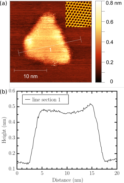
Figure 1: (a) STM image of the investigated graphene quantum dot. Tunneling parameters: $U=200$ mV, $I=1$ nA. The atomic resolution inset image shows the crystallographic orientation in the dot. (b) Height profile taken along the line section 1 in (a), showing monolayer thickness.

II.2 Theory

To describe the graphene quantum dot, we use the $\pi$-band model of graphene, where a lattice site can host two electrons at most with opposite spins. We consider nearest-neighbor hopping terms only, and model the Coulomb repulsion by using a local Hubbard interaction term. Thus, we arrive at the Hamiltonian:

$$\mathcal{H}=-t\sum_{\langle ij\rangle\sigma}\hat{c}^{\dagger}_{i\sigma}\hat{c}^{\phantom{\dagger}}_{j\sigma}+U\sum_{i}\hat{n}_{i\uparrow}\hat{n}_{i\downarrow}-\mu\sum_{i\sigma}\hat{n}_{i\sigma},$$ (1)

where the summation $\langle ij\rangle$ extends over all nearest-neighbor pairs. The operator $\hat{c}^{\dagger}_{i\sigma}$ ($\hat{c}^{\phantom{\dagger}}_{i\sigma}$) creates (annihilates) an electron at site $i$ with spin $\sigma$ and $\hat{n}_{i\sigma}$ is the corresponding particle number operator. The nearest-neighbor hopping amplitude is given by $t$, $U$ is the onsite Hubbard interaction strength and $\mu$ is the chemical potential. Throughout the paper we set $t=3\ {\rm eV}$, which defines the energy scale of the system and tune the chemical potential close to the half-filled case to account for the small $p$-doping in the experiment. We assume a weak Coulomb repulsion $U/t=1$, in agreement with previous experiments.Magda et al. (2014) Since the Hamiltonian (1) can be solved exactly for very small systems, we must use approximations to obtain results for realistic systems. The most commonly used one is the mean-field approach, whose application is justified for moderate values of electron-electron interaction in case of graphene nanodisks.Feldner et al. (2010) By neglecting the fluctuation terms in the Hamiltonian (1), we obtain an effective single-particle Hamiltonian

$$\mathcal{H}_{\rm MF}=-t\sum_{\langle ij\rangle\sigma}\hat{c}^{\dagger}_{i\sigma}\hat{c}^{\phantom{\dagger}}_{j\sigma}+U\sum_{i\sigma}\langle\hat{n}_{i\bar{\sigma}}\rangle\hat{n}_{i\sigma}-\mu\sum_{i\sigma}\hat{n}_{i\sigma},$$ (2)

where the unknown electron densities, $\langle\hat{n}_{i\bar{\sigma}}\rangle$ are determined by using the standard self-consistent procedure and $\mu$ is determined by the conservation of the electron number. Having obtained the mean-field solution one can calculate then the LDOS in the quantum dot as a function of energy from the Green function:

$$\rho_{i}(E)=-\frac{1}{\pi}{\rm Im}\ G_{ii}(E)=-\frac{1}{\pi}{\rm Im}((E+i0^{+})I-\mathcal{H}_{\rm MF})^{-1}_{ii},$$ (3)

where $I$ is the identity operator.

III Results

III.1 Noninteracting case

Before diving into the details of the experimental and theoretical results, it is worth investigating what we can learn from the noninteracting tight-binding picture. Therefore, we perform tight-binding calculations for this peculiar geometry, a truncated triangle with zigzag and armchair edges, shown in Fig. 1 (a). To account for the edge roughness and to obtain a more realistic geometry, we removed randomly certain edge atoms as shown in Fig. 2.

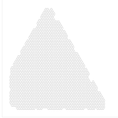
Figure 2: The geometry used in the model calculations. The dot consists of 4310 atoms.

Thus our model contains 4310 atoms. We calculate the energy spectrum by diagonalizing the tight-binding Hamiltonian, which is shown in Fig. 3 ($U/t=0$).

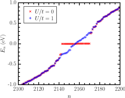
Figure 3: The energy spectrum of the quantum dot near the Fermi-energy with and without the Hubbard term. The role of the interaction is discussed in Sec. II. B.

It is observed that the zero-energy states, which correspond to the Fermi level, are multiply degenerate. This may not surprise us if we recall that zigzag-shaped nanodisks also have degenerate zero-energy states, which are attributed to the presence of edge-localized states.Ezawa (2007) It is worth mentioning that this degeneracy is still present but partially resolved in our case due to the armchair edge and edge defects.

To reveal the properties of integrability, we examine the level-spacing distribution, $P(S)$. This quantity reflects the nature of the corresponding classical dynamics of the system and follows certain university classes depending on the Hamiltonian.Weidenmüller and Mitchell (2009); Mehta (2004) By definition, $P(S)dS$ gives the probability that the distance between the neighboring values of the unfolded spectrum, $\langle\rho(E)\rangle(E_{i+1}-E_{i})$, lies in the interval $(S,S+dS)$, where $E_{i}$ are the eigenvalues of the tight-binding Hamiltonian and $\langle\rho(E)\rangle$ is the average density of states in the interval $(E,E+dE)$. In graphene quantum billiards, we can approximate this quantity by its bulk value:

$$\langle\rho(E)\rangle\approx\rho_{\rm bulk}(E)=\frac{1}{\pi}\frac{\cal A}{(\hbar v_{F})^{2}}|E|,$$ (4)

where $\mathcal{A}$ is the area of the quantum billiard, $v_{F}$ is the Fermi velocity. According to our previous definition in Sec. II. B, $t=\frac{2}{3}\sqrt{3}\hbar v_{F}/a\approx 3\ {\rm eV}$ and $a$ is the lattice spacing of graphene. In completely integrable systems, the energy levels are uncorrelated, and their level-spacing statistics follows Poisson distribution:

$$P(S)=\exp(-S).$$ (5)

In chaotic systems with (or without) time-reversal symmetry the level-spacing obeys the GOE (or GUE) of random matrices:Weidenmüller and Mitchell (2009); Mehta (2004)

$$P_{\rm GOE}(S) =\frac{\pi}{2}S\exp\left(-\frac{\pi S^{2}}{4}\right),$$ (6)

$$P_{\rm GUE}(S) =\frac{32}{\pi^{2}}S^{2}\exp\left(-\frac{4S^{2}}{\pi}\right).$$ (7)

It is worth noting that in integrable systems energy levels lie close to each other, since the probability distribution is maximal at $S=0$. In contrast, chaotic systems exhibit level repulsion since the corresponding probability densities vanish as $S\to 0$, which is often referred as avoided level crossings. The zero-energy states, which are essentially degenerate, are due to the zigzag edges and localized on segments of the zigzag boundaries. Since they would cause an artificial contribution in the level distribution, we consider the interval $0.1\lesssim E/t\lesssim 1$, which contains approximately 400 eigenvalues. The level spacing distribution for our noninteracting quadrilateral graphene billiard is shown in Fig. 4 together with the distribution functions Eqs. (5)-(7) corresponding to the university classes.

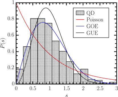
Figure 4: The level-spacing distribution obtained from the unfolded spectrum. The solid red, blue and black lines correspond to the Poisson, GOE and GUE distributions.

In contrast to the equilateral triangle billiard which is an integrable systemRycerz (2012) our results clearly indicate that our quantum billiard is a classicaly chaotic system. Moreover, the calculated level-spacings are in a very good agreement with the GOE statistics and not with the GUE as one might expect based on the connection with the neutrino billiard. This confirms what has been mentioned in Sec. I that the two valleys are coupled to each other due to the armchair edge and the defects on the zigzag edges, which restore the time-reversal symmetry of the quantum billiard.

III.2 Experimental results and their theoretical explanations

In the previous subsection we have demonstrated that our quantum dot is a chaotic billiard based on its level-spacing distribution and the corresponding university class is GOE, which suggests strong intervalley scattering. In what follows we show direct experimental evidence which supports this scenario and also demonstrate how the electron-electron interaction modifies the measured properties of the system.

First of all, we discuss the measured ${\rm d}I/{\rm d}V$ spectra which correspond to the LDOS of the systems. The experimental results measured in the middle of the quantum dot and on the HOPG substrate are shown in Fig. 5.

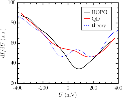
Figure 5: The measured LDOS as a function of the voltage, the solid black and red lines correspond to the HOPG substrate and the quantum dot, respectively. The dotted blue line represents the theoretical result for the LDOS of the quantum dot. In the theoretical calculation a Gaussian broadening $0.1$ eV is used to account for the finite temperature.

The measured HOPG LDOS exhibits the known linear behavior, but it is asymmetric with respect to the Dirac point and has a finite amount of $p$-doping (80 meV) due to impurities in the system.

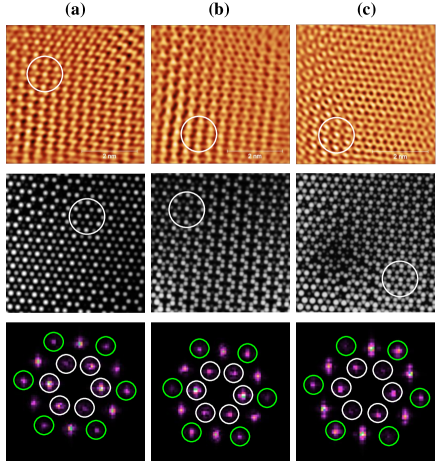
Figure 6: The topographic STM images within the quantum dot. Each column corresponds to different voltages where the measurement was done: (a), (b) and (c) belong to $U=100$ mV, 25 mV and -50 mV, respectively. The first row shows the measured images, the second one contains the simulated images, while the third row displays the Fourier spectrum of the measured images. The spots inside the white circles in the Fourier spectrum are the components of the $(\sqrt{3}\times\sqrt{3})R30\degree$ superstructure, while the green circled spots are their overtones. The non-circled spots correspond to the periodicity of the atomic lattice.

It is easily seen that the quantum dot exhibits similar behavior to the HOPG far from the Fermi energy, however, higher LDOS appears near the Dirac point. If we recall the energy spectrum of the noninteracting system in Fig. 3, we observe that a gap $\Delta\sim 0.2$ eV is opened, which is not visible in the measured LDOS. (We also investigated the role of the next-nearest-neighbor (NNN) hopping term on the spectrum of the quantum dot, since it may result in similar effectsWimmer et al. (2010). We found that the inclusion of NNN hopping lifts the degeneracy at the Fermi level, but the observed band gap quantitatively remains unchanged. See Appendix for details.) This is the first indication that the noninteracting model does not describe the dot accurately. We know that such highly degenerate levels near the Fermi-energy are very sensitive to even weak electron-electron interaction, just like in graphene nanoribbons with zigzag edges. Switching on the interaction, we can see from Fig. 3 that the energy levels near the Fermi-energy are no longer degenerate even for a small value of the Hubbard-$U$, $U/t=1$, while the high-lying states are not modified. (Note that this weak interaction does not alter the energy levels, where the level-spacing distribution was taken.) Thus, the obtained spectrum with electron-electron interaction is much closer to what we expect from the LDOS measurements in Fig. 5. In order to compare the results we also plot the calculated LDOS inside the quantum dot taking into account the finite $p$-doping (Fig. 5). The measured and the calculated values are in good agreement, however, some discrepancy is observed slightly below the Fermi energy, where the calculated minimum does not appear. This can be understood considering that the LDOS of HOPG is asymmetric, therefore its slope below the Fermi energy is larger than above it. Since the HOPG also contributes to the tunneling current, their larger LDOS values can vanish the calculated LDOS minimum of the dot below the Fermi energy.

In the following we discuss the measured topographic STM images. In Fig. 6 we can see superstructure patterns within the quantum dot measured at various voltages. Regarding the voltages, $U=100$, 25 and -50 mV, where the STM images were taken, and the energy spectrum in Fig. 3, then it is evident that the noninteracting tight-binding description fails. Since these energy values lie in the gap there is no way to account for the different STM images. In contrast, Fig 6 shows clearly different superstructure patterns. In Fig. 6 (a) the well-known $(\sqrt{3}\times\sqrt{3})R30\degree$ superstructure (marked by white circle) appears on the top of the atomic structure. This is more spectacular from the Fourier spectrum in Fig. 6 (a), where the components of the superstructure are clearly seen (marked by white circles). Since this structure originates from the intervalley scattering between the $K$ and $K^{\prime}$ valleys due to the presence of the armchair edge,Niimi et al. (2006); Sakai et al. (2010) it confirms our previous theoretical findings based on the level-spacing distribution (Fig. 4) where the intervalley scattering was predicted by the GOE distribution. In Fig. 6 (b)-(c) besides the $(\sqrt{3}\times\sqrt{3})R30\degree$ superstructure, stripes parallel to armchair edge and rings are observed in the measured STM images. In order to simulate these distinct STM images, we consider a finite electron-electron interaction using the procedure described in Sec. II. B. With the help of the calculated LDOS of the interacting system, we simulate the STM images with the simple Tersoff-Hamann approximation.Tersoff and Hamann (1985) Taking into account the electron-electron interaction, we can quantitatively reproduce the measured STM images, including the $(\sqrt{3}\times\sqrt{3})R30\degree$ superstructure in Fig. 6 (a), the stripes in Fig. 6 (b), and the rings in Fig. 6 (c) at the different voltages. If we take a closer look to the measured Fourier spectra, it can be easily seen that the Fourier components of the $(\sqrt{3}\times\sqrt{3})R30\degree$ superstructure are always present (inner hexagon, components marked with white circles). Moreover, their overtones (marked with green circles) appear with various amplitudes which results in the formation of different, more complex patterns in the topography images. The emergence of the overtones measured by STM can be attributed to the Umklapp scattering processes, where an electron is scattered outside the first Brillouin Zone (BZ). Thus, in our quantum dot besides the usual scattering between $K$ and $K^{\prime}$ valleys in first BZ ($\boldsymbol{K-K^{\prime}=q}$), electrons also scatter from the first BZ $K$ valley to the second BZ $K^{\prime}$ valley ($\boldsymbol{K-K^{\prime}=q+G}$). This latter is equal to the shift of the $K^{\prime}$ point back to the first BZ by a reciprocal lattice vector $\boldsymbol{G}$. Beacuse the Umklapp processes are absent in the noninteracting case and they appear if electron-electron interaction is present in the half-filled Hubbard model,Ehlers et al. (2015) it serves as a further evidence for the presence of electron-electron interaction in our system.

III.3 Magnetic properties

Previously, we demonstrated that the inclusion of the electron-electron interaction provides a good agreement with the experimental results in terms of the measured LDOS and topographic STM images. Since our quantum dot is a quite complex system including doping and edge defects, it is worth revealing the effects of the interaction expicitly by considering the magnetic moments at the lattice sites. It has been mentioned earlier that the paramagnetic state becomes unstable against magnetic ordering if zigzag edges are present in the system,Feldner et al. (2010); Hagymási and Legeza (2016); Valli et al. (2016) however, it also known that the presence of doping can vanish the appeared magnetic moments.Potasz et al. (2012) To clarify the presence of the magnetism in our system we calculated the magnetic moments by taking into account the measured $p$-doping (80 meV). We found that magnetic moments are still present in the doped system (Fig. 7 (b)), although their values are smaller than in the half-filled case (Fig. 7 (a)).

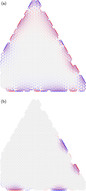
Figure 7: Magnetic moments in the quantum dot for $U/t=1$. Panels (a) and (b) correspond to the half-filled case and 80 meV $p$-doping, respectively. The blue and red colors encode the up and down spins, respectively. The magnitude of the spins depends on the radii of the circles, $r$, as $\exp(-r)$. The largest magnetic moments in both cases are $S_{z}\sim 0.12$.

Quantitatively, the average momentum of up- and down-spin electrons in the doped quantum dot is decreased to one fourth of the undoped value. This reduction can be seen also in Fig. 7 (b), where the magnetic moments disappeared along the shortest zigzag side of the triangle and are localized only at the longer zigzag edge segments. We note that for larger doping values (120 meV) the magnetic moments totally vanish at the edges, which is consistent with previous findings.Potasz et al. (2012) Our calculations indicate that only the zigzag edges are magnetic and no magnetization occurs along the armchair edge and around the defects in the zigzag edges. It is in agreement with the a priori expectations based on nanoribbons, since armchair nanoribbons are not magnetic, and edge defects in zigzag ribbons suppress the magnetism.Magda et al. (2014); Wu et al. (2010) This follows from the fact that here the sublattice symmetry is restored, while zigzag edges contain atoms only from one sublattice. We also observe spin-collinear domain wallsYazyev and Katsnelson (2008) along the edges due to presence of the defects. Overall, we can conclude that the magnetism can be present in the system even at the presence of small doping and edge defects based on the mean-field calculations. Our analysis above gives further insight into the role of the electron-electron interaction in graphene quantum dots.

IV Conclusions

We carried out a joint experimental and theoretical investigation to analyze the properties of a quadrilateral shaped graphene quantum billiard. First, we examined the quantum billiard in a tight-binding picture to grasp the properties of integrability. It turned out that the billiard is chaotic, moreover, its level-spacing distribution agree well with the GOE distribution. This indicates strong intervalley scattering, which also manifests in the appearance of the $(\sqrt{3}\times\sqrt{3})R30\degree$ superstructure observed in the STM images measured under ambient conditions. We pointed out that by taking into account the interaction among the electrons, we were able to elucidate the spectroscopy (LDOS) measurements and STM images simultaneously. Using the mean-field approximation of the Hubbard model we reproduced the $(\sqrt{3}\times\sqrt{3})R30\degree$, stripe and ring superstructures as well. It was also revealed that the latter two structures appear due to the overtones of the Fourier components of $(\sqrt{3}\times\sqrt{3})R30\degree$ superstructure, which also confirms the importance of the interaction even at room-temperature. Furthermore, we showed that the weak electron-electron interaction does not alter the higher energy levels ($>0.2$ eV), only the ones near the Dirac point (lifted degeneracy). Thus the chaotic nature and the time-reversal symmetry of the graphene billiard is preserved. We also demonstrated that edge-magnetism appears along the zigzag edges, and the magnetic moments disappear inside the quantum dot. The ability of tailoring the electronic and magnetic properties of graphene quantum dots can open new avenues for information coding at nanoscale.

Appendix A The role of next-nearest-neighbor hopping

In order to understand the lack of energy gap in the ${\rm d}I/{\rm d}V$ spectra and the role of the interaction it is important to consider other effects that may alter the energy spectrum. The most important candidate is the next-nearest-neighbor (NNN) hopping, since it is known to break the electron-hole symmetry and shifts the dispersionless edge states away from the zero energy.Wimmer et al. (2010) Therefore, we study the following Hamiltonian:

$$\mathcal{H}=-t\sum_{\langle ij\rangle\sigma}\hat{c}^{\dagger}_{i\sigma}\hat{c}^{\phantom{\dagger}}_{j\sigma}-t^{\prime}\sum_{\langle\langle ij\rangle\rangle\sigma}\hat{c}^{\dagger}_{i\sigma}\hat{c}^{\phantom{\dagger}}_{j\sigma}+U\sum_{i}\hat{n}_{i\uparrow}\hat{n}_{i\downarrow},$$ (8)

where $\langle\langle ij\rangle\rangle$ denotes the summation over all NNN pairs. For the value of $t^{\prime}$ we use $t^{\prime}=0.1$ eV from the tight-binding fit to experimental data.Deacon et al. (2007); Castro Neto et al. (2009) To reveal the effect of NNN hopping, we calculated the energy spectrum of the Hamiltonian (8) in the noninteracting case, which is shown in Fig. 8.

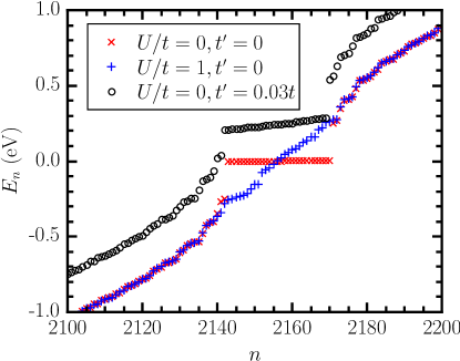
Figure 8: The energy spectrum of the quantum dot near the Fermi-energy with and without NNN hopping terms. For better comparison, the result for the interacting case is shown too.

It is obviously seen that the NNN hopping lifts the degeneracy of the edge states, and they are slightly shifted towards higher energies. However, they still lie very close to each other, and the gap $\Delta\sim 0.2$ eV in the spectrum hardly decreases. In contrast, the interaction completely removes the degeneracy of the zero-energy states and the gap disappears in the spectrum.

References

- Bohigas et al. (1984) O. Bohigas, M. J. Giannoni, and C. Schmit, Phys. Rev. Lett. 52, 1 (1984).
- Berry (1985) M. V. Berry, Proc. R. Soc. London Ser. A 400, 229 (1985).
- Weidenmüller and Mitchell (2009) H. A. Weidenmüller and G. E. Mitchell, Rev. Mod. Phys. 81, 539 (2009).
- Mehta (2004) M. L. Mehta, Random Matrices, 3rd ed. (Elsevier, Amsterdam, 2004).
- Novoselov et al. (2004) K. S. Novoselov, A. K. Geim, S. V. Morozov, D. Jiang, Y. Zhang, S. V. Dubonos, I. V. Grigorieva, and A. A. Firsov, Science 306, 666 (2004).
- Tapasztó et al. (2008) L. Tapasztó, G. Dobrik, P. Lambin, and L. P. Biró, Nat. Nano. 3, 397 (2008).
- Berry and Mondragon (1987) M. V. Berry and R. J. Mondragon, Proc. R. Soc. London Ser. A 412, 53 (1987).
- Wurm et al. (2009) J. Wurm, A. Rycerz, I. Adagideli, M. Wimmer, K. Richter, and H. U. Baranger, Phys. Rev. Lett. 102, 056806 (2009).
- Wurm et al. (2011) J. Wurm, K. Richter, and I. Adagideli, Phys. Rev. B 84, 205421 (2011).
- Huang et al. (2011) L. Huang, Y.-C. Lai, and C. Grebogi, Chaos 21, 013102 (2011).
- Hämäläinen et al. (2011) S. K. Hämäläinen, Z. Sun, M. P. Boneschanscher, A. Uppstu, M. Ijäs, A. Harju, D. Vanmaekelbergh, and P. Liljeroth, Phys. Rev. Lett. 107, 236803 (2011).
- Ponomarenko et al. (2008) L. A. Ponomarenko, F. Schedin, M. I. Katsnelson, R. Yang, E. W. Hill, K. S. Novoselov, and A. K. Geim, Science 320, 356 (2008).
- Rycerz (2012) A. Rycerz, Phys. Rev. B 85, 245424 (2012).
- Rycerz (2013) A. Rycerz, Phys. Rev. B 87, 195431 (2013).
- Ying et al. (2014) L. Ying, G. Wang, L. Huang, and Y.-C. Lai, Phys. Rev. B 90, 224301 (2014).
- Jolie et al. (2014) W. Jolie, F. Craes, M. Petrović, N. Atodiresei, V. Caciuc, S. Blügel, M. Kralj, T. Michely, and C. Busse, Phys. Rev. B 89, 155435 (2014).
- Ramos et al. (2014) J. G. G. S. Ramos, I. M. L. da Silva, and A. L. R. Barbosa, Phys. Rev. B 90, 245107 (2014).
- Ramos et al. (2016) J. G. G. S. Ramos, M. S. Hussein, and A. L. R. Barbosa, Phys. Rev. B 93, 125136 (2016).
- Son et al. (2006) Y.-W. Son, M. L. Cohen, and S. G. Louie, Phys. Rev. Lett. 97, 216803 (2006).
- Yang et al. (2007) L. Yang, C.-H. Park, Y.-W. Son, M. L. Cohen, and S. G. Louie, Phys. Rev. Lett. 99, 186801 (2007).
- Wassmann et al. (2008) T. Wassmann, A. P. Seitsonen, A. M. Saitta, M. Lazzeri, and F. Mauri, Phys. Rev. Lett. 101, 096402 (2008).
- Fernández-Rossier (2008) J. Fernández-Rossier, Phys. Rev. B 77, 075430 (2008).
- Yazyev (2008) O. V. Yazyev, Phys. Rev. Lett. 101, 037203 (2008).
- Jung and MacDonald (2009) J. Jung and A. H. MacDonald, Phys. Rev. B 79, 235433 (2009).
- Feldner et al. (2011) H. Feldner, Z. Y. Meng, T. C. Lang, F. F. Assaad, S. Wessel, and A. Honecker, Phys. Rev. Lett. 106, 226401 (2011).
- Golor et al. (2014) M. Golor, S. Wessel, and M. J. Schmidt, Phys. Rev. Lett. 112, 046601 (2014).
- Hagymási and Legeza (2016) I. Hagymási and Ö. Legeza, Phys. Rev. B 94, 165147 (2016).
- Ezawa (2007) M. Ezawa, Phys. Rev. B 76, 245415 (2007).
- Feldner et al. (2010) H. Feldner, Z. Y. Meng, A. Honecker, D. Cabra, S. Wessel, and F. F. Assaad, Phys. Rev. B 81, 115416 (2010).
- Stöckmann (1999) H.-J. Stöckmann, Quantum Chaos - An Introduction (University Press, Cambridge, 1999).
- Pálinkás et al. (2016) A. Pálinkás, P. Süle, M. Szendrő, G. Molnár, C. Hwang, L. P. Biró, and Z. Osváth, Carbon 107, 792 (2016).
- Nemes-Incze et al. (2010) P. Nemes-Incze, G. Magda, K. Kamarás, and L. P. Biró, Nano Res. 3, 110 (2010).
- Magda et al. (2014) G. Z. Magda, X. Jin, I. Hagymási, P. Vancsó, Z. Osváth, P. Nemes-Incze, C. Hwang, L. P. Biró, and L. Tapasztó, Nature 514, 608 (2014).
- Wimmer et al. (2010) M. Wimmer, A. R. Akhmerov, and F. Guinea, Phys. Rev. B 82, 045409 (2010).
- Niimi et al. (2006) Y. Niimi, T. Matsui, H. Kambara, K. Tagami, M. Tsukada, and H. Fukuyama, Phys. Rev. B 73, 085421 (2006).
- Sakai et al. (2010) K.-i. Sakai, K. Takai, K.-i. Fukui, T. Nakanishi, and T. Enoki, Phys. Rev. B 81, 235417 (2010).
- Tersoff and Hamann (1985) J. Tersoff and D. R. Hamann, Phys. Rev. B 31, 805 (1985).
- Ehlers et al. (2015) G. Ehlers, J. Sólyom, Ö. Legeza, and R. M. Noack, Phys. Rev. B 92, 235116 (2015).
- Valli et al. (2016) A. Valli, A. Amaricci, A. Toschi, T. Saha-Dasgupta, K. Held, and M. Capone, Phys. Rev. B 94, 245146 (2016).
- Potasz et al. (2012) P. Potasz, A. D. Güçlü, A. Wójs, and P. Hawrylak, Phys. Rev. B 85, 075431 (2012).
- Wu et al. (2010) W. Wu, Z. Zhang, P. Lu, and W. Guo, Phys. Rev. B 82, 085425 (2010).
- Yazyev and Katsnelson (2008) O. V. Yazyev and M. I. Katsnelson, Phys. Rev. Lett. 100, 047209 (2008).
- Deacon et al. (2007) R. S. Deacon, K.-C. Chuang, R. J. Nicholas, K. S. Novoselov, and A. K. Geim, Phys. Rev. B 76, 081406 (2007).
- Castro Neto et al. (2009) A. H. Castro Neto, F. Guinea, N. M. R. Peres, K. S. Novoselov, and A. K. Geim, Rev. Mod. Phys. 81, 109 (2009).