Bose- Einstein condensation of triplons with a weakly broken U(1) symmetry

Abstract

The low-temperature properties of certain quantum magnets can be described in terms of a Bose-Einstein condensation (BEC) of magnetic quasiparticles (triplons). Some mean-field approaches (MFA) to describe these systems, based on the standard grand canonical ensemble, do not take the anomalous density into account and leads to an internal inconsistency, as it has been shown by Hohenberg and Martin, and may therefore produce unphysical results. Moreover, an explicit breaking of the U(1) symmetry as observed, for example, in TlCuCl₃ makes the application of MFA more complicated. In the present work, we develop a self-consistent MFA approach, similar to the Hartree-Fock-Bogolyubov approximation in the notion of representative statistical ensembles, including the effect of a weakly broken U(1) symmetry. We apply our results on experimental data of the quantum magnet TlCuCl₃ and show that magnetization curves and the energy dispersion can be well described within this approximation assuming that the BEC scenario is still valid. We predict that the shift of the critical temperature $T_{c}$ due to a finite exchange anisotropy is rather substantial even when the anisotropy parameter $\gamma$ is small, e.g., $\Delta T_{c}\approx 10\%$ of $T_{c}$ in $H$= 6 T and for $\gamma\approx 4\rm{\mu eV}$.

Keywords:Quantum magnets, TlCuCl₃, BEC, triplons, explicitly broken gauge symmetry, anisotropy , critical temperature, magnetization curves, anomalous density

1 Introduction

Spontaneous symmetry breaking (SSB) plays an important role in particle and condensed matter physics. In the Standard Model of particle physics SSB of gauge symmetries is responsible for generating masses for several particles and separating the electromagnetic and weak forces [1]. In condensed matter physics SSB lies in the origin of effects such as Bose-Einstein condensation (BEC), superconductivity, ferromagnetism etc. In terms of microscopical field-theoretical models SSB corresponds to the case when the Hamiltonian of the system is invariant under a given transformation, while its ground state is not. Particularly, BEC is related to the U(1) symmetry of the Hamiltonian as $\psi(\mathbf{r})\rightarrow\psi(\mathbf{r})e^{i\alpha}$ for the field operator $\psi(\mathbf{r})$, with $\alpha$ being a real number. Moreover, strictly speaking, spontaneous symmetry breaking is a sufficient condition for the occurrence of BEC [2]. Remarkably, not only real particles, but also quasiparticles may undergo BEC. In 1999 Oosawa et al [3] performed magnetization measurements to investigate the critical behavior of the field-induced magnetic ordering in the quantum antiferromagnetic TlCuCl₃. Changing the external magnetic field in the range of $H_{\rm{ext}}\sim$ 5 T $\div$ 7 T they observed an unexpected inflection of the magnetization curve, i.e. $M(T,H)$, when $H_{\rm{ext}}$ exceeds a critical value, $H_{\rm{ext}}>$ $H_{c}$.

In fact, as it is seen from Fig.3 of Ref. [3] , for $H_{\rm{ext}}>$5.3 T there is a critical temperature $T_{c}$($H_{\rm{ext}}$) below which the magnetization of the antiferromagnet starts to increase. Later on due to the works by Rüegg [4], Yamada [5] and Nikuni [6], who obtained similar results as in [3], the following interpretation of this phenomenon has been established :

1. In some compounds such as KCuCl₃ or TlCuCl₃ two Cu²⁺⁺ ions are antiferromagnetially coupled to form a dimer in a crystalline network: the dimer ground state is a spin singlet (S=0), separated by an energy gap from the first excited triplet state with S=1.

2. At a critical external magnetic field, the energy of one of the Zeeman split triplet components intersects the ground state singlet and the gap between these two state may be closed.

3. The appropriate quasiparticles, in the following called triplons, undergo BEC below a critical temperature, $T\leq T_{c}$.

4. The whole density of triplons, $\rho$ and the density of condensed triplons, $\rho_{0}$, defines the $M_{\parallel}$ and $M_{\perp}$ magnetizations per Cu atom. Namely, $M_{\parallel}\sim\rho$ and $M_{\perp}\sim\sqrt{\rho_{0}}$.

5. The density of triplons is directly controlled by the applied magnetic field which acts as a chemical potential.

6. The thermodynamic characteristics as well as the magnetization may be calculated with a simple effective Hamiltonian

   $$H=\sum_{\mathbf{k}}(\varepsilon_{k}-\mu)a_{\mathbf{k}}^{{\dagger}}a_{\mathbf{k}}+\frac{U}{2}\sum_{\mathbf{k},\mathbf{k}^{\prime},\mathbf{q}}a_{\mathbf{k}+\mathbf{q}}^{{\dagger}}a_{\mathbf{k}^{\prime}-\mathbf{q}}^{{\dagger}}a_{\mathbf{k}}a_{\mathbf{k}^{\prime}}$$ (1)

   where $\varepsilon_{\mathbf{k}}$ is the kinetic energy determined by the dispersion around the lowest excitation, $\mu$ is the chemical potential given by

   $$\mu=g\mu_{B}(H_{\rm{ext}}-H_{c}),$$ (2)

   $U$ is the interaction constant, and $a_{\mathbf{k}}^{{\dagger}}(a_{\mathbf{k}})$ are creation (annihilation) operators for a triplon with momentum $\mathbf{k}$.

Further similar effects with triplon condensation have been observed in other quantum magnets and have been reviewed in [8].

Now we note that, besides of SSB, there is one more necessary condition for the existence of a condensate. It concerns the spectrum of collective excitations $E_{k}$ and is related to the Goldstone theorem. This condition reads

$$\lim_{\mathbf{k}\rightarrow\mathbf{k}_{0}}E_{k}\sim c|\mathbf{k}-\mathbf{k}_{0}|,$$ (3)

where $\mathbf{k}_{0}$ is a microscopically occupied single state and $c$ is the sound velocity. The condition (3) along with stability conditions, $\rm{Re(E_{k})\geq 0}$, $\rm{Im(E_{k})\leq 0}$ means that the collective excitation of the BEC state should be gapless as was observed by Rüegg et al. [4] by neutron scattering measurements within their experimental resolution. Thus one arrives at the preliminary conclusion that experiments on magnetization and excitation energy made on TlCuCl₃ may be well described in terms of BEC of triplons [4]-[8].

However, electron spin resonance (ESR) [9] and inelastic neutron scattering (INS) [10] experiments on quantum antiferromagnets show an anisotropy of the spectrum of magnetic excitations which means that the corresponding O(3) (or equivalently U(1) symmetry in terms of bosons) in the plane perpendicular to the magnetic field is broken. The degree of explicit U(1) symmetry breaking is negligibly small for some materials (e.g. $\Delta U\sim 0.7$ mK for BaCuSi₂O₆) and rather large for others (e.g. $\Delta U\sim 0.28$ K for TlCuCl₃) . Clearly, uniaxially symmetry breaking may be caused in real quantum magnets by the effective spin- spin interactions induced by spin - orbit coupling or dipole -dipole interactions.

The presence of anisotropies violating rotational symmetry in real magnetic materials may modify the physics, especially in the vicinity of the quantum critical points [11]. Particularly, because of explicit breaking of U(1) symmetry the BEC - scenario does not work, and hence there is no Goldstone mode because the energy spectrum acquires a gap. Moreover, in the ESR measurements [9] a direct singlet-triplet transition has been observed which means that the gap cannot be completely closed with the Zeeman effect. This mixing of the singlet and triplet states suggests that one must include an additional term into the Hamiltonian such as

$$H_{\rm{DM}}^{\prime}=i\gamma^{\prime}\sum_{\mathbf{k}}(a_{\mathbf{k}}-a_{\mathbf{k}}^{\dagger})$$ (4)

or

$$H_{\rm{EA}}^{\prime}=\frac{\gamma}{2}\sum_{\mathbf{k}}(a_{\mathbf{k}}a_{-\mathbf{k}}+a_{\mathbf{k}}^{\dagger}a_{-\mathbf{k}}^{\dagger}).$$ (5)

The anisotropic Hamiltonians (4) and (5) are called in the literature Dzyaloshinsky-Moriya (DM) and exchange anisotropy (EA) interactions, respectively. Note that although $\gamma$ and $\gamma^{\prime}$ can be very small, these terms cannot be considered perturbatively in the BEC - scenario especially in the region $H_{\rm{ext}}\sim H_{c}$, $T\sim T_{c}$, so one has to diagonalize the Hamiltonian as a whole.

The effect of small $U(1)$ - symmetry breaking within mean - field approximation (MFA) has been studied by Dell’Amore et al. [12] and Sirker et al. [13] The authors of Ref. [12] operated on a semi- classical level and estimated the gap due to the anisotropy.

Sirker et al. [13] investigated the field-induced magnetic ordering transitions in TlCuCl₃ taking into account $H_{\rm{DM}}^{\prime}$ as well as $H_{\rm{EA}}^{\prime}$ within the framework of Hartree-Fock-Popov (HFP) approximation, which has been used to describe thermodynamic properties of quantum magnets in terms of BEC - like physics with $U(1)$ symmetry. Making an attempt to describe experimental magnetization curves $M(T,H)$ within HFP aproximation they came to the following conclusions:

1. The exchange anisotropy (5) yields a small shift in condensed fraction but fails to accurately describe experimental data;

2. The DM anisotropy (4) has a dramatic effect even for $\gamma^{\prime}\sim 10^{-3}\rm{meV}$ and smears out the phase transition into a crossover, i.e. there is no critical temperature above which the condensed fraction vanishes. However, it can explain only the experimantal data on $M(T,H)$ for $H\|b$, but fails to accurately reproduce the data on $H\perp$ (1,0,2̄);

3. The problem of an unphysical jump in theoretical magnetization curves may be solved by taking into account DM anisotropy term and renormalization of the coupling constant.

Thus a complete theoretical description of experimental magnetization data of TlCuCl₃, together with the phase diagram, i.e. $T_{c}(H)$, is still missing [8], and a more sophisticated analysis beyond the HFP approximation is required for a better agreement with the experimental data. In the present work, we propose an alternative MFA approach which gives a better description of the magnetization data on TlCuCl₃ including the exchange anisotropy by using only three fitting parameters.

To begin with, we have recently shown [14, 15], in agreement with Refs. [6] and [13] that the jump in the calculated magnetization data at $T_{c}$ is an artefact of the HFP approximation, whereas the application of a more accurate approximation, e.g. Hartee-Fock-Bogolyubov (HFB), can solve this problem.

Another artifact of the HFP approximation is that it predits a discontinuty in the heat capacity, which was also noted by Dodds et al. [16] who applied this approximation to Ba₃Cr₂O₈, where $U(1)$ symmetry breaking is negligible.

In the present work we shall develop the HFB approximation taking into account the exchange anisotropy term $H_{\rm{EA}}^{\prime}$. It is well known that the main difference between HFP and HFB approximation lies in consideration of the anomalous density-$\sigma$, which is completely neglected in the HFP but taken into account in the HFB approximation. In our construction we assume that our formalism must coincide with that of Sirker et al. [13] in the particular case when $\sigma$ is set to zero. We will show that in the system with a weakly explicitly broken U(1) symmetry the anomalous density $\sigma$ may survive even at $T>T_{c}$ in contrast to the case with the SSB.

The usage of the HFB approximation even for the system with $U(1)$ symmetry has its own problem, which is called in the literature the Hohenberg-Martin dilemma [17]. Its content is the following: the theory, based on the standard grand canonical ensemble with SSB is internally inconsistent. Depending on the way of calculations, one obtains either a physical gap in the spectrum of collective excitations, or local conservation laws, together with general thermodynamic relations, become invalid. Recall that the excitation spectrum, according to the Hugenholtz -Pines theorem must be gapless [18] whereas the average of quantum fluctuation should be zero: $\langle a_{\mathbf{k}}\rangle=\langle a_{\mathbf{k}}^{\dagger}\rangle=0$. The solution of this dilemma was proposed by Yukalov and Kleinert [19], who suggested to introduce additional Lagrange multipliers . Assuming that our theory must coincide in general with the HFB approximation of Ref. [19], when $\gamma\rightarrow 0$, we shall extend this method to the case of a weak anisotropy.

This paper is organized as follows. In Section II we revise the Hohenberg - Martin dilemma which reveals the ambiguity of the determination of the chemical potential in the SSB phase. In Sect. III we will show that this ambiguity remains to exist in the explicitly U(1) symmetry broken phase and show how it may be overcome. In Sect. IV we apply our method to TlCuCl₃ and show that it gives a good theoretical description of magnetization curves. The Sect.V summarizes our results.

Below we adopt the units $k_{B}\equiv 1$ for the Boltzmann constant, $\hbar\equiv 1$ for the Planck constant, and $V\equiv 1$ for the unit cell volume. In these units the energies are measured in Kelvin, the mass $m$ is expressed in K^-1, the magnetic susceptibility $\chi$ for the magnetic fields measured in Tesla has the units of K/T², while the momentum and specific heat $C_{v}$ are dimensionless. Particularly, the Bohr magneton is $\mu_{B}={\hbar e}/{2m_{0}c}=0.671668$ K/T, where $m_{0}$ is the free electron mass, and $e$ is the fundamental charge.

2 Hohenberg-Martin dilemma

We start with the Hamiltonian

$$H=\int d^{3}r[\psi^{{\dagger}}(\mathbf{r})(\hat{K}-\mu)\psi(\mathbf{r})+\frac{U}{2}\left(\psi^{{\dagger}}(\mathbf{r})\psi(\mathbf{r})\right)^{2}+\frac{{\gamma}}{2}\left(\psi^{{\dagger}}(\mathbf{r})\psi^{{\dagger}}(\mathbf{r})+\psi(\mathbf{r})\psi(\mathbf{r})\right)]$$ (6)

where $\psi(\mathbf{r})$ is the Bosonic field operator, $U$ is the interaction strength and $\hat{K}$ is the kinetic energy operator which defines the bare triplon dispersion $\varepsilon_{k}$ in momentum space. The integration is performed over the unit cell of the crystal with the corresponding momenta defined in the first Brillouin zone. The parameter $\mu$ characterizes an additional direct contribution to the triplon energy due to the external field $H_{\rm{ext}}$,

$$\mu=g\mu_{B}H_{\rm{ext}}-\Delta_{\rm{st}}$$ (7)

and can be interpreted as a chemical potential of the $S_{z}=-1$ triplons. In Eqs. (2) and (7) $g$ is the electron Landé factor and $\Delta_{st}$ is the spin gap separating the singlet ground state from the lowest-energy triplet excitations, $\Delta_{st}=g\mu_{B}H_{c}$, where $H_{c}$ is the critical field when the triplons start to form.

We assume that the exchange anisotropy is described by the last term in (6) where the parameter ${\gamma}$ characterizes its strength. It is clear that this term violates $U(1)$ symmetry, $\psi(\mathbf{r})\rightarrow e^{i\varphi}\psi(\mathbf{r})$ explicitly, so strictly speaking there would be neither a Goldstone mode nor a Bose condensation [21]. Nevertheless assuming $\tilde{\gamma}\equiv\gamma/U\ll 1$ is very small, one may make a Bogolyubov shift in the field operator as

$$\psi(\bf r)=\phi_{0}(\bf r)+\widetilde{\psi}(\bf r),$$ (8)

where for the uniform case $\phi_{0}(\mathbf{r})$ is a real number. Note that when ${\gamma}=0$ and the U(1) symmetry is spontaneously broken, $\phi_{0}(\mathbf{r})$ and $\widetilde{\psi}(\mathbf{r})$ are related to the density of condensed and uncondensed particles respectively. Following such an interpretation we assume the orthogonality of the functions $\phi_{0}(\mathbf{r})$ and $\tilde{\psi}(\mathbf{r})$, i.e

$$\int d^{3}r\tilde{\psi}({\bf r})\phi_{0}({\bf r})=0$$ (9)

and for the simplicity call the constant $\rho_{0}=\phi_{0}^{2}$ the density of condensed particles [21]. Similarly the quantity $\rho_{1}=({1}/{V})\int d^{3}r\langle\tilde{\psi}^{{\dagger}}(\mathbf{r})\tilde{\psi}(\mathbf{r})\rangle$ , will be addressed as the density of uncondensed particles, so that the total number of particles

$$N=\int d{\bf r}\langle\psi^{{\dagger}}({\bf r})\psi({\bf r})\rangle$$ (10)

defines the density of triplons per unit cell $\rho=N/V=\rho_{0}+\rho_{1}$.

The total magnetization per site is associated with the number of triplons as $M=g\mu_{B}N$ and the transverse one is $M_{\perp}=g\mu_{B}\sqrt{\rho_{0}/2}$ [8]. Below we assume that there is a critical temperature defined as $\rho_{0}(T_{c})=0$, so that , $\rho_{0}(T\geq T_{c})=0$ and $\rho(T\geq T_{c})=\rho_{1}$. Clearly due to the anisotropy the energy spectrum has a gap in both phases.

Now we apply the standard technique used in the HFB formalism [15] and start with the Fourier transformation for quantum fluctuations

$$\tilde{\psi}(\mathbf{r})=\sum_{\mathbf{k}}a_{\mathbf{k}}e^{i\mathbf{k}\mathbf{r}}.$$ (11)

The summation by momentum, which should not include ${\bf k}=0$ states, may be replaced by momentum integration as it is outlined in the Appendix A.

After using $(\ref{z})$ and $(\ref{q})$ the Hamiltonian (6) is presented as the sum of five terms

$$H=\sum_{n=0}^{4}H_{n},$$ (12)

labeled according to their order with respect to $a_{\mathbf{k}}$ and $a_{\mathbf{k}}^{{\dagger}}$. The zero-order term does not contain field operators of uncondensed triplons

$$H_{0}=-\mu\phi_{0}^{2}+{\gamma}\phi_{0}^{2}+\frac{U}{2}\phi_{0}^{4}.$$ (13)

The linear term is

$$H_{1}=\sum_{\mathbf{k}}\{a_{\mathbf{k}}^{{\dagger}}\sqrt{\rho_{0}}({\gamma}-\mu+U\rho_{0})+\rm{h.c.}\}\delta_{\mathbf{k},0},$$ (14)

the quadratic term is

$$H_{2}=\sum_{\mathbf{k}}(\varepsilon_{k}-\mu+2U\rho_{0})a_{\mathbf{k}}^{{\dagger}}a_{\mathbf{k}}+\frac{U}{2}(\widetilde{\gamma}+\rho_{0})\sum_{\mathbf{k}}(a_{\mathbf{k}}a_{-\mathbf{k}}+a_{\mathbf{k}}^{{\dagger}}a_{-\mathbf{k}}^{{\dagger}}),$$ (15)

where $\widetilde{\gamma}=\gamma/U$, and the third and forth order terms are given by

$$\begin{array}[]{l}H_{3}=U\sqrt{\rho_{0}}\sum_{\mathbf{k},\mathbf{p}}[a_{\mathbf{p}}^{{\dagger}}a_{\mathbf{p}-\mathbf{k}}a_{\mathbf{k}}+a_{\mathbf{k}}^{{\dagger}}a_{\mathbf{p}-\mathbf{k}}^{{\dagger}}a_{\mathbf{p}}],\\ H_{4}=\displaystyle{\frac{U}{2}}\sum_{\mathbf{k},\mathbf{p},\mathbf{q}}a_{\mathbf{k}}^{{\dagger}}a_{\mathbf{p}}^{{\dagger}}a_{\mathbf{q}}a_{\mathbf{k}+\mathbf{p}-\mathbf{q}}\quad.\end{array}$$ (16)

To diagonalize $H$ we use following prescription, based on the Wick theorem:

$$\begin{array}[]{l}a_{\mathbf{k}}^{{\dagger}}a_{\mathbf{p}}a_{\mathbf{q}}\rightarrow 2\langle a_{\mathbf{k}}^{{\dagger}}a_{\mathbf{p}}\rangle a_{\mathbf{q}}+a_{\mathbf{k}}^{{\dagger}}\langle a_{\mathbf{p}}a_{\mathbf{q}}\rangle,\\ a_{\mathbf{k}}^{{\dagger}}a_{\mathbf{p}}^{{\dagger}}a_{\mathbf{q}}a_{\mathbf{m}}\rightarrow 4a_{\mathbf{k}}^{{\dagger}}a_{\mathbf{m}}\langle a_{\mathbf{p}}^{{\dagger}}a_{\mathbf{q}}\rangle+a_{\mathbf{q}}a_{\mathbf{m}}\langle a_{\mathbf{k}}^{{\dagger}}a_{\mathbf{p}}^{{\dagger}}\rangle+a_{\mathbf{k}}^{{\dagger}}a_{\mathbf{p}}^{{\dagger}}\langle a_{\mathbf{q}}a_{\mathbf{m}}\rangle-2\rho_{1}^{2}-\sigma^{2},\end{array}$$ (17)

where $\langle a_{\mathbf{k}}^{{\dagger}}a_{\mathbf{p}}\rangle=\delta_{\mathbf{k},\mathbf{p}}n_{\mathbf{k}}$,  $\langle a_{\mathbf{k}}a_{\mathbf{p}}\rangle=\delta_{\mathbf{k},-\mathbf{p}}\sigma_{\mathbf{k}}$ with $n_{\mathbf{k}}$ and $\sigma_{\mathbf{k}}$ being related to the normal $(\rho_{1})$, and anomalous $(\sigma)$ densities as

$$\rho_{1}=\sum_{\mathbf{k}}n_{\mathbf{k}}=\sum_{\mathbf{k}}\langle a_{\mathbf{k}}^{{\dagger}}a_{\mathbf{k}}\rangle,$$ (18)

$$\sigma=\sum_{\mathbf{k}}\sigma_{\mathbf{k}}=\frac{1}{2}\sum_{\mathbf{k}}\left(\langle a_{\mathbf{k}}a_{-\mathbf{k}}\rangle+\langle a_{\mathbf{k}}^{{\dagger}}a_{-\mathbf{k}}^{{\dagger}}\rangle\right).$$ (19)

Here we underline that the main difference between the HFP and HFB approximations concerns the anomalous density: neglecting $\sigma$ as well as $\langle a_{{\bf k}}a_{\bf p}\rangle$ in (17) one arrives at the HFP approximation, which can also be obtained in variational perturbation theory [22]. However, the normal, $\rho_{1}$, and anomalous averages, $\sigma$, are equally important and neither of them can be neglected without making the theory not self-consistent [23, 24, 25]. Although $\rho_{1}$ and $\sigma$ are functions of temperature and external magnetic field, we omit their explicit dependence in the formulas to avoid confusion.

This approximation simplifies the Hamiltonian $(\ref{h})$ as follows

$$H=H_{0}+H_{\rm{lin}}+H_{\rm{bilin}},$$ (20)

$$H_{0}=-\mu\rho+{\gamma}\rho_{0}+\frac{U}{2}\rho_{0}^{2}-\frac{U}{2}(2\rho_{1}^{2}+\sigma^{2}),$$ (21)

$$H_{\rm{lin}}=\sqrt{\rho_{0}}\sum_{\mathbf{k}}\{a_{\mathbf{k}}^{{\dagger}}[{\gamma}-\mu+\rho_{0}U+2\rho_{1}U+\sigma U]+\rm{h.c.}\},$$ (22)

$$H_{\rm{bilin}}=\sum_{\mathbf{k}}(\varepsilon_{k}-\mu+2U\rho)a_{\mathbf{k}}^{{\dagger}}a_{\mathbf{k}}+\frac{U(\widetilde{\gamma}+\rho_{0}+\sigma)}{2}\sum_{\mathbf{k}}(a_{\mathbf{k}}a_{-\mathbf{k}}+a_{\mathbf{k}}^{{\dagger}}a_{-\mathbf{k}}^{{\dagger}}).$$ (23)

From (22), requiring $H_{\rm{lin}}=0$ [26] we obtain the following equation for $\mu$

$$\mu=U[\rho_{0}+2\rho_{1}+\sigma+\widetilde{\gamma}].$$ (24)

It can be shown [27] that the minimization of the thermodynamic potential $\Omega$ with respect to $\rho_{0}$, i.e. using the equation $\partial\Omega/\partial\rho_{0}=0$ leads to the same equation as (24).

The Hamiltonian (20) can be easily diagonalized by implementing a Bogolyubov transformation. We refer the reader to the Appendix B for details and present here only the main results of this procedure, valid both for $T\leq T_{c}$ and $T>T_{c}$ cases.

a) The quasiparticle dispersion

$$E_{k}=\sqrt{(\varepsilon_{k}+X_{1})(\varepsilon_{k}+X_{2})}.$$ (25)

b) Main equations

$$\left\{\begin{array}[]{ll}X_{1}=-\mu+U[2\rho+\widetilde{\gamma}+\rho_{0}+\sigma]&\hbox{}\\ X_{2}=-\mu+U[2\rho-\widetilde{\gamma}-\rho_{0}-\sigma]&\hbox{}.\end{array}\right.$$ (28)

c) Normal and anomalous self energies

$$\Sigma_{n}=2U\rho=(X_{1}+X_{2})/2+\mu,\quad\quad\Sigma_{an}=U[\sigma+\rho_{0}+\widetilde{\gamma}]=(X_{1}-X_{2})/2.$$ (29)

d) Normal and anomalous densities

$$\rho_{1}=\frac{1}{V}\displaystyle{\sum_{\mathbf{k}}}\left\{\frac{W_{k}[\varepsilon_{k}+(X_{1}+X_{2})/2]}{E_{k}}-\frac{1}{2}\right\},$$ (30)

$$\sigma=\frac{X_{2}-X_{1}}{2V}\sum_{\mathbf{k}}\frac{W_{k}}{E_{k}},$$ (31)

where $W_{k}=\coth(E_{k}/2)/2=f_{B}(E_{k})+{1}/{2}$, $f_{B}(x)=1/(e^{\beta x}-1)$ .

Now we are ready to illustrate the Honenberg-Marting dilemma which applies to the spontaneous symmetry broken (SSB) phase, when ${\gamma}$=0 and $T\leq T_{c}$.

SSB case. In this phase we have the Hugenholtz-Pines theorem [18]:

$$\Sigma_{n}-\Sigma_{an}=\mu.$$ (32)

From equations (29) one obtains

$$\Sigma_{n}-\Sigma_{an}=X_{2}+\mu.$$ (33)

Clearly, this theorem is satisfied when $X_{2}=0$. Note that this condition leads automatically to the gapless energy dispersion:

$$E_{k}\mid_{X_{2}=0}=\sqrt{(\varepsilon_{k}+X_{1})\varepsilon_{k}}=ck+O(k^{3}).$$ (34)

On the other hand we may set in (28) $X_{2}=0$ and $\gamma=0$ to obtain

$$\mu=U[2\rho-\rho_{0}-\sigma]=U[2\rho_{1}+\rho_{0}-\sigma].$$ (35)

Comparing both chemical potentials given in (24), for $\tilde{\gamma}=0$, and (35) with each other one may make the following conclusions:

• The chemical potentials are the same in HFP approximation when $\sigma=0$. So, there is no Hohenberg - Martin dilemma in this approximation and hence, the usage of the requirement $H_{\rm{lin}}=0$ by Sirker et al. [13] is justified.

• However, when $\sigma$ is taken into account i.e. when one is dealing with the HFB approximation , they are different.

In other words, in the SSB phase, the conditions $H_{\rm{lin}}=0$ and $\Sigma_{n}-\Sigma_{an}=\mu$ are consistent in the HFP but not in the HFB approximations. This contradiction is the essence of the Hohenberg - Martin dilemma. So, when $\sigma$ is taken into account one can choose only one of the two requirements $H_{\rm{lin}}=0$ or $\Sigma_{n}-\Sigma_{an}=\mu$ in the SSB phase. The solution of this problem has been proposed by Yukalov and Kleinert [19] recently.

3 HFB approximation for explicitly broken $U(1)$ phase

Following Ref. [19] we introduce two Lagrange multipliers, say $\mu_{0}$ and $\mu_{1}$. One of them guarantees the requirement $H_{\rm{lin}}=0$, or equalently $d\Omega/d\rho_{0}=0$, while the second one is chosen in order to satisfy Hugenholtz-Pines theorem. Using (24) and (35) we define

$$\mu_{0}=U[2\rho_{1}+\rho_{0}+\sigma],$$ (36)

$$\mu_{1}=U[2\rho_{1}+\rho_{0}-\sigma],$$ (37)

for the SSB case. The whole physical chemical potential, $\mu$, which is related to the free energy as $N=-({\partial\Omega}/{\partial\mu})_{V}$ is given by

$$\mu=(\mu_{0}\rho_{0}+\mu_{1}\rho_{1})/\rho,$$ (38)

so that $N_{0}=-\left({\partial\Omega}/{\partial\mu_{0}}\right)_{V}$ and $N_{1}=-\left({\partial\Omega}/{\partial\mu_{1}}\right)_{V}$. Clearly, in the normal phase $\rho_{0}=0$ and , hence, $\mu=\mu_{1}$.

Now we may come back to develop a theory for a more general case with finite exchange anisotropy, assuming that it must coincide with the Yukalov-Kleinert HFB approximation in the particular case when ${\gamma}=0$. In other words the SSB case will be our benchmark.

Following the Yukalov-Kleinert prescription one may rewrite equations (24) and (28) as follows:

$$\mu_{0}=U[2\rho_{1}+\rho_{0}+\sigma+\widetilde{\gamma})],$$ (39)

$$X_{1}=-\mu_{1}+U[2\rho+\widetilde{\gamma}+\rho_{0}+\sigma],$$ (40)

$$X_{2}=-\mu_{1}+U[2\rho-\widetilde{\gamma}-\rho_{0}-\sigma].$$ (41)

The equations (25), (30) and (31) remain formally unchanged.

3.1 Condensed phase $T\leq T_{c}$.

Bearing in mind that $\rho=\rho_{0}+\rho_{1}$, $\rho_{1}=\rho_{1}(X_{1},X_{2})$, $\sigma=\sigma(X_{1},X_{2})$ given by (30) and (31), one notes that the system of equations (39)-(41) is underdetermined. In fact, with a given $\mu$ in (38) we have three equations with respect to four unknown quantities: $X_{1}$, $X_{2}$, $\mu_{0}$ and $\rho_{0}$. In the ordinary HFB approximation with $\gamma=0$ this problem is solved by means of the Hugenholtz-Pines theorem namely by setting $X_{2}=0$ by hand and introducing an additional equation as

$$\Sigma_{n}-\Sigma_{an}=\mu_{1}.$$ (42)

However, when the anisotropy is included, the Hugenholtz -Pines theorem no longer holds, and hence we have no right to use (42) directly. On the other hand ${\gamma}$ is assumed to be a small parameter of the system. So we naturally assume that, when the U(1) symmetry is slightly broken explicitly, the Hugenholtz -Pines theorem may be violated up to terms linear in ${\gamma}$. Thus, by taking into account only a linear correction in $\gamma$ we assume

$$\Sigma_{n}-\Sigma_{an}=\mu_{1}+2{\gamma}c_{\gamma},$$ (43)

that is in the SSB phase, when ${\gamma}=0$, the theorem will still be exact.

In (43) $c_{\gamma}$ is a coefficent in the expansion of $\Sigma_{n}-\Sigma_{an}$ in powers of $\gamma$ which can be fixed e.g. by fitting the gap in the energy spectrum observed experimentally at small momentum transfer. In other words we propose an additional equation (43) to have the complete system of four equations (29),(30), (40), and (41) with respect to four quantities: $X_{1}$, $X_{2}$, $\rho_{1}$ and $\rho_{0}$. Now inverting (41) and using (29) where $\mu$ is replaced by $\mu_{1}$ we obtain

$$X_{2}=\Sigma_{n}-\Sigma_{an}-\mu_{1}=2{\gamma}c_{\gamma}.$$ (44)

Inserting this in (41) gives

$$\mu_{1}=U[\rho_{0}+2\rho_{1}-\sigma-\widetilde{\gamma}(1+2c_{\gamma})],$$ (45)

where we omitted higher terms of the order $O(\gamma^{2})$. From (45) and (40) one defines $X_{1}$ as

$$X_{1}=2U[\rho_{0}+\sigma+\widetilde{\gamma}(1+c_{\gamma})],$$ (46)

( we remind here that $\widetilde{\gamma}=\gamma/U$).

The excitation energy has a gap due to ${\gamma}$

$$E_{k}=\sqrt{(\varepsilon_{k}+X_{1})(\varepsilon_{k}+2{\gamma}c_{\gamma})},\quad E_{k}|_{k\rightarrow 0}=\sqrt{2X_{1}\gamma c_{\gamma}}.$$ (47)

To make a comparision with the HFP aproximation with anisotropy, as developed by Sirker et al. [13], we note that, in their approximation, the requirement $H_{\rm{lin}}=0$ directly leads to $X_{2}=2\gamma$ and $\Sigma_{11}-\Sigma_{12}=\mu+2\gamma$, which is consistent with present approach.

In contrast to cold atomic gases, the total number of particles in the present triplon problem is an unknown quantity while the chemical potential serves as an input parameter. So, excluding $\rho_{0}$ from Eqs. (45) and (46) we have

$$\begin{array}[]{l}\Delta_{1}\equiv\displaystyle\frac{X_{1}}{2}=\mu_{1}+2U(\sigma-\rho_{1})+\gamma(2+3c_{\gamma}),\end{array}$$ (48)

or introducing the dimensionless variable $Z=\Delta_{1}/\mu_{1}$ and using (29),(30) we obtain

$$Z=1+\widetilde{\sigma}-\widetilde{\rho}_{1}+\frac{\gamma}{2U\rho_{c}^{0}}(2+3c_{\gamma}),$$ (49)

$$\widetilde{\rho}_{1}\equiv\widetilde{\rho}_{1}(Z)=\frac{\rho_{1}(Z)}{\rho_{c}^{0}}=\frac{1}{\rho_{c}^{0}}\sum_{\mathbf{k}}\left\{\frac{W_{k}({\varepsilon}_{k}+\Delta_{1}+\Delta_{2})}{{E}_{k}}-\frac{1}{2}\right\},$$ (50)

$$\widetilde{\sigma}\equiv\widetilde{\sigma}(Z)=\frac{\sigma(Z)}{\rho_{c}^{0}}=\frac{\Delta_{2}-\Delta_{1}}{\rho_{c}^{0}}\sum_{\mathbf{k}}\frac{W_{k}}{{E}_{k}},$$ (51)

where $\rho_{c}^{0}=\mu_{1}/2U$, $\mu_{1}=g\mu_{B}(H_{\rm{ext}}-H_{c})$, $E_{k}=\sqrt{({\varepsilon}_{k}+2\Delta_{1})({\varepsilon}_{k}+2\Delta_{2})}$, and $\Delta_{2}=\gamma c_{\gamma}$.

The strategy of the numerical calculations in the $T\leq T_{c}$ phase is as follows: Starting with input parameters $T$, $H_{\rm{ext}}$, $U$, ${\gamma}$ and $c_{\gamma}$, as well as the parameters of the bare dispersion (A.7) one solves the nonlinear algebraic equation (49), where $\rho(Z)$ and $\sigma(Z)$ are given by (50), (51), with respect to $Z$, and then by using this solution, say, $Z_{0}$ in the following equation

$$\rho_{0}=2Z_{0}\rho_{c}^{0}-\sigma(Z_{0})-\widetilde{\gamma}(1+c_{\gamma})$$ (52)

determines the density of condensed particles. The number of total particles may be found from $\rho=\rho_{0}+\rho_{1}(Z_{0})$ where $\rho_{1}(Z_{0})$ is evaluated by Eq. (50).

3.2 The critical temperature and triplon density .

Clearly the total number of triplons $N=\rho V$ and among them the number of condensed ones $N_{0}=\rho_{0}V$ depend on the external magnetic field, $H_{\rm{ext}}$ and the temperature $T$. For a given $H_{\rm{ext}}>H_{c}$ there may be a critical point, $T=T_{c}$ where the condensed particles vanish. Lets formally define this temperature as a critical temperature $T_{c}$, where $\rho_{0}(T\geq T_{c})=0$ and the value of the density at this point, $\rho(T_{c})=\rho_{c}$ as a critical density. To determine these quantities we use the approximation developed in the previous section.

Thus near $T_{c}$ the Eq. (45) can be rewritten as

$$\mu_{1}(T\rightarrow T_{c})=U[2\rho_{c}-\sigma_{c}-\widetilde{\gamma}(1+2c_{\gamma})]=g\mu_{B}H_{\rm{ext}}-\Delta_{\rm{st}}.$$ (53)

and hence,

$$\begin{array}[]{l}\rho_{c}=\displaystyle\frac{g\mu_{B}H_{\rm{ext}}-\Delta_{\rm{st}}}{2U}+\displaystyle\frac{\sigma_{c}+\widetilde{\gamma}(1+2c_{\gamma})}{2}\equiv\rho_{c}^{0}+\frac{\sigma_{c}+\widetilde{\gamma}(1+2c_{\gamma})}{2}.\end{array}$$ (54)

The energy dispersion of phonons becomes

$$E^{c}_{k}=E_{k}(T\rightarrow T_{c})=\sqrt{(\varepsilon_{k}+X^{c}_{1})(\varepsilon_{k}+2{\gamma}c_{\gamma})},$$ (55)

where $X^{c}_{1}$, by using (46), is given as

$$X^{c}_{1}=X_{1}\mid_{T\rightarrow T_{c}}=2U[\sigma_{c}+\widetilde{\gamma}(1+c_{\gamma})].$$ (56)

Inserting these expressions into (30), (31) and using (54) one finds the critical temperature by solving the following nonlinear algebraic equations with respect to $T_{c}$ and $\sigma_{c}$

$$\sum_{\mathbf{k}}\displaystyle\frac{f_{B}(E^{c}_{k})}{E^{c}_{k}}[\varepsilon_{k}+U(\sigma_{c}+\widetilde{\gamma}(1+2c_{\gamma}))]=\displaystyle\frac{g\mu_{B}H_{\rm{ext}}-\Delta_{\rm{st}}}{2U}+\displaystyle\frac{\sigma_{c}+\widetilde{\gamma}(1+2c_{\gamma})}{2},$$ (57a)

$$\sigma_{c}=-U(\sigma_{c}+\widetilde{\gamma})\displaystyle\sum_{\mathbf{k}}\displaystyle\frac{f_{B}(E^{c}_{k})}{E^{c}_{k}},$$ (57b)

where $f_{B}(E^{c}_{k})=1/(\exp(E^{c}_{k}/T_{c})-1)$. Having solved these equations the critical density may be evaluated by using (54), where $\rho_{c}^{0}$ is the critical density at $\gamma=0$, i.e. $\rho_{c}^{0}=\rho_{c}(\gamma=0)=\mu_{1}/2U$.

A natural question here arises: Does the anomalous density $\sigma$ survive at $T\geq T_{c}$? To answer this question we first consider the limiting simpler case with ${\gamma}=0$

SSB phase: $\gamma=0$ .

When ${\gamma}=0$, Eq. (57b) becomes

$$\sigma_{c}=-U\sigma_{c}\sum_{\mathbf{k}}\frac{f_{B}(E^{c}_{k})}{E^{c}_{k}}\equiv-\sigma_{c}{A_{c}},$$ (57bf)

where

$${A_{c}}=U\sum_{\mathbf{k}}\frac{f_{B}(E^{c}_{k})}{E^{c}_{k}}.$$ (57bg)

Since $U>0$ the only solution of (57bf) is trivial:

$$\sigma_{c}\mid_{{\gamma}=0}=0$$ (57bh)

and hence from (54) and (57a) one may obtain the familiar equation [15]:

$$\rho^{0}_{c}=\frac{\mu}{2U}=\sum_{\mathbf{k}}\frac{1}{e^{\varepsilon_{k}/T^{0}_{c}}-1}=\frac{g\mu_{B}H_{\rm{ext}}-\Delta_{\rm{st}}}{2U},$$ (57bi)

to calculate the critical temperature $T^{0}_{c}$ of the system in the isotropic case.

Explicitly broken symmetry phase: ${\gamma}\neq$0.

Now Eq. (57a) has a formal solution for $\sigma_{c}$

$$\sigma_{c}=-\frac{{\widetilde{\gamma}}A_{c}}{1+A_{c}},$$ (57bj)

where $A_{c}$ is given in (57bg). Since $A_{c}$ is finite, it is seen that for a system with exchange anisotropy ${\gamma}\neq 0$, the anomalous density is also finite even at $T=T_{c}$ in contrast to the SSB case. Note that, in general, $\sigma$ is negative as stated by Griffin [28]. For numerical evaluations it is convenient to search $\sigma_{c}$ and $\rho_{c}$ as $\sigma_{c}=-\gamma\sigma_{x}/U$ and $\rho_{c}=\rho_{x}\rho_{c}^{0}$ where now $\rho_{x}$ and $\sigma_{x}$ will be real numbers the order of $0.5..2$. Therefore one may conclude that $\sigma_{c}=0$ if $\gamma=0$ and $\sigma_{c}\neq 0$ otherwise. Actually, as we will show in the next section $\mid\sigma_{c}\mid$ is rather small.

The Eqs. (57a) and (57bi) may be used to estimate the shift of critical temperature due to the exchange anisotropy

$$\frac{\Delta T_{c}}{T^{0}_{c}}\equiv\frac{T_{c}-T^{0}_{c}}{T^{0}_{c}}\quad,$$ (57bk)

where $T^{0}_{c}=T_{c}(\gamma=0)$ is the critical temperature for the $\gamma=0$ case defined by Eq. (57bi).

3.3 Normal phase $T>T_{c}$.

In the normal phase, $\rho_{0}=0$, $\rho_{1}=\rho$, $\mu_{1}=\mu$ and $T>T_{c}$, the energy dispersion has a gap even for $\gamma=0$ and the equations (45), (46) are no longer valid. However the main equations (28) with $\rho_{0}=0$

$$X_{1}=-\mu+U[2\rho+\sigma+\tilde{\gamma}],$$ (57bla)

$$X_{2}=-\mu+U[2\rho-\sigma-\tilde{\gamma}],$$ (57blb)

make sense, where $\mu$ is defined in (7). The normal and anomalous self energies are

$$\Sigma_{n}=(X_{1}+X_{2})/2+\mu=2U\rho$$ (57blbm)

and

$$\Sigma_{an}=(X_{1}-X_{2})/2=U(\sigma+\widetilde{\gamma}).$$ (57blbn)

Clearly, the Hugenholtz -Pines theorem is not valid

$$\Sigma_{n}-\Sigma_{an}=2U\rho-U(\sigma+\widetilde{\gamma})\neq\mu$$ (57blbo)

even for the ${\gamma}=0$ case. Similarly to the previous subsection it can be shown that $\sigma(T>T_{c})\neq 0$ being defined as

$$\sigma=-\frac{A\widetilde{\gamma}}{1+A},$$ (57blbp)

where

$$A=U\sum_{\mathbf{k}}\frac{f_{B}(E_{k})}{E_{k}},$$ (57blbq)

with

$$E_{k}=\sqrt{(\varepsilon_{k}+X_{1})(\varepsilon_{k}+X_{2})}=\sqrt{(\varepsilon_{k}-\mu^{0}_{eff})^{2}-U^{2}(\sigma+\widetilde{\gamma})^{2}}.$$ (57blbr)

The density of triplons is

$$\rho=\rho_{1}=\sum_{\mathbf{k}}\frac{(\varepsilon_{k}-\mu^{0}_{eff})}{E_{k}}f_{B}(E_{k}),$$ (57blbs)

where we used (30) and introduced the effective chemical potential $\mu^{0}_{eff}=\mu-2U\rho$.

Thus, we have to solve the system of two algebraic nonlinear equations with respect to $\rho_{x}$ and $\sigma_{x}$

$$\rho_{x}-\displaystyle\frac{1}{\rho_{c}^{0}}\sum_{\mathbf{k}}\displaystyle\frac{\varepsilon_{k}}{E_{k}}-2A(\rho_{x}-1)=0,$$ (57blbta)

$$\sigma_{x}-\displaystyle\frac{A}{1+A}=0,$$ (57blbtb)

defined as $\rho=\rho_{x}\rho_{c}^{0}$ and $\sigma=-\sigma_{x}\widetilde{\gamma}$. In Eq. (57blbta) $\rho^{0}_{c}=\mu/2U$, $E_{k}=\sqrt{[\varepsilon_{k}-\mu(1-\rho_{x})]^{2}-\gamma^{2}(1-\sigma_{x})^{2}}$ with $\mu$ is given in Eq. (7). One may see that the presence of anisotropy leads to a state with $\rho_{0}=0$ but $\sigma\neq 0$, which is in contrast to the case with ${\gamma}=0$ in the HFB approximation, where $\sigma(T\geq T_{c})=0$. We will discuss this point in next section.

4 Results and discussions.

Among all quantum magnets, the compound TlCuCl₃ is well known for its rather large $U(1)$ symmetry breaking [8]. Therefore it is a good example to apply the present approach. Experimental data on magnetization curves $M(T,H)$ as well as on the phase boundary $T(H)$ for TlCuCl₃ have been reported in Refs. [3, 5, 29] in the range of 5T$\leq$$H$_ext$\leq$8T, 2K$\leq$$T$$<$7K. As it was pointed out in the introduction, the previous theoretical description of these data, mostly based on the HFP approximation, is good only for the $H\parallel b$ case when a DM anisotropy is included [13]. Moreover, in general, this approximation leads to an unphysical jump in the magnetization near the transition point. It has been shown that this artefact cannot be improved neither by using a more realistic dispersion relation [30] nor by taking into account an exchange anisotropy [13]. We have recently agrued that this artefact is a characteristic feature of the HFP approximation caused by neglecting the anomalous density $\sigma$ [15]. However, in Ref.[15] we did not make an attempt to compare our results with the experiments since anisotropy effects were not taken into account. In the previous sections of this paper we have developed a MFA where the anomalous density as well as the exchange anisotropy term (5) are included . In this section we shall use this approach for a theoretical description of the magnetic properties of TlCuCl₃.

First we argue that for the bare dispersion $\varepsilon_{k}$ given in [30] (see appendix A) is the most preferable one. In fact, by choosing quadratic or relativistic [31] bare dispersions one usually performs integration by momentum in the whole space $(k_{x},k_{y},k_{z}=-\infty...\infty)$ , while the choice of the realistic dispersion [30] implies an integration in the first Brilloine zone.

Having fixed the dispersion relation we are left with only three parameters $\gamma$, $c_{\gamma}$ and $U$. As for the g-factor, we may use available experimental data where the g - factor is reported as $g=2.23$ for $H_{ext}\perp(1,0,$2̄$)$ and $g=2.06$ for $H_{ext}\parallel$ b. To optimize these free parameters we used the experimental phase diagram and magnetization curves from Ref. [5]. The result of the corresponding fits are $\gamma=0.045K$, $c_{\gamma}=1.67$ and $U=367.5K$.

In Figs. 1 (a) and (b) we show a comparision between the experimental data and the resulting fits to these data.

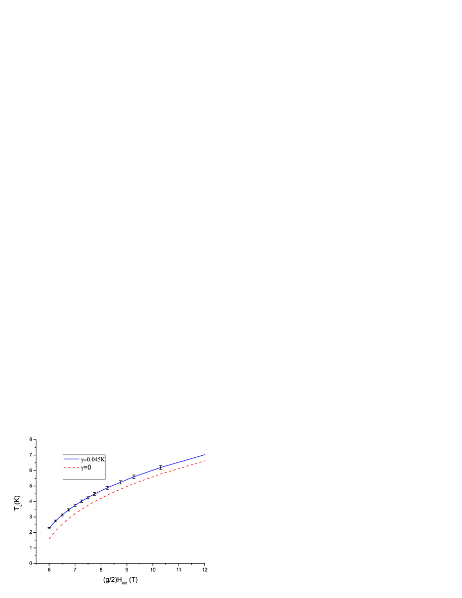
a)

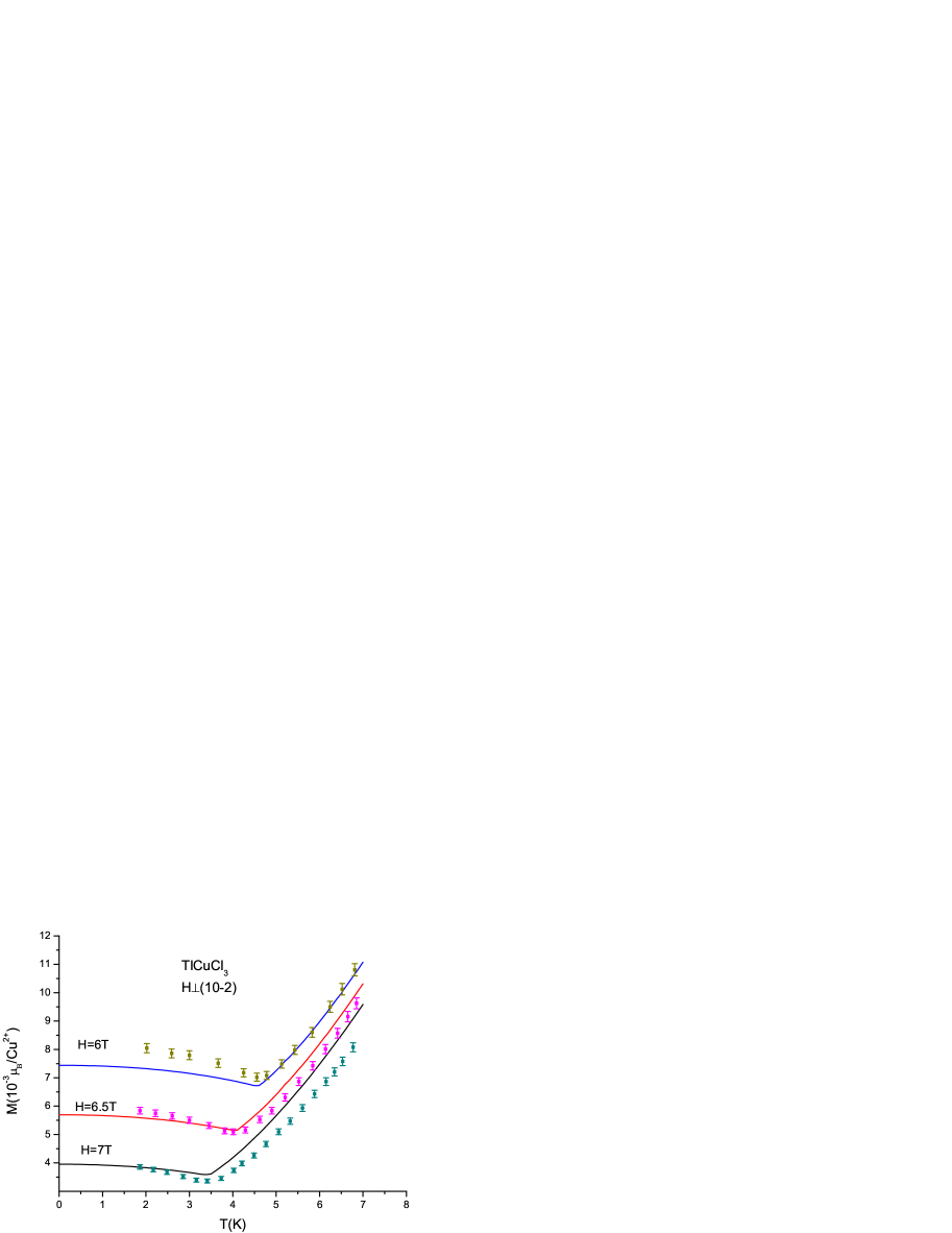
b)

Figure 1: Phase diagram normalized by the g-factor (a) and low- temperature magnetization curves (b) for TlCuCl₃ . The experimental data are taken from [5]. The input parameters are $\gamma=0.045\rm{K}$, $c_{\gamma}$=1.67 , U=367.52K , g=2.23 and $\Delta_{\rm{st}}=7.54\rm{K}$ for our HFB approximation

The phase boundary $T_{c}(H_{\rm{ext}})$, displayed in Fig.1 (a), is intersting by itself, since it contains information about the critical exponent $\phi$, defined as $T_{c}\sim(H_{\rm{ext}}-H_{c})^{\phi}$ or more precisely as $T_{c}=\rm{const}\times(\mu/U)^{\phi}$, where the constant and $\phi$ are fitting parameters. Note that for the case of a homogeneous ideal gas with the quadratic dispersion $\phi=2/3$. From Fig.1(a) we have found that $\rm{const}=47.4\rm{K}$ and $\phi=0.53$ (solid line) and $\rm{const}=63.2\rm{K}$ and $\phi=0.62$ (dashed line) for the $\gamma=0.045\rm{K}$ and $\gamma=0$ cases respectively. This means that the inclusion of a finite exchange anisotropy reduces the exponent $\phi$, and one does not need to expect $\phi=2/3$ as it has been debated in the literature [31, 30, 32]. In fact, the presence of the interparticle interaction as well as using a more realistic dispersion than a simple quadratic one, leads to a shift of the critical temperature, especially at high temperatures $T>2\rm{K}$ [33]. Here we note that, if we restrict to fit $\phi$ in the range of $0\leq T\leq 1.5\rm{K}$ (not drawn in Fig.1a ) the solid line in Fig.1 (a) may also be well fitted by $\phi\approx 2/3.$

In Fig. 1(b) the magnetization curves for various $H_{\rm{ext}}$ are presented in comparison with the experimental data from Ref. [5] for $H_{\rm{ext}}\perp(1,0,$2̄$)$ . It is seen that, by taking into account the exchange anisotropy one can obtain an excellent agreement with the experimental data. This result is in quite contrast to the results from Sirker et al. [13] that were based on the HFP approximation alone.

The optimized parameters $\gamma$ and U are universal for both $H$$\perp$(1,0,2̄) and $H$$\parallel$b cases. The main difference is only in the g-factors. Using in the above equations $g=2.06$ we also obtain the total magnetization for $H$$\parallel$b, which is plotted in Fig.2(a) in comparison with the experimental data taken from [6] and with a corresponding calculaions based on the HFP approximations [13]. It is seen that by neglecting the anomalous density $\sigma$ (dashed line) or the exchange anisotropy , $\gamma$, (dotted line) one may reproduce the experimental magnetization only at high temperatures , $T>T_{c}$, while the inclusion of both, $\sigma$ and $\gamma$ makes it possible to obtain a significantly better theoretical description (solid line) for $T\leq T_{c}$ also. From the Fig. 2(a) one may conclude that the effect of the exchange anisotropy is rather large in the BEC - like phase and is almost negligible in the normal phase.

Another important characteristics of quantum magnets is that the magnetically ordered state supports a staggered magnetization $M_{\perp}$ transverse to the field direction, leading to a canted antiferromagnetic state until the system becomes eventually fully polarized as the external field increases. In the BEC- scenario the number of triplons corresponds to the total magnetization $M_{z}$ along the field direction, while the number of condensed particles is proportional to the square of the ordered transverse component:

$$M_{\perp}=N_{f}g\mu_{B}\sqrt{\rho_{0}/2},$$ (57blbtbu)

where $N_{f}$ is a normalization factor [6]. In our present approximation $M_{\perp}$ may be calculated directly from Eqs. (49)-(52) and (57blbtbu). The results are presented in Fig.2 (b), where we have used the same input parameters as in Figs.1 and chosen the scaling factor $N_{f}=6.5$ to reproduce the experimental data [34]. As it is seen from the figure the present approach with exchange anisotropy describes well the experimental data for $T\leq T_{c}$. A comparison of the dotted curve with the solid line in Fig. 2(b) shows that the exchange anisotropy enhances the staggered magnetization.

In the vicinity of the critical point the staggered magnetization scales as $M_{\perp}\sim(T_{c}-T)^{\beta}$, ($T\leq T_{c}$) defining the critical exponent $\beta$. Approximating the curves in Fig. 2(b) as

$$M_{\perp}=\rm{const}\times(1-T/T_{c})^{\beta},$$ (57blbtbv)

we have found $\beta=0.47$ in the present approximation, which is close to the predictions made in Quantum Monte Carlo simulations [35]: $\beta_{QMC}=1/2$. The other curves in Fig.2 (b) lead to $\beta=0.15$ and $\beta=0.39$ for HFP and HFB with $\gamma=0$ cases, respectively.

In the present work we have been dealing only with the exchange anisotropy, which gives a sharp phase transition with $\rho_{0}(T\geq T_{c})=0$. Comparing our magnetization curves for the total magnetization with the experimental data (see Fig.1(b) and Fig. 2(a)) we may conclude that including a finite exchange anisotropy is sufficient. However, as it has been shown by Sirker et al. the inclusion of a DM anisotropy instead may lead to a crossover [13], so that $M_{\perp}^{\rm{DM}}(T\geq T_{c})\neq 0$. Indeed, from the fact that experimental data on the tranverse magnetization show $M_{\perp}^{\rm{exp}}(T\geq T_{c})\neq 0$, (see Fig. 2(b) with data from Fig.3 in Ref. [34]) one may conclude that a certain DM anisotropy is clearly present. Moreover, Density Matrix Renormalization Group calculations [36] show that even a tiny DM interaction can modify some aspects of the physics, especially the staggered magnetization, rather dramatically. We shall develop a HFB approximation including both exchange and DM anisotropies in a subsequent publication and do not discuss it here any further.

From Fig. 1(a) we can state that the exchange anisotropy term $H^{\prime}_{\rm{EA}}$ given in (5) leads to an increase of the critical temperature at a given magnetic field. To study this issue in more detail we present in Fig. 3(a) the shift of the critical temperature due to the anisotropy $\Delta T/T_{c}^{0}$ vs $\gamma$ for various values of $H_{\rm{ext}}$. We see that

• $\Delta T_{c}$ increases with the increase of $\gamma$;

• For a moderate value of gamma $\gamma\sim 0.04\rm{K}$ the shift is nearly $10\%$ at $H_{\rm{ext}}=7\rm{T}$;

• With increasing the magnetic field, the upward shift in the critical temperature decreases.

A similar dependence of the shift on $\gamma$ and $H_{\rm{ext}}$ has been predicted by Dell’Amore et al. [12].

There is another effect due to the explicit $U(1)$ - symmetry breaking. In real systems the presence of an anisotropy modifies the energy dispersion of the magnetic excitations. Experimentally, the excitation spectrum of TlCuCl₃ was investigated by Rüegg et al. [4] using INS measurements. In the frame of Bogolyubov mean field theory this spectrum coincides with spectrum of quasiparticles (called as bogolons) which can be calculated from equation (47) in the present approximation. The energy dispersion of the low- lying magnetic excitations measured for $H$_ext=14T at temperatures $T$=50mK and $T$=1.5 K are presented in Fig.3(b), where the solid line is obtained in the HFB approximation (47) using our optimized parameters. It can be seen that the agreement with the experiment is satisfactory, especially at small momentum transfer. Clearly in the BEC phase without anisotropy the energy dispersion is linear at small momentum, i.e. $E_{k\rightarrow 0}(H_{\rm{ext}},T,\gamma=0)\sim ck$ , (with c is the sound velocity), while the presence of an anisotropy causes a gap $\Delta E=E_{k\rightarrow 0}(H_{\rm{ext}},T,\gamma)\neq 0$ which can be calculated directly from Eq. (47). The average sound velocity at small momentum defined as $c=(\partial E/\partial k)\mid_{k\rightarrow 0}$ is given by $c(\gamma=0)=\sqrt{X_{1}/2m}$ at $T\leq T_{c}$ and $c(\gamma\neq 0)=k(X_{1}+X_{2})/2m\sqrt{X_{1}X_{2}}$ at any temperature, where $m$ is the effective mass [30] and $X_{1},X_{2}$ are given by Eq. (28). Fig. 3(c) illustrates the fact that, being zero at $\gamma=0$, the gap in the quasiparticle spectrum increases with $\gamma$. In the present approach, $\Delta E=E_{k\rightarrow 0}(H_{\rm{ext}}=14\rm{T},T=1.5\rm{K},\gamma=0.045\rm{K})=0.7\rm{K}$ which is the detection limit of Ref. [4].

A possible modification of the spin gap separating the singlet ground state from the lowest - energy triplet excitation $\Delta_{\rm{st}}$ due the anisotropy, is not considered here, and we used the experimental value $\Delta_{\rm{st}}=7.55\rm{K}$ [30] (see appendix A).

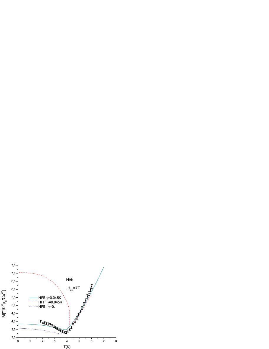
a)

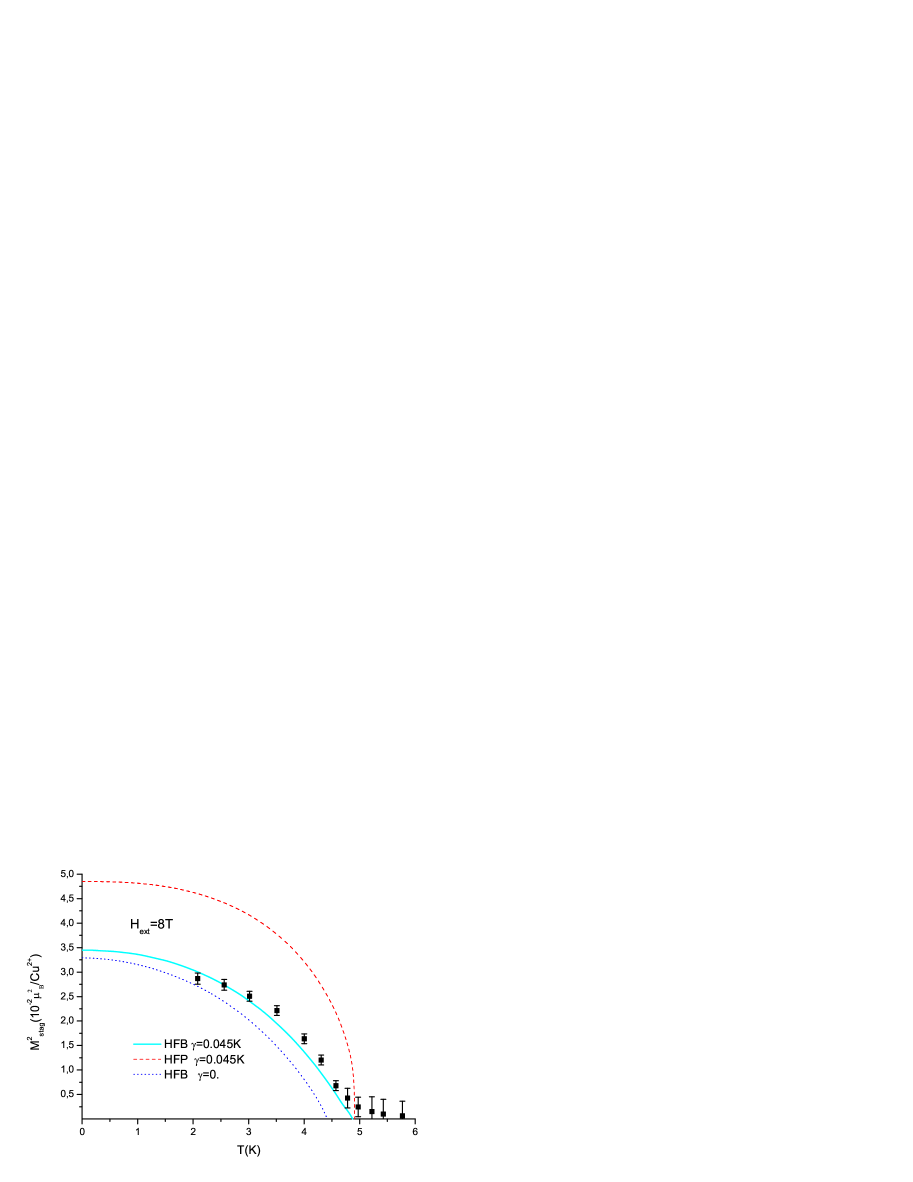
b)

Figure 2: The total magnetization (a) and square of the transverse magnetization (b) in different approximations for $H\|b$. The solid and dashed lines are for HFB and HFP apppoximations with the exchange anisotropy and the same input parameters, respectively. The dashed line in (a) is reproduced from Ref. [13] and the experimental data are taken from [6, 34]. The dotted line represents a HFB approximation without anisotropy, i.e. $\gamma=0$, and $U=367.5\rm{K}$

Finally we discuss the role of the anomalous density whose absolute value is the density of pair correlated particles. This pair correlations are, actually, responsible for the existence of superfluidity [21]. We present in Fig.4(a) the density of condensed particles $\rho_{0}$ (solid line) and the absolute value of the anomalous density $\mid\sigma\mid$ (dashed line) versus the reduced temperature. It is seen that $\mid\sigma\mid$ is comparable with $\rho_{0}$ at all temperatures. Another interesting fact, which is demonstrated in Fig. 4(b) is that the anomalous density surives, although on a small level, even above the critical temperature where it vanishes asypmtotically. For example, $\sigma(t=0)/\sigma(t=1)\approx 100$. Note that without exchange anisotropy $\sigma(\gamma=0)\mid_{T\geq T_{c}}=0$. A similar phase with $\rho_{0}=0$ and $\sigma\neq 0$ has been reported by Cooper et al. [37] within a lowest - order auxiliary field formalism. In fact, this approach predicts the existence of two critical temperatures, one $T_{c}$, where $\rho_{0}=0$, $\sigma\neq 0$ and another one $T^{*}$, where $\rho_{0}=0$, $\sigma=0$, with $T^{*}>T_{c}$. This exotic state in the region $T_{c}<T<T^{*}$ has not been experimentally observed yet, but it is predidicted to exhibit a modified dispersion relation. The question about the observing such phase still remains open.

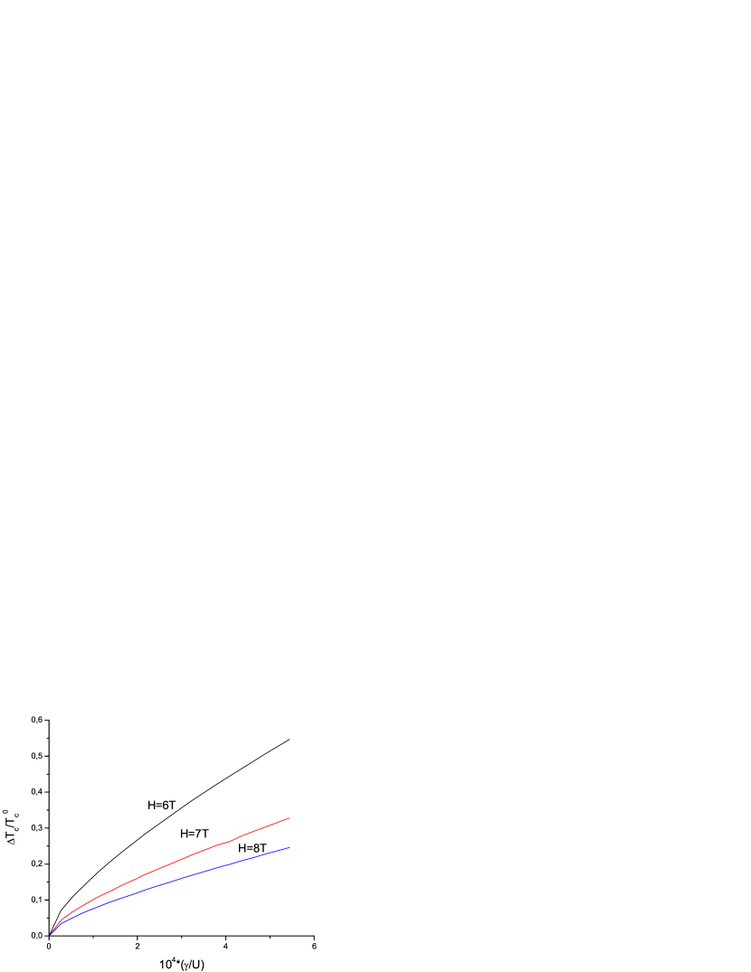
a)

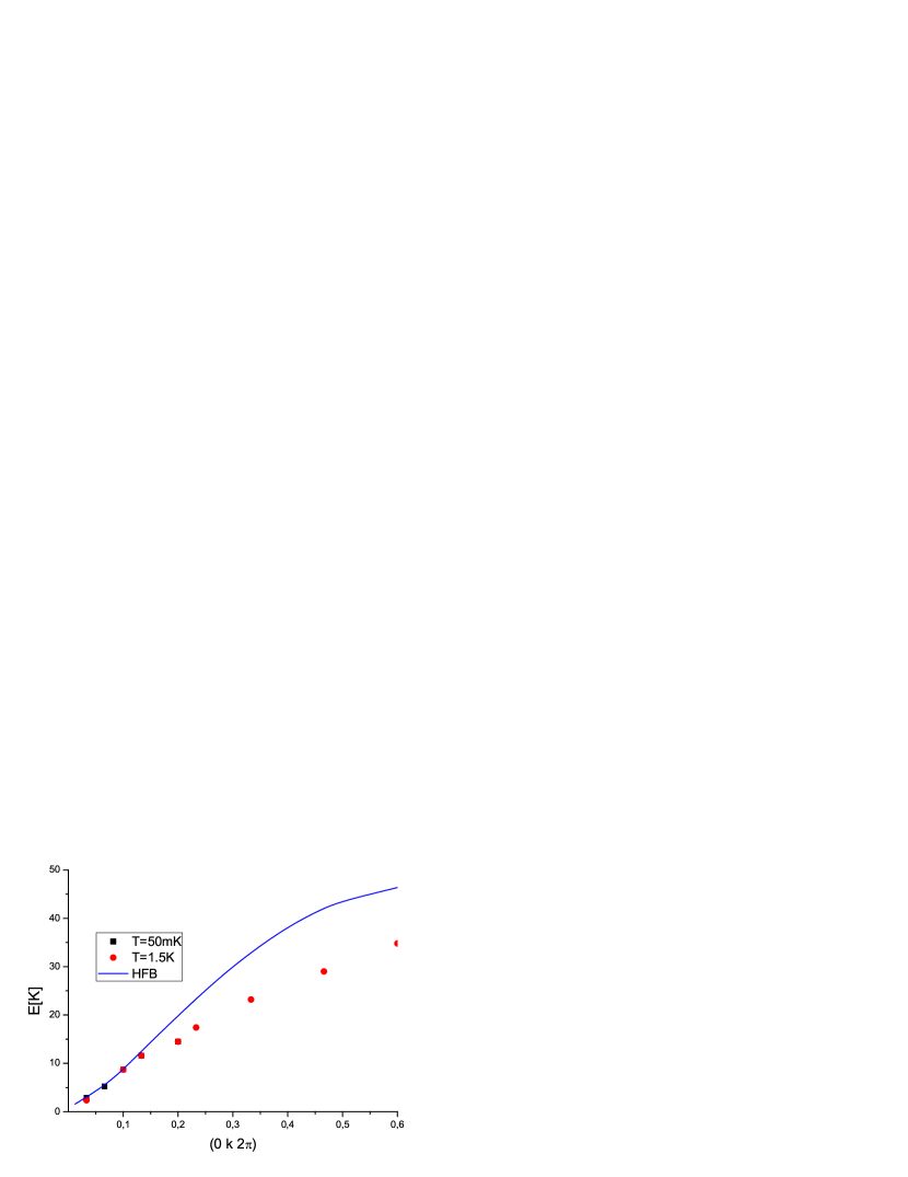
b)

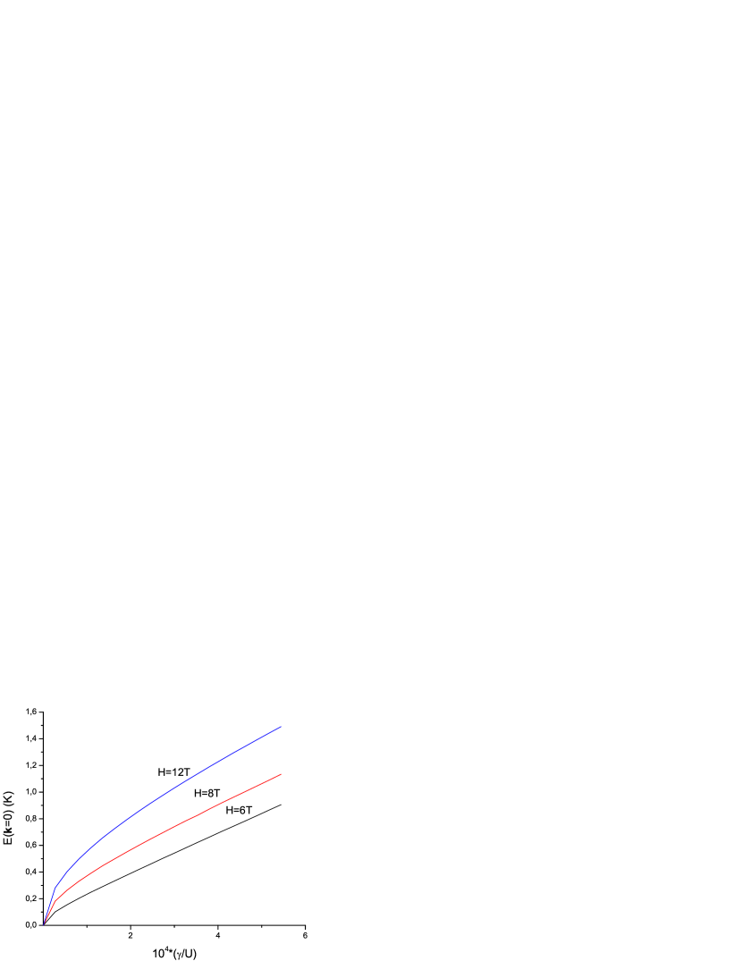
c)

Figure 3: (a): The shift of the critical temperature, $(T_{c}(\gamma)-T_{c}(\gamma=0))/T_{c}(\gamma=0)$ due to the anisotropy ; (b): Quasiparticle spectrum (solid line) (47) in HFB approximation with the optimized parametrs for $H=14\rm{T}$ at $T\leq 1.5\rm{K}$ . INS data for $T=50\rm{mK}$ (circles) and $T=1.5\rm{K}$ (squares) taken from Ref. [4] are shown for comparision. (c): The collective excitation gap $E_{k=0}$ in Eq. (47) in the BEC phase vs. $\gamma$ at $T$=1.5 K.;.

.

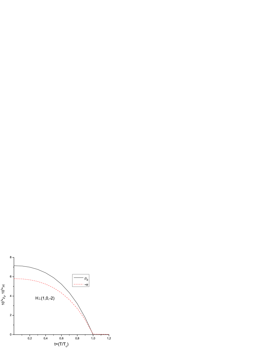
a)

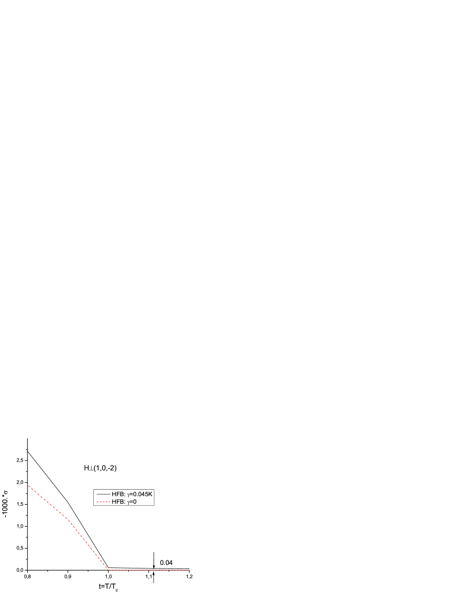
b)

Figure 4: (a): The condensed (solid line) and the absolute value of anomalous densities (dashed line) in HFB approximation at $H_{\rm{ext}}=7\rm{T}$; (b): The behavior of $\mid\sigma(t)\mid$ near the critical temperature with (solid line) and without (dashed line) exchange anisotropy.

.

5 Conclusion

Assuming that the low temperature properties of quantum magnets with a weak $U(1)$ symmetry breaking can be described in a BEC - like scenario, we proposed a new MFA based approach within the Hartree - Fock - Bogolyubov approximation, which takes into account an anomalous density $\sigma$ and exchange anisotropy. This approach not only reproduces experimental data such as the critical temperature and the magnetization in a satisfactory way, but also removes certain inconsistencies and drawbacks met in the previous Hartree - Fock - Popov approaches [13]. Remarkably, this may be reached by optimizing only three paramters : $\gamma$- the parameter of the exchange anisotropy, $c_{\gamma}$- the parameter of breaking of the Hugenholtz – Pines relation and U - the interparticle interaction. We have found $\gamma=0.045\rm{K}=0.0038\rm{meV}$, $c_{\gamma}=1.67$ and $U=367.5\rm{K}$ valid for both $H{\parallel}b$ and $H\perp(1,0,\bar{2})$ directions.

The present approach also gives a fair theoretical description of the staggered magnetization data for $T\leq T_{c}$ and predicts a plausible value for the critical exponent $\beta$. However, to improve the theoretical description of the experimental data on staggered magnetization the inclusion of Dzyaloshinsky-Moriya anisotropy also seems to be nessesary. We have estimated the anisotropy - induced shift of the critical temperature, and show that it is substantial. Finally, we predict that the anomalous density is comparable to the condensded one, and survives at temperatures exceeding $T_{c}$ where the condensate fraction is zero.

Appendix A

The summation by momentums may be explicitly written as

$$\sum_{\mathbf{k}}f(\varepsilon(k))=\frac{1}{{(2\pi)^{3}}}\left\{\begin{array}[]{ll}{4\pi}\int\limits_{0}^{\infty}k^{2}dkf(\varepsilon(k)),\quad\varepsilon(k)=\frac{k^{2}}{2m}\quad,&\hbox{}\\ \int\limits_{-\pi}^{\pi}dk_{x}dk_{y}dk_{z}f(\varepsilon(k)),\quad\varepsilon(k)-\textrm{isotropic}\quad,&\hbox{}\\ \frac{1}{2}\int\limits_{-\pi}^{\pi}dk_{x}\int\limits_{-\pi}^{\pi}dk_{y}\int\limits_{-2\pi}^{2\pi}dk_{z}\varepsilon(k),\quad(\varepsilon(k))-\textrm{realistic, anisotropic}.&\hbox{}\end{array}\right.$$ (A.4)

The isotropic bare dispersion may be presented as $\varepsilon(k)=J[3-\cos k_{x}a-\cos k_{y}a-\cos k_{z}a]$ where $a$ is the size of the unit cell ( below we set $a=1$), while the anisotropic one may be written as [30]

$$\begin{array}[]{l}\varepsilon_{k-k_{0}}=-\Delta_{st}+\sqrt{(J+\tilde{a})^{2}-\tilde{a}^{2}},\\ \tilde{a}=J_{a}\cos(k_{x})+J_{a2c}\cos(2k_{x}+k_{z})+2J_{abc}\cos(k_{x}+k_{z}/2)\cos(k_{y}/2).\end{array}$$ (A.5)

In practical calculations with this realistic dispersion one may make a shift as $\mathbf{k}-\mathbf{k}_{0}\rightarrow\mathbf{k}$, so that $\varepsilon(k-k_{0})|_{k=k_{0}}\rightarrow\varepsilon(k)|_{k=0}=0$, $k_{0}=\{0,0,2\pi\}$ and introducing $q_{x}=k_{x}/\pi$, $q_{y}=k_{y}/\pi$, $q_{z}=k_{z}/4\pi$ we can rewrite the summation as

$$\sum_{\mathbf{k}}f(\varepsilon(k))|_{aniz}=\frac{1}{2}\int\limits_{-1}^{1}dq_{x}\int\limits_{0}^{1}dq_{y}\int\limits_{0}^{1}dq_{z}f(\varepsilon(q)),$$ (A.6)

where $\varepsilon_{q}=-\Delta_{st}+\sqrt{J^{2}+2Ja_{q}}$, and

$$a_{q}=J_{a}\cos(\pi q_{x})+J_{a2c}\cos(2\pi q_{x}-4\pi q_{z})-2J_{abc}\cos(\pi q_{x}-2\pi q_{z})\cos(\pi q_{y}/2).$$ (A.7)

The condition $\varepsilon_{q}(q=0)=0$ fixes $\Delta_{st}$ as $\Delta_{st}=\sqrt{J^{2}+2J(J_{a}+J_{a2c}-2J_{abc})}$. In the present work we used the following values of parameters [30]: $J=63.7$K, $J_{a}=-2.5K$, $J_{a2c}=-18.35$K and $J_{abc}=5.28K$, so that $\Delta_{st}=7.55K$.

Appendix B

In the notion of representative ensemble [21] the grand Hamiltonian including the exchange anisotropy term can be written as:

$$\begin{array}[]{l}H=\hat{H}-\mu_{0}\hat{N}_{0}-\mu_{1}\hat{N}_{1}-\hat{\Lambda},\\ \hat{H}=\int\left\{\psi^{{\dagger}}(\mathbf{r})\hat{K}\psi(\mathbf{r})+\frac{U}{2}\left(\psi^{{\dagger}}(\mathbf{r})\psi(\mathbf{r})\right)^{2}+\frac{{\gamma}}{2}\left(\psi^{{\dagger}}(\mathbf{r})\psi^{{\dagger}}(\mathbf{r})+\psi(\mathbf{r})\psi(\mathbf{r})\right)\right\}d^{3}r,\end{array}$$ (B.1)

where $\hat{N}_{0}=\int\mid\phi_{0}\mid^{2}d^{3}r$,  $\hat{N}_{1}=\int\widetilde{\psi}^{{\dagger}}(\mathbf{r})\widetilde{\psi}(\mathbf{r})d^{3}r$,  so that $\mu N=\mu_{0}N_{0}-\mu_{1}N_{1}$, $\hat{N}=\int\psi^{{\dagger}}\psi d^{3}r$   is the total number of particles. The Lagrange multiplier

$$\hat{\Lambda}=\int[\lambda\widetilde{\psi}^{{\dagger}}(\mathbf{r})+\lambda^{{\dagger}}\widetilde{\psi}(\mathbf{r})]d^{3}r$$ (B.2)

is a so called linear killer, such that $\lambda$ is chosen from the constraint for the conservation of quantum numbers, $\langle\widetilde{\psi}(\mathbf{r})\rangle=0$. The quantum fluctuation $\widetilde{\psi}(\mathbf{r})$ is related to the field operator as $\psi(\mathbf{r})=\phi_{0}+\widetilde{\psi}(\mathbf{r})$, which makes possible to rewrite the grand Hamiltonian as follows:

$$H=H_{0}+H_{1}+H_{2}+H_{3}+H_{4},$$ (B.3)

where

$$H_{0}=\int d^{3}r\rho_{0}(-\mu_{0}+\gamma+\frac{U}{2}\rho_{0})$$ (B.4)

with $\rho_{0}=\phi_{0}^{2}$

$$H_{1}=\int d^{3}r\phi_{0}(\gamma+U\rho_{0})(\widetilde{\psi}^{{\dagger}}(\mathbf{r})+\widetilde{\psi}(\mathbf{r})),$$ (B.5)

$$H_{2}=\int d^{3}r\left\{\widetilde{\psi}^{{\dagger}}(\mathbf{r})[\hat{K}-\mu_{1}+2U\rho_{0}]\widetilde{\psi}(\mathbf{r})+\frac{1}{2}\left(\widetilde{\psi}^{2}(\mathbf{r})+\widetilde{\psi}^{{\dagger}2}(\mathbf{r})\right)({\gamma}+U\rho_{0})\right\},$$ (B.6)

$$H_{3}=U\phi_{0}\int d^{3}r\widetilde{\psi}^{{\dagger}}(\mathbf{r})\widetilde{\psi}(\mathbf{r})\left(\widetilde{\psi}^{{\dagger}}(\mathbf{r})+\widetilde{\psi}(\mathbf{r})\right),$$ (B.7)

$$H_{4}=\frac{U}{2}\int d^{3}r(\widetilde{\psi}^{{\dagger}}(\mathbf{r})\widetilde{\psi}(\mathbf{r}))^{2}.$$ (B.8)

Performing a Fourier transformation $\widetilde{\psi}(\mathbf{r})=\sum_{\mathbf{k}\neq 0}a_{\mathbf{k}}\widetilde{\psi}_{\mathbf{k}}(\mathbf{r})$ and assuming that $\phi_{0}(\mathbf{r})$ does not depend on ${\mathbf{r}}$ we may rewrite the above equations as follows:

$$\begin{array}[]{l}H_{0}=\rho_{0}(-\mu_{0}+\gamma+\frac{U}{2}\rho_{0}),\\ H_{1}=\sqrt{\rho_{0}}(U\rho_{0}+\gamma)\sum_{\mathbf{k}}(a_{\mathbf{k}}+a_{\mathbf{k}}^{{\dagger}}),\\ H_{2}=\sum_{\mathbf{k}}\{\varepsilon_{k}-\mu_{1}+2U\rho_{0}\}a_{\mathbf{k}}^{{\dagger}}a_{\mathbf{k}}+\frac{1}{2}(a_{\mathbf{k}}a_{-\mathbf{k}}+a_{\mathbf{k}}^{{\dagger}}a_{-\mathbf{k}}^{{\dagger}})({U\rho_{0}+\gamma}),\\ H_{3}=U\sqrt{\rho_{0}}\sum_{\mathbf{k},\mathbf{p}}(a_{\mathbf{k}}^{{\dagger}}a_{\mathbf{k}+\mathbf{p}}a_{-\mathbf{p}}+\rm{h.c.}),\\ H_{4}=\displaystyle{\frac{U}{2}}\sum_{\mathbf{k},\mathbf{q},\mathbf{p}}a_{\mathbf{k}}^{{\dagger}}a_{\mathbf{p}}^{{\dagger}}a_{\mathbf{p}+\mathbf{q}}a_{\mathbf{k}-\mathbf{q}}.\end{array}$$ (B.9)

The third and fourth order terms may be further simplified by using the approximation given in Eq. (17) as:

$$\begin{array}[]{l}H_{3}=U\sqrt{\rho_{0}}(2\rho_{1}+\sigma)\sum_{\mathbf{k}}(a_{\mathbf{k}}^{{\dagger}}+a_{\mathbf{k}}),\\ H_{4}=\displaystyle{\frac{U}{2}}\{4\rho_{1}a_{\mathbf{k}}^{{\dagger}}a_{\mathbf{k}}+\sigma(a_{\mathbf{k}}a_{-\mathbf{k}}+a_{-\mathbf{k}}^{{\dagger}}a_{\mathbf{k}}^{{\dagger}})-(2\rho_{1}^{2}+{\sigma}^{2})\}.\end{array}$$ (B.10)

Now the grand Hamiltonian is the sum of classical, $H_{\rm{class}}$, linear $H_{\rm{lin}}$ and $H_{\rm{bilin}}$ terms as:

$$\begin{array}[]{l}H=H_{\rm{class}}+H_{\rm{lin}}+H_{\rm{bilin}},\\ H_{\rm{class}}=-\rho_{0}\mu_{0}+\rho_{0}\gamma+\displaystyle{\frac{U}{2}}\rho_{0}^{2}-\displaystyle{\frac{U}{2}}(2\rho_{1}^{2}+{\sigma}^{2}),\\ H_{\rm{lin}}=U\sqrt{\rho_{0}}(\rho_{0}+\widetilde{\gamma}+2\rho_{1}+\sigma)\sum_{\mathbf{k}}(a_{\mathbf{k}}^{{\dagger}}+a_{\mathbf{k}}),\\ H_{\rm{bilin}}=\sum_{\mathbf{k}}(\varepsilon_{k}-\mu_{1}+2U\rho)a_{\mathbf{k}}^{{\dagger}}a_{\mathbf{k}}+\displaystyle{\frac{U({\rho_{0}+\widetilde{\gamma}+\sigma})}{2}}\sum_{\mathbf{k}}(a_{\mathbf{k}}a_{-\mathbf{k}}+a_{\mathbf{k}}^{{\dagger}}a_{-\mathbf{k}}^{{\dagger}}),\end{array}$$ (B.11)

where $\widetilde{\gamma}=\gamma/U$ and $\rho=\rho_{0}+\rho_{1}$. In the formalism of representative ensemble [21] the linear term is neglected by an appropriate choice of $\lambda$, for example, by choosing $\lambda=U\sqrt{\rho_{0}}(\rho_{0}+\widetilde{\gamma}+2\rho_{1}+\sigma)$ in Eq. (B.2). The $\mu_{0}$ can be found by minimization of the free energy with respect to $\rho_{0}$. To diagonalize the bilinear term we introduce the normal $\Sigma_{n}$ and anomalous $\Sigma_{an}$ self energies as

$$\begin{array}[]{l}\Sigma_{n}=2U\rho,\\ \Sigma_{an}=U(\rho_{0}+\widetilde{\gamma}+\sigma),\end{array}$$ (B.12)

such that $H_{\rm{bilin}}$ is rewritten as

$$H_{\rm{bilin}}=\sum_{\mathbf{k}}\omega_{k}a_{\mathbf{k}}^{{\dagger}}a_{\mathbf{k}}+\frac{\Sigma_{an}}{2}\sum_{\mathbf{k}}(a_{\mathbf{k}}a_{-\mathbf{k}}+a_{\mathbf{k}}^{{\dagger}}a_{-\mathbf{k}}^{{\dagger}}),$$ (B.13)

where

$$\omega_{k}=\varepsilon_{k}-\mu_{1}+\Sigma_{n}.$$ (B.14)

The next step is the Bogolyubov transformation

$$a_{\mathbf{k}}=u_{\mathbf{k}}b_{\mathbf{k}}+v_{\mathbf{k}}b_{-{\mathbf{k}}}^{\dagger},\quad a_{\mathbf{k}}^{\dagger}=u_{\mathbf{k}}b_{\mathbf{k}}^{\dagger}+v_{\mathbf{k}}b_{-{\mathbf{k}}}$$ (B.15)

to diagonalize ${H}_{\rm{bilin}}$. The operators $b_{\mathbf{k}}$ and $b_{\mathbf{k}}^{\dagger}$ can be interpreted as annihilation and creation operators of phonons with following properties:

$$[b_{\mathbf{k}},b_{\mathbf{p}}^{\dagger}]=\delta_{\mathbf{k},\mathbf{p}},\quad\langle b_{\mathbf{k}}^{\dagger}b_{-{\mathbf{k}}}^{\dagger}\rangle=\langle b_{\mathbf{k}}b_{-\mathbf{k}}\rangle=0,$$ (B.16)

$$\langle b_{\mathbf{k}}^{\dagger}b_{\mathbf{k}}\rangle=f_{B}(E_{k})=\displaystyle\frac{1}{e^{\beta E_{k}}-1},$$ (B.17)

where $\beta\equiv 1/T$. To determine the phonon dispersion $E_{k}$ we insert (B.15) into (B.13) and require that the coefficient of the term $b_{\mathbf{k}}b_{-\mathbf{k}}+b_{-\mathbf{k}}^{\dagger}b_{\mathbf{k}}^{\dagger}$ vanishes, i.e:

$$\omega_{k}u_{\mathbf{k}}v_{\mathbf{k}}+\frac{\Sigma_{an}}{2}\left(u^{2}_{\mathbf{k}}+v_{\mathbf{k}}^{2}\right)=0.$$ (B.18)

Now using the condition $u_{\mathbf{k}}^{2}-v_{\mathbf{k}}^{2}=1$ and presenting $u_{\mathbf{k}},v_{\mathbf{k}}$ as

$$u_{\mathbf{k}}^{2}=\frac{\omega_{k}+E_{k}}{2E_{k}},\quad\quad v_{\mathbf{k}}^{2}=\frac{\omega_{k}-E_{k}}{2E_{k}}$$ (B.19)

yields

$$\sqrt{\omega_{k}^{2}-E_{k}^{2}}=-\Sigma_{an},\quad\quad u_{\mathbf{k}}v_{\mathbf{k}}=-\frac{\Sigma_{an}}{2E_{k}},\quad\quad u_{\mathbf{k}}^{2}+v_{\mathbf{k}}^{2}=\frac{\omega_{k}}{E_{k}}$$ (B.20)

that is

$$\begin{array}[]{l}E_{k}^{2}=(\omega_{k}+\Sigma_{an})(\omega_{k}-\Sigma_{an})\equiv(\varepsilon_{k}+X_{1})(\varepsilon_{k}+X_{2})\end{array}$$ (B.21)

with

$$\left\{\begin{array}[]{ll}X_{1}=\Sigma_{n}+\Sigma_{an}-\mu_{1}&\hbox{}\\ X_{2}=\Sigma_{n}-\Sigma_{an}-\mu_{1}&\hbox{}.\end{array}\right.$$ (B.24)

Now $H_{\rm{bilin}}$ is simplified as

$$H_{\rm{bilin}}=\sum_{\mathbf{k}}E_{k}b_{\mathbf{k}}^{{\dagger}}b_{\mathbf{k}}+\frac{1}{2}\sum_{\mathbf{k}}(E_{k}-\omega_{k})$$ (B.25)

and the total Hamiltonian is given by

$$H=H_{\rm{class}}+H_{\rm{bilin}}=-\rho_{0}\mu_{0}+\rho_{0}\gamma+\frac{U}{2}\rho_{0}^{2}-\frac{U}{2}(2\rho_{1}^{2}+{\sigma}^{2})+\sum_{\mathbf{k}}E_{k}b_{\mathbf{k}}^{{\dagger}}b_{\mathbf{k}}+\frac{1}{2}\sum_{\mathbf{k}}(E_{k}-\omega_{k})$$ (B.26)

which may be used to define the energy of the system.

Note that by requiring in (B.21) $X_{2}=0$, one may directly obtain from Eqs. (B.24) the Hugenholtz - Pines theorem as well as the gapless dispersion in SSB phase. The main Eqs. (40) and (41) are derived by inserting (B.24) into (B.12). The normal and anomalous densities may be obtained by using Eqs. (B.15) in Eqs. (18) and (19) leading to the expressions (30) and (31) respectively, where $X_{1}$ and $X_{2}$ are given in (B.24) and (B.12).

References

References

- [1] Cheng T.P. and Li L.F. 1988 Gauge theory of elementary particle physics (Oxford University Press).
- [2] Ginibre J. Commun. Math.Phys. 1968 8 26
- [3] Oosawa A. et al. 1999 J. Phys. Condens. Matter 11 265
- [4] Rüegg Ch. et al. 2003 Nature (London) 423 62
- [5] Yamada F. et al. 2008 J. Phys. Soc. Jpn. 77 013701
- [6] Nikuni T. et al. 2000 Phys. Rev. Lett. 84 5868
- [7] V. Yukalov 2012 Laser Physics 22 1145
- [8] Zapf V. and Jaime M. 2014 Rev.Mod.Phys 86 563
- [9] Čižmár E. et al. 2010 Phys Rev. B 82 054431
- [10] Rüegg Ch. et al. 2008 Phys. Rev. Lett. 100 205701
- [11] Giamarchi T. et al. 2008 Nat. Phys. 4 198
- [12] Dell Amore R., Schilling A. and Krämer K. 2009 Phys. Rev. B 79 014438
- [13] Sirker J., Weisse A., and Sushkov O. P. 2004 Europhys. Lett. 68 275
- [14] Rakhimov A. , Sherman E. Ya., and Kim Chul Koo 2010 Phys. Rev. B 81 020407(R)
- [15] Rakhimov A. , Mardonov S. , and Sherman E. Ya. 2011 Ann. Phys. 326 2499
- [16] Dodds T. Yang B., and Kim Y. 2010 Phys. Rev. B 81 054412
- [17] Hohenberg P.C. and Martin P. 1965 Ann. Phys. 34 291
- [18] Hugenholtz N. M. and Pines D. 1959 Phys. Rev. 116 489
- [19] Yukalov V. I. and Kleinert H. 2006 Phys. Rev. A 73 063612
- [20] Rakhimov A. et al. 2012 New J. Phys. 14 113010
- [21] Yukalov V. I. 2011 Physics of Particles and Nuclei 42 460
- [22] Kleinert H., Schmidt S. , and Pelster A. 2005 Annalen der Physik (Leipzig) 14 214 .
- [23] Andersen J. 2004 Rev. Mod. Phys. 76 599
- [24] Yukalov V.I. and Yukalova E.P. 2005 Laser Phys. Lett. 2 506
- [25] Yukalov V. I., Rakhimov A. , and Mardonov S. 2011 Laser Physics 2 264
- [26] Stoof H. T. C., Gubbels K. B. and Dickerscheid D.B.M. 2009 Ultracold Quantum Fields (Springer)
- [27] Kleinert H., Narzikulov Z. and Rakhimov A. 2012 Phys. Rev. A 85 063602
- [28] Griffin A. 1996 Phys. Rev. B 53 9341
- [29] Dell Amore R., Schilling A. and Krmer K. 2008 Phys. Rev. B 78 224403
- [30] Misguich G. and Oshikawa M. 2004 J. Phys. Soc. Jpn. 73 3429
- [31] Sherman E.Ya. et al. 2003 Phys. Rev. Lett. 91 057201 .
- [32] Yamada F. 2011 et al. Phys. Rev. B 83 020409(R)
- [33] Kastening B. 2003 Phys. Rev. A68 061601
- [34] Tanaka H. et al. 2001 J. Phys. Soc. Jpn. 70 939
- [35] Nohadani O., Wessel S. and Haas S. 2005 Phys. Rev. B 72 024440
- [36] Miyahara S. et al. 2007 Phys. Rev. B 75 184402
- [37] Cooper F. 2011 et al. Phys. Rev. A 83 053622