Surface Ocean Enstrophy, Kinetic Energy Fluxes and Spectra from Satellite Altimetry

Abstract

Enstrophy, kinetic energy (KE) fluxes and spectra are estimated in different parts of the mid-latitudinal oceans via altimetry data. To begin with, using geostrophic currents derived from sea-surface height anomaly data provided by AVISO, we confirm the presence of a strong inverse flux of surface KE at scales larger than approximately 250 km. We then compute enstrophy fluxes to help develop a clearer picture of the underlying dynamics at smaller scales, i.e., 250 km to 100 km. Here, we observe a robust enstrophy cascading regime, wherein the enstrophy shows a large forward flux and the KE spectra follow an approximate $k^{-3.5}$ power-law. Given the rotational character of the flow, not only is this large scale inverse KE and smaller scale forward enstrophy transfer scenario consistent with expectations from idealized studies of three-dimensional rapidly-rotating and strongly-stratified turbulence, it also agrees with detailed analyses of spectra and fluxes in the upper level midlatitude troposphere. Decomposing the currents into components with greater and less than 100 day variability (referred to as seasonal and eddy, respectively), we find that, in addition to the eddy-eddy contribution, the seasonal-eddy and seasonal-seasonal fluxes play a significant role in the inverse (forward) flux of KE (enstrophy) at scales larger (smaller) than about 250 km. Taken together, we suspect, it is quite possible that, from about 250 km to 100 km, the altimeter is capturing the relatively steep portion of a surface oceanic counterpart of the upper tropospheric Nastrom-Gage spectrum.

I Introduction

For the past decade, satellite altimetry data has been used to estimate the interscale transfer and spectral distribution of surface kinetic energy, henceforth abbreviated as KE, in the oceans. Focusing on mesoscales in mid-latitudinal regions with high eddy activity (for example, near the Gulf Stream, the Kuroshio or the Agulhas currents), the flux of KE is seen to be scale dependent. In particular, it has been noted that surface KE tends to be transferred upscale for scales larger than the local deformation radius and downscale for smaller scales (Scott and Wang, 2005; Tulloch et al., 2011; Arbic et al., 2014, 2012). Mesoscale wavenumber spectra, on the other hand, are somewhat more diverse with spectral indices ranging from $-\frac{5}{3}$ to $-3$ depending on the region in consideration (Stammer, 1997; Le Traon et al., 2008; Xu and Fu, 2012). In fact, recent work using in-situ observations suggests that the scaling changes with season, and is modulated by the strength of eddy activity (Callies et al., 2015). Interpreting these results in terms of the dynamics captured by the altimeter and more fundamentally the nature of the actual dynamics of the upper ocean has been the subject of numerous recent investigations (see for example the discussions in, Lapeyre, 2009; Ferrari and Wunsch, 2010).

As baroclinic modes are intensified near the surface (Wunsch, 1997; Smith and Vallis, 2001), it has been suggested that altimetry data mostly represents the first baroclinic mode in the ocean (Stammer, 1997). Indeed, energy is expected to concentrate in the first baroclinic mode due to an inverse transfer among the vertical modes (Fu and Flierl, 1980). Given this, at first sight, the observed inverse transfer of surface KE at large scales was surprising, as classical quasigeostrophic (QG) baroclinic turbulence anticipates a forward cascade in the baroclinic mode with energy flowing towards the deformation scale (Salmon, 1980; Hoyer and Sadourny, 1982). However, a careful examination of the energy budget in numerical simulations reveals that, while KE goes to larger scales, the total energy in the first baroclinic mode does indeed flow downscale (Scott and Arbic, 2007); a feature that is comforting in the context of traditional theory. In fact, along with the two-layer QG study of Scott and Arbic (2007), inverse transfer of KE has also been documented in more comprehensive ocean models (Schlösser and Eden, 2007; Venaille et al., 2011; Arbic et al., 2012, 2014).

Noting the significance of surface buoyancy gradients (a fact missed in the aforementioned first baroclinic mode framework), it has been suggested that, surface QG (SQG) dynamics is a more appropriate framework for the oceans’ surface (Lapeyre and Klein, 2006), and is reflected in the altimeter measurements (Lapeyre, 2009). Even though the variance of buoyancy is transferred downscale (Pierrehumbert et al., 1994; Sukhatme and Pierrehumbert, 2002), surface KE actually flows upscale in SQG dynamics (Smith et al., 2002; Capet et al., 2008), consistent with the flux calculations using altimetry data. Of course, in the QG limit, a combination of surface and interior modes is only natural. There are ongoing efforts to represent the variability of the surface ocean and interpret the altimetry data in these terms (Lapeyre, 2009; Scott and Furnival, 2012; Smith and Vanneste, 2013).

Thus, much of the work using altimeter data has focussed on the inverse transfer of KE at relatively large scales. Here, we spend some time on the larger scales, but mainly concentrate on slightly smaller scales that are still properly resolved by the data. Specifically, in addition to the KE flux, we also compute the spectral flux of enstrophy. In fact, this enstrophy flux sheds new light on the range of scales that span approximately 250 km to 100 km. We find that the enstrophy flux is strong and directed to small scales over this range, and is accompanied by a KE spectrum that follows an approximate $k^{-3.5}$ power-law. This suggests that the rotational currents as derived from the altimeter are in an enstrophy cascading regime from about 250 km to 100 km, and in an inverse KE transfer regime for scales greater than about 250 km. In terms of an eddy and slowly varying or seasonal decomposition (defined as smaller and larger than 100 day timescale variability, respectively), we observe that the seasonal-seasonal and seasonal-eddy fluxes play a significant role in the KE (enstrophy) flux for scales larger (smaller) that about 250 km. Finally, we interpret these findings in the context of idealized studies of three-dimensional, rapidly rotating and stratified turbulence and also compare them with detailed analyses of midlatitude upper tropospheric KE spectra and fluxes.

II Data Analysis and Methodology

II.1 Data Description

Gridded data of sea-surface height (SSH) anomalies (MADT delay time gridded data) from the AVISO project has been used in our analysis. The data spanning 21 years (1993-2013) is available at a spatial resolution of $0.25^{\circ}\times 0.25^{\circ}$, thus scales smaller than approximately 50 km can not be resolved. We compute horizontal currents from the SSH anomaly data using geostrophic balance relations, and the latitudinal variation of the Coriolis parameter has been included in the computations.

II.2 Geographical Locations

The five geographical regions chosen for analysis are located far from the equator so that geostrophic balance is expected to be dominant. As is seen in Figure 1, these regions represent relatively uninterrupted stretches in the Northern and Southern parts of the Pacific, Atlantic, and the Southern Indian Ocean. In essence, we expect that this choice of domain minimizes boundary effects. Region 1 is the largest which is about 4500 km long and 3500 km wide. Other regions are comparatively smaller.

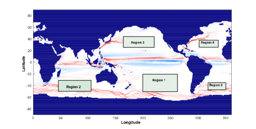
Figure 1: Regions 1-5 chosen for the analysis. These are centered at $-36^{\circ}$, $232^{\circ}$ (grid size $256\times 128$); $-38^{\circ}$, $78^{\circ}$ (grid size $256\times 64$); $33^{\circ}$, $187^{\circ}$ (grid size $256\times 64$); $30^{\circ}$, $316^{\circ}$ (grid size $128\times 64$) and $-42^{\circ}$, $336^{\circ}$ (grid size $128\times 64$), respectively.

II.3 Computation of Spectra and Fluxes

In this paper, we compute the KE spectrum and fluxes of KE and enstrophy. For this purpose, the data is represented using Fourier modes in both spatial directions, i.e.,

$${{\bf U}}({\bf k})=\int\!\!\!\int{\bf U}(x,y)\exp[-{\rm i}(k_{x}x+k_{y}y)]dxdy,$$ (1)

where, ${\bf k}=(k_{x},k_{y})$ and ${\bf U}=(u,v)$ contains the zonal and meridional components of the velocity. The two-dimensional (2D) Fourier transform technique requires the data to have uniform grid spacing in both directions, so a linear interpolation scheme is employed to generate the velocity data on a rectangular grid (the original data is on equidistant latitudes and longitudes). In order to make the velocity field spatially periodic, the data is multiplied with a 2D bump function ($\exp[{-\frac{0.01}{1-x^{2}}-\frac{0.01}{1-y^{2}}+0.02}]$ where $(x,y)\in[-1,1]$) before performing a Fourier transform, this ensures that the velocity smoothly goes to zero at the boundaries.

In Fourier space, the KE equation is represented as (Scott and Wang, 2005),

$$\frac{\partial E(k)}{\partial t}=T(k)+F(k)-D(k),$$ (2)

where $E(k)$ is the KE of a shell of wavenumber $k=\sqrt{k^{2}_{x}+k^{2}_{y}}$, $F(k)$ is the energy supply rate to the above shell by forcing, and $D(k)$ is the energy dissipation at the shell. $T(k)$ is the energy supply to this shell via nonlinear transfer. Note that,

$$E(k)=\frac{1}{2}\!\!\sum_{k-1<|k^{\prime}|\leq k}\!\!\!\!\!\!\!\!\!|{{\bf U}}({\bf k}^{\prime})|^{2}.$$ (3)

In a statistically steady state, $\partial E(k)/\partial t=0$, and $E(k)$ is approximately constant in time. The energy supply rate due to non-linearity is balanced by $F(k)-D(k)$. A useful quantity called the KE flux, $\Pi(k)$, measures the energy passing through a wavenumber of radius $k$, and it is defined as,

$$\Pi(k)=-\int_{0}^{k}T(k^{\prime})dk^{\prime}.$$ (4)

In 2D flows, another quantity of interest is the enstrophy ($\zeta=\int\!\frac{\omega^{2}}{2}d{\bf r}$), where $\omega$ is the relative vorticity. The corresponding enstrophy flux is denoted by $\zeta(k)$. We compute the KE and enstrophy fluxes using the formalism of Dar et al. (2001) and Verma (2004), and the relevant formulae read,

$$\Pi(k)=\sum_{k^{\prime}>k}\sum_{p\leq k}\delta_{\bf{k^{\prime}},\bf{p}+\bf{q}}Im([\bf{k^{\prime}\cdot U(q)}][\bf{U^{*}(k^{\prime})\cdot U(p)}]),$$ (5)

$$\zeta(k)=\sum_{k^{\prime}>k}\sum_{p\leq k}\delta_{\bf{k^{\prime}},\bf{p}+\bf{q}}Im([\bf{k^{\prime}\cdot U(q)}][\omega^{*}(\bf{k^{\prime}})\omega(\bf{p})]),$$ (6)

where $Im$ stands for the imaginary part of the argument and $\bf{U}^{*}$ is the complex conjugate. The expression (inside the summation operators) in equation 5 (6) represents the energy (enstrophy) transfer in a triad (${\bf{k^{\prime}}}={\bf{p}}+{\bf{q}}$) where $\bf{k^{\prime}}$ mode receives energy (enstrophy) from modes $\bf{p}$ and $\bf{q}$. Then, the expression is integrated over all such possible triads satisfying the condition $k^{\prime}>k$ and $p\leq k$ (note that $-\int_{0}^{k}T(k^{\prime})dk^{\prime}$ = $\int_{k}^{\infty}T(k^{\prime})dk^{\prime}$).

III Results

We begin by considering the spectra and fluxes associated with daily geostrophic currents. Figure 2 shows KE spectra of the geostrophic currents derived from SSH anomalies in all five regions. As seen, these currents show an approximate $k^{-3.5}$ scaling (the best fits range from $k^{-3.5}$ to $k^{-3.6}$) over a range of 250 to 100 km in all regions except Region 1 (the Southern Pacific), where the slope is somewhat shallower with a best fit of $k^{-2.9}$. Thus, the spectra we obtain for geostrophic currents are more in line with those reported by Stammer (1997), Scharffenberg and Stammer (2011) (global extratropics), Arbic et al. (2014) (Agulhas region) and Wang et al. (2010) & Callies and Ferrari (2013) (near the Gulf Stream), but differ from the shallower $-\frac{5}{3}$ like scaling observed by Le Traon et al. (2008) (see also Xu and Fu, 2012).

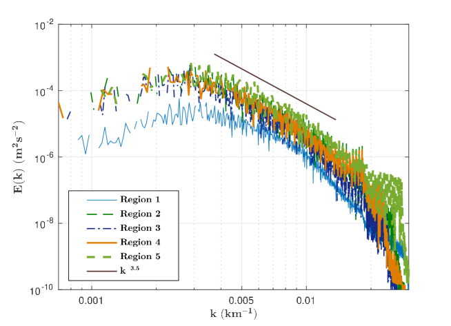
Figure 2: Surface KE spectra for the geostrophic currents (averaged over 21 years of data). The slopes obtained between wavenumbers 0.004 and 0.01 (i.e., 250 km to 100 km) are: $-2.85,-3.54,-3.48,-3.71$ and $-3.61$ for regions 1-5 respectively.

The KE and enstrophy fluxes are shown in Figure 3. Note that we have computed the flux using daily data and the results presented are an average over the entire 21 year period. The qualitative structure of the KE flux confirms the findings of Scott and Wang (2005) (see also Scott and Arbic, 2007; Tulloch et al., 2011; Arbic et al., 2014). Specifically, we observe a robust inverse transfer of KE at large scales (i.e., greater than approximately 250 km). Some regions (1 and 2) show a very weak forward transfer of KE at small scales, while in the others (Region 3, 4 and 5), the flux continues to be negative (though very small in magnitude) even at small scales. In fact, in all the regions considered, the KE flux crosses zero or becomes very small by about 200 km. Note that $2\pi$ times the climatological first baroclinic deformation scale in these five regions also lies between 200 and 250 km (Chelton et al., 1998). Whether this is indicative of a KE injection scale due to linear instability as put forth by Scott and Wang (2005), or more of a coincidence is not particularly clear. Indeed, a mismatch between the deformation and zero-crossing scale can be seen in Tulloch et al. (2011) and has also been pointed out by Schlösser and Eden (2007) in a comprehensive ocean model.

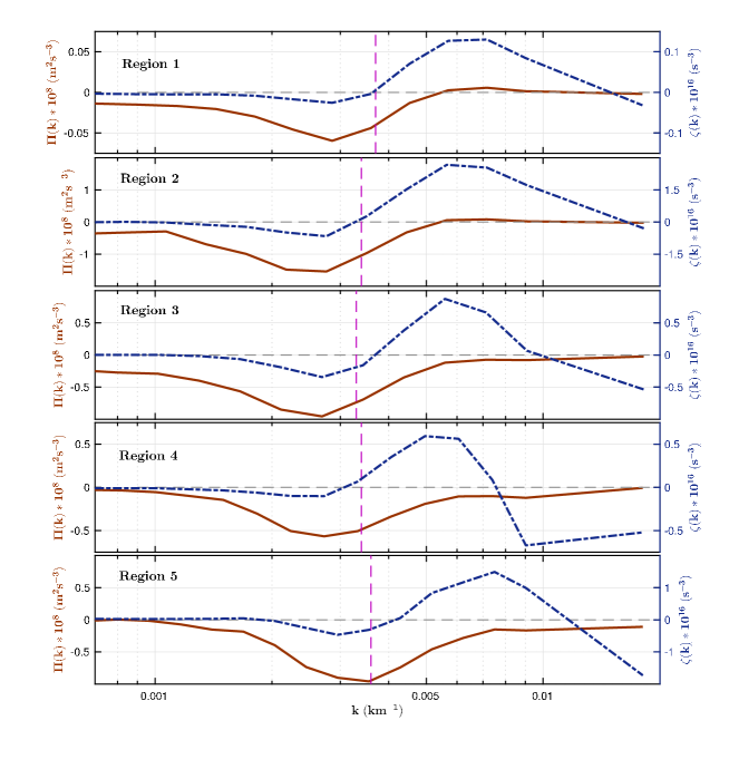
Figure 3: KE (solid) and enstrophy (dash) fluxes for geostrophic currents (averaged over all 21 years) vs wavenumber ($k^{2}$ = $k^{2}_{x}$ + $k^{2}_{y}$). Vertical dashed lines mark the transition scale ($\sqrt{\langle E\rangle/\langle\zeta\rangle}$) in each region.

Proceeding to the enstrophy, also shown in Figure 3, we see that it is characterized by a large forward flux at scales smaller than approximately 250 km. Further, the enstrophy flux does not show an inertial range, rather it increases with progressively smaller scales and peaks at approximately 150 km. Interestingly, we note that, in most of the regions, the scale $\sqrt{\langle E\rangle/\langle\zeta\rangle}$ (where $\langle\cdot\rangle$ denotes a domain average) (Danilov and Gurarie, 2000) — shown by the dashed vertical lines in Figure 3 — serves as a reasonable marker for the onset of the forward enstrophy flux regime.

III.1 Eddy (subseasonal) and slowly varying (seasonal) fluxes

An important difference between actual geophysical flows (the atmosphere and ocean) and idealized 3D rotating stratified turbulence is the presence of nontrivial mean flows, and a hierarchy of prominent temporal scales. To get an idea of the KE and enstrophy flux contributions from the fast and slowly-varying components of the flow, following Shepherd (1987), we filter the derived geostrophic currents. In particular, at every grid point, we consider the daily 21 year long time series and split this into two parts: one that contains variability of less than 100 days (referred to as the eddy or transient component) and the other with only larger than 100 day timescales (referred to as the slowly varying, or for brevity, as the seasonal component). To get a feel for the physical character of the these decompositions, Figures 4 and 5 we show a snapshot of the zonal and meridional velocities (during summer) for all of the five regions. Quite clearly, the slowly varying or seasonal $u$ flow has a pronounced zonal structure, as compared to the more isotropic eddy component. Similarly, the seasonal $v$ velocity has a larger scale and is oriented in a preferentially meridional direction as compared to its eddy component. It is interesting to note that the meridional (seasonal and eddy) velocity is always comparable in strength to the zonal flow.

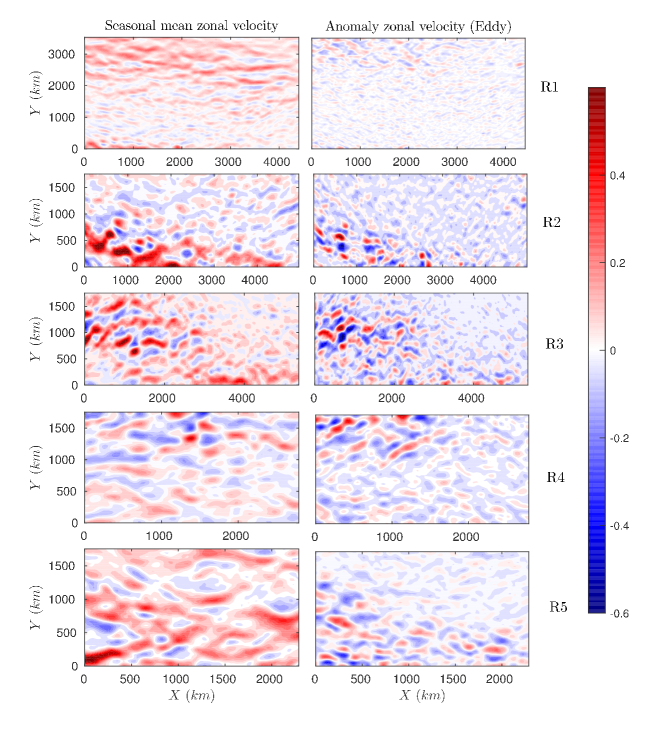
Figure 4: Snapshot of the zonal seasonal and eddy fields in the summer (specifically on 16th June, 2005). R1-R5 correspond to Region1-Region5 of Figure 1.

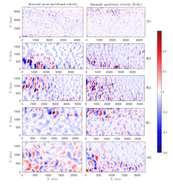
Figure 5: Snapshot of the meridional seasonal and eddy fields in the summer (specifically on 16th June, 2005). R1-R5 correspond to Region1-Region5 of Figure 1.

As with the original data (the total field), we compute the KE and enstrophy fluxes from the eddy field and the seasonal component. The seasonal-eddy fluxes are computed by subtracting the eddy-eddy and seasonal-seasonal contributions from the total flux. Figures 6 and 7 show these four terms (total: solid curves, eddy-eddy: dashed curves, seasonal-seasonal: dotted curves and seasonal-eddy: dash-dot curves) for KE and enstrophy in the five regions considered, respectively. For the KE (Figure 6), we see that the total flux at large scales (i.e., greater than 250 km) has a strong contribution from the seasonal-eddy interactions. In fact, the eddy-eddy term is qualitatively of the correct form but quite small in magnitude. The seasonal-seasonal contribution is always upscale (except for a very small positive bump at small scales in Region 1), and thus, it too enhances the inverse transfer at large scales. For the enstrophy (Figure 7), we see that the eddy-eddy term is reasonably strong, and along with the seasonal-eddy flux (in Regions 3,4 and 5), or the seasonal-seasonal flux (in Region 1), or both (Region 2) leads to the strong forward enstrophy cascading regime at small scales (i.e., below approximately 250 km).

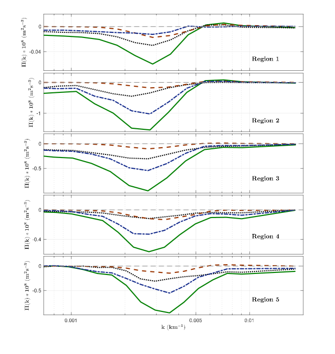
Figure 6: Total (solid), eddy-eddy (dash), slowly varying-slowly varying (dot) and slowly varying-eddy (dash-dot) KE fluxes for geostrophic currents (averaged over all 21 years) vs wavenumber ($k=\sqrt{k_{x}^{2}+k^{2}}$) in all the five regions regions.

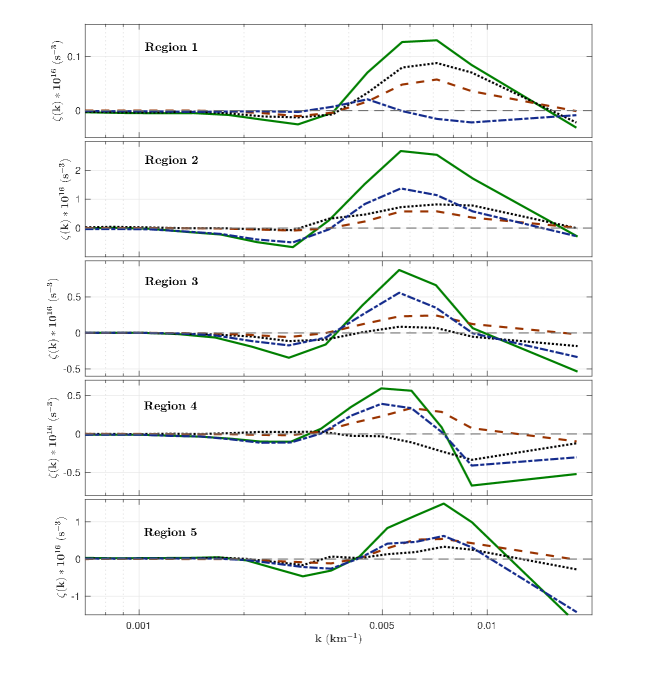
Figure 7: Total (solid), eddy-eddy (dash), slowly varying-slowly varying (dot) and slowly varying-eddy (dash-dot) enstrophy fluxes for geostrophic currents (averaged over all 21 years) vs wavenumber ($k=\sqrt{k_{x}^{2}+k^{2}}$) in all the five regions regions.

IV Interpretation and Conclusion

By studying 21 years (1993-2013) of surface geostrophic currents derived from AVISO SSH anomalies in different midlatitudinal parts of the world’s oceans we find — in agreement with previous studies — that the spectral flux of rotational KE exhibits an inverse transfer at scales larger than about 250 km. Further, at smaller scales, specifically, 250 km to 100 km, we find a strong forward flux of enstrophy accompanied by a KE spectrum that approximately follows a $k^{-3.5}$ power-law. The KE flux at these small scales is very weak, and in a few of the regions considered, it is in the forward direction. The transition from an inverse KE to a dominant forward enstrophy flux is roughly in agreement with a simple prescription based on the total enstrophy and KE in the domain. On splitting the original data into high (eddy) and low (seasonal) frequencies, we observed that the seasonal-seasonal and seasonal-eddy fluxes play an important role in the inverse (forward) transfer of KE (enstrophy) at scales greater (smaller) than 250 km. We now interpret these findings in the context of rapidly rotating, strongly stratified three-dimensional (3D) turbulence as well as spectra and flux analyses from the midlatitude upper troposphere.

Specifically, idealized 3D rotating Boussinesq simulations suggest that rotational (or vortical) modes dominate the energy budget at large scales and exhibit a robust inverse transfer of KE to larger scales, and a forward transfer of enstrophy to small scales (Bartello, 1995; Kitamura and Matsuda, 2006; Sukhatme and Smith, 2008; Vallgren et al., 2011). These transfers, akin to 2D and QG turbulence, are accompanied by KE spectra that follow $-\frac{5}{3}$ and $-3$ power-laws in the upscale KE and downscale enstrophy flux dominated regimes (Kraichnan, 1967; Charney, 1971). Given the rotational nature of the geostrophic currents, our observation of the upscale (downscale) KE (enstrophy) flux at scales greater (smaller) than 250 km is therefore in accord with the aforementioned expectations. Indeed, the $k^{-3.5}$ scaling is also close to the expected KE spectrum that characterizes the enstrophy flux dominated regime .

With regard to the atmosphere, the forward enstrophy transfer regime of QG turbulence has been postulated to explain the $-3$ portion of midlatitude upper tropospheric KE spectrum (the so-called Nastrom-Gage spectrum, Nastrom and Gage, 1985). Starting with Boer and Shepherd (1983) and Shepherd (1987), re-analysis products at progressively finer resolutions have been analyzed with a view towards seeing if the Nastrom-Gage spectrum is captured by the respective models (see for example, Strauss and Ditlevsen, 1999; Koshyk and Hamilton, 2001; Hamilton et al., 2008), and if so, what are the associated energy and enstrophy fluxes that go along with it (Augier and Lindborg, 2013; Burgess et al., 2013). In all, these studies demonstrate quite clearly that the $-3$ range of the Nastrom-Gage spectrum (spanning approximately 3000-4000 km to 500 km in the upper troposphere) corresponds to the dominance of rotational modes, and a forward enstrophy cascading regime. Further, at scales greater than the $-3$ range (i.e., greater than approximately 4000 km), the upper troposphere supports an inverse rotational KE flux (Augier and Lindborg, 2013; Burgess et al., 2013).

Regarding the small forward flux of rotational KE at scales smaller than approximately 250 km in a few regions, as pointed out by Boer and Shepherd (1983) and Burgess et al. (2013), this is likely due to the limited resolution of the data. For example, a forward KE flux in the rotational modes was observed in the coarse data used by Boer and Shepherd (1983), but it vanishes in the more recent finer scale products analyzed in Augier and Lindborg (2013) and Burgess et al. (2013) (see, Boffetta, 2007, for similar issues in incompressible 2D turbulence). In fact, much like the idealized 3D rotating stratified scenario (Bartello, 1995; Kitamura and Matsuda, 2006; Sukhatme and Smith, 2008), the forward transfer of KE at small scales in atmospheric data (i.e., below approximately 500 km and accompanied by a shallower KE spectrum) is likely due to the divergent component of the flow (Augier and Lindborg, 2013; Burgess et al., 2013).

On decomposing the flow into eddy and seasonal components (less and greater than 100 day timescales, respectively), our results are somewhat analogous to the upper troposphere. Specifically, in the atmosphere, the zonal mean-eddy (which translates to a stationary-eddy or seasonal-eddy decomposition) flux enhanced the inverse KE transfer to large scales (Shepherd, 1987; Burgess et al., 2013). We find the seasonal-eddy term to be important, but the seasonal-seasonal contribution to also be significant in the inverse transfer. In fact, in our decomposition (based on a timescale of 100 days), these terms dominate over the eddy-eddy contribution. For enstrophy, in the upper troposphere, Shepherd (1987) noted that the stationary-eddy fluxes are important (as we do here), but higher resolution data employed in Burgess et al. (2013) suggests that the eddy-eddy term is the dominant contributor to the forward enstrophy flux.

Thus our findings using altimeter data, i.e., employing purely rotational geostrophic currents, are in fair accordance with expectations from idealized simulations of rotating stratified flows as well as analyses of upper tropospheric re-analysis data. The qualitative similarity in rotational KE fluxes, enstrophy fluxes, and KE spectra between the surface ocean currents and the near tropopause atmospheric flow is comforting as they both are examples of rapidly-rotating and strongly-stratified fluids. In fact, in addition to an inverse rotational KE flux at large scales, we believe it is quite possible that the altimeter data is showing us an enstrophy cascading, and relatively steep spectral KE scaling range of a surface oceanic counterpart to the atmospheric Nastrom-Gage spectrum. Quite naturally, it would be very interesting to obtain data at a finer scale, and see if the ocean surface currents (rotational and divergent together) also exhibit a transition to shallower spectra — like the upper tropospheric Nastrom-Gage spectrum — with a change in scaling at a length scale smaller than 100 km.