Beyond Evolutionary Algorithms for Search-based Software Engineering

Abstract

Context: Evolutionary algorithms typically require large number of evaluations (of solutions) to converge – which can be very slow and expensive to evaluate.

Objective: To solve search-based software engineering (SE) problems, using fewer evaluations than evolutionary methods.

Method: Instead of mutating a small population, we build a very large initial population which is then culled using a recursive bi-clustering chop approach. We evaluate this approach on multiple SE models, unconstrained as well as constrained, and compare its performance with standard evolutionary algorithms.

Results: Using just a few evaluations (under 100), we can obtain comparable results to state-of-the-art evolutionary algorithms.

Conclusion: Just because something works, and is widespread use, does not necessarily mean that there is no value in seeking methods to improve that method. Before undertaking search-based SE optimization tasks using traditional EAs, it is recommended to try other techniques, like those explored here, to obtain the same results with fewer evaluations.

shadows

1 Introduction

Due to the complexities of software architectures and shareholder requirements, it is often hard to solve complex modeling problems via a standard numerical mathematical analysis or some deterministic algorithms [25]. There are many reasons for this complexity:

• When procedural code is used within the model of a domain, every “if” statement can divide the internal problem space into different regions (once for each branch in the “if”). Such software models cannot be optimized via traditional numerical methods which assume models are a single continuous differentiable function.

• Finding solutions to problems often means accommodating competing choices. When stakeholders propose multiple goals, search-based SE (SBSE) methods can reflect on goal interactions to propose novel solutions to hard optimization problems such as configuring products in complex product lines [54], tuning parameters of a data miner [59], or finding best configurations for clone detection algorithms [63].

For these tasks, many SBSE researchers usually use evolutionary algorithms (EA) [54, 59, 63]. Evolutionary algorithms start by generating a set of initial solutions and improve them through crossover and mutation, also known as reproduction operators. They are inspired by evolution in nature and make no parametric assumptions about problems being generated. In our experience, this has made them particularly well-suited for SE problems. However, evolutionary algorithms typically require large number of evaluations (of solutions) to converge. Real-world model-based applications may be very expensive to evaluate (with respect to computation time, resources required etc.).

So, can we do better than EA for SBSE? Or, are there faster alternatives to EA? This paper experimentally evaluates one such alternative called SWAY (short for the Sampling WAY):

1. Similar to a standard EA, generate an initial population;

2. Intelligently select a cluster within the population generated with best scores.

SWAY runs so fast since it terminates after just $O(lgN)$ evaluations of $N$ candidate solutions. SWAY’s intelligent selection mechanism for exploring subsets of the population is a recursive binary chop that (i) finds and evaluates only the two most dissimilar examples, then (ii) recurses only on half of the data containing the better among its similar example. As shown later in this paper, for this process to work, it is important to have the right definition of “dissimilar”.

Note the differences between SWAY and standard EA:

1. SWAY quits after the initial generation while EA reasons over multiple generations;

2. SWAY makes no use of reproduction operators so there is no way for lessons learned to accumulate as it executes;

3. Depending on the algorithm, not all members of the population will be evaluated – e.g. active learners [34] only evaluate a few representative individuals.

Because of the limited nature of this search, until recently, we would have dismissed SWAY as comparatively less effective than EA for exploring multi-goal optimization. Nevertheless, quite by accident, we have stumbled onto evidence that has dramatically changed our opinion about SWAY. Recently we were working with an algorithm called GALE [34]. GALE is an evolutionary algorithm that includes SWAY as a sub-routine:

$$\begin{array}[]{rcl}\textit{evolution}&=&\textit{generations}*\left\{\begin{array}[]{l}\textit{mutation}\\ \textit{crossover}\\ \textit{sampling}\\ \end{array}\right.\\ \textit{SWAY}&=&\textit{GALE}-\textit{evolution}\\ \end{array}$$

While porting GALE from Python to Java, we accidentally disabled evolution. To our surprise, the “broken” version worked as well, or better, than the original GALE. This is an interesting result since GALE has been compared against dozens of models in a recent TSE article [34] and dozens more in Krall’s Ph.D. thesis [31]. In those studies, GALE was found to be competitive against widely used evolutionary algorithms. If Krall’s work is combined with the results from our accident, then we conjecture that the success of GALE is due less to “evolution” than to “sampling” many options. This, in turn, could lead to a new generation of very fast optimizers since, as we show below, sampling can be much faster than evolving.

The rest of this paper describes SWAY and presents evidence for its utility. While we have tested SWAY on the standard EA benchmarks such as DTLZ, Fonseca, Golinski, Srinivas, etc. [16], those results are not included here since, in our experience, results from those benchmarks are less convincing to the SE community than results from software models. Hence, here we present results from:

• POM3: a model of agile teams selecting their next task from the scrum backlog [51, 9];

• XOMO: a model predicting software development time, effort, risks and defects [41, 45, 44];

• MONRP: a model of next release planning that recommends which functionality to code next [4].

After presenting some background motivational notes, this paper offers general notes on multi-objective evolutionary algorithms. This is followed by a description of SWAY and the POM3, XOMO, MONRP models. Experimental results are then presented showing that SWAY achieves results competitive with standard methods (NSGA-II and SPEA2) using orders of magnitude fewer evaluations. Working with the MONRP models, we also find that a seemingly minor detail (the implementation of the distance function used to recognize “dissimilar” examples) is of vital importance to the success of SWAY. Finally, this paper concludes with experiments on “super-charging” that tests whether SWAY can boost the performance of standard optimizers.

Our observations after conducting the study are:

• The mutation strategies seen in a recently published EA algorithm (GALE) adds little value;

• GALE without evolution (SWAY) runs an order of magnitude faster than EAs;

• Optimization found by SWAY are similar to those found by SBSE algorithms;

• How we recognize “dissimilar” examples is of vital importance;

• Super-charging (combining SWAY with standard SBSE optimizers) is not useful.

More generally, our conclusion is that sampling is an interesting research approach for multi-dimensional optimization that deserves further attention by the SBSE community.

1.1 Connection to Prior Work

This paper significantly extends prior work by the authors. The background notes in the next section are new to the paper, as is the super-charging study. Also, this paper repairs a significant drawback seen in initial describing of SWAY. At SSBSE’16 [48], we demonstrated how SWAY can be used to find near optimal solutions for problems like XOMO and POM. While an interesting result, it turns out that the early definition of “dissimilar” used by the earlier version of SWAY was only applicable to problems whose decision space is constrained in nature. The results on other types of problems, were less than impressive. In this paper, we expose the weakness of the earlier variant of SWAY and show other definitions of “dissimilar” can make SWAY very useful for other domains.

1.2 When is SWAY most Useful, Useless?

SWAY is designed as a fast substitution of EAs for solving SBSE problems. It can avoid large amount of model evaluations, which are very common in previous evolutionary algorithms. In view of this, SWAY is particularly useful in following two scenarios.

SWAY would be most useful if it is proposed to put humans-in-the-loop to help guide the evaluations (e.g. as done in [53]). In this scenario, standard EAs might have to ask a human for up to $O(N^{2})$ opinions for $G$ generations. On the other hand, SWAY would only trouble the user $O(lgN)$ times

Also, SWAY was created to solve problems, where the practitioner is not able to evaluate thousands of individuals for e.g. Wang et al. [64] spent 15 years of CPU time to find software clone detectors or model explored by Krall et al. [34]) which take hours to perform a single evaluation.

However, as discussed later in this paper, SWAY has two core assumptions. Firstly, it is applicable only when there is a mapping between “genotype” and “phenotype” space; i.e. between the settings to the model inputs and outputs of the model. Even though such mapping may not exist in every model, we find here that for SE models (that were written with the explicit goal of effecting outputs with input decisions), this assumption holds adequately, at least for the purposes of improving model output.

Secondly, SWAY techniques for dividing the data makes the spectral learning assumption; i.e. that within the raw dimensions of data seen in any domain, there exists a small set of spectral dimensions which can usefully approximate the larger set [28]. While the universality of the spectral assumption has not been proven, it has seen to hold in many domains; e.g. see any data analysis method that uses principle components analysis [2, 5, 56, 52, 38].

1.3 Access to Code

For the purposes of reproducibility, all the code and data used in this paper are available at http://tiny.cc/Sway.

2 Frequently Asked Questions

Before exploring the technical details on SWAY, we digress to answer some frequently asked questions about this research.

2.1 What is the Value of Seeking Simplicity?

While SWAY does not necessarily produce better optimizations, we advocate its use since it is very simple and very fast. But what is the value of reporting simple and faster ways to achieve results that are currently achievable by slower and more complex methods?

In terms of core science, we argue that the better can we understand something, the better we can match tools to SE. Tools which are poorly matched to task are usually complex and/or slow to execute. SWAY seems a better match for the tasks explored in this paper since it is neither complex nor slow. Hence, we argue that SWAY is interesting in terms of its core scientific contribution to SE optimization research.

Seeking simpler and/or faster solutions is not just theoretically interesting. It is also an approach currently in vogue in contemporary software engineering. Calero and Pattini [13] comment that “redesign for greater simplicity” also motivates much contemporary industrial work. In their survey of modern SE companies, they find that many current organizational redesigns are motivated (at least in part) by arguments based on “sustainability” (i.e. using fewer resources to achieve results). According to Calero and Pattini, sustainability is now a new source of innovation. Managers used sustainability-based redesigns to explore cost-cutting opportunities. In fact, they say, sustainability is now viewed by many companies as a mechanism for gaining complete advantage over their competitors. Hence, a manager might ask a programmer to assess methods like SWAY as a technique to generate new and more interesting products.

2.2 Why not just use more of the Cloud?

SWAY reduces the number of evaluations required to optimize a model (and hence the CPU cost of this kind of analysis by one to two orders of magnitude). Given the ready availability of cloud-based CPU, we are sometimes asked about the benefits of merely making something run 100 times faster when we can just buy more CPU on the cloud?

In reply, we say that CPUs are not an unlimited resource that should be applied unquestionably to computationally expensive problems.

• We can no longer rely on Moore’s Law [47] to double our computational power very 18 months. Power consumption and heat dissipation issues effectively block further exponential increases to CPU clock frequencies [35].

• Even if we could build those faster CPUs, we would still need to power them. CPU power requirements (and the pollution associated with generating that power [60]) is now a significant issue. Data centers consume 1.5% of globally electrical output and this value is predicted to grow dramatically in the very near future [12] (data centers in the USA used 91 billion kilowatt-hours of electrical energy in 2013, and they will be using 139 billion kilowatt-hours by 2020 (a 53% increase) [60]).

• Even if (a) we could build faster CPUs and even if (b) we had the energy to power them and even if (c) we could dispose of the pollution associated with generating that energy, then all that CPU+energy+pollution offset would be a service that must be paid for. Fisher et al. [22] comment that cloud computation is a heavily monetized environment that charges for all their services (storage, uploads, downloads, and CPU time). While each small part of that service is cheap, the total annual cost to an organization can be exorbitant. Google reports that a 1% reduction in CPU requirements saves them millions of dollars in power costs.

Hence we say that tools like SWAY, which use less CPU, are interesting because they let us achieve the same goals with fewer resources.

3 Multi-objective Evolutionary Algorithms (MOEA)

SWAY is a multi-objective optimization algorithm. This section offers a general background to the general area of MOEAs.

SBSE involves utilizing the rich literature of search based optimization to solve software engineering problems. The automatic evaluation of solutions opens a whole range of possibilities with EAs. In last few years, EAs have been used to solve problems in software engineering like requirement selection [18], resource allocation in project scheduling [39] etc.

EAs are very flexible and can be used for variety of problems. There are only two ingredients for adapting EAs to SE problems:

1. The choice of representation of the problem

2. The definition of the fitness function

This simplicity and ready applicability has led to wide adoption of the EAs in the SE domain.

The SE problem can be conceptualized as an optimization problem where the function to be optimized is unknown. A general multi-objective algorithm can be posed as follows:

$$\min_{x}F(x)=[F_{1}(x),F_{2}(x),...,F_{k}(x)]^{T}$$ (1)

where $x$ is a vector in decision space and $k$ is the number of objectives.

In contrast to single-objective (where $k=1$ in equation 1), in many times, there is no single global solution to a multi-objective problem but rather a set of points that all fit a predetermined definition of an optimum. The predominant concept in defining optimal point is called Pareto optimality, which is defined as:

$x$ dominates $y$ iff for every objective, $x$ performs no worse than $y$ and there exist some objective(s), $x$ outperforms $y$.

This is also known as binary domination. Also, Zitzler et al. [68] proposed indicator-based domination, which rather than binary domination does not return $\{\mathit{True,False}\}$ but rather return a measure of dominance of a solution over other.

A standard EA can be described as follows (similar to one described in section 1):

• Generate initial population of solutions using a initialization policy, such as random strategy

• Evaluate the solution using the problem specific fitness function

• Repeat till pre-defined stopping criterion is true:

  • Create new population using problem specific reproduction operators

  • Evaluate the newly generated population

  • Select solutions from the new population for the next generation. The selection mimics “survival of the fittest”.

Depending on the selection strategy, most MOEAs can be classified into:

• Pareto Dominance Based: Pareto dominance based algorithms uses the binary domination to select solutions for the successive generations. These techniques are used in tandem with niching operators to preserve the diversity among the solutions.
  Examples: NSGA-II [15], PAES [29], SPEA2 [70]

• Decomposition Based: Decomposition based algorithms divide the problem into a set of sub-problems, which are solved simultaneously in a collaborative manner. Each sub-problem is usually an aggregation of the objectives with uniformly distributed weight vectors.
  Examples: MOGLS [26], MOEA/D [67]

• Indicator Based: Indicator based methods work by establishing a complete order among the solutions using a single scalar metric like hypervolume etc.
  Examples: HypE [3], IBEA [69]

All above algorithms typically evaluate thousands to millions of individuals as part of their execution. A fundamental challenge in engineering and other domains is that evaluation of a solution is very expensive:

• Zuluaga et al. comment on the cost of evaluating all decisions for their models of software/hardware co-design: “synthesis of only one design can take hours or even days.”  [73].

• Krall et al. explored the optimization of complex NASA models of air traffic control. After discussing the simulation needs of NASA’s research scientists, they concluded that those models would take three months to execute, even utilizing NASA’s supercomputers [33].

The intention of SWAY is to reduce that running time and cost without sacrificing the quality of results.

⬇

1func SWAY(candidates):

2 if |candidates| < $\epsilon$

3 return candidates

4 else

5 [west,westItems], [east,eastItems] $\leftarrow$ split(candidates)

6 if west $\succeq$ east

7 return SWAY(westItems)

8 if east $\succeq$ west

9 return SWAY(eastItmes)

10 if $\neg$(west $\succeq$ east $\lor$ east $\succeq$ west)

11 return SWAY(westItems) $\cup$ SWAY(eastItems)

Figure 1: Framework of SWAY algorithm. SWAY recursively splits candidates until number of candidates is small enough (In this paper, we let threshold $\epsilon$ be $\sqrt{N}$). The $\succeq$ in Line 6, 8 or 10 indicates dominates, or better than. See §4.2 for details of split.

4 SWAY

This section describes SWAY, the multi-objective optimization algorithm. After this, the rest of the paper conducts experimental evaluations of SWAY.

4.1 Overview

SWAY, short for the Sampling WAY, is designed as an optimizer for SBSE problems. Unlike common EAs, which search for optimal points by evolution, SWAY first randomly generates large number of candidates, recursively divides the candidates and only selects ones. Figure 1 describes framework of SWAY algorithm. In Line 5, the input candidates is divided into two parts–westItems and eastItems; each of them contains representative(s). Next, such representatives are compared to each other: if the east part representative dominates west part representative, then all candidates in westItems are discarded; vice versa (Line 6-11).

Obviously, the time complexity as well as effectiveness of SWAY highly dependent on split function. In SWAY, candidates are clustered based on decision space; that is, in SWAY, we cluster the promising/unpromising candidates through their decisions. Model evaluations are only applied to very limited representative(s) of each cluster – for purpose of deciding which cluster contains promising candidates. Consequently, as a recursive process, SWAY only requires O(lg N) model evaluations, where N is number of initial candidates.

However, designing split is a challenging task of using SWAY. An inappropriate split function can lead to invalid clustering of candidates– cannot distinguish between promising and unpromising candidates. This is one of the limitation of SWAY. In next section, we will introduce some principles of designing split as well as two strategies used in our experiment.

Another limitation of SWAY is that the clustering process is based on decision space, or genotype space. If, for some specific model, there exist no mapping between genotype and phenotype space, then finding a split function connecting genotype space and phenotype space is not feasible. “Mersenne twister function” [40] is an extreme example. In case one model is some combination of random functions, then SWAY will fail. However, our experience and experiments showed that these random models are very rare in SBSE.

4.2 Principles and guides to split function

This section introduces some principles and guidelines for customizing the split function from Figure 1 to different domains.

From §4.1, we note that the purpose of split is to divide candidates into two parts; a good part and a second poorer part, which is expected to be discarded. To demystify this splitting process, we list several principles of split function as follows:

1. Split must run over the information available before candidate evaluation; i.e. split must run over the decision space instead of objective space;

2. After split similar candidates should be clustered together.

3. Further, dissimilar, or opposite candidates should be separated into different clusters.

4. For each subspace of candidates’ decision space, candidates are expected to be separated into two clusters, instated of gathering in one cluster.

Principle (I) is for overcoming the computing-complexity of model evaluations in SBSE problems. Principles (II) and (III) assume: there are some mappings between genotype and phenotype space (described in §1) in SBSE problems– candidates with similar decisions should have similar objectives. This assumption lets us avoid evaluating every candidate. Principle (IV) is to guarantee the diversity of SWAY outputs. For problems with multi-objectives, diversity of results is a main consideration.

To help researchers understand these principles intuitively, here we have a guide for creating split functions:

1. To support principle II and III, for problems with continuous decisions or discrete decisions (with interval attribute [58]), Minkowski distance, especially the Euclidean distance, is a good choice for measuring the similarity between candidates.

2. If clustering all candidates into two groups fails, then it is very likely that it did not fulfill principle (IV). To overcome this, we can exploit domain knowledge for the problem, manually divide candidates into several groups first. After that, apply the split function to each group.

3. Main goal of split function is to divide candidates into two clusters. To determine which cluster is good one, we must select representative(s). Two possible strategies for this selection – first is selecting random points; another is selecting extreme points, which can form the diameter of decision space.

In §4.3 - 4.4, we show how to apply these guides in real instances.

4.3 Split function for continuous models (POM, XOMO)

This section shows how to customize a split function for POM and XOMO problems, which are used later in our experiments (for details see §5). For POM and XOMO, the decision space is continuous. Following guide 2, we can apply Euclidean distance to measure similarity among two candidates. After defining the similarity measure, we also need to find a way to gather/separate candidates. We suggest researchers to first try FASTMAP [21] . The FASTMAP heuristic randomly picks a solution and then find extreme points within the decision space. All solutions are then projected onto the line joining the extreme points. The solutions are split into two groups based on their projection on the line.

Much prior work has shown that FASTMAP is an effective and fast separator  [32, 33, 48]. It makes spectral learning assumption; i.e. the raw dimensions of a data set can be better characterized by a smaller number of underlying spectral dimensions. We note that any analysis that uses a principle component analysis makes such an spectral assumption [5, 56, 52].

⬇

1func FASTMAP(candidates):

2 rand $\leftarrow$ random selected candidate

3 E $\leftarrow$ furthest(rand, candidates)

4 W $\leftarrow$ furthest(E, candidates)

5 for X $\in$ candidates

6 X${}_{d}\leftarrow\overrightarrow{\text{WE}}\cdot\overrightarrow{\text{WX}}/||\overrightarrow{\text{WE}}||$ # map X to the line W~E

7 WestItems $\leftarrow\emptyset$

8 EastItems $\leftarrow\emptyset$

9 for X $\in$ candidates

10 if X${}_{d}<\frac{1}{2}||\overrightarrow{\text{WE}}||$

11 WestItems $\leftarrow$ WestItems $\cup$ X

12 else

13 EastItems $\leftarrow$ EastItems $\cup$ X

14 return W, E, WestItems, EastItems

Figure 2: Pseudocode of FASTMAP, the splitting strategy in POM and XOMO models in this paper. FastMap [21] maps all candidates into one line which is connecting two extreme points. See §4.3 for details.

Figure 2 is the pseudocode of FASTMAP algorithm. It first finds out two extreme points (line 2-4), and then map every other candidates into the line connecting above extreme points (line 5-6). That is, we reduce decision space into one dimension (X_d in line 6). Analogous to PCA algorithm, this line can be treated as the first principle component of the decision space. In line 9-13, candidates are clustered according to X_d. Finally, following guide 3, we select extreme points as the representatives for each cluster.

4.4 Split function for discrete models (MONRP)

MONRP problem (for details see §5) has a discrete decision space. In our previous attempts, simply applying algorithm in Figure 2 did not work for this problem. From guide 2, we can exploit domain knowledge to divide candidates into several groups first and then use algorithm in Figure 2 in each group.

Let us explore how to exploit domain knowledge of the problem. In MONRP, if more features are to release in early versions, then developing teams’ workload tends to be intense in early stage (otherwise, the workload can shift to late stage, or spread equally). Exploiting this domain knowledge, we can divide candidates into groups according to their workload mode:

$$\mathbf{WL(y)}=||\{1\leq i\leq N:y_{i}<\text{P}/2\}||$$ (2)

where $\mathbf{y}\in[1,P]^{N}$ represents a release plan for a project with N features and have P releases at maximum. Consequently, $\mathbf{WL(y)}$ represents how many features will be released in first half of release plan. We can divide candidates into groups. Note that, once an initial split of the space has completed using this principle, we can further split the resulting space using FASTMAP because after manual division, each group contains a subspace of the decision space (principle (IV)) which can be more easily handled by split functions described in Figure 2.

This is just one guidance for discrete models. For other problems, researchers can adjust the pre-handler according to problem description. In our experience, these pre-processors are simple to code, just like $\mathbf{y}$.

5 Models

5.1 Unconstrained Models - Continuous

	ranges			values
project	feature	low	high	feature	setting
	rely	3	5	tool	2
FLIGHT:	data	2	3	sced	3
	cplx	3	6
JPL’s flight	time	3	4
software	stor	3	4
	acap	3	5
	apex	2	5
	pcap	3	5
	plex	1	4
	ltex	1	4
	pmat	2	3
	KSLOC	7	418
	prec	1	2	data	3
OSP:	flex	2	5	pvol	2
	resl	1	3	rely	5
Orbital space	team	2	3	pcap	3
plane nav&	pmat	1	4	plex	3
gudiance	stor	3	5	site	3
	ruse	2	4
	docu	2	4
	acap	2	3
	pcon	2	3
	apex	2	3
	ltex	2	4
	tool	2	3
	sced	1	3
	cplx	5	6
	KSLOC	75	125

	ranges			values
project	feature	low	high	feature	setting
	rely	1	4	tool	2
GROUND:	data	2	3	sced	3
	cplx	1	4
JPL’s ground	time	3	4
software	stor	3	4
	acap	3	5
	apex	2	5
	pcap	3	5
	plex	1	4
	ltex	1	4
	pmat	2	3
	KSLOC	11	392
	prec	3	5	flex	3
OSP2:	pmat	4	5	resl	4
	docu	3	4	team	3
OSP	ltex	2	5	time	3
version 2	sced	2	4	stor	3
	KSLOC	75	125	data	4
				pvol	3
				ruse	4
				rely	5
				acap	4
				pcap	3
				pcon	3
				apex	4
				plex	4
				tool	5
				cplx	4
				site	6

Figure 3: Four project-specific XOMO scenarios [11]. If an attribute can be varied, then it is mutated over the range low to high. Otherwise it is fixed to one setting.

5.1.1 XOMO

This section summarizes XOMO. For more details, refer to  [41, 45, 44, 34]. XOMO combines four software process models from Boehm’s group at the University of Southern California. XOMO’s inputs are the project descriptors of Figure 3 which can (sometimes) be changed by management decisions. For example, if a manager wants to (a) relax schedule pressure, they set sced to its minimal value; (b) to reduce functionality they halve the value of kloc and reduce minimize the size of the project database (by setting data=2); (c) to reduce quality (in order to race something to market) they might move to lowest reliability, minimize the documentation work and the complexity of the code being written, reduce the schedule pressure to some middle value. In the language of XOMO, this last change would be rely=1, docu=1, time=3, cplx=1.

XOMO derives four objective scores: (1) project risk; (2) development effort; (3) predicted defects; (4) total months of development (Months = effort / #workers). Effort and defects are predicted from mathematical models derived from data collected from hundreds of commercial and Defense Department projects [10]. As to the risk model, this model contains rules that triggers when management decisions decrease the odds of successfully completing a project: e.g. demanding more reliability (rely) while decreasing analyst capability (acap). Such a project is “risky” since it means the manager is demanding more reliability from less skilled analysts. XOMO measures risk as the percent of triggered rules.

The optimization goals for XOMO are to reduce all these values.

• Reduce risk;

• Reduce effort;

• Reduce defects;

• Reduce months.

Note that this is a non-trivial problem since the objectives listed above are non-separable and conflicting in nature. For example, increasing software reliability reduces the number of added defects while increasing the software development effort. Also, more documentation can improve team communication and decrease the number of introduced defects. However, such increased documentation increases the development effort.

Short name	Decision	Description	Controllable
Cult	Culture	Number (%) of requirements that change.	yes
Crit	Criticality	Requirements cost effect for safety critical systems.	yes
Crit.Mod	Criticality Modifier	Number of (%) teams affected by criticality.	yes
Init. Kn	Initial Known	Number of (%) initially known requirements.	no
Inter-D	Inter-Dependency	Number of (%) requirements that have interdependencies. Note that dependencies are requirements within the same tree (of requirements), but interdependencies are requirements that live in different trees.	no
Dyna	Dynamism	Rate of how often new requirements are made.	yes
Size	Size	Number of base requirements in the project.	no
Plan	Plan	Prioritization Strategy (of requirements): one of 0= Cost Ascending; 1= Cost Descending; 2= Value Ascending; 3= Value Descending; 4 = $\frac{\mathit{Cost}}{\mathit{Value}}$ Ascending.	yes
T.Size	Team Size	Number of personnel in each team	yes

Figure 4: List of inputs to POM3. These inputs come from Turner & Boehm’s analysis of factors that control how well organizers can react to agile development practices [11]. The optimization task is to find settings for the controllables in the last column.

5.1.2 POM3– A Model of Agile Development:

According to Turner and Boehm [11], agile managers struggle to balance idle rates, completion rates and overall cost.

• In the agile world, projects terminate after achieving a completion rate of $(X<100)$% of its required tasks.

• Team members become idle if forced to wait for a yet-to-be-finished task from other teams.

• To lower idle rate and increase completion rate, management can hire staff–but this increases overall cost.

Hence, in this study, our optimizers tune the decisions of Figure 4 in order to

• Increase completion rates;

• Reduce idle rates;

• Reduce overall cost.

Those inputs are used by the POM3 model to compute completion rates, idle times and overall cost. For full details POM3 see [51, 9]. For a synopsis, see below.

To understand POM3 [51, 9], consider a set of intra-dependent requirements. A single requirement consists of a prioritization value and a cost, along with a list of child-requirements and dependencies. Before any requirement can be satisfied, its children and dependencies must first be satisfied. POM3 builds a requirements heap with prioritization values, containing 30 to 500 requirements, with costs from 1 to 100 (values chosen in consultation with Richard Turner [11]). Since POM3 models agile projects, the cost, value figures are constantly changing (up until the point when the requirement is completed, after which they become fixed).

Now imagine a mountain of requirements hiding below the surface of a lake; i.e. it is mostly invisible. As the project progresses, the lake dries up and the mountain slowly appears. Programmers standing on the shore study the mountain. Programmers are organized into teams. Every so often, the teams pause to plan their next sprint. At that time, the backlog of tasks comprises the visible requirements.

	POM3a	POM3b	POM3c
	A broad space of projects.	Highly critical small projects	Highly dynamic large projects
Culture	0.10 $\leq x\leq$ 0.90	0.10 $\leq x\leq$ 0.90	0.50 $\leq x\leq$ 0.90
Criticality	0.82 $\leq x\leq$ 1.26	0.82 $\leq x\leq$ 1.26	0.82 $\leq x\leq$ 1.26
Criticality Modifier	0.02 $\leq x\leq$ 0.10	0.80 $\leq x\leq$ 0.95	0.02 $\leq x\leq$ 0.08
Initial Known	0.40 $\leq x\leq$ 0.70	0.40 $\leq x\leq$ 0.70	0.20 $\leq x\leq$ 0.50
Inter-Dependency	0.0 $\leq x\leq$ 1.0	0.0 $\leq x\leq$ 1.0	0.0 $\leq x\leq$ 50.0
Dynamism	1.0 $\leq x\leq$ 50.0	1.0 $\leq x\leq$ 50.0	40.0 $\leq x\leq$ 50.0
Size	x $\in$ [3,10,30,100,300]	x $\in$ [3, 10, 30]	x $\in$ [30, 100, 300]
Team Size	1.0 $\leq x\leq$ 44.0	1.0 $\leq x\leq$ 44.0	20.0 $\leq x\leq$ 44.0
Plan	0 $\leq x\leq$ 4	0 $\leq x\leq$ 4	0 $\leq x\leq$ 4

Figure 5: Three specific POM3 scenarios.

For their next sprint, teams prioritize work using one of five prioritization methods: (1) cost ascending; (2) cost descending; (3) value ascending; (4) value descending; (5) $\frac{\textit{cost}}{\textit{value}}$ ascending. Note that prioritization might be sub-optimal due to the changing nature of the requirements cost, value as the unknown nature of the remaining requirements. Another wild-card that POM3 has contains an early cancellation probability that can cancel a project after $N$ sprints (the value directly proportional to number of sprints). Due to this wild-card, POM3’s teams are always racing to deliver as much as possible before being re-tasked. The final total cost is a function of:

• Hours worked taken from the cost of the requirements;

• The salary of the developers: less experienced developers get paid less;

• Criticalness of software: mission critical software costs more since they are allocated more resources for software quality tasks.

5.2 MONRP: A Discrete Constrained Model

Name	# Requirements	# Releases	# Clients	# Density	# Budget	Level of
						Constraints
MONRP-50-4-5-0-110	50	4	5	0	110	1
MONRP-50-4-5-0-90	50	4	5	0	90	2
MONRP-50-4-5-4-110	50	4	5	4	110	3
MONRP-50-4-5-4-90	50	4	5	4	90	4

Figure 6: Variants of MONRP used in this study.

In requirement engineering, next release problem (NRP) is one of problems with high complexity. NRP concerns with defining which requirements should be implemented for the next version of the systems, according to customer satisfaction, budget constraints as well as precedence constraints between various requirements. Durillo et al. [19], treated the next release problem as a multi-objective problem, since higher customer satisfaction and less development time or cost are conflicting objectives, we call this formulation as multi-objective NRP (MONRP). MONRP in this paper considers (maximizing) combination of importance and risk, (minimizing) cost and (maximizing) satisfaction.

The problem can be mathematically described as follows. Given a software project with $N$ requirements, find a vector $\vec{y}\in\{0,\ldots,P\}^{N}$ so that following objectives can be optimized.

$$\left\{\begin{aligned} f_{1}&=\sum_{j=1}^{M}t_{j}\left(\sum_{i=1}^{N}(P+1-y_{i})I_{ij}+r_{i}\right)\\ f_{2}&=\sum_{i=\{[1,N]|y_{i}>0\}}c_{i}\\ f_{3}&=\sum_{i=\{[1,N]|y_{i}>0\}}\sum_{1}^{M}I_{ij}\end{aligned}\right.$$ (3)

subject to

$$\sum_{i=1}^{N}c_{i}y_{i}\leq\text{BR}_{k},\forall k\in[1,P]$$

$$y_{i}\leq y_{j},\forall e_{ij}\in E(G)$$

Where, $P$ is total number of releases; $y_{i}=0$ indicates abortion of requirement $i$; $M$ is number of customers and $t_{j}$ is the importance of t-th customer for developing company; $I$ is a matrix which element $I_{ij}$ indicators the business value of requirement $i$ in view of customer $j$; $r_{i}$ is the risk of requirement $i$;$c_{i}$ is the economic cost of achieving requirement $i$; BR is an vector showing the budget of each release; G is a DAG indicating the release topology of different requirements.

First objectives $f_{1}$ indicates a combination of customer values as well as risk. The objective is to fulfill customers’ requirements, as well as requirements with high importance first. While second objective $f_{2}$ sums up total economic cost for all developed requirements and $f_{3}$ sums up customers satisfaction at the end of all releases.

The first constraint indicating that the total cost should not exceed the budget allocated to each release. The second constraint is for topology of requirements.

6 Scenarios:

Our studies execute XOMO and POM3 (unconstrained models) in the context of seven project-specific scenarios and MONRP (constrained model) in the context of four scenarios.

For XOMO, we use four scenarios taken from NASA’s Jet Propulsion Laboratory [45]. As shown in Figure 3, FLIGHT and GROUND is a general description of all JPL flight and ground software while OSP and OPS2 are two versions of the flight guidance system of the Orbital Space Plane.

For POM3, we explore three scenarios proposed by Boehm. As shown in Figure 5: POM3a covers a wide range of projects; POM3b represents small and highly critical projects and POM3c represent large projects that are highly dynamic (ones where cost and value can be altered over a large range).

For MONRP, we explore 4 variants of MONRP, ranging from the least constrained to the most constrained. Figure 6 lists the variants of the problem used in the paper. For example, problem variant MONRP-50-4-5-4-110, describes the scenario where a software project has 50 requirements; among all requirements, 4% are dependent on others; also, the software is to develop for 5 clients within 110% of budgets. This means that the project is over-funded and hence making it less constraint wrt. its budget. The column Level of Constraints represents the level of constraints, 1 being the least constrained and 4 being the most constrained.

Table 1: Runtimes(minutes) for applying NSGA-II algorithms (with 20 generations and 2,000 model evaluations in total)

Scenarios	(T1) Total runtime	(T2) Time spent in model evaluations	T2/T1
Pom3a	13.8	13.2	95.0%
Pom3b	3.05	2.83	92.9%
Pom3c	33.5	32.3	96.5%
XOMO-FLIGHT	3.03	2.53	89.0%
XOMO-GROUND	3.21	3.05	94.8%
XOMO-OSP	2.43	2.2	90.4%
XOMO-OSP2	3.56	3.31	93.0%
MONRP-50-4-5-0-110	20.3	17.8	87.7%
MONRP-50-4-5-0-90	24.2	21.2	87.6%
MONRP-50-4-5-4-110	26.0	23.9	91.7%
MONRP-50-4-5-4-90	20.5	18.5	90.2%
Total	153	140.8	92%(avg)

6.1 Optimizers

In this paper we consider NSGA-II [15] and SPEA2 [71] along with GALE (for models with continuous decision space). We use NSGA-II and SPEA2 since:

• In his survey of the SSBE literature in the period 2004 to 2013, Sayyad [55] found 25 different algorithms. Of those, NSGA-II [15] or SPEA2 [71] were used four times as often as anything else.

• This trend can be observed in the more recent SSBSE’16, where NSGA-II and SPEA2 were used three times as often as any other EA .

SPEA2’s [71] selection sub-routine favors individuals that dominate the most number of other solutions that are not nearby (and to break ties, it favors items in low density regions).

NSGA-II [15] uses a non-dominating sorting procedure to divide the solutions into bands where band_i dominates all of the solutions in band_j>i. NSGA-II’s elite sampling favors the least-crowded solutions in the better bands.

GALE [34] only applies domination to two distant individuals $X,Y$. If either dominates, GALE ignores the half of the population near to the dominated individual and recurses on the point near the non-dominated individual.

It is worth pointing out that it is necessary to round decimal values into integers when some variable is in normal scale, such as the “plan” in POM models. This strategy has been applied in previous papers [37, 30].

Also, a frequently asked question is why not apply NSGA-II non-dominating sorting to all initial evaluated candidates of SWAY. In reply, we point to Table  1  and observe that NSGA-II is so slow for large sets of candidates. For example, for MONRP models, it took two hours in model evaluations (not including non-dominating sorting), compared to half an hour in standard MOEA (overall process). Consequently, in real practice, we do not recommend applying non-dominating sorting to candidate sets.

6.2 Performance Measures

We use the following three metrics to evaluate the quality of results produced by the optimizers. #Evaluations are the number of times an optimizer calls a model or evaluate a model. Note that we use evaluation calls, and not raw CPU time, in order to be fair to all the implementations of our system. Some of our implementations are very new (e.g. SWAY) while others have been extensively profiled and optimized by multiple research teams. Table  1 also shows that more than 85% of runtime were spent in model evaluations.

Secondly performance measure used is Deb’s Spread calculator [15] includes the term $\sum_{i}^{N-1}(d_{i}-\overline{d})$ where $d_{i}$ is the distance between adjacent solutions and $\overline{d}$ is the mean of all such values. A good spread makes all the distances equal ($d_{i}\approx\overline{d}$), in which case Deb’s spread measure would reduce to some minimum value.

Thirdly, HyperVolume measure was first proposed in  [72] to quantitatively compare the outcomes of two or more MOEAs. Hypervolume can be thought of as “size of volume covered”.

Note that hypervolume and spread are computed from the population which is returned when these optimizers terminate. Also, higher values of hypervolume are better while lower values of spread and #evaluations are better.

These results were studied using non-parametric tests (non-parametric testing in SBSE was endorsed by Arcuri and Briand at ICSE’11 [1]). For testing statistical significance, we used non-parametric bootstrap test 95% confidence [20] followed by an A12 test to check that any observed differences were not trivially small effects; i.e. given two lists $X$ and $Y$, count how often there are larger numbers in the former list (and there there are ties, add a half mark):

$$a=\forall x\in X,y\in Y\frac{\#(x>y)+0.5*\#(x=y)}{|X|*|Y|}$$

(as per Vargha [62], we say that a “small” effect has $a<0.6$). Lastly, to generate succinct reports, we use the Scott-Knott test to recursively divide our optimizers. This recursion used A12 and bootstrapping to group together subsets that are (a) not significantly different and are (b) not just a small effect different to each other. This use of Scott-Knott is endorsed by Mittas and Angelis [46] and by Hassan et al. [23].

7 Experiments

7.1 Research Questions

We formulate our research questions in terms of the applicability of the techniques used in SWAY. As our approach promotes sampling instead of evolutionary techniques, it is a natural question, “how is this possible?”. “Sampling instead of evolution” is very counter-intuitive to practitioners since, EAs have been widely accepted and adopted by the SBSE community.

Also, if we are only sampling from 100/10000 solutions, it is possible to miss solutions, which are not present in the initial population. These are valid arguments while trying to find near-optimal solutions to problems with competing objectives. It may be argued that sampling is such a straight forward approach so it is critical to evaluate the effectiveness of such sampling method on variety of SE models both constrained and unconstrained, discrete as well as continuous. It is also interesting to see how the techniques of SWAY can be borrowed by the traditional MOEAs to improve the performance.

Therefore, to assess feasibility of our algorithm, we must consider:

• Performance scores generated from SWAY when compared to other MOEAs

• Can SWAY be used to super-charge other MOEAs such that the performance of super-charged MOEA is better than standard MOEA?

Rank	using	med.	IQR
Pom3a
1	SWAY 2	91	22
1	GALE	99	18
1	SWAY 4	104	13
2	NSGA-II	151	13
2	SPEA 2	156	17
Pom3b
1	GALE	93	46
1	SWAY 4	102	15
2	SWAY 2	126	39
2	NSGA-II	135	16
2	SPEA 2	143	10
Pom3c
1	SWAY 4	75	7
1	SWAY 2	84	25
2	GALE	99	10
3	NSGA-II	112	24
3	SPEA 2	128	20

a. Spread (less is better)

Rank	using	med.	IQR
Pom3a
1	SPEA 2	106	0
1	NSGA-II	106	0
2	SWAY 4	104	0
3	SWAY 2	102	3
4	GALE	100	2
Pom3b
1	NSGA-II	202	27
1	SPEA 2	184	8
2	SWAY 4	137	10
3	GALE	95	23
3	SWAY 2	91	12
Pom3c
1	NSGA-II	105	0
1	SPEA 2	105	0
2	SWAY 4	103	1
3	SWAY 2	101	1
3	GALE	100	1

b. Hypervolume (more is better)

c. Median evaluations

  
 
Rank using med. IQR Flight 1 GALE 100 15 2 SWAY 2 130 31 2 SWAY 4 131 24 2 NSGA-II 143 12 2 SPEA 2 144 12 Ground 1 GALE 100 48 1 SWAY 2 126 37 2 SWAY 4 169 15 2 NSGA-II 169 23 2 SPEA 2 180 20 OSP 1 SWAY 2 88 20 1 GALE 100 31 2 SWAY 4 152 17 2 SPEA 2 152 9 2 NSGA-II 155 9 OSP2 1 GALE 100 85 2 SWAY 2 210 115 2 SWAY 4 281 17 3 SPEA 2 311 34 4 NSGA-II 355 38 a. Spread (less is better) Rank using med. IQR Flight 1 NSGA-II 147 1 1 SPEA 2 147 1 2 SWAY 4 140 5 3 GALE 100 3 3 SWAY 2 100 9 Ground 1 NSGA-II 205 1 1 SPEA 2 204 1 2 SWAY 4 196 11 3 SWAY 2 157 52 3 GALE 100 17 OSP 1 NSGA-II 261 1 1 SPEA 2 261 1 2 SWAY 4 245 8 3 SWAY 2 148 70 3 GALE 100 0 OSP2 1 NSGA-II 171 1 1 SPEA 2 171 0 2 SWAY 4 163 10 3 SWAY 2 101 29 3 GALE 100 46 b. Hypervolume (more is better) c. Median evaluations  
 

Figure 7: Spread and hypervolumes seen in 20 repeats. Med is the 50th percentile and IQR is the inter-quartile range; i.e. 75th-25th percentile. Lines with a dot in the middle (e.g. ) show the median as a round dot within the IQR (and if the IQR is vanishingly small, only a round dot will be visible). All results sorted by the median value: spread results are sorted ascending (since less spread is better) while hypervolume results are sorted descending (since more hypervolume is better). The left-hand side columns Rank the optimizers. The Smaller the Rank, the better the optimizer; e.g. top-left, SWAY2, GALE, SWAY4 are top ranked for spread within Pom3a with a Rank of “1”. One row has a larger “Rank” than the next if (a) its median values are worse and (b) a statistical hypothesis test concurs that the distributions in the two rows are different (with a non-small effect size). Rank is computed using Scott-Knott, bootstrap 95% confidence, and the A12 test (see text for details). Red dots “$\bullet$” denote median results that are “reasonable close” to the top-ranked result (see text for details).

The above considerations lead to three research questions:

RQ1: Can SWAY perform “as good as” traditional MOEA in unconstrained models?

SE has seen numerous case studies where EAs like SPEA2, NSGA-II etc. have been successfully used to solve SE problems. The unconstrained models considered in this paper are POM and XOMO. Both the models have continuous decision space and have no constraints. In this paper we use three measures to evaluate the effectiveness of SWAY namely, Spread, Hypervolume and #Evalutions.

RQ2: Can SWAY perform “as good as” traditional MOEA in constrained models?

Constrained model considered in this paper is MONRP, which unlike the unconstrained models is defined in discrete space and has higher dimensionality. Note that RQ2 is particularly essential since it can expose various sensitivities of SWAY.

RQ3: Can SWAY be used to boost or super-charge the performance of other MOEAs?

Since, SWAY uses very few evaluations, it can be potentially used as a preprocessing step for other MOEAs for cases where function evaluation is not expensive.

Rank	Treatment	Median	IQR
50-4-5-0-110
1	SWAY4	105	14
2	SPEA2	112	23
3	NSGAII	130	19

50-4-5-0-090
1	SWAY4	98	8
2	SPEA2	137	45
3	NSGAII	167	34

50-4-5-4-110
1	SWAY4	97	15
2	SPEA2	113	11
3	NSGAII	125	28

50-4-5-4-090
1	SWAY4	102	12
2	SPEA2	119	21
2	NSGAII	133	21

a. Spread (less is better)

Rank	Treatment	Median	IQR
50-4-5-0-110
1	SPEA2	157	16
1	NSGAII	154	13
2	SWAY4	111	6

50-4-5-0-090
1	SWAY4	103	8
1	SPEA2	105	20
1	NSGAII	104	19

50-4-5-4-110
1	SWAY4	145	5
2	SPEA2	68	3
2	NSGAII	66	5

50-4-5-4-090
1	SWAY4	73	3
2	SPEA2	63	4
2	NSGAII	64	5

b. Hypervolume (more is better)

c. Median evaluations

Figure 8: Spread and hypervolumes seen in 20 repeats for the constrained problem (MONRP). Results are presented in the same format as Figure 7.

7.2 Experimental Setup

In the following, we compare EAs to SWAY for 20 repeats of our two unconstrained models through our various scenarios. All the optimizers use the population size recommended by their original authors; i.e. $n=100$. But, to test the effects of increased sample, we run two versions of SWAY:

• SWAY2: builds an initial population of size $10^{2}=100$.

• SWAY4: builds an initial population of size $10^{4}=10,000$.

One design choice in this experiment was the evaluation budget for each optimizer:

• If we increase number of iterations in EA to a very large number, that would bias the comparison towards EAs since better optimizations might be found just by blind luck (albeit at infinite cost).

• Conversely, if we restrict EAs to the number of evaluations made by (say) SWAY4 then that would unfairly bias the comparison towards SWAY since that would allow only a generation or two of EA.

Consequently, to compare SWAY and EA, following the practice of [30, 33], we set maximum number of evaluations to 2000.

8 Results

8.1 RQ1 – Can SWAY perform “as good as” traditional MOEA in unconstrained models?

Figure 7 shows results obtained by all the optimizers, compared to the results obtained using SWAY techniques. The figure shows the median (med.) and inter quartile range (IQR 75th-25th value) for all the optimizers and SWAY techniques. Horizontal quartile plots show the median as a round dot within the inter-quartile range. In the figure, an optimizer’s score is ranked 1 (Rank=1) if other optimizers have (a) worse medians; and (b) the other distributions are significantly different (computed via Scott-Knott and bootstrapping); and (c) differences are not a small effect (computed via A12).

Figure 7(a) shows the spread results and can be summarized as: the spreads found by standard EAs (NSGA-II and SPEA2) were always ranked last in all scenarios. That is, for these scenarios and models, to achieve a good distribution of results, it is better to sample than evolve.

Figure 7(b) shows the hypervolume results and can be summarized as: GALE and SWAY2 were always ranked last in all scenarios. That is, for these scenarios and models, to find best optimization solutions, it is insufficient to explore just a few evaluations of a small population (e.g. the 100 instances explored by SWAY2 and GALE).

Figure 7(c) shows the number of evaluations for our optimizers. Note that:

• GALE requires more evaluations than SWAY since SWAY terminates after one generation while GALE runs for multiple evaluations.

• Even though SWAY4 explores 100 times the population of SWAY2, it only has to evaluate logarithmically more individuals- so the total number of extra evaluations for SWAY4 may only increase 2 to 4 times from SWAY2.

• The standard optimizers (NSGA-II and SPEA2) require orders of magnitude more evaluations. This is because these optimizers evaluate all $n$ members of each population, GALE and SWAY, on the other hand, only evaluate $2\mathit{log}{n}$ members.

Figure 7(a) and Figure 7(b) made a case against SWAY2, GALE, and our EAs. As to SWAY4, we note that SWAY4’s spread is never worse than standard EAs (and sometimes it is even best: see the Pom3s spread results). As to the SWAY4 hypervolume results, in one case (Pom3b), SWAY4 is clearly inferior to standard EAs (NSGA-II and SPEA2). But in all the other results, SWAY4 is an interesting option. Often it is ranked second after EAs but those statistical rankings do not always pass a “reasonableness” test. Consider the hypervolumes achieved in Pom3a: 106,106,104,102,100 where the best hypervolume (of 106) came from SPEA2 while SWAY4 generated very similar hypervolumes of 104. Our statistical tests divide optimizers with median values of 106,106,104,102,100 into four Ranks: which may not be “reasonable”. As pragmatic engineers, we are hard-pressed to recommend evaluating a very slow model $2,000$ times to achieve a hypervolume of 106 (using SPEA2) when 50 evaluations of SWAY4 would achieve a hypervolume of 104. In Figure 7, we mark all the results that we think are “reasonable close” to the top-ranked result with a red “$\bullet$” dot. SWAY4 is always marked as “reasonable close” to the EAs.

We acknowledge that the use of the “reasonableness” measure in the last paragraph is somewhat subjective assessment. Also, for some ultra-mission critical domains, it might indeed be required to select optimizers that generate hypervolumes that are $\frac{106-104}{104}=2\%$ better than anything else. However, we suspect that many engineers would gladly use a method that is 50 times faster and delivers (very nearly) the same results.

Rank	using	med.	IQR
Pom3a
1	NSGAII	151	22.97
1	SPEA2	152	24.19
1	NSGAIISC	153	20.33
1	SPEA2SC	156	24.93
Pom3b
1	SPEA2SC	130	12.86
1	SPEA2	131	20.0
1	NSGAII	135	17.27
2	NSGAIISC	139	18.17
Pom3c
1	NSGAIISC	109	24.23
1	NSGAII	112	24.33
2	SPEA2	121	14.64
2	SPEA2SC	121	9.58

a. Spread (less is better)

Rank	using	med.	IQR
Pom3a
1	SPEA2	106	0.43
1	NSGAIISC	106	0.34
1	NSGAII	106	0.54
1	SPEA2SC	106	0.57
Pom3b
1	SPEA2	202	0.74
1	NSGAIISC	202	0.93
1	NSGAII	202	0.55
1	SPEA2SC	202	1.19
Pom3c
1	NSGAII	105	3.04
1	SPEA2SC	105	4.39
2	SPEA2	104	3.75
2	NSGAIISC	104	6.02

b. Hypervolume (more is better)

c. Median evaluations

  
 
Rank using med. IQR Flight 1 SPEA2 129 7.77 1 SPEA2SC 134 10.02 3 NSGAIISC 137 20.89 2 NSGAII 143 22.42 Ground 1 NSGAII 169 13.32 2 SPEA2 170 14.51 2 SPEA2SC 170 6.28 3 NSGAIISC 178 15.12 OSP 1 SPEA2SC 148 10.57 2 NSGAIISC 153 13.05 2 SPEA2 155 16.13 2 NSGAII 155 16.62 OSP2 1 SPEA2 344 12.16 1 SPEA2SC 344 9.62 2 NSGAII 355 19.43 2 NSGAIISC 362 14.97 d. Spread (less is better) Rank using med. IQR Flight 1 SPEA2 146 0.97 1 NSGAIISC 147 0.74 1 NSGAII 147 1.31 1 SPEA2SC 147 1.25 Ground 1 SPEA2 205 1.19 1 NSGAII 205 0.94 2 NSGAIISC 203 0.85 2 SPEA2SC 203 0.89 OSP 1 SPEA2 261 1.22 1 NSGAIISC 261 1.0 1 NSGAII 261 1.16 1 SPEA2SC 261 1.51 OSP2 1 SPEA2 171 1.37 1 NSGAII 171 1.03 1 SPEA2SC 171 0.95 1 NSGAIISC 171 0.91 e. Hypervolume (more is better) f. Median evaluations  
 
  
 
Rank Treatment Median IQR 50-4-5-0-110 1 SPEA2 127 0.0 2 NSGAII 130 0.0 3 SPEA2SC 137 0.0 4 NSGAIISC 148 0.0 50-4-5-0-090 1 SPEA2 140 23.18 2 SPEA2SC 158 30.77 3 NSGAII 167 30.74 3 NSGAIISC 183 37.95 50-4-5-4-110 1 SPEA2 102 11.8 2 SPEA2SC 114 22.04 3 NSGAII 125 24.87 3 NSGAIISC 145 45.14 50-4-5-4-090 1 SPEA2 117 29.07 1 SPEA2SC 122 20.85 2 NSGAII 133 32.41 2 NSGAIISC 149 39.47 g. Spread (less is better) Rank Treatment Median IQR 50-4-5-0-110 1 NSGAII 154 17.94 1 SPEA2 162 17.18 2 SPEA2SC 141 19.17 2 NSGAIISC 139 12.51 50-4-5-0-090 1 SPEA2 103 22.4 1 NSGAII 104 15.67 1 SPEA2SC 102 15.23 1 NSGAIISC 101 21.28 50-4-5-4-110 1 SPEA2 71 6.28 2 NSGAII 66 10.12 2 SPEA2SC 64 5.9 3 NSGAIISC 56 15.55 50-4-5-4-090 1 NSGAII 64 14.78 1 SPEA2 66 12.72 1 SPEA2SC 70 9.87 1 NSGAIISC 64 19.3 h. Hypervolume (more is better) i. Median evaluations

Figure 9: SWAY results were used to seed the initial population of the traditional MOEA. Spread, hypervolumes and evaluation seen in 20 repeats. This figure is of the same format as Figure 7

8.2 RQ2 – Can SWAY perform “as good as” traditional MOEA in constrained models?

The results of RQ1 recommends use SWAY 4. We also observe that:

• SWAY 4 is better than SWAY 2

• SWAY 4 is better than GALE

Accordingly, for the constrained models we do not consider GALE and SWAY 2. Further, to compare the algorithms based on an extra parameter- “constraint level - how constrained the problem is” along with the parameters mentioned in §6.2. As seen in Figure 8, SPEA2 performs worse that SWAY4 in term of spread. When comparing results from Hypervolume, SPEA2 performs better than SWAY4 in only one case (MONRP-50-4-5-4-100). Please note that the MONRP-50-4-5-4-110 is the least constrained problem (among the constrained problems) considered in this paper. Hence, we cannot recommend this SPEA2 as our preferred method, for the MONRP family of problems. We observe in Figure 8 that:

• SWAY4 has the lowest spreads (lower the better) and highest hypervolume (higher the better) in most cases.

• The exception being MONRP-50-4-5-4-100, which is the least constrained along the four variants. That said we see that SWAY is the top ranked optimizer in $\frac{4}{4}$ cases and $\frac{3}{4}$ with respect to Spread and Hypervolume respectively.

• Section (c) of Figure 8 compares the number of evaluations required by SWAY and other optimizers. Note that SWAY requires 20 times less evaluations compared to the standard optimizers, while performing reasonably well in other quality metrics.

In summary, the MONRP results nearly always endorse the use of SWAY4.

8.3 RQ3 – Can SWAY be used to boost or super-charge the performance of other MOEAs?

We compare EAs which were super-charged with the results from SWAY. Super-charging a EA means seeding the initial population with the results obtained from SWAY. The supercharged NSGA-II and SPEA2 is called NSGA-IISC and SPEA2SC respectively. NSGA-IISC and SPEA2SC shared exactly the same configurations as in RQ1 and RQ2 except for the initial seeds.

The results from super-charging are shown in Figure 9. Results that endorse super-charging would have the following form:

• The super-charged version of the algorithm would have lower spreads or higher hypervolumes that otherwise;

• The results from the super-charged version have a different statistical rank (as listed in the first column of these results).

From Figure 9, there are 22 cases (each) where results might appear that endorse super-charging for NSGA-II and SPEA2.

• For NSGA-II, results endorsing super-charging appear zero times;

• For SPEA2, results endorsing super-charging appear once for spread for OSP and once for hypervolumes for Pom3c.

Overall, the results endorsing super-charging occur so rarely that we cannot recommend SWAY as a pre-processor to other optimizers. Even though this experiment showed that SWAY is not a good idea for super-charging other MOEAs, it does suggest another, potentially promising, avenue for future SBSE research. A common view for evolutionary algorithms is that they find out solutions through evolution, or improvements between iterations. Consequently, many researchers are focusing on how to customize operators between iterations so that EA’s performance can be enhanced. However, this paper, we show that 1) SWAY, a sampling technique, can get similar results as standard EA; 2) standard EA cannot improve significantly from SWAY’s output. These means evolution is not the only method that might be able to solve complex non-linear problems. Future researchers might also choose to focus on sampling methods.

9 Why does this work?

In this section, we present an analysis to understand why SWAY achieves such low spread scores and high hypervolume scores similar to more complicated algorithms. We hypothesize that the decision space of the problem space lie on a low dimensional manifold.

9.1 History

The results of this paper, that SWAY, a very simple sampling method works surprisingly well, is consistent with numerous other results by these authors, dating back to 2003 [42]. Our explanation for this effect is that the underlying search space for SE models is inherently very simple due to certain emergent properties of state space (for more details, see [43]).

Recently, we have become aware of much synergy between our prior work [42, 43] and the work of others [6, 17, 7, 66]. These other results all propose methods to learn an simpler, smaller set of underlying dimensions using methods like FASTMAP [21] or Principal Component Analysis (PCA) [27] , Spectral Learning [57] and Random Projection [8]. These algorithms use different techniques to identify the underlying, independent/orthogonal dimensions to cluster the data points and differ with respect to the computational complexity and accuracy. We use WHERE since it computationally efficient $O(2N)$, while still being accurate.

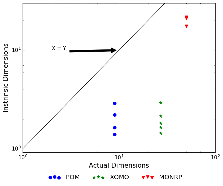
Figure 10: The (log of) actual dimensions are shown on the x-axis and (log of) intrinsic dimensionality is shown on the y-axis. The intrinsic dimensionality of the systems are much lower than the actual dimensionality (number of columns in the dataset) - this can be easily observed since all the points are lower the line $x=y$, which means points where actual dimensions is equal to intrinsic dimension.

9.2 Testing technique

Given our hypothesis that the problem space lies in a lower dimensional hyperplane — it is imperative to demonstrate that the intrinsic dimensionality of the configuration space is less than the actual dimension. To formalize this notion, we borrow the concept of correlation dimension from the domain of physics [24]. The correlation dimension of a dataset with $k$ items is found by computing the number of items found at distance within radius $r$ (where r is the Euclidean distance between two configurations) while varying $r$. This is then normalized by the number of connections between $k$ items to find the expected number of neighbors at distance $r$. This can be written as:

$$C(r)=\frac{2}{k(k-1)}\displaystyle\sum_{i=1}^{n}\displaystyle\sum_{j=i+1}^{n}I(||x_{i},x_{j}||<r)\\$$ (4)

$$where:I(x<y)=\begin{cases}1,\text{ if x \textless y}\\ 0,\text{ otherwise}\\ \end{cases}$$

Given the dataset with $k$ items and range of distances [$r_{0}$–$r_{max}$], we estimate the intrinsic dimensionality as the mean slope between $\ln(C(r))$ and $\ln(r)$.

9.3 Evaluation

On the space of problems explored in this paper, we observe that the intrinsic dimensionality of the problems is much lower than the actual dimension. Figure 10 presents the intrinsic dimensionality along with the actual dimensions of the software systems. If we look at the intrinsic dimensionality and compare it with the actual dimensionality, then it becomes apparent that the configuration space lies on a lower dimensional hyperplane. For example, the MONRP family of problems has 50-dimensional decision space, but the average intrinsic dimensionality of the space is just $20.39$ (this is a fractal dimension). At the heart of SWAY is WHERE (a spectral clusterer), which uses the approximation of the first principal component to divide the configuration space and hence can take advantage of the low intrinsic dimensionality.

As a summary, our observations indicate that the intrinsic dimension of the problem space explored in this paper is much lower than its actual dimension.

Hence, recursive top-down clustering based on the intrinsic dimensions rather than the actual dimension is be more effective. In other words, decision space with similar performance values lie closer to the intrinsic hyperplane, compared to the actual dimensions.

With this hypothesis, SWAY recursively cluster candidates basing on intrinsic dimensions only. Also, with the assumption genotype - phenotype space mapping assumption (see §4.1), SWAY does not need to evaluate every candidates, making SWAY so quickly to terminate.

10 Threats to Validity

10.1 Optimizer bias

There are theoretical reasons to conclude that it is impossible to show that any one optimizer always performs best. Wolpert and Macready [65] showed in 1997 that no optimizers necessarily work better than any other for all possible optimization problems.

In this study, we compared Sway framework with NSGA-II, SPEA2, GALE for XOMO, POM3 and MONRP case studies. We selected those learners since:

• The literature review of Sayyad et al. [54] reported that NSGA-II and SPEA2 were widely used in the SBSE literature;

• GALE is the successor of SWAY and this study was partly to show how sampling feature of GALE is the reason why GALE is competitive against widely used evolutionary algorithms.

That said, there exist many other optimizers. For examples, NSGA-III is an improved version of NSGA-II, which can get better diversity of the results. Such kind of optimizers might perform better than Sway method. Also, for some specific problem, researchers might propose some modified version of MOEAs. For such kind of modified/optimized algorithms, Sway might not perform as well as them.

10.2 Sampling bias

We used the XOMO, POM3 and MONRP SE problems for our case studies. We found that in all of these problems, SWAY can perform as well (or better) as other MOEAs. However, there are many other optimization problems in the area of SE.

It is very difficult to find the representatives sample of models which covers all kinds of models. Some problems might have other properties which make it different from any problem we tested in this study. For example, project planning problem is an open question up to now. In the project planning problem, there are constraints which organized as the directed acyclic graph(DAG). None of problems we tested with such kind of constraints.

For this issue of sampling bias (and for optimizer bias), we cannot explore all problems here. What we can do:

• Detail our current work and encourage other researchers to test our software on a wider range of problems;

• In future work, apply Sway when we come across a new problem and compare them to the existed algorithms.

10.3 Evaluation bias

We evaluated the results through spread and hypervolume and number of evaluations. There are many other measures which are adopted in the community of software engineering. For example, a widely used evaluation measures for the multi-objective optimization problem is the inverted generational distance (igd) indicator [61].

Using various measures might lead to different conclusions. This threatens our conclusion. A comprehensive analysis using other measures is left to the future work.

11 Future Work

We focused on three SBSE problems – two for software management (XOMO and POM), and another for requirement engineering (MONRP). In the future, we will explore problems in software testing– an important area in search based software engineering. Recently, Panichella et al. [49, 50] addressed that software testing should be extended into a multi-objective optimization, instead of just consideration the “branch coverage rate”, making such problems trickier.

Another area for future work is to explore sampling methods for single-objective problems. In this paper, we were focusing on multi-objective problems. For multi-objective problems, one essential target is the diversity of results; while in single-objective optimization problems, we hope to find out single best configurations. Perhaps in that simpler domain, methods like SWAY outperform existing state-of-the-art methods.

One assumption of SWAY is the genotype-phenotype mapping of the explored problem space (see §4.1). In the future, we could possibly improve SWAY via regressions between specific variables (instead of whole decision variables) and objectives.

Finally, in this paper, SWAY selects from a large pool of candidates generated initially. An alternate strategy that might be useful would be to build sample candidates adaptive (e.g. using Bayesian parameter optimization or Estimation of Distribution Algorithms [36]). Such an approach might help avoid unnecessary candidate generation.

12 Conclusion

In this paper we introduce an alternative to evolutionary algorithms for solving SBSE problems. The major drawback of EAs is the slow convergence of solutions, which means it requires too many evaluations/measurements to solve a problem. To overcome this limitation we introduce SWAY, which explores the concept of sampling. The key idea of SWAY is to use the underlying dimension of the problem to recursively sample the solutions, while only evaluating the extreme points in the decision space. This strategy helps us to reduce the number of evaluations to find “interesting” solutions.

We evaluated SWAY on three SE models, which includes models with continuous as well as discrete space. Our approach achieves similar performance (hypervolume and spread), if not better, when compared to other sophisticated optimizers using far fewer evaluations ($\frac{1}{20}$ of evaluations used by traditional EAs).

We demonstrate how SWAY can be adapted to suit various problems. As an example, we show how barebone SWAY, which is applicable for problems on the continuous domains, can be adapted for constrained problem in discrete space. Furthermore, we explore the possibility of using the results from SWAY to “super-charge” traditional EAs. We find that supercharging traditional EAs with solutions from SWAY does not improve their performance significantly.

Hence, our observations lead us to believe that sampling is a cheaper alternative to the more expensive and sophisticated evolutionary techniques. We also believe that techniques such as SWAY, which exploit the underlying dimension of the problem space, would be very useful to solve problems, where the practitioners are not at the liberty to perform thousands of evaluations. Observation is in line with a current trend in machine learning research. Dasgupta and Freund [14] comment that:

A recent positive in that field has been the realization that a lot of data which superficially lie in a very high-dimensional space $R^{D}$, actually have low intrinsic dimension, in the sense of lying close to a manifold of dimension $d\ll D$.

With this paper we want to propagate the message of “easy over hard” and we believe SWAY is a step towards this direction. Even in domains where SWAY does not outperform other evolutionary algorithms, we would still suggest researchers to first apply SWAY, since this is a simple and fast algorithm which can rapidly produce baseline results.

References

- [1] A. Arcuri and L. Briand. A practical guide for using statistical tests to assess randomized algorithms in software engineering. In ICSE’11, pages 1–10, 2011.
- [2] Ery Arias-Castro, Gilad Lerman, and Teng Zhang. Spectral clustering based on local pca. Journal of Machine Learning Research, 18(9):1–57, 2017.
- [3] Johannes Bader and Eckart Zitzler. Hype: An algorithm for fast hypervolume-based many-objective optimization. Evolutionary computation, 19(1):45–76, 2011.
- [4] Anthony J. Bagnall, Victor J. Rayward-Smith, and Ian M Whittley. The next release problem. Information and software technology, 43(14):883–890, 2001.
- [5] Aurélien Bellet and Pascal Denis. Spectral graph-based methods for learning word embeddings. 2016.
- [6] Nicolas Bettenburg, Meiyappan Nagappan, and Ahmed E Hassan. Think locally, act globally: Improving defect and effort prediction models. In Proceedings of the 9th IEEE Working Conference on Mining Software Repositories, pages 60–69. IEEE Press, 2012.
- [7] Nicolas Bettenburg, Meiyappan Nagappan, and Ahmed E Hassan. Towards improving statistical modeling of software engineering data: think locally, act globally! Empirical Software Engineering, 20(2):294–335, 2015.
- [8] Ella Bingham and Heikki Mannila. Random projection in dimensionality reduction: applications to image and text data. In Proceedings of the seventh ACM SIGKDD international conference on Knowledge discovery and data mining, pages 245–250. ACM, 2001.
- [9] B. Boehm and R. Turner. Using risk to balance agile and plan-driven methods. Computer, 2003.
- [10] Barry Boehm, Ellis Horowitz, Ray Madachy, Donald Reifer, Bradford K. Clark, Bert Steece, A. Winsor Brown, Sunita Chulani, and Chris Abts. Software Cost Estimation with Cocomo II. Prentice Hall, 2000.
- [11] Barry Boehm and Richard Turner. Balancing Agility and Discipline: A Guide for the Perplexed. Addison-Wesley Longman Publishing Co., Inc., 2003.
- [12] Richard E. Brown, Eric R. Masanet, Bruce Nordman, William F. Tschudi, Arman Shehabi, John Stanley, Jonathan G. Koomey, Dale A. Sartor, and Peter T. Chan. Report to congress on server and data center energy efficiency: Public law 109-431. 06/2008 2008.
- [13] Coral Calero and Mario Piattini. Green in software engineering, 2015.
- [14] Sanjoy Dasgupta and Yoav Freund. Random projection trees and low dimensional manifolds. In 40th ACM Symposium on Theory of Computing, 2008.
- [15] Kalyanmoy Deb, Amrit Pratap, Sameer Agarwal, and T. Meyarivan. A fast elitist multi-objective genetic algorithm: NSGA-II. IEEE Transactions on Evolutionary Computation, 2000.
- [16] Kalyanmoy Deb, Lothar Thiele, Marco Laumanns, and Eckart Zitzler. Scalable Test Problems for Evolutionary Multi-Objective Optimization. TIK Report 1990, Computer Engineering and Networks Laboratory (TIK), ETH Zurich, July 2001.
- [17] Constanze Deiters, Andreas Rausch, and Marco Schindler. Using spectral clustering to automate identification and optimization of component structures. In Realizing Artificial Intelligence Synergies in Software Engineering (RAISE), 2013 2nd International Workshop on, pages 14–20. IEEE, 2013.
- [18] Juan J Durillo, Yuanyuan Zhang, Enrique Alba, Mark Harman, and Antonio J Nebro. A study of the bi-objective next release problem. Empirical Software Engineering, 16(1):29–60, 2011.
- [19] Juan J Durillo, YuanYuan Zhang, Enrique Alba, and Antonio J Nebro. A study of the multi-objective next release problem. In Proceedings of the 1st International Symposium on Search Based Software Engineering (SSBSE’09), pages 49–58, 2009.
- [20] Bradley Efron and Robert J Tibshirani. An introduction to the bootstrap. CRC, 1993.
- [21] Christos Faloutsos and King-Ip Lin. FastMap: A fast algorithm for indexing, data-mining and visualization of traditional and multimedia datasets, volume 24. ACM, 1995.
- [22] Danyel Fisher, Rob DeLine, Mary Czerwinski, and Steven Drucker. Interactions with big data analytics. interactions, 19(3):50–59, May 2012.
- [23] B. Ghotra, S. McIntosh, and A. E. Hassan. Revisiting the impact of classification techniques on the performance of defect prediction models. In 37th IEEE International Conference on Software Engineering, May 2015.
- [24] Peter Grassberger and Itamar Procaccia. Measuring the strangeness of strange attractors. In The Theory of Chaotic Attractors, pages 170–189. Springer, 2004.
- [25] Mark Harman, S. Afshin Mansouri, and Yuanyuan Zhang. Search-based software engineering: Trends, techniques and applications. ACM Comput. Surv., 45(1):11:1–11:61, December 2012.
- [26] Andrzej Jaszkiewicz. On the performance of multiple-objective genetic local search on the 0/1 knapsack problem-a comparative experiment. IEEE Transactions on Evolutionary Computation, 6(4):402–412, 2002.
- [27] Ian Jolliffe. Principal component analysis. Wiley Online Library, 2002.
- [28] Sepandar D. Kamvar, Dan Klein, and Christopher D. Manning. Spectral learning. In Proceedings of the 18th International Joint Conference on Artificial Intelligence, IJCAI’03, pages 561–566, San Francisco, CA, USA, 2003. Morgan Kaufmann Publishers Inc.
- [29] Joshua Knowles and David Corne. The pareto archived evolution strategy: A new baseline algorithm for pareto multiobjective optimisation. In Evolutionary Computation, 1999. CEC 99. Proceedings of the 1999 Congress on, volume 1. IEEE, 1999.
- [30] J. Krall, T. Menzies, and M. Davies. Geometric active learning for software engineering. Under-Review, IEEE TSE, 2014.
- [31] Joseph Krall. Faster Evolutionary Multi-Objective Optimization via GALE, the Geometric Active Learner. PhD thesis, West Virginia University, 2014. http://goo.gl/u8ganF.
- [32] Joseph Krall, Tim Menzies, and Misty Davies. Learning the task management space of an aircraft approach model. In Proceedings of the 2014 AAAI Conference, AAAI’14, 2014.
- [33] Joseph Krall, Tim Menzies, and Misty Davies. Better model-based analysis of human factors for safe aircraft approach. IEEE Transactions on Human-Machine Systems, 2015.
- [34] Joseph Krall, Tim Menzies, and Misty Davies. Gale: Geometric active learning for search-based software engineering. IEEE Transactions on Software Engineering, 2015.
- [35] Rakesh Kumar, Keith I. Farkas, Norman P. Jouppi, Parthasarathy Ranganathan, and Dean M. Tullsen. Single-isa heterogeneous multi-core architectures: The potential for processor power reduction. In Proceedings of the 36th Annual IEEE/ACM International Symposium on Microarchitecture, MICRO 36, pages 81–, 2003.
- [36] Pedro Larranaga. A review on estimation of distribution algorithms. In Estimation of distribution algorithms, pages 57–100. Springer, 2002.
- [37] Naveen Kumar Lekkalapudi. Cross trees: Visualizing estimations using decision trees. West Virginia University, 2014.
- [38] Huamin Li, Yuval Kluger, and Mark Tygert. Randomized algorithms for distributed computation of principal component analysis and singular value decomposition. arXiv preprint arXiv:1612.08709, 2016.
- [39] Francisco Luna, David L González-Álvarez, Francisco Chicano, and Miguel A Vega-Rodríguez. The software project scheduling problem: A scalability analysis of multi-objective metaheuristics. Applied Soft Computing, 15:136–148, 2014.
- [40] Makoto Matsumoto and Takuji Nishimura. Mersenne twister: a 623-dimensionally equidistributed uniform pseudo-random number generator. ACM Transactions on Modeling and Computer Simulation (TOMACS), 8(1):3–30, 1998.
- [41] Tim Menzies, Oussama El-Rawas, J. Hihn, M. Feather, R. Madachy, and B. Boehm. The business case for automated software engineerng. In 22nd IEEE/ACM International Conference on Automated Software Engineering, 2007.
- [42] Tim Menzies and Ying Hu. Data mining for very busy people. Computer, 36(11):22–29, 2003.
- [43] Tim Menzies, David Owen, and Julian Richardson. The strangest thing about software. Computer, 40(1), 2007.
- [44] Tim Menzies, S. Williams, Oussama El-Rawas, D. Baker, B. Boehm, J. Hihn, K. Lum, and R. Madachy. Accurate estimates without local data? Software Process Improvement and Practice, 2009.
- [45] Tim Menzies, S. Williams, Oussama El-Rawas, B. Boehm, and J. Hihn. How to avoid drastic software process change (using stochastic stability). In 31st International Conference on Software Engineering, 2009.
- [46] Nikolaos Mittas and Lefteris Angelis. Ranking and Clustering Software Cost Estimation Models through a Multiple Comparisons Algorithm. IEEE Transactions of Software Engineering, 2013.
- [47] G. E. Moore. Cramming more components onto integrated circuits. Proceedings of the IEEE, 86(1):82–85, Jan 1998.
- [48] Vivek Nair, Tim Menzies, and Jianfeng Chen. An (accidental) exploration of alternatives to evolutionary algorithms for sbse. In International Symposium on Search Based Software Engineering, pages 96–111. Springer, 2016.
- [49] Annibale Panichella, Fitsum Kifetew, and Paolo Tonella. Automated test case generation as a many-objective optimisation problem with dynamic selection of the targets. IEEE Transactions on Software Engineering, 2017.
- [50] Annibale Panichella, Fitsum Meshesha Kifetew, and Paolo Tonella. Reformulating branch coverage as a many-objective optimization problem. In Software Testing, Verification and Validation (ICST), 2015 IEEE 8th International Conference on, pages 1–10. IEEE, 2015.
- [51] D. Port, A. Olkov, and T. Menzies. Using simulation to investigate requirements prioritization strategies. In 23rd International Conference on Automated Software Engineering, 2008.
- [52] Shelley Redgate, Wendy Tindale, John Fenner, Abdallah Al-Mohammad, and David Barber. Principal component analysis as a method of respiratory motion detection on a solid state czt dedicated cardiac camera. Journal of Nuclear Medicine, 57(supplement 2):1969–1969, 2016.
- [53] Patrick Reed, Joshua B Kollat, and VK Devireddy. Using interactive archives in evolutionary multiobjective optimization: A case study for long-term groundwater monitoring design. Environmental Modelling & Software, 2007.
- [54] A. Sayyad, J. Ingram, T. Menzies, and H. Ammar. Scalable product line configuration: A straw to break the camel’s back. In 28th International Conference on Automated Software Engineering, 2013.
- [55] Abdel Sayyad and Hany Ammar. Pareto-optimal search-based software engineering (POSBSE): A literature survey. In 2nd International Workshop on Realizing Artificial Intelligence Synergies in Software Engineering, 2013.
- [56] Jian-Feng Shi, Steve Ulrich, and Stephane Ruel. Spacecraft pose estimation using principal component analysis and a monocular camera. In AIAA Guidance, Navigation, and Control Conference, page 1034, 2017.
- [57] Jianbo Shi and Jitendra Malik. Normalized cuts and image segmentation. Pattern Analysis and Machine Intelligence, IEEE Transactions on, 22(8):888–905, 2000.
- [58] Stanley Smith Stevens. On the theory of scales of measurement. 1946.
- [59] Chakkrit Tantithamthavorn, Shane McIntosh, Ahmed E Hassan, and Kenichi Matsumoto. Automated parameter optimization of classification techniques for defect prediction models. In 38th International Conference on Software Engineering, 2016.
- [60] Patrick Thibodeau. Data centers are the new polluters, august 26, 2014. Available from http://v.gd/TpSdZn.
- [61] David A Van Veldhuizen and Gary B Lamont. Multiobjective evolutionary algorithm research: A history and analysis. Technical report, Citeseer, 1998.
- [62] András Vargha and Harold D Delaney. A Critique and Improvement of the CL Common Language Effect Size Statistics of McGraw and Wong. Journal of Educational and Behavioral Statistics, 2000.
- [63] Tiantian Wang, Mark Harman, Yue Jia, and Jens Krinke. Searching for better configurations: A rigorous approach to clone evaluation. In 9th Joint Meeting on Foundations of Software Engineering. ACM, 2013.
- [64] Tiantian Wang, Mark Harman, Yue Jia, and Jens Krinke. Searching for better configurations: a rigorous approach to clone evaluation. In Proceedings of the 2013 9th Joint Meeting on Foundations of Software Engineering, pages 455–465. ACM, 2013.
- [65] D.H. Wolpert and W.G. Macready. No free lunch theorems for optimization. Evolutionary Computation, IEEE Transactions on, 1(1):67–82, Apr 1997.
- [66] Feng Zhang, Quan Zheng, Ying Zou, and Ahmed E. Hassan. Cross-project defect prediction using a connectivity-based unsupervised classifier. In Proceedings of the 38th International Conference on Software Engineering (ICSE’16), 2016.
- [67] Qingfu Zhang and Hui Li. Moea/d: A multiobjective evolutionary algorithm based on decomposition. IEEE Transactions on evolutionary computation, 11(6):712–731, 2007.
- [68] Eckart Zitzler and Simon Künzli. Indicator-based selection in multiobjective search. In 8th International Conference on Parallel Problem Solving from Nature. Springer, 2004.
- [69] Eckart Zitzler and Simon Künzli. Indicator-based selection in multiobjective search. In International Conference on Parallel Problem Solving from Nature, pages 832–842. Springer, 2004.
- [70] Eckart Zitzler, Marco Laumanns, and Lothar Thiele. SPEA2: Improving the strength pareto evolutionary algorithm. Technical report, 2001.
- [71] Eckart Zitzler, Marco Laumanns, and Lothar Thiele. SPEA2: Improving the strength pareto evolutionary algorithm for multiobjective optimization. In Evolutionary Methods for Design, Optimisation, and Control. CIMNE, 2002.
- [72] Eckart Zitzler and Lothar Thiele. Multiobjective optimization using evolutionary algorithms - a comparative case study. In Parallel problem solving from nature. Springer, 1998.
- [73] Marcela Zuluaga, Andreas Krause, Guillaume Sergent, and Markus Püschel. Active learning for multi-objective optimization. In International Conference on Machine Learning (ICML), 2013.