On discrete structures in finite Hilbert spaces

Abstract

We present a brief review of discrete structures in a finite Hilbert space, relevant for the theory of quantum information. Unitary operator bases, mutually unbiased bases, Clifford group and stabilizer states, discrete Wigner function, symmetric informationally complete measurements, projective and unitary t–designs are discussed. Some recent results in the field are covered and several important open questions are formulated. We advocate a geometric approach to the subject and emphasize numerous links to various mathematical problems

e-mail: ingemar@physto.se  karol@cft.edu.pl

I Introduction

These notes are based on a new chapter written to the second edition of our book Geometry of Quantum States. An introduction to Quantum Entanglement BZ06 . The book is written at the graduate level for a reader familiar with the principles of quantum mechanics. It is targeted first of all for readers who do not read the mathematical literature everyday, but we hope that students of mathematics and of the information sciences will find it useful as well, since they also may wish to learn about quantum entanglement.

Individual chapters of the book are to a large extent independent of each other. For instance, we hope that the new chapter presented here might become a source of information on recent developments on discrete structures in finite Hilbert space also for experts working in the field. Therefore we have compiled these notes, which aim to present an introduction to the subject as well as an up to date review on basic features of objects belonging to the Hilbert space and important for the field of quantum information processing.

Quantum state spaces are continuous, but they have some intriguing realizations of discrete structures hidden inside. We will discuss some of them, starting from unitary operator bases, a notion of strategic importance in the theory of entanglement, signal processing, quantum computation, and more. The structures we are aiming at are known under strange acronyms such as ‘MUB’ and ‘SIC’. They will be spelled out in due course, but in most of the chapter we let the Heisenberg groups occupy the centre stage. It seems that the Heisenberg groups understand what is going on.

All references to equations or the numbers of section refers to the draft of the second edition of the book. To give a reader a better orientation on the topics covered we provide its contents in Appendix A. The second edition of the book includes also a new chapter 17 on multipartite entanglement BZ16 and several other new sections.

II Unitary operator bases and the Heisenberg groups

Starting from a Hilbert space ${\cal H}$ of dimension $N$ we have another Hilbert space of dimension $N^{2}$ for free, namely the Hilbert-Schmidt space of all complex operators acting on ${\cal H}$, canonically isomorphic to the Hilbert space ${\cal H}\otimes{\cal H}^{*}$. It was introduced in Section 8.1 and further explored in Chapter 9. Is it possible to find an orthonormal basis in ${\cal H}\otimes{\cal H}^{*}$ consisting solely of unitary operators? A priori this looks doubtful, since the set of unitary matrices has real dimension $N^{2}$, only one half the real dimension of ${\cal H}\otimes{\cal H}^{*}$. But physical observables are naturally associated to unitary operators, so if such bases exist they are likely to be important. They are called unitary operator bases, were introduced by Schwinger (1960) Schw60 , and heavily used by him Schw03 .

In fact unitary operator bases do exist, in great abundance. And we can ask for more Kni96 . We can insist that the elements of the basis form a group. More precisely, let $\bar{G}$ be a finite group of order $N^{2}$, with identity element $e$. Let $U_{g}$ be unitary operators giving a projective representation of $\bar{G}$, such that

1. $U_{e}$ is the identity matrix.

2. $g\neq e$     $\Rightarrow$     Tr$U_{g}=0$.

3. $U_{g}U_{h}=\lambda(g,h)U_{gh}$, where $|\lambda(g,h)|=1$.

(So $\lambda$ is a phase factor.) Then this collection of unitary matrices is a unitary operator basis. To see this, observe that

$$U_{g}^{\dagger}=\lambda(g^{-1},g)^{-1}U_{g^{-1}}\ .$$ (1)

It follows that

$$g^{-1}h\neq e\hskip 14.22636pt\Rightarrow\hskip 14.22636pt\mbox{Tr}U_{g}^{\dagger}U_{h}=0\ ,$$ (2)

and moreover that Tr$U_{g}^{\dagger}U_{g}=\mbox{Tr}U_{e}=N$. Hence these matrices are orthogonal with respect to the Hilbert-Schmidt inner product from Section 8.1. Unitary operator bases arising from a group in this way are known as unitary operator bases of group type, or as nice error bases—a name that comes from the theory of quantum computation (where they are used to discretize errors, thus making the latter correctable—as we will see in Section 17.7).

The question of the existence of nice error bases is a question in group theory. First of all we note that there are two groups involved in the construction, the group $G$ which is faithfully represented by the above formulas, and the collineation group $\bar{G}$ which is the group $G$ with all phase factors ignored. The group $\bar{G}$ is also known, in this context, as the index group. Unless $N$ is a prime number (in which case the nice error bases are essentially unique), there is a long list of possible index groups. An abelian index group is necessarily of the form $H\times H$, where $H$ is an abelian group. Non-abelian index groups are more difficult to classify, but it is known that every index group must be soluble. The classification problem has been studied by Klappenecker and Rötteler Kla02 , making use of the classification of finite groups. They also maintain an on-line catalogue. Soluble groups will reappear in Section IX; for the moment let us just mention that all abelian groups are soluble.

The paradigmatic example of a group $G$ giving rise to a unitary operator basis is the Weyl–Heisenberg group $H(N)$. This group appeared in many different contexts, starting in nineteenth century algebraic geometry, and in the beginnings of matrix theory Syl82 . In the twentieth century it took on a major role in the theory of elliptic curves Mum83 . Weyl (1932) Wey32 studied its unitary representations in his book on quantum mechanics. The group $H(N)$ can be presented as follows. Introduce three group elements $X$, $Z$, and $\omega$. Declare them to be of order $N$:

$$X^{N}=Z^{N}=\omega^{N}={\mathbbm{1}}\ .$$ (3)

Insist that $\omega$ belongs to the centre of the group (it commutes with everything):

$$\omega X=X\omega\ ,\hskip 22.76219pt\omega Z=Z\omega\ ,$$ (4)

Then we impose one further key relation:

$$ZXZ^{-1}X^{-1}=\omega\hskip 14.22636pt\Leftrightarrow\hskip 14.22636ptZX=\omega XZ\ .$$ (5)

The Weyl–Heisenberg group consists of all ‘words’ that can be written down using the three ‘letters’ $\omega$, $X$, $Z$, subject to the above relations. It requires no great effort to see that it suffices to consider $N^{3}$ words of the form $\omega^{t}X^{r}Z^{s}$, where $t,r,s$ are integers modulo $N$.

The Weyl–Heisenberg group admits an essentially unique unitary representation in dimension $N$. First we represent $\omega$ as multiplication with a phase factor which is a primitive root of unity, conveniently chosen to be

$$\omega=e^{2\pi i/N}\ .$$ (6)

If we further insist that $Z$ be represented by a diagonal operator we are led to the clock-and-shift representation

$$Z|i\rangle=\omega^{i}|i\rangle\ ,\hskip 17.07164ptX|i\rangle=|i+1\rangle\ .$$ (7)

The basis kets are labelled by integers modulo $N$. A very important area of application for the Weyl–Heisenberg group is that of time-frequency analysis of signals; then the operators $X$ and $Z$ may represent time delays and Doppler shifts of a returning radar wave form. But here we stick to the language of quantum mechanics and refer to Howard et al. HCM06 for an introduction to signal processing and radar applications.

To orient ourselves we first write down the matrix form of the generators for $N=3$, which is a good choice for illustrative purposes:

$$Z=\left(\begin{array}[]{ccc}1&0&0\\ 0&\omega&0\\ 0&0&\omega^{2}\end{array}\right)\ ,\hskip 17.07164ptX=\left(\begin{array}[]{ccc}0&0&1\\ 1&0&0\\ 0&1&0\end{array}\right)\ .$$ (8)

In two dimensions $Z$ and $X$ become the Pauli matrices $\sigma_{z}$ and $\sigma_{x}$ respectively. We note the resemblance between eq. (5) and a special case of the equation that defines the original Heisenberg group, eq. (6.4). This explains why Weyl took this finite group as a toy model of the latter. We also note that although the Weyl–Heisenberg group has order $N^{3}$ its collineation group—the group modulo phase factors, which is the group acting on projective space—has order $N^{2}$. In fact the collineation group is an abelian product of two cyclic groups, $Z_{N}\times Z_{N}$. The slight departure from commutativity ensures an interesting representation theory.

There is a complication to notice at this point: because $\det{Z}=\det{X}=(-1)^{N+1}$, it matters if $N$ is odd or even. If $N$ is odd the Weyl–Heisenberg group is a subgroup of $SU(N)$, but if $N$ is even it is a subgroup of $U(N)$ only. Moreover, if $N$ is odd the $N$th power of every group element is the identity, but if $N$ is even we must go to the $2N$th power to say as much. (For $N=2$ we find $X^{2}=Z^{2}={\mathbbm{1}}$ but $(ZX)^{2}=(i\sigma_{y})^{2}=-{\mathbbm{1}}$.) These annoying facts make even dimensions significantly more difficult to handle, and leads to the definition

$$\bar{N}=\left\{\begin{array}[]{lll}N&\mbox{if}&N\ \mbox{is odd}\\ 2N&\mbox{if}&N\ \mbox{is even.}\end{array}\right.$$ (9)

Keeping the complication in mind we turn to the problem of choosing suitable phase factors for the $N^{2}$ words that will make up our nice error basis. The peculiarities of even dimensions suggest an odd-looking move. We introduce the phase factor

$$\tau\equiv-e^{\pi i/N}=-\sqrt{\omega}\ ,\hskip 22.76219pt\tau^{\bar{N}}=1\ .$$ (10)

Note that $\tau$ is an $N$th root of unity only if $N$ is odd. Then we define the displacement operators

$$D_{\bf p}\equiv D_{r,s}=\tau^{rs}X^{r}Z^{s}\ ,\hskip 22.76219pt0\leq r,s\leq\bar{N}-1\ .$$ (11)

These are the words to use in the error basis. The double notation—using either $D_{\bf p}$ or $D_{r,s}$—emphasizes that it is convenient to view $r,s$ as the two components of a ‘vector’ ${\bf p}$. Because of the phase factor $\tau$ the displacement operators are not actually in the Weyl–Heisenberg group, as originally defined, if $N$ is even. So there is a price to pay for this, but in return we get the group law in the form

$$D_{r,s}D_{u,v}=\omega^{us-vr}D_{u,v}D_{r,s}=\tau^{us-vr}D_{r+u,s+v}$$

$$\Leftrightarrow$$ (12)

$$D_{\bf p}D_{\bf q}=\omega^{\Omega({\bf p},{\bf q})}D_{\bf q}D_{\bf p}=\tau^{\Omega({\bf p},{\bf q})}D_{{\bf p}+{\bf q}}\ .$$

The expression in the exponent of the phase factors is anti-symmetric in the ‘vectors’ that label the displacement operators. In fact $\Omega({\bf p},{\bf q})$ is a symplectic form (see Section 3.4), and a very nice object to encounter.

A desirable by-product of our conventions is

$$D^{-1}_{r,s}=D_{r,s}^{\dagger}=D_{-r,-s}\ .$$ (13)

Another nice feature is that the phase factor ensures that all displacement operators are of order $N$. On the other hand we have $D_{r+N,s}=\tau^{Ns}D_{r,s}$. This means that we have to live with a treacherous sign if $N$ is even, since the displacement operators are indexed by integers modulo $2N$ in that case. Even dimensions are unavoidably difficult to deal with. (We do not know who first commented that “even dimensions are odd”, but he or she had a point.)

Finally, and importantly, we observe that

$$\mbox{Tr}D_{r,s}=\tau^{rs}\sum_{i=0}^{N-1}\omega^{si}\langle i|i+r\rangle=N\delta_{r,0}\delta_{s,0}\ .$$ (14)

Thus all the displacement operators except the identity are represented by traceless matrices, which means that the Weyl–Heisenberg group does indeed provide a unitary operator basis of group type, a nice error basis. Any complex operator $A$ on ${\cal H}_{N}$ can be written, uniquely, in the form

$$A=\sum_{r=0}^{N-1}\sum_{s=0}^{N-1}a_{rs}D_{r,s}\ ,$$ (15)

where the expansion coefficients $a_{rs}$ are complex numbers given by

$$a_{rs}=\frac{1}{N}\mbox{Tr}D_{r,s}^{\dagger}A=\frac{1}{N}\mbox{Tr}D_{-r,-s}A\ .$$ (16)

Again we are using the Hilbert-Schmidt scalar product from Section 8.1. Such expansions were called ‘quantum Fourier transformations’ in Section 6.2.

III Prime, composite, and prime power dimensions

The Weyl–Heisenberg group cares deeply whether the dimension $N$ is given by a prime number (denoted $p$), or by a composite number (say $N=p_{1}p_{2}$ or $N=p^{K}$). If $N=p$ then every element in the group has order $N$ (or $\bar{N}$ if $N=2$), except of course for the identity element. If on the other hand $N=p_{1}p_{2}$ then $(Z^{p_{1}})^{p_{2}}={\mathbbm{1}}$, meaning that the element $Z^{p_{1}}$ has order $p_{2}$ only. This is a striking difference between prime and composite dimensions.

The point is that we are performing arithmetic modulo $N$, which means that we regard all integers that differ by multiples of $N$ as identical. With this understanding, we can add, subtract, and multiply the integers freely. We say that integers modulo $N$ form a ring, just as the ordinary integers do. If $N$ is composite it can happen that $xy=0$ modulo $N$, even though the integers $x$ and $y$ are non-zero. For instance, $2\cdot 2=0$ modulo 4. As Problem 12.2 should make clear, a ring is all we need to define a Heisenberg group, so we can proceed anyway. However, things work more smoothly if $N$ equals a prime number $p$, because of the striking fact that every non-zero integer has a multiplicative inverse modulo $p$. Integers modulo $p$ form a field, which by definition is a ring whose non-zero members form an abelian group under multiplication, so that we can perform division as well. In a field—the set of rational numbers is a standard example—we can perform addition, subtraction, multiplication, and division. In a ring—such as the set of all the integers—division sometimes fails. The distinction becomes important in Hilbert space once the latter is being organized by the Weyl–Heisenberg group.

The field of integers modulo a prime $p$ is denoted ${\mathbb{Z}}_{p}$. When the dimension $N=p$ the operators $D_{\bf p}$ can be regarded as indexed by elements ${\bf p}$ of a two dimensional vector space. (We use the same notation for arbitrary $N$, but in general we need quotation marks around the word ‘vector’. In a true vector space the scalar numbers must belong to a field.) Note that this vector space contains $p^{2}$ vectors only. Now, whenever we encountered a vector space in this book, we tended to focus on the set of lines through its origin. This is a fruitful thing to do here as well. Each such line consists of all vectors ${\bf p}$ obeying the equation ${\bf a}\cdot{\bf p}=0$ for some fixed vector ${\bf a}$. Since ${\bf a}$ is determined only up to an overall factor we obtain $p+1$ lines in all, given by

$${\bf a}=\left(\begin{array}[]{c}a_{1}\\ a_{2}\end{array}\right)\in\left\{\left(\begin{array}[]{c}0\\ 1\end{array}\right),\ \left(\begin{array}[]{c}1\\ 0\end{array}\right),\ \left(\begin{array}[]{c}1\\ 1\end{array}\right),\ \dots\ ,\ \left(\begin{array}[]{c}1\\ p-1\end{array}\right)\right\}\ .$$ (17)

This set of lines through the origin is a projective space with only $p+1$ points. Of more immediate interest is the fact that these lines through the origin correspond to cyclic subgroups of the Weyl–Heisenberg group, and indeed to its maximal abelian subgroups. (Choosing ${\bf a}=(1,x)$ gives the cyclic subgroup generated by $D_{-x,1}$.) The joint eigenbases of such subgroups are related in an interesting way, which will be the subject of Section V.

Readers who want a simple story are advised to ignore everything we say about non-prime dimensions. With this warning, we ask: What happens when the dimension is not prime? On the physical side this is often the case: we may build a Hilbert space of high dimension by taking the tensor product of a large number of Hilbert spaces which individually have a small dimension (perhaps to have a Hilbert space suitable for describing many atoms). This immediately suggests that it might be interesting to study the direct product $H(N_{1})\times H(N_{2})$ of two Weyl–Heisenberg groups, acting on the tensor product space ${\cal H}_{N_{1}}\otimes{\cal H}_{N_{2}}$. (Irreducible representations of a direct product of groups always act on the tensor product of their representation spaces.) Does this give something new?

On the group theoretical side it is known that the cyclic groups $Z_{N_{1}N_{2}}$ and $Z_{N_{1}}\times Z_{N_{2}}$ are isomorphic if and only if the integers ${N_{1}}$ and ${N_{2}}$ are relatively prime, that is to say if they do not contain any common factor. To see why, look at the examples $N=2\cdot 2$ and $N=2\cdot 3$. Clearly $Z_{2}\times Z_{2}$ contains only elements of order 2, hence it cannot be isomorphic to $Z_{4}$. On the other hand it is easy to verify that $Z_{2}\times Z_{3}=Z_{6}$. This observation carries over to the Weyl–Heisenberg group: the groups $H(N_{1}N_{2})$ and $H(N_{1})\times H(N_{2})$ are isomorphic if and only if $N_{1}$ and $N_{2}$ are relatively prime. Thus, in many composite dimensions including the physically interesting case $N=p^{K}$ we have a choice of more than one Heisenberg group to play with. They all form nice error bases. In applications to signal processing one sticks to $H(N)$ also when $N$ is large and composite, but in many-body physics and in the theory of quantum computation—carried out on tensor products of $K$ qubits, say—it is the multipartite Heisenberg group $H(p)^{\otimes K}=H(p)\times H(p)\times\dots\times H(p)$ that comes to the fore.

There is a way of looking at the group $H(p)^{\otimes K}$ which is quite analogous to our way of looking at $H(p)$. It employs finite fields with $p^{K}$ elements, and de-emphasizes the tensor product structure of the representation space—which in some situations is a disadvantage, but it is worth explaining anyway, especially since we will be touching on the theory of fields in Section IX. We begin by recalling how the field of complex numbers is constructed. One starts from the real field ${\mathbbm{R}}$, now called the ground field, and observes that the polynomial equation $P(x)\equiv x^{2}+1=0$ does not have a real solution. To remedy this the number ${\rm i}$ is introduced as a root of the equation $P(x)=0$. With this new number in hand the complex number field ${\mathbbm{C}}$ is constructed as a two-dimensional vector space over ${\mathbbm{R}}$, with $1$ and ${\rm i}$ as basis vectors. To multiply two complex numbers together we calculate modulo the polynomial $P(x)$, which simply amounts to setting ${\rm i}^{2}$ equal to $-1$ whenever it occurs. The finite fields $GF(p^{K})$ are defined in a similar way using the finite field ${\mathbbm{Z}}_{p}$ as a ground field. (Here ‘G’ stands for Galois. For a lively introduction to finite fields we refer to Arnold Arn11 . For quantum mechanical applications we recommend the review by Vourdas Vou04 ).

For an example, we may choose $p=2$. The polynomial $P(x)=x^{2}+x+1$ has no zeros in the ground field ${\mathbbm{Z}}_{2}$, so we introduce an ‘imaginary’ number $\alpha$ which is declared to obey $P(\alpha)=0$. Adding and multiplying in all possible ways, and noting that $\alpha^{2}=\alpha+1$ (using binary arithmetic), we obtain a larger field having $2^{2}$ elements of the form $x_{1}+x_{2}\alpha$, where $x_{1}$ and $x_{2}$ are integers modulo 2. This is the finite field $GF(p^{2})$. Interestingly its three non-zero elements can also be described as $\alpha$, $\alpha^{2}=\alpha+1$, and $\alpha^{3}=1$. The first representation is convenient for addition, the second for multiplication. We have a third description as the set of binary sequences $\{00,01,10,11\}$, and consequently a way of adding and multiplying binary sequences together. This is very useful in the theory of error-correcting codes Pl82 . But this is by the way.

By pursuing this idea it has been proven that there exists a finite field $GF(N)$ with $N$ elements if and only if $N=p^{K}$ is a power of prime number $p$, and moreover that this finite field is unique for a given $N$ (which is by no means obvious because there will typically exist several polynomials of the same degree having no solution modulo $p$). These fields can be regarded as $K$ dimensional vector spaces over the ground field ${\mathbbm{Z}}_{p}$, which is useful when we do addition. When we do multiplication it is helpful to observe the (non-obvious) fact that finite fields always contain a primitive element in terms of which every non-zero element of the field can be written as the primitive element raised to some integer power, so the non-zero elements form a cyclic group. Some further salient facts are:

• Every element obeys $x^{p^{K}}=x$.

• Every non-zero element obeys $x^{p^{K}-1}=1$.

• $GF(p^{K_{1}})$ is a subfield of $GF(p^{K_{2}})$ if and only if $K_{1}$ divides $K_{2}$.

The field with $2^{3}$ elements is presented in Table 1, and the field with $3^{2}$ elements is given as Problem 12.4.

Table 1: The field with 8 elements has irreducible polynomials $P_{1}(x)=x^{3}+x+1$ and $P_{2}(x)=x^{3}+x^{2}+1$; $\alpha$ is a root of $P_{1}(x)$.

Element	Polynomial	tr$x$	tr$x^{2}$	order
0 = 0	$x$	0	0	—
$\alpha^{7}=1$	$x+1$	1	1	1
$\alpha=\alpha$	$P_{1}(x)$	0	0	7
$\alpha^{2}=\alpha^{2}$	$P_{1}(x)$	0	0	7
$\alpha^{3}=\alpha+1$	$P_{2}(x)$	1	1	7
$\alpha^{4}=\alpha^{2}+\alpha$	$P_{1}(x)$	0	0	7
$\alpha^{5}=\alpha^{2}+\alpha+1$	$P_{2}(x)$	1	1	7
$\alpha^{6}=\alpha^{2}+1$	$P_{2}(x)$	1	1	7

By definition the field theoretic trace is

$$\mbox{tr}\ x=x+x^{p}+x^{p^{2}}+\dots+x^{p^{K-1}}\ .$$ (18)

If $x$ belongs to the finite field ${\mathbbm{F}}_{p^{K}}$ its trace belongs to the ground field ${\mathbbm{Z}}_{p}$. Like the trace of a matrix, the field theoretic trace enjoys the properties that tr$(x+y)=\mbox{tr}x+\mbox{tr}y$ and tr$ax=a\mbox{tr}x$ for any integer $a$ modulo $p$. It is used to define the concept of dual bases for the field. A basis is simply a set of elements such that any element in the field can be expressed as a linear combination of this set, using coefficients in ${\mathbbm{Z}}_{p}$. Given a basis $e_{i}$ the dual basis $\tilde{e}_{j}$ is defined through the equation

$$\mbox{tr}(e_{i}\tilde{e}_{j})=\delta_{ij}\ .$$ (19)

For any field element $x$ we can then write, uniquely,

$$x=\sum_{i=1}^{K}x_{i}e_{i}\hskip 14.22636pt\mbox{where}\hskip 14.22636ptx_{i}=\mbox{tr}(x\tilde{e}_{i})\ .$$ (20)

From Table 1 we can deduce that the basis $(1,\alpha,\alpha^{2})$ is dual to $(1,\alpha^{2},\alpha)$, while the basis $(\alpha^{3},\alpha^{5},\alpha^{6})$ is dual to itself.

Let us now apply what we have learned to the Heisenberg groups. (For more details see Vourdas Vou04 , Gross Gro06 , and Appleby App09 ). Let $x,u,v$ be elements of the finite field $GF(p^{K})$. Introduce an orthonormal basis and label its vectors by the field elements,

$$|x\rangle\ :\hskip 22.76219pt|0\rangle,\ |1\rangle,\ |\alpha\rangle,\ \dots,|\alpha^{p^{K}-2}\rangle\ .$$ (21)

Here $\alpha$ is a primitive element of the field, so there are $p^{K}$ basis vectors altogether. Using this basis we define the operators $X_{u}$, $Z_{u}$ by

$$X_{u}|x\rangle=|x+u\rangle\ ,\hskip 14.22636ptZ_{u}|x\rangle=\omega^{\rm{tr}(xu)}|x\rangle\ ,\hskip 14.22636pt\omega=e^{2\pi i/p}\ .$$ (22)

Note that $X_{u}$ is not equal to $X$ raised to the power $u$—this would make no sense, while the present definition does. In particular the phase factor $\omega$ is raised to an exponent that is just an ordinary integer modulo $p$. Due to the linearity of the field trace it is easily checked that

$$Z_{u}X_{v}=\omega^{{\rm tr}(vu)}X_{v}Z_{u}\ .$$ (23)

Note that it can happen that $X$ and $Z$ commute—it does happen for $GF(2^{2})$, for which tr$(1)=0$—so the definition takes some getting used to.

We can go on to define displacement operators

$$D_{\bf u}=\tau^{{\rm tr}u_{1}u_{2}}X_{u_{1}}Z_{u_{2}}\ ,\hskip 17.07164pt\tau=-e^{i\pi/p}\ ,\hskip 14.22636pt{\bf u}=\left(\begin{array}[]{c}u_{1}\\ u_{2}\end{array}\right)\ .$$ (24)

The phase factor has been chosen so that we obtain the desirable properties

$$D_{\bf u}D_{\bf v}=\tau^{\langle{\bf u},{\bf v}\rangle}D_{{\bf u}+{\bf v}}\ ,\hskip 22.76219ptD_{\bf u}D_{\bf v}=\omega^{\langle{\bf u},{\bf v}\rangle}D_{\bf v}D_{\bf u}\hskip 22.76219ptD_{\bf u}^{\dagger}=D_{-{\bf u}}\ .$$ (25)

Here we introduced the symplectic form

$$\langle{\bf u},{\bf v}\rangle={\rm tr}(u_{2}v_{1}-u_{1}v_{2})\ .$$ (26)

So the formulas are arranged in parallel with those used to describe $H(N)$. It remains to show that the resulting group is isomorphic to the one obtained by taking $K$-fold products of the group $H(p)$.

There do exist isomorphisms between the two groups, but there does not exist a canonical isomorphism. Instead we begin by choosing a pair of dual bases for the field, obeying tr$(e_{i}\tilde{e}_{j})=\delta_{ij}$. We can then expand a given element of the field in two different ways,

$$x=\sum_{i=1}^{K}x_{i}e_{i}=\sum_{r=1}^{K}\tilde{x}_{i}\tilde{e}_{i}\hskip 14.22636pt\Leftrightarrow\hskip 14.22636pt\left\{\begin{array}[]{l}x_{i}={\rm tr}(x\tilde{e}_{i})\\ \tilde{x}_{i}={\rm tr}(xe_{i})\ .\end{array}\right.$$ (27)

We then introduce an isomorphism between ${\cal H}_{p^{K}}$ and ${\cal H}_{p}\otimes\dots\otimes{\cal H}_{p}$,

$$S|x\rangle=|x_{1}\rangle\otimes|x_{2}\rangle\otimes\dots\otimes|x_{K}\rangle\ .$$ (28)

In each $p$ dimensional factor space we have the group $H(p)$ and the displacement operators

$$D^{(p)}_{i,j}=\tau^{rs}X^{r}Z^{s}\ ,\hskip 22.76219ptr,s\in{\mathbb{Z}}_{p}\ .$$ (29)

To set up an isomorphism between the two groups we expand

$${\bf u}=\left(\begin{array}[]{c}u_{1}\\ u_{2}\end{array}\right)=\left(\begin{array}[]{c}\sum_{i}u_{1i}e_{i}\\ \sum_{i}\tilde{u}_{2i}\tilde{e}_{i}\end{array}\right)\ .$$ (30)

Then the isomorphism is given by

$$D_{\bf u}=S^{-1}\left(D^{(p)}_{u_{11},\tilde{u}_{21}}\otimes D^{(p)}_{u_{12},\tilde{u}_{22}}\otimes\dots\otimes D^{(p)}_{u_{1K},\tilde{u}_{2K}}\right)S\ .$$ (31)

The verification consists of a straightforward calculation showing that

$$D_{\bf u}D_{\bf v}=\tau^{\sum_{i}(\tilde{u}_{2i}v_{1i}-u_{1i}\tilde{v}_{2i})}D_{{\bf u}+{\bf v}}=\tau^{\langle u,v\rangle}D_{{\bf u}+{\bf v}}\ .$$ (32)

It must of course be kept in mind that the isomorphism inherits the arbitrariness involved in choosing a field basis. Nevertheless this reformulation has its uses, notably because we can again regard the set of displacement operators as a vector space over a field, and we can obtain $N+1=p^{K}+1$ maximal abelian subgroups from the set of lines through its origin. However, unlike in the prime dimensional case, we do not obtain every maximal abelian subgroup from this construction KRBSS09 .

IV More unitary operator bases

Do all interesting things come from groups? For unitary operator bases the answer is a resounding ‘no’. We begin with a slight reformulation of the problem. Instead of looking for special bases in the ket/bra Hilbert space ${\cal H}\otimes{\cal H}^{*}$ we look for them in the ket/ket Hilbert space ${\cal H}\otimes{\cal H}$. We relate the two spaces with a map that interchanges their computational bases, $|i\rangle\langle j|\leftrightarrow|i\rangle|j\rangle$, while leaving the components of the vectors unchanged. A unitary operator $U$ with matrix elements $U_{ij}$ then corresponds to the state

$$|U\rangle=\frac{1}{\sqrt{N}}\sum_{i,j=0}^{N-1}U_{ij}|i\rangle|j\rangle\ \in\ {\cal H}\otimes{\cal H}\ .$$ (33)

States of this form are said to be maximally entangled, and we will return to discuss them in detail in Section 16.3.A special example, obtained by setting $U_{ij}=\delta_{ij}$, appeared already in eq. (11.21). For now we just observe that the task of finding a unitary operator basis for ${\cal H}\otimes{\cal H}^{*}$ is equivalent to that of finding a maximally entangled basis for ${\cal H}\otimes{\cal H}$.

A rich supply of maximally entangled bases can be obtained using two concepts imported from discrete mathematics: Latin squares and (complex) Hadamard matrices. We explain the construction for $N=3$, starting with the special state

$$|\Omega\rangle=\frac{1}{\sqrt{3}}(|0\rangle|0\rangle+|1\rangle|1\rangle+|2\rangle|2\rangle)\ .$$ (34)

Now we bring in a Latin square. By definition this is an array of $N$ columns and $N$ rows containing a symbol from an alphabet of $N$ letters in each position, subject to the restriction that no symbol occurs twice in any row or in any column. The study of Latin squares goes back to Euler; Stinson Sti04 provides a good account. If the reader has spent time on sudokos she has worked within this tradition already. Serious applications of Latin squares, to randomization of agricultural experiments, were promoted by Fisher Fis35 .

We use a Latin square to expand our maximally entangled state into $N$ orthonormal maximally entangled states. An example with $N=3$ makes the idea transparent:

$$\begin{array}[]{|c|c|c|}\hline\cr 0&1&2\\ \hline\cr 1&2&0\\ \hline\cr 2&0&1\\ \hline\cr\end{array}\hskip 11.38109pt\rightarrow\hskip 11.38109pt\begin{array}[]{l}|\Omega_{0}\rangle=\frac{1}{\sqrt{3}}(|0\rangle|0\rangle+|1\rangle|1\rangle+|2\rangle|2\rangle)\\ \\ |\Omega_{1}\rangle=\frac{1}{\sqrt{3}}(|0\rangle|1\rangle+|1\rangle|2\rangle+|2\rangle|0\rangle)\\ \\ |\Omega_{2}\rangle=\frac{1}{\sqrt{3}}(|0\rangle|2\rangle+|1\rangle|0\rangle+|2\rangle|1\rangle)\ .\end{array}$$ (35)

The fact that the three states (in ${\cal H}_{9}$) are mutually orthogonal is an automatic consequence of the properties of the Latin square. But we want $3^{2}$ orthonormal states. To achieve this we bring in a complex Hadamard matrix, that is to say a unitary matrix each of whose elements have the same modulus. The Fourier matrix $F$, whose matrix elements are

$$F_{jk}=\frac{1}{\sqrt{N}}\omega^{jk}=\frac{1}{\sqrt{N}}(e^{\frac{2\pi i}{N}})^{jk}\ ,\hskip 22.76219pt0\leq j,k\leq N-1\ .$$ (36)

provides an example that works for every $N$. For $N=3$ it is an essentially unique example. For complex Hadamard matrices in general, see Tadej and Życzkowski TaZ06 , and Szöllősi Szo11 . We use such a matrix to expand the vector $|\Omega_{0}\rangle$ according to the pattern

$$\frac{1}{\sqrt{3}}\left[\begin{array}[]{ccc}1&1&1\\ 1&\omega&\omega^{2}\\ 1&\omega^{2}&\omega\end{array}\right]\hskip 5.69054pt\rightarrow\hskip 5.69054pt\begin{array}[]{l}|\Omega_{00}\rangle=\frac{1}{\sqrt{3}}(|0\rangle|0\rangle+\ \ |1\rangle|1\rangle+\ \ |2\rangle|2\rangle)\\ \\ |\Omega_{01}\rangle=\frac{1}{\sqrt{3}}(|0\rangle|0\rangle+\omega|1\rangle|1\rangle+\omega^{2}|2\rangle|2\rangle)\\ \\ |\Omega_{02}\rangle=\frac{1}{\sqrt{3}}(|0\rangle|0\rangle+\omega^{2}|1\rangle|1\rangle+\omega|2\rangle|2\rangle)\ .\end{array}$$ (37)

The orthonormality of these states is guaranteed by the properties of the Hadamard matrix, and they are obviously maximally entangled. Repeating the construction for the remaining states in (35) yields a full orthonormal basis of maximally entangled states. In fact for $N=3$ we obtained nothing new; we simply reconstructed the unitary operator basis provided by the Weyl–Heisenberg group. The same is true for $N=2$, where the analogous basis is known as the Bell basis, and will reappear in eq. (16.1).

The generalization to any $N$ should be clear, especially if we formalize the notion of Latin squares a little. This will also provide some clues how the set of all Latin squares can be classified. First of all Latin squares exist for any $N$, because the multiplication table of a finite group is a Latin square. But most Latin squares do not arise in this way. So how many Latin squares are there? To count them one may first agree to present them in reduced form, which means that the symbols appear in lexicographical order in the first row and the first column. This can always be arranged by permutations of rows and columns. But there are further natural equivalences in the problem. A Latin square can be presented as $N^{2}$ triples $(r,c,s)$, for ‘row, column, and symbol’. The rule is that in this collection all pairs $(r,c)$ are different, and so are all pairs $(r,s)$ and $(s,c)$. So we have $N$ non–attacking rooks on a cubic chess board of size $N^{3}$. In this view the symbols are on the same footing as the rows and columns, and can be permuted. A formal way of saying this is to introduce a map $\lambda\ :\ {\mathbbm{Z}}_{N}\times{\mathbbm{Z}}_{N}\rightarrow{\mathbbm{Z}}_{N}$, where ${\mathbbm{Z}}_{N}$ denotes the integers modulo $N$, such that the maps

$$i\rightarrow\lambda(i,j)\ ,\hskip 22.76219pti\rightarrow\lambda(j,i)\ ,$$ (38)

are injective for all values of $j$. Two Latin squares are said to be isotopic if they can be related by permutations within the three copies of ${\mathbbm{Z}}_{N}$ involved in the map. The classification of Latin squares under these equivalences was completed up to $N=6$ by Fisher and his collaborators Fis35 , but for higher $N$ the numbers grow astronomical. See Table 2.

Table 2: Counting Latin squares and equivalence classes of complex Hadamard matrices of order $N$. The result for Hadamard matrices of size $N=6$ is quite recent Szo12 ; BoZh15 , for $N=7$ we give a lower bound only, and little is known beyond that. For $N=8$ there are 1676257 isotopy classes of Latin squares, so in both cases we have good reasons to break off the table.

$N$	Latin squares	Reduced squares	Isotopic squares	Hadamards
2	2	1	1	1
3	12	1	1	1
4	576	4	2	$\infty$
5	161280	56	2	1
6	812851200	9408	22	$\infty^{4}+1$
7	61479419904000	16942080	564	$\geq\infty+1$

The second ingredient in the construction, complex Hadamard matrices, also raises a difficult classification problem. The appropriate equivalence relation for this classification includes permutation of rows and columns, as well as acting with diagonal unitaries from the left and from the right. Thus we adopt the equivalence relation

$$H^{\prime}\sim PDHD^{\prime}P^{\prime}\ ,$$ (39)

where $D,D^{\prime}$ are diagonal unitaries and $P,P^{\prime}$ are permutation matrices. For $N=2,3$, and $5$, all complex Hadamard matrices are equivalent to the Fourier matrix. For $N=4$ there exists a one-parameter family of inequivalent examples, including a purely real Hadamard matrix – see Table 2, and also Problem 12.3.

The freely adjustable phase factor was discovered by Hadamard Had93 . It was adjusted in experiments performed many years later Lai12 . Karlsson wrote down a three parameter family of $N=6$ complex Hadamard matrices in fully explicit and remarkably elegant form Kar11 . Karlsson’s family is qualitatively more interesting than the $N=4$ example.

Real Hadamard matrices (having entries $\pm 1$) can exist only if $N=2$ or $N=4k$. Paley conjectured Pal33 that in these cases they always exist, but his conjecture remains open. The smallest unsolved case is $N=668$. Real Hadamard matrices have many uses, and discrete mathematicians have spent much effort constructing them Hor07 .

With these ingredients in hand we can write down the vectors in a maximally entangled basis as

$$|\Omega_{ij}\rangle=\frac{1}{\sqrt{N}}\sum_{k=0}^{N-1}H_{jk}|k\rangle|\lambda(i,k)\rangle\ ,$$ (40)

where $H_{ik}$ are the entries in a complex Hadamard matrix and the function $\lambda$ defines a Latin square. (A quantum variation on the theme of Latin squares, giving an even richer supply, is known MV15 ). The construction above is due to Werner Wer01 . Since it relies on arbitrary Latin squares and arbitrary complex Hadamard matrices we get an enormous supply of unitary operator bases out of it.

This many groups do not exist, so most of these bases cannot be obtained from group theory. Still some nice error bases—in particular, the ones coming from the Weyl-Heisenberg group—do turn up (as, in fact, it did in our $N=3$ example). The converse question, whether all nice error bases come from Werner’s construction, has an answer, namely ‘no’. The examples constructed in this section are all monomial, meaning that the unitary operators can be represented by matrices having only one non-zero entry in each row and in each column. Nice error bases not of this form are known. Still it is interesting to observe that the operators in a nice error basis can be represented by quite sparse matrices—they always admit a representation in which at least one half of the matrix elements equal zero Kla05 .

V Mutually unbiased bases

Two orthonormal bases $\{|e_{i}\rangle\}_{i=0}^{N-1}$ and $\{|f_{j}\rangle\}_{j=0}^{N-1}$ are said to be complementary or unbiased if

$$|\langle e_{i}|f_{j}\rangle|^{2}=\frac{1}{N}$$ (41)

for all possible pairs of vectors consisting of one vector from each basis. If a system is prepared in a state belonging to one of the bases, then no information whatsoever is available about the outcome of a von Neumann measurement using the complementary basis. The corresponding observables are complementary in the sense of Niels Bohr, whose main concern was with the complementarity between position and momentum as embodied in the formula

$$|\langle x|p\rangle|^{2}=\frac{1}{2\pi}\ .$$ (42)

The point is that the right hand side is a constant. Its actual value is determined by the probabilistic interpretation only when the dimension of Hilbert space is finite.

To see why a set of mutually unbiased bases may be a desirable thing to have, suppose we are given an unlimited supply of identically prepared $N$ level systems, and that we are asked to determine the $N^{2}-1$ parameters in the density matrix $\rho$. That is, we are asked to perform quantum state tomography on $\rho$. Performing the same von Neumann measurement on every copy will determine a probability vector with $N-1$ parameters. But

$$N^{2}-1=(N+1)(N-1)\ .$$ (43)

Hence we need to perform $N+1$ different measurements to fix $\rho$. If—as is likely to happen in practice—each measurement can be performed a finite number of times only, then there will be a statistical spread, and a corresponding uncertainty in the determination of $\rho$. Figure 1 is intended to suggest (correctly as it turns out) that the best result will be achieved if the $N+1$ measurements are performed using Mutually Unbiased Bases (abbreviated MUB from now on).

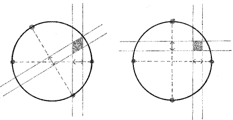
Figure 1: Quantum state tomography for a real qubit (a ‘rebit’), using pairs of bases. The statistics of each measurement determine the position of the density matrix only up to a statistical spread. Choosing the two bases representing the measurement to be unbiased—this is done for the rebit on the right—will minimize the resulting uncertainty (represented by the shaded area). Readers who recall Figure 2.11 will realize that we suppress some complications here.

MUB have numerous other applications, notably to quantum cryptography. The original BB84 protocol for quantum key distribution BB84 used a pair of qubit MUB. Going to larger sets of MUB in higher dimensions yields further advantages CBKG02 . The bottom line is that MUB are of interest when one is trying to find or hide information. Further applications include entanglement detection in the laboratory SHBAH12 , a famous retrodiction problem EA01 ; ReWe07 , and more.

Our concern will be to find out how many MUB exist in a given dimension $N$. The answer will tell us something about the shape of the convex body of mixed quantum states. To see this, note that when $N=2$ the pure states making up the three MUB form the corners of a regular octahedron inscribed in the Bloch sphere. See Figure 2. Now let the dimension of Hilbert space be $N$. The set of mixed states has real dimension $N^{2}-1$, and it has the maximally mixed state as its natural origin. An orthonormal basis corresponds to a regular simplex $\Delta_{N-1}$ centred at the origin. It spans an $(N-1)$-dimensional plane through the origin. Using the trace inner product we find that

$$|\langle e_{i}|f_{j}\rangle|^{2}=\frac{1}{N}\hskip 14.22636pt\Rightarrow\hskip 14.22636pt\mbox{Tr}\left(|e_{i}\rangle\langle e_{i}|-\frac{1}{N}{\mathbbm{1}}\right)\left(|f_{j}\rangle\langle f_{j}|-\frac{1}{N}{\mathbbm{1}}\right)=0\ .$$ (44)

Hence the condition that two such simplices represent a pair of MUB translates into the condition that the two $(N-1)$-planes be totally orthogonal, in the sense that every Bloch vector in one of them is orthogonal to every Bloch vector in the other. But the central equation of this section, namely (43), implies that there is room for at most $N+1$ totally orthogonal $(N-1)$-planes. It follows that there can exist at most $N+1$ MUB. But it does not at all follow that this many MUB actually exist. Our collection of $N+1$ simplices form an interesting convex polytope with $N(N+1)$ vertices, and what we are asking is whether this complementarity polytope can be inscribed into the convex body ${\cal M}^{(N)}$ of density matrices. In fact, given our caricature of this body, as the stitching found on a tennis ball (Section 8.6), this does seem a little unlikely (unless $N=2$).

Anyway a set of $N+1$ MUB in $N$ dimensions is referred to as a complete set. Do such sets exist? If we think of a basis as given by the column vectors of a unitary matrix, and if the basis is to be unbiased relative to the computational basis, then that unitary matrix must be a complex Hadamard matrix. Classifying pairs of MUB is equivalent to classifying such matrices. In Section IV we saw that they exist for all $N$, often in abundance. To be specific, let the identity matrix and the Fourier matrix (36) represent a pair of MUB. Can we find a third basis, unbiased with respect to both? Using $N=3$ as an illustrative example we find that Figure 4.10 gives the story away. A column vector in a complex Hadamard matrix corresponds to a point on the maximal torus in the octant picture. The twelve column vectors

$$\left[\begin{array}[]{ccc|ccc|ccc|ccc}1&0&0&1&\omega^{2}&\omega^{2}&1&\omega&\omega&1&1&1\\ 0&1&0&\omega^{2}&1&\omega^{2}&\omega&1&\omega&1&\omega&\omega^{2}\\ 0&0&1&\omega^{2}&\omega^{2}&1&\omega&\omega&1&1&\omega^{2}&\omega\end{array}\right]$$ (45)

form four MUB, and it is clear from the picture that this is the largest number that can be found. (For convenience we did not normalize the vectors. The columns of the Fourier matrix $F$ were placed on the right.)

We multiplied the vectors in the two bases in the middle with phase factors in a way that helps to make the pattern memorable. Actually there is a bit more to it. They form circulant matrices of size 3, meaning that they can be obtained by cyclic permutations of their first row. Circulant matrices have the nice property that $F^{\dagger}CF$ is a diagonal matrix for every circulant matrix $C$.

Figure 2: a) When $N=2$ a complete set of MUB forms a regular octahedron inscribed in the Bloch sphere. Each of the bases is an eigenbasis for some element in the Weyl–Heisenberg group, represented in the figure by a $\pi$-rotation through an axis. b) A poor man’s picture of the octahedron, shown as three 1-simplices, assumed to be mutually orthogonal and to intersect only at the maximally mixed state. c) A poor man’s picture of four MUB in three dimensions—in the 8-dimensional Bloch space it consists of four 2-simplices spanning totally orthogonal subspaces, intersecting only at the maximally mixed state. Each basis is the eigenbasis of a cyclic subgroup generated by some element of the Weyl–Heisenberg group.

The picture so far is summarized in Figure 2. The key observation is that each of the bases is an eigenbasis for a cyclic subgroup of the Weyl–Heisenberg group. As it turns out this generalizes straightforwardly to all dimensions such that $N=p$, where $p$ is an odd prime. We gave a list of $N+1$ cyclic subgroups in eq. (17). Each cyclic subgroup consists of a complete set of commuting observables, and they determine an eigenbasis. We denote the $a$-th vector in the $x$-th eigenbasis as $|x,a\rangle$, and we have to solve

$$D_{0,1}|0,a\rangle=\omega^{a}|0,a\rangle\ ,\hskip 8.53581ptD_{x,1}|x,a\rangle=\omega^{a}|x,a\rangle\ ,\hskip 8.53581ptD_{-1,0}|\infty,a\rangle=\omega^{a}|\infty,a\rangle\ .$$ (46)

Here $x=1,\dots,p-1$, but in the spirit of projective geometry we can extend the range to include $0$ and $\infty$ as well. The solution, with $\{|e_{r}\rangle\}_{r=0}^{p-1}$ denoting the computational basis, is

$$|0,a\rangle=|e_{a}\rangle\ ,\hskip 8.53581pt|x,a\rangle=\frac{1}{\sqrt{p}}\sum_{r=0}^{p-1}\omega^{\frac{(r-a)^{2}}{2x}}|e_{r}\rangle\ ,\hskip 8.53581pt|\infty,a\rangle=\frac{1}{\sqrt{p}}\sum_{r=0}^{p-1}\omega^{ar}|e_{r}\rangle\ .$$ (47)

It is understood that if ‘1/2’ occurs in an exponent it denotes the inverse of 2 in arithmetic modulo $p$ (and similarly for ‘1/x’). There are $p-1$ bases presented as columns of circulant matrices, and we use $\infty$ to label the Fourier basis for a reason (Problem 12.5) One can show directly (as done in 1981 by Ivanović Iv81 , whose interest was in state tomography) that these bases form a complete set of MUB (Problem 12.6),but a simple and remarkable theorem will save us from this effort.

Interestingly there is an alternative way to construct the complete set. When $N=2$ it is clear that we can start with the eigenbasis of the group element $Z$ (say), choose a point on the equator, and then apply all the transformations effected by the Weyl–Heisenberg group. The resulting orbit will consist of $N^{2}$ points, and if the starting point is judiciously chosen they will form $N$ MUB, all of them unbiased to the eigenbasis of $Z$. Again the construction works in all prime dimensions $N=p$, and indeed the resulting complete set is equivalent to the previous one in the sense that there exists a unitary transformation taking the one to the other. This construction is due to Alltop (1980), whose interest was in radar applications Al80 . Later references have made the construction more transparent and more general Bl14 ; KlaRoe04 .

The central theorem about MUB existence is due to Bandyopadhyay, Boykin, Roychowdhury, and Vatan BBRV02 .

The BBRV theorem. A complete set of MUB exists in ${\mathbb{C}}^{N}$ if and only if there exists a unitary operator basis which can be divided into $N+1$ sets of $N$ commuting operators such that the sets have only the unit element in common.

Let us refer to unitary operator bases of this type as flowers, and the sets into which they are divided as petals. Note that it is eq. (43) that makes flowers possible. There can be at most $N$ mutually commuting orthogonal unitaries since, once they are diagonalized, the vectors defined by their diagonals must form orthogonal vectors in $N$ dimensions. The Weyl–Heisenberg groups are flowers if and only if $N$ is a prime number—as exemplified in Figure 3. So the fact that (47) gives a complete set of $N+1$ MUB whenever $N$ is prime follows from the theorem.

We prove the BBRV theorem one way. Suppose a complete set of MUB exists. We obtain a maximal set of commuting Hilbert-Schmidt orthogonal unitaries by carefully choosing $N$ unitary matrices $U_{r}$, with $r$ between $0$ and $N-1$:

$$U_{r}=\sum_{r}\omega^{ri}|e_{i}\rangle\langle e_{i}|\hskip 14.22636pt\Rightarrow\hskip 14.22636pt\mbox{Tr}U_{r}^{\dagger}U_{s}=\sum_{i}\omega^{i(r-s)}=N\delta_{rs}\ .$$ (48)

If the bases $\{|e_{i}\rangle\}_{i=0}^{N-1}$ and $\{|f_{i}\rangle\}_{i=0}^{N-1}$ are unbiased we can form two such sets, and it is easy to check that

$$V_{r}=\sum_{r}\omega^{ri}|f_{i}\rangle\langle f_{i}|\hskip 8.53581pt\Rightarrow\hskip 8.53581pt\mbox{Tr}V_{r}^{\dagger}U_{s}=\frac{1}{N}\sum_{i,j}\omega^{-ir}\omega^{js}=N\delta_{r,0}\delta_{s,0}\ .$$ (49)

Hence $U_{r}\neq V_{s}$ unless $r=s=0$. It may seem as if we have constructed two cyclic subgroups of the Weyl-Heisenberg group, but in fact we have not since we have said nothing about the phase factors that enter into the scalar products $\langle e_{i}|f_{j}\rangle$. But this is as may be. It is still clear that if we go in this way, we will obtain a flower from a collection of $N+1$ MUB. Turning this into an ‘if and only if’ statement is not very hard BBRV02 .

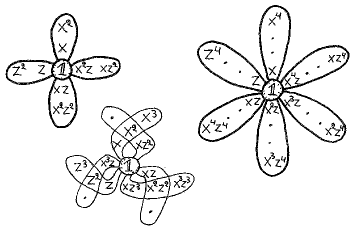
Figure 3: For $N=3$ and $5$ the cyclic subgroups of the Weyl-Heisenberg group form a flower. For $N=4$ the petals get in each other’s way and the construction fails.

We have found flowers in all prime dimensions. What about $N=4$? At this point we recall the Mermin square (5.61).It defines (as it must, if one looks at the proof of the BBRV theorem) two distinct triplets of MUB. It turns out, however, that these are examples of unextendible sets of MUB, that cannot be completed to complete sets (a fact that can be ascertained without calculations, if the reader has the prerequisites needed to solve Problem 12.7. A more constructive observation is that the operators occurring in the square belong to the 2–partite Heisenberg group $H(2)\times H(2)$. This group is also a unitary operator basis, and it contains no less than 15 maximal abelian subgroups, or petals in our language. Denoting the elements of the collineation group of $H(2)$ as $X=\sigma_{x},\ Y=\sigma_{y},\ Z=\sigma_{z}$, and the elements of the 2–partite group as (say) $XY=X\otimes Y$, we label the petals as

$$\begin{array}[]{lll}1=\{{\mathbbm{1}}Z,Z{\mathbbm{1}},ZZ\}&2=\{X{\mathbbm{1}},{\mathbbm{1}}X,XX\}&3=\{XZ,ZX,YY\}\\ 4=\{{\mathbbm{1}}Z,X{\mathbbm{1}},XZ\}&5=\{Z{\mathbbm{1}},{\mathbbm{1}}X,ZX\}&6=\{ZZ,XX,YY\}\end{array}$$ (50)

(these are the petals occurring in the Mermin square), and

$$\begin{array}[]{lll}\ 7=\{{\mathbbm{1}}Z,Y{\mathbbm{1}},YZ\}&\ 8=\{Z{\mathbbm{1}},{\mathbbm{1}}Y,ZY\}&\ 9=\{X{\mathbbm{1}},{\mathbbm{1}}Y,XY\}\\ 10=\{{\mathbbm{1}}X,Y{\mathbbm{1}},YX\}&11=\{{\mathbbm{1}}Y,Y{\mathbbm{1}},YY\}&12=\{XY,YX,ZZ\}\\ 13=\{XZ,YX,ZY\}&14=\{XY,YZ,ZX\}&15=\{XX,YZ,ZY\}.\end{array}$$ (51)

After careful inspection one finds that the unitary operator basis can be divided into disjoint petals in 6 distinct ways, namely

$$\begin{array}[]{lll}\{1,2,11,13,14\}&\{4,6,8,10,15\}&\{2,3,7,8,12\}\\ \{1,3,9,10,15\}&\{4,5,11,12,14\}&\{5,6,7,9,13\}\ .\end{array}$$ (52)

So we have six flowers, each of which contains exactly two Mermin petals (not by accident, as Problem 12.7 reveals). The pattern is summarized in Figure 4.

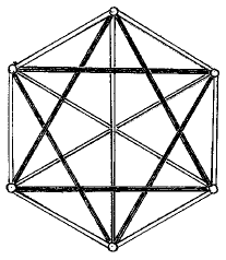
Figure 4: The 15 edges of the complete 6-graph represent the bases defined by the altogether 15 maximal abelian subgroups of $H(2)\times H(2)$. The vertices are complete sets of MUB. The 5 edges meeting at a vertex represent the bases in that set. The bases occurring in the Mermin square are painted black.

This construction can be generalized to any prime power dimension $N=p^{K}$, The multipartite Heisenberg group $H(p)^{\otimes K}$ gives many interlocking flowers, and hence many complete sets of MUB. The finite Galois fields are useful here: the formulas can be made to look quite similar to (47), except that the field theoretic trace is used in the exponents of $\omega$. We do not go into details here, but mention only that Complete sets of MUB were constructed for prime power dimensions by Wootters and Fields (1989) WF89 . Calderbank et al. CCKS97 gave a more complete list, still relying on Heisenberg groups. All known constructions are unitarily equivalent to one on their list GoRo09 .

The question whether all complete sets of MUB can be transformed into each other by means of some unitary transformation arises at this point. It is a difficult one. For $N\leq 5$ one can show that all complete sets are unitarily equivalent to each other, but for $N=2^{5}$ this is no longer true. In this case the 5–partite Heisenberg group can be partitioned into flowers in several unitarily inequivalent ways. This was noted by Kantor, who has also reviewed the full story Kan12 .

What about dimensions that are not prime powers? Unitary operator bases exist in abundance, and defy classification, so it is not easy to judge whether there may be a flower among them. Nice error bases are easier to deal with (because groups can classified). There are Heisenberg groups in every dimension, and if the dimension is $N=p_{1}^{K_{1}}p_{2}^{K_{2}}\dots p_{n}^{K_{n}}$ one can use them to construct ${\rm min}_{i}(p_{i}^{K_{i}})+1$ MUB in the composite dimension $N$ KlaRoe04 ; Zau99 . What is more, it is known that this is the largest number one can obtain from the partitioning of any nice error basis into petals Asc07 . However, the story does not end there, because—making use of the combinatorial concepts introduced in the next section—one can show that in certain square dimensions larger, but still incomplete, sets do exist. In particular, in dimension $N=26^{2}=2^{2}13^{2}$ group theory would suggest at most 5 MUB, but Wocjan and Beth found a set of 6 MUB. Moreover, in square dimensions $N=m^{2}$ the number of MUB grows at least as fast as $m^{1/14.8}$ (with finitely many exceptions) WoBe05 .

This leaves us somewhat at sea. We do not know whether a complete set of MUB exists if the dimension is $N=6,10,12,\dots$. How is the question to be settled? Numerical computer searches with carefully defined error bounds could settle the matter in low dimensions, but the only case that has been investigated in any depth is that of $N=6$. In this case there is convincing evidence that at most 3 MUB can be found, but still no proof. (Especially convincing evidence was found by Brierley and Weigert BrW08 , Jaming et al. JMMSW09 , and Raynal et al. RLE11 . See also Grassl Gr04 , who studies the set of vectors unbiased relative to both the computational and Fourier basis. There are 48 such vectors). And $N=6$ may be a very special case.

A close relative of the MUB existence problem arises in Lie algebra theory, and is unsolved there as well. But at least it received a nice name: the Winnie–the–Pooh problem. The reason cannot be fully rendered into English KT94 .

One can imagine that it has do with harmonic (Fourier) analysis Ma12 . Or perhaps with symplectic topology: there exists an elegant geometrical theorem which says that given any two bases in ${\mathbb{C}}^{N}$, not necessarily unbiased, there always exist at least $2^{N-1}$ vectors that are unbiased relative to both bases. But there is no information about whether these vectors form orthogonal bases (and in non–generic cases the vectors may coincide). (See AB15 for a description of this theorem, and Ar00 for a description of this area of mathematics). We offer these suggestions as hints, and return to a brief summary of known facts at the end of Section VI. Then we will have introduced some combinatorial ideas which—whether they have any connection to the MUB existence problem or not—have a number of applications to physics.

VI Finite geometries and discrete Wigner functions

A combinatorial structure underlying the usefulness of mutually unbiased bases is that of finite affine planes. A finite plane is just like an ordinary plane, but the number of its points is finite. A finite affine plane contains lines too, which by definition are subsets of the set of points. It is required that for any pair of points there is a unique line containing them. It is also required that for every point not contained in a given line there exists a unique line having no point in common with the given line. (Devoted students of Euclid will recognize this as the Parallel Axiom, and will also recognize that disjoint lines deserve to be called parallel.) Finally, to avoid degenerate cases, it is required that there are at least two points in each line, and that there are at least two distinct lines. With these three axioms one can prove that two lines intersect either exactly once or not at all, and also that for every finite affine plane there exists an integer $N$ such that

(i) there are $N^{2}$ points,

(ii) each line contains $N$ points,

(iii) each point is contained in $N+1$ lines,

(iv) and there are altogether $N+1$ sets of $N$ disjoint lines.

The proofs of these theorems are exercises in pure combinatorics Ben95 , and appear at first glance quite unconnected to the geometry of quantum states.

It is much harder to decide whether a finite affine plane of order $N$ actually exists. If $N$ is a power of a prime number finite planes can be constructed using coordinates, just like the ordinary plane (where lines are defined by linear equations in the coordinates that label the points), with the difference that the coordinates are elements of a finite field of order $N$. Thus a point is given by a pair $(x,y)$, where $x$, $y$ belong to the finite field, and a line consists of all points obeying either $y=ax+b$ or $x=c$, where $a,b,c$ belong to the field. This is not quite the end of the story of the finite affine planes because examples have been constructed that do not rely on finite fields, but the order $N$ of all these examples is a power of some prime number. Whether there exist finite affine planes for any other $N$ is not known.

Let us go a little deeper into the combinatorics, before we explain what it has to do with us. A finite plane can clearly be thought of as a grid of $N^{2}$ points, and its rows and columns provide us with two sets of $N$ disjoint or parallel lines, such that each line in one of the sets intersect each line in the other set exactly once. But what of the next set of $N$ parallel lines? We can label its lines with letters from an alphabet containing $N$ symbols, and the requirement that any two lines meet at most once translates into the observation that finding the third set is equivalent to finding a Latin square. As we saw in Section IV, there are many Latin squares to choose from. The difficulty comes in the next step, when we ask for two Latin squares describing two different sets of parallel lines. Use Latin letters as the alphabet for the first, and Greek letters for the second. Then each point in the array will be supplied with a pair of letters, one Latin and one Greek. Since two lines are forbidden to meet more than once a given pair of letters, such as $(A,\alpha)$ or $(B,\gamma)$, is allowed to occur only once in the array. In other words the letters from the two alphabets serve as alternative coordinates for the array. Pairs of Latin squares enjoying this property are known as Graeco-Latin or orthogonal Latin squares. For $N=3$ it is easy to find Graeco-Latin pairs, such as

$$\left(\ \ \begin{array}[]{|c|c|c|}\hline\cr A&B&C\\ \hline\cr B&C&A\\ \hline\cr C&A&B\\ \hline\cr\end{array}\ ,\ \begin{array}[]{|c|c|c|}\hline\cr\alpha&\beta&\gamma\\ \hline\cr\gamma&\alpha&\beta\\ \hline\cr\beta&\gamma&\alpha\\ \hline\cr\end{array}\ \ \right)\ =\ \begin{array}[]{|c|c|c|}\hline\cr{A\alpha}&B\beta&{C\gamma}\\ \hline\cr{B\gamma}&C\alpha&{A\beta}\\ \hline\cr{C\beta}&A\gamma&{B\alpha}\\ \hline\cr\end{array}\ .$$ (53)

An example for $N=4$, using alphabets that may appeal to bridge players, is

$${\small\begin{array}[]{|cccc|}\hline\cr{A\spadesuit}&K\clubsuit&{Q\diamondsuit}&J\heartsuit\\ {K\heartsuit}&A\diamondsuit&{J\clubsuit}&Q\spadesuit\\ {Q\clubsuit}&J\spadesuit&{A\heartsuit}&K\diamondsuit\\ J\diamondsuit&Q\heartsuit&K\spadesuit&A\clubsuit\\ \hline\cr\end{array}}\ .$$ (54)

Graeco-Latin pairs can be found for all choices of $N>2$ except (famously) $N=6$. This is so even though Table 2 shows that there is a very large supply of Latin squares for $N=6$. The story behind these non-existence results goes back to Euler, who was concerned with arranging 36 officers belonging to 6 regiments, 6 ranks, and 6 arms, in a square.

To define a complete affine plane, with $N+1$ sets of parallel lines, requires us to find a set of $N-1$ mutually orthogonal Latin squares, or MOLS. For $N=6$ and $N=10$ this is impossible, and in fact an infinite number of possibilities (beginning with $N=6$) are ruled out by the Bruck-Ryser theorem, which says that if an affine plane of order $N$ exists, and if $N=1$ or 2 modulo 4, then $N$ must be the sum of two squares. Note that 10 is a sum of two squares, but this case has been ruled out by different means. Lam describes the computer based non-existence proof for $N=10$ in a thought-provoking way Lam91 .

If $N=p^{k}$ for some prime number $p$ a solution can easily be found using analytic geometry over finite fields. There remain an infinite number of instances, beginning with $N=12$, for which the existence of a finite affine plane is an open question. See the books by Bennett Ben95 , and Stinson Sti04 , for more information, and for proofs of the statements we have made so far.

At this point we recall that complete sets of MUB exist when $N=p^{k}$, but quite possibly not otherwise. Moreover such a complete set is naturally described by $N+1$ sets of $N$ vectors. The total number of vectors is the same as the number of lines in a finite affine plane, so the question is if we can somehow associate $N^{2}$ ‘points’ to a complete set of MUB, in such a way that the incidence structure of the finite affine plane becomes useful. One way to do this is to start with the picture of a complete set of MUB as a polytope in Bloch space. We do not have to assume that a complete set of MUB exists. We simply introduce $N(N+1)$ Hermitian matrices $P_{\nu}$ of unit trace, denoted $P_{v}$, and obeying

$$\mbox{Tr}P_{v}P_{v^{\prime}}=\left\{\begin{array}[]{lll}1&\mbox{if}&v=v^{\prime}\\ 1/N&\mbox{if}&v\ \mbox{and}\ v^{\prime}\ \mbox{sit in different planes}\\ 0&\mbox{if}&v\neq v^{\prime}\ \mbox{sit in the same plane}\end{array}\right.$$ (55)

The condition that Tr$P_{v}^{2}=1$ ensures that $P_{v}$ lies on the outsphere of the set of quantum states. If their eigenvalues are non-negative these are projectors, and then they actually are quantum states, but this is not needed for the definition of the polytope. To understand the face structure of the polytope we begin by noting that the convex hull of one vertex from each of the $N+1$ individual simplices forms a face. (This is fairly obvious, and anyway we are just about to prove it.) Using the matrix representation of the vertices we can then form the Hermitian unit trace matrix

$$A_{f}=\sum_{\rm face}P_{v}-{\mathbbm{1}}\ ,$$ (56)

where the sum runs over the $N+1$ vertices in the face. This is called a face point operator (later to be subtly renamed as a phase point operator). If $N=3$ we can think of it pictorially as $\triangle{\ }^{\bullet}\hskip 6.54413pt\triangle{\ }^{\bullet}\hskip 6.54413pt\triangle{\ }^{\bullet}\hskip 6.54413pt\triangle{\ }^{\bullet}\hskip 7.11317pt$, say—each triangle represents a basis. See Figure 2. It is easy to see that $0\leq\mbox{Tr}\rho A_{f}\leq 1$ for any matrix $\rho$ that lies in the complementarity polytope, which means that the latter is confined between two parallel hyperplanes. There is a facet defined by $\mbox{Tr}\rho A_{f}=0$ (pictorially, this would be $\triangle{\ }_{\bullet}{\ }_{\bullet}\hskip 6.54413pt\triangle{\ }_{\bullet}{\ }_{\bullet}\hskip 6.54413pt\triangle{\ }_{\bullet}{\ }_{\bullet}\hskip 6.54413pt\triangle{\ }_{\bullet}{\ }_{\bullet}\hskip 2.84526pt$) and an opposing face containing one vertex from each simplex. Every vertex is included in one of these two faces. There are $N^{N+1}$ operators $A_{f}$ altogether, and equally many facets.

The idea is to select $N^{2}$ phase point operators and use them to represent the points of an affine plane. The $N+1$ vertices $P_{\nu}$ that appear in the sum (56) are to be regarded as the $N+1$ lines passing through the point $A_{f}$. A set of $N$ parallel lines in the affine plane will represent a complete set of orthonormal projectors.

Figure 5: All the points on a line determine a $P_{v}$, and all the lines through a point determine an $A_{ij}$. In fact we are illustrating eqs. (60).

To do so, recall that each $A_{f}$ is defined by picking one $P_{v}$ from each basis. Let us begin by making all possible choices from the first two, and arrange them in an array:

$$\begin{array}[]{ccccc}\triangle{\ }^{\bullet}\hskip 9.10486pt\triangle{\ }_{\bullet}\hskip 5.69054pt\triangle\ \triangle&&\triangle{\ }_{\bullet}\hskip 11.38109pt\triangle{\ }_{\bullet}\hskip 5.69054pt\triangle\ \triangle&&\triangle{\ }_{\bullet}\hskip 5.69054pt\triangle{\ }_{\bullet}\hskip 5.69054pt\triangle\ \triangle\\ &&&&\\ \triangle{\ }^{\bullet}\hskip 9.10486pt\triangle{\ }_{\bullet}\hskip 11.95013pt\triangle\ \triangle&&\triangle{\ }_{\bullet}\hskip 11.95013pt\triangle{\ }_{\bullet}\hskip 11.95013pt\triangle\ \triangle&&\triangle{\ }_{\bullet}\hskip 5.69054pt\triangle{\ }_{\bullet}\hskip 11.95013pt\triangle\ \triangle\\ &&&&\\ \triangle{\ }^{\bullet}\hskip 9.10486pt\triangle{\ }^{\bullet}\hskip 9.10486pt\triangle\ \triangle&&\triangle{\ }_{\bullet}\hskip 11.38109pt\triangle{\ }^{\bullet}\hskip 9.10486pt\triangle\ \triangle&&\triangle{\ }_{\bullet}\hskip 5.69054pt\triangle{\ }^{\bullet}\hskip 9.10486pt\triangle\ \triangle\end{array}$$ (57)

We set $N=3$—enough to make the idea come through—in this illustration. Thus the $N+1$ simplices in the totally orthogonal $(N-1)$-planes appear as four triangles, two of which have been used up to make the array. We use the vertices of the remaining $N-1$ simplices to label the lines in the remaining $N-1$ pencils of parallel lines. To ensure that non-parallel lines intersect exactly once a pair such as $\triangle{\ }_{\bullet}\hskip 5.69054pt\triangle{\ }_{\bullet}\$ (picked from any two out of the four triangles) must occur exactly once in the array. This problem can be solved because an affine plane of order $N$ is presumed to exist. One solution is

$$\begin{array}[]{ccccc}\triangle{\ }^{\bullet}\hskip 9.10486pt\triangle{\ }_{\bullet}\hskip 5.69054pt\triangle{\ }_{\bullet}\hskip 11.38109pt\triangle{\ }_{\bullet}&&\triangle{\ }_{\bullet}\hskip 11.38109pt\triangle{\ }_{\bullet}\hskip 5.69054pt\triangle{\ }_{\bullet}\hskip 5.69054pt\triangle{\ }^{\bullet}&&\triangle{\ }_{\bullet}\hskip 5.69054pt\triangle{\ }_{\bullet}\hskip 5.69054pt\triangle{\ }^{\bullet}\hskip 9.10486pt\triangle{\ }_{\bullet}\\ &&&&\\ \triangle{\ }^{\bullet}\hskip 9.10486pt\triangle{\ }_{\bullet}\hskip 11.95013pt\triangle{\ }_{\bullet}\hskip 5.69054pt\triangle{\ }_{\bullet}&&\triangle{\ }_{\bullet}\hskip 11.95013pt\triangle{\ }_{\bullet}\hskip 11.95013pt\triangle{\ }^{\bullet}\hskip 9.10486pt\triangle{\ }_{\bullet}&&\triangle{\ }_{\bullet}\hskip 5.69054pt\triangle{\ }_{\bullet}\hskip 11.95013pt\triangle{\ }_{\bullet}\hskip 11.38109pt\triangle{\ }^{\bullet}\\ &&&&\\ \triangle{\ }^{\bullet}\hskip 9.10486pt\triangle{\ }^{\bullet}\hskip 9.10486pt\triangle{\ }^{\bullet}\hskip 9.10486pt\triangle{\ }^{\bullet}&&\triangle{\ }_{\bullet}\hskip 11.38109pt\triangle{\ }^{\bullet}\hskip 9.10486pt\triangle{\ }_{\bullet}\hskip 11.38109pt\triangle{\ }_{\bullet}&&\ \ \triangle{\ }_{\bullet}\hskip 5.69054pt\triangle{\ }^{\bullet}\hskip 9.10486pt\triangle{\ }_{\bullet}\hskip 5.69054pt\triangle{\ }_{\bullet}\end{array}$$ (58)

We have now singled out $N^{2}$ face point operators for attention, and the combinatorics of the affine plane guarantees that any pair of them have exactly one $P_{v}$ in common. Equation (55) then enables us to compute that

$$\mbox{Tr}A_{f}A_{f^{\prime}}=N\delta_{f,f^{\prime}}\ .$$ (59)

This is a regular simplex in dimension $N^{2}-1$.

We used only $N^{2}$ out of the $N^{N+1}$ face point operators for this construction, but a little reflection shows that the set of all of them can be divided into $N^{N-1}$ disjoint face point operator simplices. In effect we have inscribed the complementarity polytope into this many regular simplices, which is an interesting datum about the former. Each such simplex forms an orthogonal operator basis, although not necessarily a unitary operator basis. Let us focus on one of them, and label the operators occurring in it as $A_{i,j}$. It is easy to see that eq. (56) can be rewritten (in the language of the affine plane), and supplemented, so that we have the two equations

$$P_{v}=\frac{1}{N}\sum_{{\rm line}\ v}A_{i,j}\ ,\hskip 28.45274ptA_{i,j}=\sum_{{\rm point}\ (i,j)}P_{v}-{\mathbbm{1}}\ .$$ (60)

The summations extend through all points on the line, respectively all lines passing through the point. Using the fact that the phase point operators form an operator basis we can then define a discrete Wigner function by

$$W_{i,j}=\frac{1}{N}\mbox{Tr}A_{i,j}\rho\ .$$ (61)

Knowledge of the $N^{2}$ real numbers $W_{i,j}$ is equivalent to knowledge of the density matrix $\rho$. Each line in the affine plane is now associated with the number

$$p_{v}=\sum_{{\rm line}\ v}W_{i,j}=\mbox{Tr}P_{v}\rho\ .$$ (62)

Clearly the sum of these numbers over a pencil of parallel lines equals unity. However, so far we have used only the combinatorics of the complementarity polytope, and we have no right to expect that the operators $P_{v}$ have positive spectra. They will be projectors onto pure states if and only if the complementarity polytope has been inscribed into the set of density matrices, which is a difficult thing to achieve. If it is achieved we conclude that $p_{v}\geq 0$, and then we have an elegant discrete Wigner function—giving all the correct marginals—on our hands Wo87 . It will receive further polish in the next section.

Meanwhile, now that we have the concepts of mutually orthogonal Latin squares and finite planes on the table, we can discuss some interesting but rather abstract analogies to the MUB existence problem. Fix $N=p_{1}^{K_{1}}p_{2}^{K_{2}}\dots p_{n}^{K_{n}}$. Let $\#_{\rm MUB}$ be the number of MUB, and let $\#_{\rm MOLS}$ be the number of MOLS. (We need only $N-1$ MOLS to construct a finite affine plane.) Then

$$\begin{array}[]{l}{\rm min}_{i}(p_{i}^{K_{i}})-1\leq\#_{\rm MOLS}\leq N-1\\ \\ {\rm min}_{i}(p_{i}^{K_{i}})+1\leq\#_{\rm MUB}\leq N+1\ .\end{array}$$ (63)

The lower bound for MOLS is known as the MacNeish bound Ma21 . Moreover, if $N=6$, we know that Latin squares cannot occur in orthogonal pairs, and we believe that there exist only three MUB. Finally, it is known that if there exist $N-2$ MOLS there necessarily exist $N-1$ MOLS, and if there exist $N$ MUB there necessarily exist $N+1$ MUB We13 . This certainly encourages the speculation that the existence problem for finite affine planes is related to the existence problem for complete sets of MUB in some unknown way. However, the idea fades a little if one looks carefully into the details PPGB10 ; WD10 .

VII Clifford groups and stabilizer states

To go deeper into the subject we need to introduce the Clifford group. We use the displacement operators $D_{\bf p}$ from Section II to describe the Weyl–Heisenberg group. By definition the Clifford group consists of all unitary operators $U$ such that

$$UD_{\bf p}U^{-1}\sim D_{f({\bf p})}\ ,$$ (64)

where $\sim$ means ‘equal up to phase factors’. (Phase factors will appear if $U$ itself is a displacement operator, which is allowed.) Thus we ask for unitaries that permute the displacement operators, so that the conjugate of an element of the Weyl-Heisenberg group is again a member of the Weyl–Heisenberg group. The technical term for this is that the Clifford group is the normalizer of the Weyl-Heisenberg group within the unitary group, or that the Weyl–Heisenberg group is an invariant subgroup of the Clifford group. If we change $H(N)$ into a non-isomorphic multipartite Heisenberg group we obtain another Clifford group, but at first we stick with $H(N)$. (The origin of the name ‘Clifford group’ is a little unclear to us. It seems to be connected to Clifford’s gamma matrices rather than to Clifford himself BRW60 ).

The hard part of the argument is to show that

$$U_{G}D_{\bf p}U^{-1}_{G}\sim D_{G{\bf p}}\ ,$$ (65)

where $G$ is a two-by-two matrix with entries in ${\mathbbm{Z}}_{\bar{N}}$, the point being that the map ${\bf p}\rightarrow f({\bf p})$ has to be linear App05 . We take this on trust here. To see the consequences we return to the group law (12). In the exponent of the phase factor we encounter the symplectic form

$$\Omega({\bf p},{\bf q})=p_{2}q_{1}-p_{1}q_{2}\ .$$ (66)

When strict equality holds in eq. (65) it follows from the group law that

$$U_{G}D_{\bf p}D_{\bf q}U^{-1}_{G}=\tau^{\Omega({\bf p},{\bf q})}UD_{{\bf p}+{\bf q}}U^{-1}_{G}\hskip 5.69054pt\Rightarrow\hskip 5.69054ptD_{G{\bf p}}D_{G{\bf q}}=\tau^{\Omega({\bf p},{\bf q})}D_{G({\bf p}+{\bf q})}\ .$$ (67)

On the other hand we know that

$$D_{G{\bf p}}D_{G{\bf q}}=\tau^{\Omega(G{\bf p},G{\bf q})}D_{G({\bf p}+{\bf q})}\ .$$ (68)

Consistency requires that

$$\Omega({\bf p},{\bf q})=\Omega(G{\bf p},G{\bf q})\hskip 11.38109pt\mbox{mod}\ \bar{N}\ .$$ (69)

The two by two matrix $G$ must leave the symplectic form invariant. The arithmetic in the exponent is modulo $\bar{N}$, where $\bar{N}=N$ if $N$ is odd and $\bar{N}=2N$ if $N$ is even. We deplored this unfortunate complication in even dimensions already in Section II.

Let us work with explicit matrices

$$\Omega=\left(\begin{array}[]{cc}0&-1\\ 1&0\end{array}\right)\ ,\hskip 22.76219ptG=\left(\begin{array}[]{cc}\alpha&\beta\\ \gamma&\delta\end{array}\right)\ ,\hskip 22.76219pt\alpha,\beta,\gamma,\delta\in{\mathbbm{Z}}_{\bar{N}}\ .$$ (70)

Then eq. (69) says that

$$\left(\begin{array}[]{cc}0&-1\\ 1&0\end{array}\right)=\left(\begin{array}[]{cc}0&-\alpha\delta+\beta\gamma\\ \alpha\delta-\beta\gamma&0\end{array}\right)\ .$$ (71)

Hence the matrix $G$ must have determinant equal to 1 modulo $\bar{N}$. Such matrices form the group $SL(2,{\mathbbm{Z}}_{\bar{N}})$, where ${\mathbbm{Z}}_{\bar{N}}$ stands for the ring of integers modulo $\bar{N}$. It is also known as a symplectic group, because it leaves the symplectic form invariant.

The full structure of the Clifford group $C(N)$ is complicated by the phase factors, and rather difficult to describe in general. Things are much simpler when $\bar{N}=N$ is odd, so let us restrict our description to this case. (A complete, and clear, account of the general case is given by Appleby App05 ). Then the symplectic group is a subgroup of the Clifford group. Another subgroup is evidently the Weyl–Heisenberg group itself. Moreover, if we consider the Clifford group modulo its centre, $C(N)/I(N)$, that is to say if we identify group elements differing only by phase factors—which we would naturally do if we are interested only in how it transforms the quantum states—then we find that $C(N)/I(N)$ is a semi-direct product of the symplectic rotations given by $SL(2,{\mathbbm{Z}}_{N})$ and the translations given by $H(N)$ modulo its centre.

In every case—also when $N$ is even—the unitary representation of the Clifford group is uniquely determined by the unitary representation of the Weyl-Heisenberg group. The easiest case to describe is that when $N$ is an odd prime number $p$. Then the symplectic group is defined over the finite field ${\mathbbm{Z}}_{p}$ consisting of integers modulo $p$, and it contains $p(p^{2}-1)$ elements altogether. Insisting that there exists a unitary matrix $U_{G}$ such that $U_{G}D_{\bf p}U_{G}^{-1}=D_{G{\bf p}}$ we are led to the representation

$$G=\left(\begin{array}[]{cc}\alpha&\beta\\ \gamma&\delta\end{array}\right)\hskip 2.84526pt\rightarrow\hskip 2.84526pt\left\{\begin{array}[]{ll}U_{G}=\frac{e^{i\theta}}{\sqrt{p}}\sum_{i,j}\omega^{\frac{1}{2\beta}(\delta i^{2}-2ij+\alpha j^{2})}|i\rangle\langle j|&\ \beta\neq 0\\ \\ U_{G}=\pm\sum_{j}\omega^{\frac{\alpha\gamma}{2}j^{2}}|\alpha j\rangle\langle j|&\ \beta=0\ .\end{array}\right.$$ (72)

In these formulas ‘$1/\beta$’ stands for the multiplicative inverse of the integer $\beta$ in arithmetic modulo $p$ (and since $1/2$ occurs it is obvious that special measures must be taken if $p=2$). An overall phase factor is left undetermined: it can be pinned down by insisting on a faithful representation of the group Neu02 ; App09 , but in many situations it is not needed. It is noteworthy that the representation matrices are either complex Hadamard matrices, or monomial matrices. It is interesting to see how they act on the set of mutually unbiased bases. In the affine plane a symplectic transformation takes lines to lines, and indeed parallel lines to parallel lines. If one works this out one finds that the symplectic group acts like Möbius transformations on a projective line whose points are the individual bases. See Problem 12.5.

Even though $N=2$ is even, it is the easiest case to understand. The collineation group $C(2)/I(2)$ is just the group of rotations that transforms the polytope formed by the MUB states into itself, or in other words it is the symmetry group $S_{4}$ of the octahedron. In higher prime dimensions the Clifford group yields only a small subgroup of the symmetry group of the complementarity polytope. When $N$ is a composite number, and especially if $N$ is an even composite number, there are some significant complications for which we refer elsewhere App05 . These complications do sit in the background in Section IX, where the relevant group is the extended Clifford group obtained by allowing also two-by-two matrices of determinant $\pm 1$. In Hilbert space this doubling of the group is achieved by representing the extra group elements by anti-unitary transformations App05 .

To cover MUB in prime power dimensions we need to generalize in a different direction. The relevant Heisenberg group is the multipartite Heisenberg group. We can still define the Clifford group as the normalizer of this Heisenberg group. We recall that the latter contains many maximal abelian subgroups, and we refer to the joint eigenvectors of these subgroups as stabilizer states. The Clifford group acts by permuting the stabilizer states, and every such permutation can be built as a sequence of operations on no more than two qubits (or quNits as the case may be) at a time. In one standard blueprint for universal quantum computing Go97 , the quantum computer is able to perform such permutations in a fault–tolerant way, and the stabilizer states play a role reminiscent of that played by the separable states (to be defined in Chapter 16) in quantum communication.

The total number $M$ of stabilizer states in $N=p^{K}$ dimensions is

$$M=p^{K}\prod_{i=1}^{K}(p^{i}+1)\ .$$ (73)

Dividing out a factor $p^{K}$ we obtain the number of maximal abelian subgroups of the Heisenberg group. In dimension $N=2^{2}$ there are altogether 60 stabilizer states forming 15 bases and 6 interlocking complete sets of MUB, because there are 6 different ways in which the group $H(2)\times H(2)$ can be displayed as a flower. See Figure 4.

The story in higher dimensions is complicated by the appearance of complete sets that fail to be unitarily equivalent to each other. We must refer elsewhere for the details Kan12 , but it is worth remarking that, for the ‘canonical’ choice of a complete set written down by Ivanović Iv81 and by Wootters and Fields WF89 , there exists a very interesting subgroup of the Clifford group leaving this set invariant. It is known as the restricted Clifford group App09 , and has an elegant description in terms of finite fields. Moreover (with an exception in dimension 3) the set of vectors that make up this set of MUB is distinguished by the property that it provides the smallest orbit under this group Zh15 . For both Clifford groups, the quotient of their collineation groups with the discrete translation group provided by their Heisenberg groups is a symplectic group. If we start with the full Clifford group the symplectic group acts on a $2K$-dimensional vector space over ${\mathbbm{Z}}_{p}$, while in the case of the restricted Clifford group it can be identified with the group $SL(2,{\mathbbm{F}}_{p^{K}})$ acting on a 2-dimensional vector space over the finite field ${\mathbbm{F}}_{p^{K}}=GF(p^{K})$ Gro06 .

Armed with these group theoretical facts we can return to the subject of discrete Wigner functions. If we are in a prime power dimension it is evident that we can produce a phase point operator simplex by choosing any phase point operator $A_{f}$, and act on it with the appropriate Heisenberg group. But we can ask for more. We can ask for a phase point operator simplex that transforms into itself when acted on by the Clifford group. If we succeed, we will have an affine plane that behaves like a true phase space, since it will be equipped with a symplectic structure. This turns out to be possible in odd prime power dimensions, but not quite possible when the dimension is even. We confine ourselves to odd prime dimensions here. Then the Clifford group contains a unique element of order two, whose unitary representative we call $A_{0,0}$ Wo87 . Using eq. (72) it is

$$G=\left(\begin{array}[]{rr}-1&0\\ 0&-1\end{array}\right)\hskip 14.22636pt\Rightarrow\hskip 14.22636ptA_{0,0}=U_{G}=\sum_{i=0}^{N-1}|N-i\rangle\langle i|\ .$$ (74)

By the way we observe that $A_{0,0}^{2}=F$, where $F$ is the Fourier matrix. Making use of eqs. (15-16) we find

$$A_{0,0}=\sum_{r,s}D_{r,s}\ .$$ (75)

To perform this sum, split it into a sum over the $N+1$ maximal abelian subgroups and subtract ${\mathbbm{1}}$ to avoid overcounting. Diagonalize each individual generator of these subgroups, say

$$D_{0,1}=Z=\omega^{a}\sum_{a}|0,a\rangle\langle 0,a|\hskip 14.22636pt\Rightarrow\hskip 14.22636pt\sum_{i=0}^{N-1}Z^{i}=N|0,0\rangle\langle 0,0|\ .$$ (76)

All subgroups work the same way, so this is enough. We conclude that

$$A_{0,0}=\sum_{z}|z,0\rangle\langle z,0|-{\mathbbm{1}}\ .$$ (77)

(The range of the label $z$ is extended to cover also the bases that we have labelled by $0$ and $\infty$.) Since we are picking one projector from each of the $N+1$ bases this is in fact a phase point operator.

Starting from $A_{0,0}$ we can build a set of $N^{2}$ order two phase point operators

$$A_{r,s}=D_{r,s}AD_{r,s}^{-1}\ .$$ (78)

Their eigenvalues are $\pm 1$, so these operators are both Hermitian and unitary. The dimension $N$ is odd, so we can write $N=2m-1$. Each phase point operator splits Hilbert space into a direct sum of eigenspaces,

$${\cal H}_{N}={\cal H}_{m}^{(+)}\oplus{\cal H}_{m-1}^{(-)}\ .$$ (79)

Altogether we have $N^{2}$ subspaces of dimension $m$, each of which contain $N+1$ MUB vectors. Conversely, one can show that each of the $N(N+1)$ MUB vectors belongs to $N$ such subspaces. This intersection pattern was said to be “une configuration très-remarquable” when it was first discovered (By Segre (1886) Se86 , who was studying elliptic normal curves. From the present point of view it was first discovered by Wootters (1987) Wo87 ).

The operators $A_{r,s}$ form a phase point operator simplex which enjoys the twin advantages of being both a unitary operator basis and an orbit under the Clifford group. A very satisfactory discrete Wigner function can be obtained from it Wo87 ; Gro06 . The situation in even prime power dimensions is somewhat less satisfactory since covariance under the full Clifford group cannot be achieved in this case.

The set of phase point operators forms a particularly interesting unitary operator basis, existing in odd prime power dimensions only. Its symmetry group acts on it in such a way that any pair of elements can be transformed to any other pair. This is at the root of its usefulness: from it we obtain a discrete Wigner function on a phase space lacking any kind of scale, just as the ordinary symplectic vector spaces used in classical mechanics lack any kind of scale. Moreover (with two exceptions, one in dimension two and and one in dimension eight) it is uniquely singled out by this property Zh16 .

VIII Some designs

To introduce our next topic let us say something obvious. We know that

$${\mathbbm{1}}_{N}=\frac{1}{N}\sum_{i=1}^{N}|e_{i}\rangle\langle e_{i}|=\int_{{\mathbbm{C}}{\bf P}^{n}}{\rm d}\Omega_{\Psi}|\Psi\rangle\langle\Psi|\ ,$$ (80)

where ${\rm d}\Omega_{\Psi}$ is the unitarily invariant Fubini–Study measure. Let $A$ be any operator acting on ${\mathbbm{C}}^{N}$. It follows that

$$\frac{1}{N}\sum_{i=0}^{N-1}\langle e_{i}|A|e_{i}\rangle=\int_{{\mathbbm{C}}{\bf P}^{n}}{\rm d}\Omega_{\Psi}\langle\Psi|A|\Psi\rangle=\langle\langle\Psi|A|\Psi\rangle\rangle_{\rm FS}\ .$$ (81)

On the right hand side we are averaging an (admittedly special) function over all of ${\mathbbm{C}}{\bf P}^{N-1}$. On the left hand side we take the average of its values at $N$ special points. In statistical mechanics this equation allows us to evaluate the average expectation value of the energy by means of the convenient fiction that the system is in an energy eigenstate—which at first sight is not obvious at all.

To see how this can be generalized we recall the mean value theorem, which says that for every continuous function defined on the closed interval $[0,1]$ there exists a point $x$ in the interval such that

$$f(x)=\int_{0}^{1}{\rm d}sf(s)\ .$$ (82)

Although it is not obvious, this can be generalized to the case of sets of functions $f_{i}$ SeZa84 . Given such a set of functions one can always find an averaging set consisting of $K$ different points $x_{I}$ such that, for all the $f_{i}$,

$$\frac{1}{K}\sum_{I=1}^{K}f_{i}(x_{I})=\int_{0}^{1}{\rm d}sf_{i}(s)\ .$$ (83)

Of course the averaging set (and the integer $K$) will depend on the set of functions $\{f_{i}\}$ one wants to average. We can generalize even more by replacing the interval with a connected space, such as ${\mathbbm{C}}{\bf P}^{N-1}$, and by replacing the real valued functions with, say, the set Hom$(t,t)$ of all complex valued functions homogeneous of order $t$ in the homogeneous coordinates and their complex conjugates alike. (The restriction on the functions is needed in order to ensure that we get functions on ${\mathbbm{C}}{\bf P}^{N-1}$. Note that the expression $\langle\psi|A|\psi\rangle$ belongs to Hom$(1,1)$.) This too can always be achieved, with an averaging set being a collection of points represented by the unit vectors $|\Psi_{I}\rangle$, $1\leq I\leq K$, for some sufficiently large integer $K$ SeZa84 . We define a complex projective t–design, or t–design for short, as a collection of unit vectors $\{|\Psi_{I}\rangle\}_{I=1}^{K}$ such that

$$\frac{1}{K}\sum_{I=1}^{K}f(|\Psi_{I}\rangle)=\int_{{\mathbbm{C}}{\bf P}^{n}}{\rm d}\Omega_{\Psi}f(|\Psi\rangle)$$ (84)

for all polynomials $f\in\mbox{Hom}(t,t)$ with the components of the vector, and their complex conjugates, as arguments. Formulas like this are called cubature formulas, since—like quadratures—they give explicit solutions of an integral, and they are of practical interest—for many signal processing and quantum information tasks—provided that $K$ can be chosen to be reasonably small.

Eq. (81) shows that orthonormal bases are 1–designs. More generally, every POVM is a 1–design. Let us also note that functions $f\in$ Hom$(t-1,t-1)$ can be regarded as special cases of functions in Hom$(t,t)$, since they can be rewritten as $f=\langle\Psi|\Psi\rangle f\in$ Hom$(t,t)$. Hence a $t$–design is automatically a $(t-1)$–design. But how do we recognize a $t$–design when we see one?

The answer is quite simple. In eq. (7.69) we calculated the Fubini–Study average of $|\langle\Phi|\Psi\rangle|^{2t}$ for a fixed unit vector $|\Phi\rangle$. Now let $\{|\Psi_{I}\rangle\}_{I=1}^{K}$ be a $t$–design. It follows that

$$\frac{1}{K}\sum_{J}|\langle\Psi_{I}|\Psi_{J}\rangle|^{2t}=\langle|\langle\Psi_{I}|\Psi\rangle|^{2t}\rangle_{\rm FS}=\frac{t!(N-1)!}{(N-1+t)!}\ .$$ (85)

If we multiply by $1/K$ and then sum over $I$ we obtain

$$\frac{1}{K^{2}}\sum_{I,J}|\langle\Psi_{I}|\Psi_{J}\rangle|^{2t}=\frac{t!(N-1)!}{(N-1+t)!}\ .$$ (86)

We have proved one direction of the following

Design theorem. The set of unit vectors $\{|\Psi\rangle\}_{I=1}^{K}$ forms a $t$–design if and only if eq. (86) holds.

In the other direction a little more thought is needed KlaRoe05 . Take any vector $|\Psi\rangle$ in ${\mathbbm{C}}^{N}$ and construct a vector in $({\mathbbm{C}}^{N})^{\otimes t}$ by taking the tensor product of the vector with itself $t$ times. Do the same with $|\bar{\Psi}\rangle$, a vector whose components are the complex conjugates of the components, in a fixed basis, of the given vector. A final tensor product leads to the vector

$$|\Psi\rangle^{\otimes t}\otimes|\bar{\Psi}\rangle^{\otimes t}\in({\mathbbm{C}}^{N})^{\otimes 2t}\ .$$ (87)

In the given basis the components of this vector are

$$(z_{0}\dots z_{0}\bar{z}_{0}\dots\bar{z}_{0},z_{0}\dots z_{0}\bar{z}_{1}\dots\bar{z}_{1},\dots\dots,z_{n}\dots z_{n}\bar{z}_{n}\dots\bar{z}_{n})\ .$$ (88)

In fact the components consists of all possible monomials in Hom$(t,t)$. Thus, to show that a set of unit vectors forms a $t$–design it is enough to show that the vector

$$|\Phi\rangle=\frac{1}{K}\sum_{I}|\Psi_{I}\rangle^{\otimes t}\otimes|\bar{\Psi}_{I}\rangle^{\otimes t}-\int{\rm d}\Omega_{\Psi}|\Psi\rangle^{\otimes t}\otimes|\bar{\Psi}\rangle^{\otimes t}$$ (89)

is the zero vector. This will be so if its norm vanishes. We observe preliminarily that

$$\langle\Psi_{I}^{\otimes t}|\Psi_{J}^{\otimes t}\rangle=\langle\Psi_{I}|\Psi_{J}\rangle^{t}\ .$$ (90)

If we make use of the ubiquitous eq. (7.69)we find precisely that

$$||\Phi||^{2}=\frac{1}{K^{2}}\sum_{I,J}|\langle\Psi_{I}|\Psi_{J}\rangle|^{2t}-\frac{t!(N-1)!}{(N-1+t)!}\ .$$ (91)

This vanishes if and only if eq. (86) holds. But $|\Phi\rangle=0$ is a sufficient condition for a $t$–design, and the theorem is proven.

This result is closely related to the Welch bound Wel74 , which holds for every collection of $K$ vectors in ${\mathbb{C}}^{N}$. For any positive integer $t$

$${{N+t-1}\choose{t}}\sum_{I,J}|\langle x_{I}|x_{J}\rangle|^{2t}\geq\left(\sum_{I}\langle x_{I}|x_{I}\rangle^{t}\right)^{2}\ .$$ (92)

Evidently a collection of unit vectors forms a $t$-design if and only if the Welch bound is saturated. The binomial coefficient occurring here is the number of ways in which $t$ identical objects can be distributed over $N$ boxes, or equivalently it is the dimension of the symmetric subspace ${\cal H}_{\rm sym}^{\otimes t}$ of the $t$–partite Hilbert space ${\cal H}_{N}^{\otimes t}$. This is not by accident. Introduce the operator

$$F=\sum_{I}|\Psi_{I}^{\otimes t}\rangle\langle\Psi_{I}^{\otimes t}|\ .$$ (93)

It is then easy to see, keeping eq. (90) in mind, that

$$\mbox{Tr}F=\sum_{I}\langle\Psi_{I}^{\otimes t}|\Psi_{I}^{\otimes t}\rangle=K$$ (94)

$$\mbox{Tr}F^{2}=\sum_{I,J}\langle\Psi_{I}^{\otimes t}|\Psi_{J}^{\otimes t}\rangle\langle\Psi_{J}^{\otimes t}|\Psi_{I}^{\otimes t}\rangle=\sum_{I,J}|\langle\Psi_{I}|\Psi_{J}\rangle|^{2t}\ .$$ (95)

Now we can minimize Tr$F^{2}$ under the constraint that Tr$F=K$. In fact this means that all the eigenvalues $\lambda_{i}$ of $F$ have to be equal, namely equal to

$$\lambda_{i}=\frac{K}{\mbox{dim}({\cal H}^{\otimes t}_{\rm sym})}\ .$$ (96)

So we have rederived the inequality

$$\sum_{I,J}|\langle\Psi_{I}|\Psi_{J}\rangle|^{2t}=\mbox{Tr}F^{2}\geq\frac{K^{2}}{\mbox{dim}({\cal H}^{\otimes t}_{\rm sym})}\ .$$ (97)

Moreover we see that the operator $F$ projects onto the symmetric subspace.

Although $t$–designs exist in all dimensions, for all $t$, it is not so easy to find examples with small number of vectors. A lower bound on the number of vectors needed is Hog82

$$\mbox{(number of vectors)}\geq\left(\begin{array}[]{c}N+(t/2)_{+}-1\\ (t/2)_{+}\end{array}\right)\left(\begin{array}[]{c}N+(t/2)_{-}-1\\ (t/2)_{-}\end{array}\right)\ ,$$ (98)

where $(t/2)_{+}$ is the smallest integer not smaller than $t/2$ and $(t/2)_{-}$ is the largest integer not larger than $t/2$. The design is said to be tight if the number of its vectors saturates this bound. Can the bound be achieved? For dimension $N=2$ much is known HaSl96 . A tight 2–design is obtained by inscribing a regular tetrahedron in the Bloch sphere. A tight 3–design is obtained by inscribing a regular octahedron, and a tight 5–design by inscribing a regular icosahedron. The icosahedron is also the smallest 4–design, so tight 4–designs do not exist in this dimension. A cube gives a 3-design and a dodecahedron gives a 5-design. For dimensions $N>2$ it is known that tight $t$–designs can exist at most for $t=1,2,3$. Every orthonormal basis is a tight 1–design. A tight 2–design needs $N^{2}$ vectors, and the question whether they exist is the subject of Section IX.

Meanwhile we observe that that the $N(N+1)$ vectors in a complete set of MUB saturate the Welch bound for $t=1,2$. Hence complete sets of MUB are 2–designs, and much of their usefulness stems from this fact. Tight 3–designs exist in dimensions 2, 4, and 6. In general it is not known how many vectors that are needed for minimal $t$–designs in arbitrary dimensions, which is why the terminology ‘tight’ is likely to be with us for some time. A particularly nice account of all these matters is in the University of Waterloo Master’s thesis by Belovs (2008) Bel08 . For more results, and references that we have omitted, see Scott Sco06 .

The name ‘design’ is used for more than one concept. One example, closely related to the one we have been discussing, is that of a unitary t–design. (Although there was a prehistory, the name seems to stem from a University of Waterloo Master’s thesis by Dankert (2005) Dan05 . The idea was further developed in papers to which we refer for proofs, applications, and details GrAuEi07 ; RS09 ).

By definition this is a set of unitary operators $\{U_{I}\}_{I=1}^{K}$ with the property that

$$\frac{1}{K}\sum_{I}U_{I}^{\otimes t}A(U_{I}^{\otimes t})^{\dagger}=\int_{U(N)}{\rm d}U\ U^{\otimes t}A(U^{\otimes t})^{\dagger}\ ,$$ (99)

where $A$ is any operator acting on the $t$–partite Hilbert space and ${\rm d}U$ is the normalized Haar measure on the group manifold. In the particularly interesting case $t=2$ the averaging operation performed on the right hand side is known as twirling. Condition (86) for when a collection of vectors forms a projective $t$–design has a direct analogue: the necessary and sufficient condition for a collection of $K$ unitary matrices to form a unitary $t$–design is that

$$\frac{1}{K^{2}}\sum_{I,J}|\mbox{Tr}U_{I}^{\dagger}U_{J}|^{2}=\int_{U(N)}{\rm d}U|\mbox{Tr}U|^{2t}=\left\{\begin{array}[]{lcl}\frac{(2t)!}{t!(t+1)!}\ ,&&N=2\\ t!\ ,&&N\geq t\ .\end{array}\right.$$ (100)

When $t>N$ the right hand side looks more complicated.

It is natural to ask for the operators $U_{I}$ to form a finite group. The criterion for (a projective unitary representation of) a finite group to serve as a unitary $t$–design is that it should have the same number of irreducible components in the $t$–partite Hilbert space as the group $U^{\otimes t}$ itself. Thus a nice error basis, such as the Weyl–Heisenberg group, is always a 1–design because any operator commuting with all the elements of a nice error basis is proportional to the identity matrix. When $t=2$ the group $U\otimes U$ splits the bipartite Hilbert space into its symmetric and its anti-symmetric subspace.

In prime power dimensions both the Clifford group and the restricted Clifford group are unitary 2-designs DiVLeTe02 . In fact, it is enough to use a particular subgroup of the Clifford group Cha05 . For qubits, the minimal unitary 2-design is the tetrahedral group, which has only 12 elements. In even prime power dimensions $2^{k}$ the Clifford group, but not the restricted Clifford group, is a unitary 3–design as well KuGr15 ; Web15 ; Zhu15 . Interestingly, every orbit of a group yielding a unitary $t$–design is a projective $t$–design. This gives an alternative proof that a complete set of MUB is a 2–design (in those cases where it is an orbit under the restricted Clifford group). In even prime power dimensions the set of all stabilizer states is a 3–design. In dimension 4 it consists of 60 vectors, while a tight 3–design (which actually exists in this case) has 40 vectors only.

IX SICs

At the end of Section 8.4 we asked the seemingly innocent question: Is it possible to inscribe a regular simplex of full dimension into the convex body of density matrices? A tight 2–design in dimension $N$, if it exists, has $N^{2}$ vectors only, and our question can be restated as: Do tight 2–designs exist in all dimensions? In Hilbert space language the question is: Can we find an informationally complete POVM made up of equiangular vectors? Since absolute values of the scalar products are taken the word ‘vector’ really refers to a ray (a point in ${\mathbbm{C}}{\bf P}^{n}$). That is, we ask for $N^{2}$ vectors $|\psi_{I}\rangle$ such that

$$\frac{1}{N}\sum_{I=1}^{N^{2}}|\psi_{I}\rangle\langle\psi_{I}|={\mathbbm{1}}$$ (101)

$$|\langle\psi_{I}|\psi_{J}\rangle|^{2}=\left\{\begin{array}[]{lll}1&\mbox{if}&I=J\\ \\ \frac{1}{N+1}&\mbox{if}&I\neq J\ .\end{array}\right.$$ (102)

We need $N^{2}$ unit vectors to have informational completeness (in the sense of Section 10.1), and we are assuming that the mutual fidelities are equal. The precise number $1/(N+1)$ follows by squaring the expression on the left hand side of eq. (101), and then taking the trace. Such a collection of vectors is called a SIC, so the final form of the question is: Do SICs exist? (The acronym is short for Symmetric Informationally Complete Positive Operator Valued Measure RBSC04 , and is rarely spelled out. We prefer to use ‘SIC’ as a noun. When pronounced as ‘seek’ it serves to remind us that the existence problem may well be hiding their most important message).

If they exist, SICs have some desirable properties. First of all they saturate the Welch bound, and hence they are 2-designs with the minimal number of vectors. Moreover, also for other reasons, they are theoretically advantageous in quantum state tomography Sco06 , and they provide a preferred form for informationally complete POVMs. Indeed an entire philosophy can be built around them FuSc13 .

But the SIC existence problem is unsolved. Perhaps we should begin by noting that there is a crisp non-existence result for the real Hilbert spaces ${\mathbbm{R}}^{N}$. Then Bloch space has dimension $N(N+1)/2-1$, so the number of equiangular vectors in a real SIC is $N(N+1)/2$. For $N=2$ the rays of a real SIC pass through the vertices of a regular triangle, and for $N=3$ the six diagonals of an icosahedron will serve. However, for $N>3$ it can be shown that a real SIC cannot exist unless $N+2$ is a square of an odd integer. In particular $N=4$ is ruled out. In fact SICs do not exist in real dimension $47=7^{2}-2$ either, so there are further obstructions. The non-existence result is due to Neumann, and reported by Lemmens and Seidel (1973) LeSe73 . Since then more has been learned STDH07 . Incidentally the SIC in ${\mathbbm{R}}^{3}$ has been proposed as an ideal configuration for an interferometric gravitational wave detector Boy10 .

In ${\mathbbm{C}}^{N}$ exact solutions are available in all dimensions $2\leq N\leq 21$, and in a handful of dimensions higher than that. Numerical solutions to high precision are available in all dimensions given by two-digit numbers and a bit beyond that. (Most of these results, many of them unpublished, are due to Gerhard Zauner, Marcus Appleby, Markus Grassl, and Andrew Scott. For the state of the art in 2009, see Scott and Grassl ScGr10 . The first two parts of the conjecture are due to Zauner (1999) Zau99 , the third to Appleby at al. (2013) AYZ13 . We are restating it a little for convenience). The existing solutions support a three-pronged conjecture:

1. In every dimension there exists a SIC which is an orbit of the Weyl–Heisenberg group.

2. Every vector belonging to such a SIC is invariant under a Clifford group

element of order 3.

3. When $N>3$ the overlaps of the SIC vectors are algebraic units in an abelian

extension of the real quadratic field ${\mathbbm{Q}}(\sqrt{(N-3)(N+1)})$.

Let us sort out what this means, beginning with the easily understood part 1.

In two dimensions a SIC forms a tetrahedron inscribed in the Bloch sphere. If we orient it so that its corners lie right on top of the faces of the octahedron whose corners are the stabilizer states it is easy to see (look at Figure 2a) that the Weyl–Heisenberg group can be used to reach any corner of the tetrahedron starting from any fixed corner. In other words, when $N=2$ we can always write the $N^{2}$ SIC vectors in the form

$$|\psi_{r,s}\rangle=D_{r,s}|\psi_{0}\rangle\ ,\hskip 22.76219pt0\leq r,s<N-1\ ,$$ (103)

where $|\psi_{0}\rangle$ is known as the fiducial vector for the SIC (and has to be chosen carefully, in a fixed representation of the Weyl–Heisenberg group). Conjecture 1 says that it is possible to find such a fiducial vector in every dimension. Numerical searches are based on this, and basically proceed by minimizing the function

$$f_{\rm SIC}=\sum_{r,s}\left(|\langle\psi_{0}|\psi_{r,s}\rangle|^{2}-\frac{1}{N+1}\right)^{2}\ ,$$ (104)

where the sum runs over all pairs $(r,s)\neq(0,0)$. The arguments of the function are the components of the fiducial vector $|\psi_{0}\rangle$. This is a fiducial vector for a SIC if and only if $f_{\rm SIC}=0$. Solutions have been found in all dimensions that have been looked at—even though the presence of many local minima of the function makes the task difficult. SICs arising in this way are said to be covariant under the Weyl–Heisenberg group. It is believed that the numerical searches for such WH-SICs are exhaustive up to dimension $N=50$ ScGr10 . They necessarily fall into orbits of the Clifford group, extended to include anti-unitary symmetries. For $N\leq 50$ there are six cases where there is only one such orbit (namely $N=2$, 4, 5, 10, or 22), while as many as ten orbits occur in two cases ($N=35$ or 39).

Can SICs not covariant under a group exist? The only publicly available answer to this question is that if $N\leq 3$ then all SICs are orbits under the Weyl–Heisenberg group HuSa15 . Can any other group serve the purpose? If $N=8$ there exists an elegant SIC covariant under $H(2)^{\otimes 3}$ Hog98 , as well as two Clifford orbits of SICs covariant under the Weyl–Heisenberg group $H(8)$. No other examples of a SIC not covariant under $H(N)$ are known, and indeed it is known that for prime $N$ the Weyl–Heisenberg group is the only group that can yield SICs Zhu10 . Since the mutually unbiased bases rely on the multipartite Heisenberg group this means that there can be no obvious connection between MUB and SICs, except in prime dimensions. In prime dimensions it is known that the Bloch vector of a SIC projector, when projected onto any one of the MUB eigenvalue simplices, has the same length for all the $N+1$ simplices defined by a complete set of MUB ADF14 ; Kh08 . If $N=2$, $3$, every state having this property is a SIC fiducial ABBD15 , but when $N\geq 5$ this is far from being the case. The two lowest dimensions have a very special status.

The second part of the conjecture is due to Zauner. It clearly holds if $N=2$. Then the Clifford group, the group that permutes the stabilizer states, is the symmetry group of the octahedron. This group contains elements of order 3, and by inspection we see that such elements leave some corner of the SIC-tetrahedron invariant. The conjecture says that such a symmetry is shared by all SIC vectors in all dimensions, and this has been found to hold true for every solution found so far. The sizes of the Clifford orbits shrink accordingly. In many dimensions—very much so in 19 and 48 dimensions—there are SICs left invariant by larger subgroups of the Clifford group, but the order 3 symmetry is always present and appears to be universal. There is no understanding of why this should be so.

To understand the third part of the conjecture, and why it is interesting, it is necessary to go into the methods used to produce solutions in the first place. Given conjecture 1, the straightforward way to find a SIC is to solve the equations

$$|\langle\psi_{0}|D_{rs}|\psi_{0}\rangle|^{2}=\frac{1}{N+1}$$ (105)

for $(r,s)\neq(0,0)$. Together with the normalization this is a set of $N^{2}$ multivariate quartic polynomial equations in the $2N$ real variables needed to specify the fiducial vector. To solve them one uses the method of Gröbner bases to reduce the set of equations to a single polynomial equation in one variable ScGr10 . This is a task for computer programs such as MAGMA, and a clever programmer. The number of equations greatly exceeds the number of variables, so it would not be surprising if they did not have a solution. But solutions do exist.

As an example, here is a fiducial vector for a SIC in 4 dimensions RBSC04 ; Zau99 :

$$\psi_{0}=\left(\begin{array}[]{c}\frac{1-\tau}{2}\sqrt{\frac{5+\sqrt{5}}{10}}\\ \frac{1}{20}\left(i\sqrt{50-10\sqrt{5}}+(1+i)\sqrt{5(5+3\sqrt{5}}\right)\\ -\frac{1+\tau}{2}\sqrt{\frac{5+\sqrt{5}}{10}}\\ \frac{1}{20}\left(i\sqrt{50-10\sqrt{5}}-(1-i)\sqrt{5(5+3\sqrt{5}}\right)\end{array}\right)$$ (106)

(with $\tau=-e^{i\pi/4}$). This does not look memorable at first sight. Note though that all components can be expressed in terms of nested square roots. This means that they are numbers that can be constructed by means of rulers and compasses, just as the ancient Greeks would have wished. This is not at all what one would expect to come out from a Gröbner basis calculation, which in the end requires one to solve a polynomial equation in one variable but of high degree. Galois showed long ago that generic polynomial equations cannot be solved by means of nested root extractions if their degree exceeds four.

And we can simplify the expression. Using the fact that the Weyl–Heisenberg group is a unitary operator basis, eqs. (15-16) we can write the fiducial projector as

$$|\psi_{0}\rangle\langle\psi_{0}|=\frac{1}{N}\sum_{r,s=0}^{N-1}D_{r,s}\langle\psi_{0}|D_{r,s}^{\dagger}|\psi_{0}\rangle\ .$$ (107)

But the modulus of the overlaps is fixed by the SIC conditions, so we can define the phase factors

$$e^{i\theta_{r,s}}=\sqrt{N+1}\langle\psi_{0}|D_{r,s}|\psi_{0}\rangle\ ,\hskip 22.76219pt(r,s)\neq(0,0)\ .$$ (108)

These phase factors are independent of the choice of basis in ${\mathbb{C}}^{N}$, and if we know them we can reconstruct the SIC. The number of independent phase factors is limited by the Zauner symmetry (and by any further symmetry that the SIC may have). For the $N=4$ example we find

$$\left[\begin{array}[]{cccc}\times&e^{i\theta_{0,1}}&e^{i\theta_{0,2}}&e^{i\theta_{0,3}}\\ e^{i\theta_{1,0}}&e^{i\theta_{1,1}}&e^{i\theta_{1,2}}&e^{i\theta_{1,3}}\\ e^{i\theta_{2,1}}&e^{i\theta_{2,1}}&e^{i\theta_{2,2}}&e^{i\theta_{2,3}}\\ e^{i\theta_{3,0}}&e^{i\theta_{3,1}}&e^{i\theta_{3,2}}&e^{i\theta_{3,3}}\end{array}\right]=\left[\begin{array}[]{rrrr}\times&u&-1&1/u\\ u&1/u&-1/u&1/u\\ -1&-u&-1&1/u\\ 1/u&u&u&u\end{array}\right],$$ (109)

where

$$u=\frac{\sqrt{5}-1}{2\sqrt{2}}+\frac{i\sqrt{\sqrt{5}+1}}{2}\ .$$ (110)

The pattern in eq. (109) is forced upon us by the Zauner symmetry, so once we know the number $u$ it is straightforward to reconstruct the entire SIC.

What is this number? To answer this question one computes (usually by means of a computer) the minimal polynomial, the lowest degree polynomial with coefficients among the integers satisfied by the number $u$. In this case it is

$$p(t)=t^{8}-2t^{6}-2t^{4}-2t^{2}+1\ .$$ (111)

Because the minimal polynomial exists, we say that $u$ is an algebraic number. Because its leading coefficient equals 1, we say that $u$ is an algebraic integer. Algebraic integers form a ring, just as the ordinary integers do. (Algebraic number theorist refer to ordinary integers as ‘rational integers’. This is the special case when the polynomial is of first order.) Finally we observe that $1/u$ is an algebraic integer too—in fact it is another root of the same equation—so we say that $u$ is an algebraic unit. Neither algebraic number theory nor Galois theory (which we are coming to) lend themselves to thumbnail sketches. For first encounters we recommend the books by Alaca and Williams AW04 and by Howie Ho06 , respectively.

Hence $u$ is a very special number, and the question arises what number field it belongs to. This is obtained by adding the roots of (111) to the field of rational numbers, ${\mathbb{Q}}$. We did give a thumbnail sketch of field extensions in Section III, but now we are interested in fields with an infinite number of elements. When we adjoined a root of the equation $x^{2}+1=0$ to the real field ${\mathbbm{R}}$ we obtained the complex field ${\mathbbm{R}}({\rm i})={\mathbbm{C}}$. In fact there are two roots of the equation, and there is a group—in this case the abelian group $Z_{2}$—that permutes them. This group is called the Galois group of the extension. It can also be regarded as the group of automorphisms of the extended field ${\mathbbm{C}}$ that leaves the ground field ${\mathbbm{R}}$ invariant. A Galois group arises whenever a root of an irreducible polynomial is added to a field. Galois proved that a polynomial with rational coefficients can be solved with root extractions if and only if the Galois group is soluble (as is the case for a generic quartic, but not for a generic quintic). This is the origin of the name ‘soluble’. For a group to be soluble it must have a particular pattern of invariant subgroups.

What one finds in the case at hand is that the Galois group is non-abelian, but only barely so. The field for the $N=4$ SIC can be obtained by first extending ${\mathbb{Q}}$ to ${\mathbb{Q}}(\sqrt{5})$, that is to say to consider the real quadratic field consisting of all numbers of the form $x+\sqrt{5}y$, where $x,y$ are rational. A further extension then leads to the field ${\mathbb{Q}}(u,r)$, where $r$ is an additional (real) root of (111). The Galois group arising in the second step, considered by itself, is abelian, and the second extension is therefore said to be an abelian extension.

Thus the mysterious number $u$ does not only belong to the field whose construction we sketched, it has a very special status in it, and moreover the field is of an especially important kind, technically known as a ray class field.

Things are not quite so simple in higher dimensions, but almost so—in terms of principles that is, not in terms of the calculations that need to be done. (The number theory of SICs, so far as it is known, was developed by Appleby, Flammia, McConnell, and Yard (2016) AFMY16 ). The SIC overlaps, and the SIC vectors themselves if expressed in the natural basis, are still given by nested radicals, although no longer by square roots only so they are not constructible with ruler and compass. Indeed the third part of the SIC conjecture holds in all cases that have been looked at. What is more, the SIC overlaps continue to yield algebraic units. But it is not understood why the polynomial equations that define the SICs have this property.

A field extension is said to be abelian whenever its Galois group is abelian. In the nineteenth century Kronecker and Weber studied abelian extensions of the rational field ${\mathbbm{Q}}$, and they proved that all such extensions are subfields of a cyclotomic field, which is what one obtains by adjoining a root of unity to the rational numbers. (It will be observed that MUB vectors have all their overlaps in a cyclotomic field.) Kronecker’s Jugendtraum was to extend this result to much more general ground fields. For instance, there are quadratic extensions of the rationals such as ${\mathbbm{Q}}(\sqrt{5})$, consisting of all numbers of the form $x_{1}+x_{2}\sqrt{5}$, where $x_{1},x_{2}$ are rational numbers. More generally one can replace the square root of two with the square root of any integer. If that integer is negative the extension is an imaginary quadratic extension, otherwise it is a real quadratic extension. For the case of abelian extensions of an imaginary quadratic extension of ${\mathbb{Q}}$ Kronecker’s dream led to brilliant successes, with deep connections to—among other things—the theory of elliptic curves. Such numbers turn up for special choices of the arguments of elliptic and modular functions, much as the numbers in a cyclotomic field turn up when the function $e^{i\pi x}$ is evaluated at rational values of $x$. As the 12th on his famous list of problems for the twentieth century, Hilbert asked for the restriction to imaginary quadratic fields to be removed. (For an engaging account of this piece of history see the book by Gray Gray00 ). The natural first step in solving the 12th problem would seem to be to find a framework for the abelian extensions of the real quadratic fields. This remains unsolved, but it seems to be in these deep waters that the SICs are swimming.

* * *

This chapter may have left the reader a little bewildered, and appalled by equations like (106). In defence of the chapter, we observe that practical applications (to signal processing, adaptive radar, and more) lie close to it. But the last word goes to Hilbert Re70 :

There still lies an abundance of priceless treasures hidden in this domain, belonging as a rich reward to the explorer who knows the value of such treasures and, with love, pursues the art to win them.

X Concluding remarks

The aim of these notes is literally to present a concise introduction to the broad subject of discrete structures in a finite Hilbert space. We are convinced that such a knowledge is useful while investigating numerous problems motivated by the theory of quantum information processing. Even for small dimensions of the Hilbert space several intriguing questions remain open, so we are pleased to encourage the reader to contribute to this challenging field.

We are indebted to Marcus Appleby, Dardo Goyeneche, Marcus Grassl, David Gross and Huangjun Zhu, for reading some fragments of the text and providing us with valuable remarks.

Financial support by Narodowe Centrum Nauki under the grant number DEC-2015/18/A/ST2/00274 is gratefully acknowledged.

Appendix A Contents of the II edition of the book ”Geometry of Quantum States. An Introduction to Quantum Entanglement” by I. Bengtsson and K. Życzkowski

1 Convexity, colours and statistics

1.1 Convex sets

1.2 High dimensional geometry

1.3 Colour theory

1.4 What is “distance”?

1.5 Probability and statistics

2 Geometry of probability distributions

2.1 Majorization and partial order

2.2 Shannon entropy

2.3 Relative entropy

2.4 Continuous distributions and measures

2.5 Statistical geometry and the Fisher–Rao metric

2.6 Classical ensembles

2.7 Generalized entropies

3 Much ado about spheres

3.1 Spheres

3.2 Parallel transport and statistical geometry

3.3 Complex, Hermitian, and Kähler manifolds

3.4 Symplectic manifolds

3.5 The Hopf fibration of the $3$-sphere

3.6 Fibre bundles and their connections

3.7 The $3$-sphere as a group

3.8 Cosets and all that

4 Complex projective spaces

4.1 From art to mathematics

4.2 Complex projective geometry

4.3 Complex curves, quadrics and the Segre embedding

4.4 Stars, spinors, and complex curves

4.5 The Fubini-Study metric

4.6 ${\mathbb{C}}{\bf P}^{n}$ illustrated

4.7 Symplectic geometry and the Fubini–Study measure

4.8 Fibre bundle aspects

4.9 Grassmannians and flag manifolds

5 Outline of quantum mechanics

5.1 Quantum mechanics

5.2 Qubits and Bloch spheres

5.3 The statistical and the Fubini-Study distances

5.4 A real look at quantum dynamics

5.5 Time reversals

5.6 Classical & quantum states: a unified approach

5.7 Gleason and Kochen-Specker

6 Coherent states and group actions

6.1 Canonical coherent states

6.2 Quasi-probability distributions on the plane

6.3 Bloch coherent states

6.4 From complex curves to $SU(K)$ coherent states

6.5 $SU(3)$ coherent states

7 The stellar representation

7.1 The stellar representation in quantum mechanics

7.2 Orbits and coherent states

7.3 The Husimi function

7.4 Wehrl entropy and the Lieb conjecture

7.5 Generalised Wehrl entropies

7.6 Random pure states

7.7 From the transport problem to the Monge distance

8 The space of density matrices

8.1 Hilbert–Schmidt space and positive operators

8.2 The set of mixed states

8.3 Unitary transformations

8.4 The space of density matrices as a convex set

8.5 Stratification

8.6 Projections and cross–sections

8.7 An algebraic afterthought

8.8 Summary

9 Purification of mixed quantum states

9.1 Tensor products and state reduction

9.2 The Schmidt decomposition

9.3 State purification & the Hilbert-Schmidt bundle

9.4 A first look at the Bures metric

9.5 Bures geometry for $N=2$

9.6 Further properties of the Bures metric

10 Quantum operations

10.1 Measurements and POVMs

10.2 Algebraic detour: matrix reshaping and reshuffling

10.3 Positive and completely positive maps

10.4 Environmental representations

10.5 Some spectral properties

10.6 Unital & bistochastic maps

10.7 One qubit maps

11 Duality: maps versus states

11.1 Positive & decomposable maps

11.2 Dual cones and super-positive maps

11.3 Jamiołkowski isomorphism

11.4 Quantum maps and quantum states

12 Discrete structures in Hilbert space

12.1 Unitary operator bases and the Heisenberg groups

12.2 Prime, composite, and prime power dimensions

12.3 More unitary operator bases

12.4 Mutually unbiased bases

12.5 Finite geometries and discrete Wigner functions

12.6 Clifford groups and stabilizer states

12.7 Some designs

12.8 SICs

13 Density matrices and entropies

13.1 Ordering operators

13.2 Von Neumann entropy

13.3 Quantum relative entropy

13.4 Other entropies

13.5 Majorization of density matrices

13.6 Proof of the Lieb conjecture

13.7 Entropy dynamics

14 Distinguishability measures

14.1 Classical distinguishability measures

14.2 Quantum distinguishability measures

14.3 Fidelity and statistical distance

15 Monotone metrics and measures

15.1 Monotone metrics

15.2 Product measures and flag manifolds

15.3 Hilbert-Schmidt measure

15.4 Bures measure

15.5 Induced measures

15.6 Random density matrices

15.7 Random operations

15.8 Concentration of measure

16 Quantum entanglement

16.1 Introducing entanglement

16.2 Two qubit pure states: entanglement illustrated

16.3 Maximally entangled states

16.4 Pure states of a bipartite system

16.5 A first look at entangled mixed states

16.6 Separability criteria

16.7 Geometry of the set of separable states

16.8 Entanglement measures

16.9 Two qubit mixed states

17 Multipartite entanglement

17.1 How much is three larger than two?

17.2 Botany of states

17.3 Permutation symmetric states

17.4 Invariant theory and quantum states

17.5 Monogamy relations and global multipartite entanglement

17.6 Local spectra and the momentum map

17.7 AME states and error–correcting codes

17.8 Entanglement in quantum spin systems

Epilogue

Appendix 1 Basic notions of differential geometry

Appendix 2 Basic notions of group theory

Appendix 3 Geometry do it yourself

Appendix 4 Hints and answers to the exercises

References

- (1) S. Alaca and K. S. Williams. Introductory Algebraic Number Theory. Cambridge UP, 2004.
- (2) W. O. Alltop. Complex sequences with low periodic correlations. IEEE Trans. Inform. Theory., 26:350, 1980.
- (3) D. Andersson, I. Bengtsson, K. Blanchfield, and H. B. Dang. States that are far from being stabilizer states. J. Phys., A 48:345301, 2015.
- (4) O. Andersson and I. Bengtsson. Clifford tori and unbiased vectors. preprint arXiv:1506.09062.
- (5) D. M. Appleby. Properties of the extended Clifford group with applications to SIC-POVMs and MUBs. preprint arXiv:0909.5233.
- (6) D. M. Appleby. Symmetric informationally complete-positive operator measures and the extended Clifford group. J. Math. Phys., 46:052107, 2005.
- (7) D. M. Appleby, H. B. Dang, and C. A. Fuchs. Symmetric informationally-complete quantum states as analogues to orthonormal bases and minimum-uncertainty states. Entropy, 16:1484, 2014.
- (8) D. M. Appleby, S. Flammia, G. McConnell, and J. Yard. Generating ray class fields of real quadratic fields via complex equiangular lines. preprint arXiv:1604.06098.
- (9) D. M. Appleby, H. Yadsan-Appleby, and G. Zauner. Galois automorphisms of a symmetric measurement. Quant. Inf. Comp., 13:672, 2013.
- (10) V. I. Arnold. Symplectic geometry and topology. J. Math. Phys., 41:3307, 2000.
- (11) V. I. Arnold. Dynamics, Statistics, and Projective Geometry of Galois Fields. Cambridge University Press, 2011.
- (12) M. Aschbacher, A. M. Childs, and P. Wocjan. The limitations of nice mutually unbiased bases. J. Algebr. Comb., 25:111, 2007.
- (13) S. Bandyopadhyay, P. O. Boykin, V. Roychowdhury, and F. Vatan. A new proof for the existence of mutually unbiased bases. Algorithmica, 34:512, 2002.
- (14) A. Belovs. Welch bounds and quantum state tomography. MSc thesis, Univ. Waterloo, 2008.
- (15) I. Bengtsson and K. Życzkowski. Geometry of Quantum States. An Introduction to Quantum Entanglement. Cambridge University Press, 2006. Second Edition, CUP, 2017.
- (16) I. Bengtsson and K. Życzkowski. A brief introduction to multipartite entanglement. preprint arXiv:1612.07747.
- (17) C. H. Bennett and G. Brassard. Quantum cryptography: public key distribution and coin tossing. In Int. Conf. on Computers, Systems and Signal Processing, Bangalore, page 175. IEEE, 1984.
- (18) M. K. Bennett. Affine and Projective Geometry. Wiley, 1995.
- (19) K. Blanchfield. Orbits of mutually unbiased bases. J. Phys., 47:135303, 2014.
- (20) B. Bolt, T. G. Room, and G. E. Wall. On the Clifford collineation, transform and similarity groups I. J. Austral. Math. Soc., 2:60, 1960.
- (21) A. Bondal and I. Zhdanovskiy. Orthogonal pairs and mutually unbiased bases. preprint arXiv:1510.05317.
- (22) L. Boyle. Perfect porcupines: ideal networks for low frequency gravitational wave astronomy. preprint arXiv:1003.4946.
- (23) S. Brierley and S. Weigert. Maximal sets of mutually unbiased quantum states in dimension six. Phys. Rev., A 78:042312, 2008.
- (24) A. R. Calderbank, P. J. Cameron, W. M. Kantor, and J. J. Seidel. -Kerdock codes, orthogonal spreads, and extremal Euclidean line sets. Proc. London Math. Soc., 75:436, 1997.
- (25) N. J. Cerf, M. Bourennane, A. Karlsson, and N. Gisin. Security of quantum key distribution using d-level systems. Phys. Rev. Lett., 88:127902, 2002.
- (26) H. F. Chau. Unconditionally secure key distribution in higher dimensions by depolarization. IEEE Trans. Inf. Theory, 51:1451, 2005.
- (27) C. Dankert. Efficient Simulation of Random Quantum States and Operators. MSc thesis, Univ. Waterloo, 2005.
- (28) D. DiVincenzo, D. W. Leung, and B. Terhal. Quantum data hiding. IEEE Trans. Inf. Theory, 48:580, 2002.
- (29) B.-G. Englert and Y. Aharonov. The mean king’s problem: Prime degrees of freedom. Phys. Lett., 284:1, 2001.
- (30) R. A. Fisher. The Design of Experiments. Oliver and Boyd, 1935.
- (31) C. A. Fuchs and R. Schack. Quantum-Bayesian coherence. Rev. Mod. Phys., 85:1693, 2013.
- (32) C. Godsil and A. Roy. Equiangular lines, mutually unbiased bases, and spin models. Eur. J. Comb., 30:246, 2009.
- (33) D. Gottesman. Stabilizer Codes and Quantum Error Correction. PhD thesis, California Institute of Technology, 1997.
- (34) M. Grassl. On SIC-POVMs and MUBs in dimension 6. preprint quant-ph/040675.
- (35) J. Gray. The Hilbert Challenge. Oxford UP, 2000.
- (36) D. Gross. Hudson’s theorem for finite-dimensional quantum systems. J. Math. Phys., 47:122107, 2006.
- (37) D. Gross, K. Audenaert, and J. Eisert. Evenly distributed unitaries: on the structure of unitary designs. J. Math. Phys., 48:052104, 2007.
- (38) J. Hadamard. Résolution d’une question relative aux déterminants. Bull. Sci. Math., 17:240, 1893.
- (39) R. H. Hardin and N. J. A. Sloane. McLaren’s improved snub cube and other new spherical designs in three dimensions. Discrete Comput. Geom., 15:429, 1996.
- (40) S. G. Hoggar. t-designs in projective spaces. Europ. J. Combin., 3:233, 1982.
- (41) S. G. Hoggar. 64 lines from a quaternionic polytope. Geometriae Dedicata, 69:287, 1998.
- (42) K. J. Horadam. Hadamard Matrices and Their Applications. Princeton University Press, 2007.
- (43) S. D. Howard, A. R. Calderbank, and W. Moran. The finite Heisenberg-Weyl groups in radar and communications. EURASIP J. Appl. Sig. Process., 2006:85865, 2006.
- (44) J. M. Howie. Fields and Galois Theory. Springer, 2006.
- (45) L. P. Hughston and S. M. Salamon. Surverying points on the complex projective plane. Adv. Math., 286:1017, 2016.
- (46) I. D. Ivanović. Geometrical description of quantal state determination. J. Phys., A 14:3241, 1981.
- (47) P. Jaming, M. Matolsci, P. Móra, F. Szöllősi, and M. Weiner. A generalized Pauli problem an infinite family of MUB-triplets in dimension 6. J. Phys., A 42:245305, 2009.
- (48) W. K. Kantor. MUBs inequivalence and affine planes. J. Math. Phys., 53:032204, 2012.
- (49) B. R. Karlsson. Three-parameter complex Hadamard matrices of order 6. Linear Alg. Appl., 434:247, 2011.
- (50) M. Khatirinejad. On Weyl–Heisenberg orbits of equiangular lines. J. Algebra. Comb., 28:333, 2008.
- (51) A. Klappenecker and M. Rötteler. Beyond stabilizer codes I: Nice error bases. IEEE Trans. Inform. Theory, 48:2392, 2002.
- (52) A. Klappenecker and M. Rötteler. Constructions of mutually unbiased bases. Lect. Not. Computer Science, 2948:137, 2004.
- (53) A. Klappenecker and M. Rötteler. Mutually Unbiased Bases are complex projective 2–designs. In Proc ISIT, page 1740. Adelaide, 2005.
- (54) A. Klappenecker and M. Rötteler. On the monomiality of nice error bases. IEEE Trans. Inform. Theory, 51:1084, 2005.
- (55) A. Klimov, J. L. Romero, G. Björk, and L. L. Sanchez-Soto. Discrete phase space structure of -qubit mutually unbiased bases. Ann. Phys., 324:53, 2009.
- (56) E. Knill. Group representations, error bases and quantum codes. preprint quant-ph/9608049.
- (57) A. I. Kostrikin and P. I. Tiep. Orthogonal Decompositions and Integral Lattices. de Gruyter, 1994.
- (58) R. Kueng and D. Gross. Qubit stabilizer states are complex projective 3-designs. preprint arXiv:1510.02767.
- (59) A. Laing, T. Lawson, E. M. López, and J. L. O’Brien. Observation of quantum interference as a function of Berry’s phase in a complex Hadamard network. Phys. Rev. Lett., 108:260505, 2012.
- (60) C. W. H. Lam. The search for a finite projective plane of order 10. Amer. Math. Mon., 98:305, 1991.
- (61) P. W. H. Lemmens and J. J. Seidel. Equiangular lines. J. Algebra, 24:494, 1973.
- (62) H. F. MacNeish. Euler squares. Ann. Math., 23:221, 1921.
- (63) M. Matolcsi. A Fourier analytic approach to the problem of unbiased bases. Studia Sci. Math. Hungarica, 49:482, 2012.
- (64) D. Mumford. Tata Lectures on Theta. Birkhäuser, Boston, 1983.
- (65) B. Musto and J. Vicary. Quantum Latin squares and unitary error bases. preprint arXiv:1504.02715.
- (66) M. Neuhauser. An explicit construction of the metaplectic representation over a finite field. Journal of Lie Theory, 12:15, 2002.
- (67) R. E. A. C. Paley. On orthogonal matrices. J. Math.and Phys., 12:311, 1933.
- (68) T. Paterek, M. Pawłowski, M. Grassl, and Č. Brukner. On the connection between mutually unbiased bases and orthogonal Latin squares. Phys. Scr., T140:014031, 2010.
- (69) V. Pless. Introduction to the Theory of Error–Correcting Codes. Wiley, 1982.
- (70) P. Raynal, X. Lü, and B.-G. Englert. Mutually unbiased bases in dimension 6: The four most distant bases. Phys. Rev., A 83:062303, 2011.
- (71) C. Reid. Hilbert. Springer, 1970.
- (72) M. Reimpell and R. F. Werner. A meaner king uses biased bases. Phys. Rev., A 75:062334, 2008.
- (73) J. M. Renes, R. Blume-Kohout, A. J. Scott, and C. M. Caves. Symmetric informationally complete quantum measurements. J. Math. Phys., 45:2171, 2004.
- (74) A. Roy and A. J. Scott. Unitary designs and codes. Des. Codes Cryptogr., 53:13, 2009.
- (75) J. Schwinger. Unitary operator bases. Proc. Natl. Acad. Sci., 46:570, 1960.
- (76) J. Schwinger. Quantum Mechanics—Symbolism of Atomic Measurements. Springer, 2003.
- (77) A. J. Scott. Tight informationally complete measurements. J. Phys., A 39:13507, 2006.
- (78) A. J. Scott and M. Grassl. SIC-POVMs: A new computer study. J. Math. Phys., 51:042203, 2010.
- (79) C. Segre. Remarques sur les transformations uniformes des courbes elliptiques en elles-mèmes. Math. Ann, 27:296, 1886.
- (80) P. D. Seymour and T. Zaslawsky. Averaging sets: a generalization of mean values and spherical designs. Adv. Math., 52:213, 1984.
- (81) C. Spengler, M. Huber, S. Brierley, T. Adaktylos, and B. C. Hiesmayr. Entanglement detection via mutually unbiased bases. Phys. Rev., A 86:022311, 2012.
- (82) D. R. Stinson. Combinatorial Designs: Constructions and Analysis. Springer, 2004.
- (83) M. A. Sustik, J. Tropp, I. S. Dhillon, and R. W. Heath. On the existence of equiangular tight frames. Lin. Alg. Appl., 426:619, 2007.
- (84) J. J. Sylvester. A word on nonions. John Hopkins Univ. Circulars., 1:1, 1882.
- (85) F. Szöllősi. Construction, classification and parametrization of complex Hadamard matrices. PhD thesis, CEU, Budapest, 2011.
- (86) F. Szöllősi. Complex Hadamard matrices of order 6: a four-parameter family. J. London Math. Soc., 85:616, 2012.
- (87) W. Tadej and K. Życzkowski. A concise guide to complex Hadamard matrices. Open Sys. Inf. Dyn., 13:133, 2006.
- (88) A. Vourdas. Quantum systems with finite Hilbert space. Rep. Prog. Phys., 67:267, 2004.
- (89) Z. Webb. The Clifford group forms a unitary 3-design. preprint arXiv:1510.02769.
- (90) S. Weigert and T. Durt. Affine constellations without mutually unbiased counterparts. J. Phys., A43:402002, 2010.
- (91) M. Weiner. A gap for the maximum number of mutually unbiased bases. Proc. Amer. Math. Soc., 141:1963, 2013.
- (92) L. R. Welch. Lower bounds on the maximum cross correlation of signals. IEEE Trans. Inf. Theory., 20:397, 1974.
- (93) R. F. Werner. All teleportation and dense coding schemes. J. Phys., A 34:7081, 2001.
- (94) H. Weyl. Group Theory and Quantum Mechanics. E. P. Dutton, New York, 1932.
- (95) P. Wocjan and T. Beth. New construction of mutually unbiased bases in square dimensions. Quantum Inf. Comp., 5:93, 2005.
- (96) W. K. Wootters. A Wigner function formulation of finite-state quantum mechanics. Ann. Phys. (N.Y.), 176:1, 1987.
- (97) W. K. Wootters and B. F. Fields. Optimal state determination by mutually unbiased measurements. Ann. Phys. (N.Y.), 191:363, 1989.
- (98) G. Zauner. Quantendesigns. PhD thesis, Univ. Wien, 1999.
- (99) H. Zhu. Multiqubit Clifford groups are unitary 3–designs. preprint arXiv:1510.02619.
- (100) H. Zhu. SIC-POVMs and Clifford groups in prime dimensions. J. Phys., A 43:305305, 2010.
- (101) H. Zhu. Mutually unbiased bases as minimal Clifford covariant 2–designs. Phys. Rev., A 91:060301, 2015.
- (102) H. Zhu. Permutation symmetry determines the discrete Wigner function. Phys. Rev. Lett., 116:040501, 2016.