Nonlinear network-based quantitative trait prediction from transcriptomic data
Abstract.
Quantitatively predicting phenotypic variables by the expression changes in a set of candidate genes is of great interest in molecular biology but it is also a challenging task for several reasons. First, the collected biological observations might be heterogeneous and correspond to different biological mechanisms. Secondly, the gene expression variables used to predict the phenotype are potentially highly correlated since genes interact through unknown regulatory networks. In this paper, we present a novel approach designed to predict quantitative traits from transcriptomic data, taking into account the heterogeneity in biological observations and the hidden gene regulatory networks. The proposed model performs well on prediction but it is also fully parametric, which facilitates the downstream biological interpretation. The model provides clusters of individuals based on the relation between gene expression data and the phenotype, and also leads to infer a gene regulatory network specific for each cluster of individuals. We perform numerical simulations to demonstrate that our model is competitive with other prediction models, and we demonstrate the predictive performance and the interpretability of our model to predict olfactory behaviour from transcriptomic data on real data from Drosophila Melanogaster Genetic Reference Panel (DGRP).
Key words and phrases:
Non linear regression, block diagonal covariance matrix, mixture of regressions, slope heuristics, phenotype prediction, clustering, network inference, "omic" data1991 Mathematics Subject Classification:
62M20, 62P10, 62H301. Introduction
The development of high-throughput technologies enables to gain insight into complex biological mechanisms at the genome, proteome or transcriptome level, and explain biological variability of phenotypes. The analysis of "omic" data is a challenging task and extensive efforts have been made to provide a large range of methods to extract information from the data. For transcriptomic data, a large range of original methods has been proposed: co-expression analysis Eisen et al., (1998), phenotype prediction Golub, (1999), gene regulatory network inference Butte et al., (2000), continuous phenotype prediction Datta, (2001), observations clustering Nguyen and Rocke, (2002) or differential analysis Smyth, (2004). New improvements propose to combine different techniques. In particular, advances have been made to study complex networks Barabási and Albert, (1999) and have appeared to be relevant in biology Barabási and Oltvai, (2004); Fu, (2013). Classical approaches are turned into network-based approaches to take into account known network-structured prior information extracted from databases (for instance, from Kyoto Encyclopedia of Genes and Genomes (KEGG) http://www.genome.jp/kegg), or network-structured information inferred directly from the data. Network information collected on external knowledge databases have been used to improve differential analysis Jacob et al., (2012) or sample classification Chuang et al., (2007). Valcárcel et al., (2011) and de la Fuente, (2010) have proposed differential network analysis. Valcárcel et al., (2014) have proposed to combine metabolic network analysis and genome-wide association studies. Convergence of different methods of analysis is the key to unravel the complexity of biological mechanism and extract more information from the data.
In this paper, we focus on the problem of predicting a small set of continuous quantitative traits from gene expression profiles. The predicted variables can be any continuous measurements, such as the abundance of several proteins, the level of expression of several genes, body mass index, drug tolerance, response index to stress conditions or other complex traits. The variables used to predict the phenotype are gene expression data measured by microarrays or by the RNA-seq technologies. To perform the prediction of the phenotype, we propose a fully parametric model combining sample clustering and gene regulatory network inference. A clustering of the observations allows to catch the nonlinear relationship between the variables to predict and the expression data. Gene network inference for each cluster of observations allows to detect modules of regulated genes and improve phenotype prediction. We illustrate our method on the prediction of the response index to benzaldehyde measured in Swarup et al., (2013) from gene expression data measured in Huang et al., (2015). Both datasets have been generated independently, for drosophila sharing the same genotype in Swarup et al., (2013) and Huang et al., (2015) respectively, in the context of the Drosophila Melanogaster Reference Panel Project (DGRP) Mackay et al., (2012).
The use of gene expression data to predict phenotypic variables is not new: many methods have used transcriptomic data to classify observations or predict phenotypic states, as for example disease versus non disease or tumor versus normal Golub, (1999); Chuang et al., (2007); Nguyen and Rocke, (2002). In this paper, we focus on continuous phenotypical variables (i.e. quantitative traits) prediction from expression data. For example, Datta, (2001) has predicted the level of expression of a given gene, Yang et al., (2011) have predicted the blood level of several plasma metabolites, Mach et al., (2013) have predicted complex immune traits and Suzuki et al., (2014) have predicted antibiotic resistance. The models used to perform such predictions are based on linear regressions. They mainly focus on variable selection to reduce the high-dimension of the problem, such as sparse partial least square regression Le Cao et al., (2008) or prior genetic algorithm to select the variables Suzuki et al., (2014). In our case, we assume that we have already selected relevant genes. Our goal is to improve the prediction while keeping a fully parametric and interpretable model. Developing interpretable model, easily understandable by human experts, is relevant in prediction as illustrated by Letham et al., (2015). For that purpose, we use an inverse regression approach, initially introduced by Li, (1991) through the Sliced Inverse Regression method, usually denoted SIR. Several extensions of SIR have afterwards been proposed: see for example Kernel SIR for a nonlinear extension of SIR Wu, (2008), Robust SIR Dong et al., (2015) or Regularized SIR Zhong et al., (2005) for a high-dimensional extension of this method. In this paper, we choose the inverse regression approach described in Deleforge et al., 2015a ; Deleforge et al., 2015b ; Perthame et al., 2016a .
The methods cited to perform continuous phenotype (linear regression or PLS regression) assume that there is a linear relationship between the variable to predict and the gene expression data. However, the link function relating the quantitative trait to explanatory variables is potentially complex and therefore nonlinear Torres-García et al., (2009). Non model-based approaches are very efficient to deal with real datasets and nonlinearity. Some examples of non model-based approaches are support vector machine (SVM) Vapnik, (1998), relevant vector machine Tipping, (2001) and random forest Breiman, (2001). In contrast, model-based approaches are easier to interpret. However, several nonlinear approaches, based on least squares, require to specify the form of the link function as in the generalized linear model. The prior information about the underlying link function is not always available and misspecification of the link function may lead to poor predictive performances. To avoid this issue, we assume that the model to predict the phenotypic variables from the transcriptomic data is locally linear. This approach has already been proposed before: we mention the Expectation-Maximization-based Piecewise Regression (EMPRR) proposed by Arumugam and Scott, (2004), K-plane proposed by Manwani and Sastry, (2015) and the Gaussian locally-linear mapping (GLLiM) introduced by Deleforge et al., 2015b . This assumption implies to detect sets of individuals in the sample for which the relationship between the phenotypic variables and the gene expression data is linear. The main advantage of this mixture of linear regressions approach is the interpretation given to inferred clusters of individuals, which may be biologically meaningful, e.g., correspond to different biological contexts or different disease states.
Current methods perform prediction from gene expression data without directly modeling the relationship between genes in the prediction model. Partial least square (PLS) regressions take into account the relationship between variables indirectly, using latent factors. We refer to Hastie et al., (2010) for a good introduction on PLS, and to Wold et al., (1989); Kraemer et al., (2008) for its nonlinear counterpart. However, latent factors are not easy to interpret from a biological point of view. For transcriptomic data, a large range of methods have been proposed to perform network inference. In Friedman et al., (2008), the level of expression of each gene is modeled by a Gaussian random variable and the network inference method seeks to retrieve the conditional dependencies between variables. Those conditional dependencies between variables are encoded in the precision matrix of the model, and are interpreted as regulatory relationships between genes. However, estimation of a regularized version of the precision matrix is difficult when the number of observations is low compared to the number of genes. In this context, Devijver and Gallopin, (2017) have proposed non-asymptotic model selection tools to detect modules of co-regulated genes from the sample covariance matrix. In this article, we generalize the GLLiM procedure to take into account the hidden modules-structured gene regulatory network. The distribution of genes conditionally on the quantitative trait variable to predict is expressed in a closed form in the GLLiM framework Deleforge et al., 2015b . For each cluster of individuals, we detect specific modules of genes based an appropriate model selection tools, following ideas developed in Devijver and Gallopin, (2017). The prediction model we proposed, called Block-diagonal covariance for Gaussian Locally-Linear Mapping (BLLiM), combines individuals clustering and inference of modules of genes to improve performance prediction and downstream analysis.
This paper is organized as follows. In Section 2, the BLLiM model is introduced. The nonlinear prediction model and the proposed estimation procedure based on block decomposition of covariance matrices are described. In Section 3, a simulation study demonstrates the prediction accuracy of our method, on data simulated under the model and on data simulated under regression functions harder to estimate, simulated with hidden variables. The prediction accuracy of the proposed method is compared to state-of-the-art model-based and non model-based regression methods. In Section 4, a real data analysis demonstrates that the proposed model achieves accurate prediction while providing interesting interpretation tools both on clusters of observations and inferred gene regulatory networks. This paper ends with a discussion in Section 5. Details on the estimation algorithm are relegated to an Appendix.
2. A network-based prediction model
In this paper, we propose a model to perform the prediction of a multivariate response from a set of covariates . On the real dataset studied in Section 4, is a matrix of quantitative traits and is a matrix of expression for genes. First of all, we consider a model-based clustering which allows to account for heterogeneous data, and to predict the response through a nonlinear model. To deal with high-dimensional data, an inverse regression trick is used, performing first the regression of on , and inverting the system of equations. Due to the correlations between genes, we consider a non diagonal covariance matrix, but focus on sparse structure to tackle the dimension issue. Moreover, we focus on the strength of the model proposed in this paper to interpret parameters: tools are provided to understand the relation between covariates and response. Then, an interpretation is obtained within each cluster.
In this section, we describe the model, the estimation procedure, and the algorithm implementing the method.
2.1. Modelisation
2.1.1. Finite mixture of regressions model for prediction
We propose a general model-based procedure to predict a multivariate response from a set of covariates . To catch the nonlinear relationship between the response and the set of covariates, we propose to approximate the regression function of interest by locally affine regression functions considered as several clusters. The latent variable is introduced to describe the cluster membership: if the individual originates from cluster . The joint distribution of is considered to be a finite mixture of multivariate Gaussian distributions: for the individual ,
| (1) |
where denotes the density function of a Gaussian distribution of dimension , and and respectively the mean and variance parameters of the Gaussian distribution.
Without loss of generality, we decompose and to reparametrize the model:
| (2) |
This reparameterization allows to consider the conditional distributions with the following notations, for a given individual coming from cluster :
| (3) | |||
| (4) |
where and characterize the distribution of the covariates in cluster , independently of the response , and where are the coefficients of the linear regression of on if the individual belongs to the cluster , and is the residual covariance matrix in the corresponding regression.
For prediction, by integrating Equations (3) and (4) according to the latent variable , it appears that the conditional distributions are weighted multivariate Gaussians, for a given individual :
| (5) |
In the above, denotes the proportion for class , such that . We denote by the vector of parameters:
where denotes the collection of symmetric positive definite matrices on . A prediction of the response from a new vector of covariates is achieved by taking the expectation in Equation (5). Indeed, the probability of a new observation of covariates to belong to each cluster is estimated, and the prediction is computed afterwards by a linear combination of the linear models associated to each cluster such as we have:
where denotes the prediction of a new response by the model.
2.1.2. Inverse regression model
There are many covariates compared to potentially low number of individuals in each cluster, and too much parameters (detailed in ) have to be estimated in the linear model associated to each cluster. The number of parameters to estimate is reduced by using the inverse regression trick of Deleforge et al., 2015b in conjunction with a block-diagonal structure hypothesis on the residual covariance matrices . Note that making an assumption on residual covariance matrices is more realistic than making an assumption on covariance matrices of covariates , which justifies the use of the inverse regression trick to reduce the dimension.
Coming back to Equation (1), we first consider as the covariates, and as the multivariate response. Then, the conditional distribution, called the forward conditional distribution function, is defined by, for an individual coming from cluster :
| (6) | |||
| (7) |
where are deduced from . The following one-to-one correspondence defines the link between the inverse conditional distribution and the forward conditional distribution function:
Without assuming anything on the structure of parameters, this model counts
parameters to estimate, which is large when is large. For example, in the real dataset we analyze in Section 4, we have , , and the size of the sample is . The selected number of affine components is equal to . The total number of parameters is larger than if we consider full residual covariance matrices in equation (7). If we consider that the residual covariance matrices are diagonal, as assumed in Deleforge et al., 2015b , the number of parameters goes down to less than . However, this assumption is unrealistic in the context of transcriptomic data: the matrices correspond to matrices of correlations between covariates (in our real data, genes) conditionally on the response (in our real data, the response index to benzaldehyde).
2.1.3. Block diagonal covariance matrices
Genes are known to interact through an unknown regulatory network associated with the phenotypic response. To make a trade-off between complexity and sparsity, block-diagonal covariance matrices are considered, up to a permutation of covariates. It boils down to assume that, conditionally on the phenotypic response, genes interact with few other genes only, i.e. there are small modules of correlated genes, in the spirit of the work developed in Devijver and Gallopin, (2017). Note that the matrix corresponds to the residual covariance of the covariates conditionally on for the cluster .
The notations used to index the groups of correlated covariates are introduced here: first, remark that each set of groups is specific to each cluster of individuals. For a given cluster , we decompose into blocks, and we denote by the set of variables into the th group, for , and by the number of variables in the corresponding set. Up to a permutation, we may write the covariance matrices as a block diagonal covariance matrix: for , if defines the blocks, for the cluster ,
| (8) |
where corresponds to the permutation matrix in cluster , and corresponds to the residual correlations between the variables in group .
With this reduction, the number of parameters to estimate is equal to
| (9) |
which is smaller than previously if the blocks are small enough. Following the real example from Section 4, based on the block diagonal structure, the number of parameters falls to , which is slightly more than the number of parameters under an heterotropic assumption but still far from the number of parameters of full matrix.
Finally, the estimation procedure consists in first estimating
with structured in blocks for all , and to deduce .
Remark that for any , the block-diagonal covariance structure of leads to a decomposition of into a sum of a block diagonal matrix and a low rank matrix described by . Without any assumption on the sparse and low rank structures, this decomposition is ill-posed and intractable. Many authors proposed methods based on convex optimization to disentangle the sparse structure from the low rank part. For example, Chandrasekaran et al., (2011) assume some hypothesis on the space of row and column of the low rank matrix and on the distribution of sparsity in the sparse matrix to make the problem identifiable. On the other hand, Candès et al., (2009) suppose that sparsity is uniform in the sparse matrix and make some assumptions about the incoherence of the low rank part, showing that under these minimal assumptions, it is possible to estimate such a decomposition. In this work, the block-diagonal structure is automatically detected and identifiability is insured by the inverse regression trick, as both the sparse and low rank parts are estimated by performing standard linear regression estimation (see Section 2.3 for more details).
2.2. BLLiM procedure
In this paper, individuals are clustered into homogeneous clusters, and covariates are organized into independent groups. To avoid confusion, the word clusters always refers to clusters of individuals, the words group and partition always refer to groups of variables, or partition of variables. The procedure requires to learn the number of clusters and the network structure of covariates, which is performed through a selection of a model among a collection of potential candidates.
Model
The proposed model is defined by , the number of clusters, and the covariate indexes into each group for each cluster. For a fixed and a fixed , we denote by the corresponding model:
Collection of models
The number of clusters varies among a list of candidate numbers of clusters and varies among a list of candidate structures , where denotes the set of partitions of the covariables indexed by for each cluster of individuals. We obtain a collection of models
We upper bound the number of clusters by and restrict our attention to a finite set . As the cardinal of is large (Bell number), a random subcollection of moderate size is considered, using the following idea.
First, the parameters are initialized by estimating Model (5) with diagonal constraint on using GLLiM Deleforge et al., 2015b . From (7), for each , a non-diagonal estimator for is considered using the decomposition of the variance:
and are available from the initialization step, whereas is estimated using the sample covariance matrix of individuals belonging to cluster . For each , a collection of block diagonal covariance matrices is then built by thresholding at level :
where denotes the absolute value. Potential thresholds are described by . For each , the structure of is summarized by its block diagonal structure , restricting the collection to at most D(D+1)/2 models corresponding to thresholds denoted by and sorted in increasing order. Subsequently, we consider the collection of (potentially different between clusters) block-diagonal structures , with the constraint that for a fixed , every covariance matrix has a comparable level of sparsity within the clusters.
Remark that constructing the collection of models in the initialization step allows to approximate the block-diagonal structure without estimating the model collection at each step of the EM algorithm, which drastically reduces the computation time.
Model selection
Considering the collection of models
we select a model using the slope heuristic introduced in Birgé and Massart, (2001) and described here. First, if at least two models have the same dimension, the one which maximizes the log-likelihood is kept, the dimension of a model being defined by the number of parameters we have to estimate, introduced in (9).
The selected model is
| (10) |
where is learned from the data using the R package capushe described in Baudry et al., (2012).
The heuristic used to determine has been proved in very specific cases, as heteroscedastic regression with fixed design Birgé and Massart, (2001); Baraud et al., (2009) or homoscedastic regression with fixed design Arlot and Massart, (2009). A justification of the penalty shape has also been provided, e.g., in Devijver, (2016) for the problem of selecting the number of components in mixture regression, and in Devijver and Gallopin, (2017) for selecting the block diagonal structure of covariance matrix. Although we do not provide such a justification in our context, remark that our model is related to the models described in Devijver, (2016) and in Devijver and Gallopin, (2017). Moreover, the slope heuristic has already been used without theoretical justification and is known to perform well in several context, for instance, to select the number of components in discriminative functional mixture models Bouveyron et al., (2015).
Here, a slightly generalization of this method is used by decomposing the problem of minimization (10) into several steps: first, for each , we select a set of partitions :
Then, among the models , we select one with the same process:
The coefficients and may be different. Remark that this nested slope heuristic is based on non-asymptotic model selection arguments, which are well-suited under high-dimensional contexts.
BLLiM procedure
The BLLiM procedure is summarized bellow:
-
Step A
Initialization of parameters.
Construction of partitions of .
-
(1)
For all , compute .
-
(2)
For all , threshold and deduce a collection of partitions related to several block-diagonal structures.
-
(3)
Construct a collection of at most models , with block-diagonal structures for each cluster of individuals, each collection of partition is sorted by sparsity level.
Estimation in each model.
Selection of using the slope heuristic.
Varying , we get a collection of models. Use the slope heuristic to select .
2.3. EM algorithm
The framework introduced above has the advantage that estimation of parameters is tractable by an Expectation-Maximization algorithm (so called EM algorithm).
For each block diagonal structure described by and with fixed, we estimate the parameters with an EM algorithm, described in the following. Introduced in Dempster et al., (1977), an EM algorithm consists in alternating two steps until convergence in order to reach a maximum of the likelihood. The outlines of the algorithm are described hereafter and computational details are given in Appendix.
-
•
E-step
The update of individual probabilities is computed from the joint distribution function of the observations. This step is classical in the estimation of a joint Gaussian mixture on both responses and covariates. -
•
M-step
In the following, the estimators of each parameter are interpreted in terms of statistical estimation problems (estimation of a Gaussian mixture model (GMM), of regression coefficients and estimation of the blocks in a block diagonal matrix) weighted by the probability of each observation to belong to cluster . For each , using the weights deduced in the E-step, we have-
–
, and are estimated by GMM-like estimators as in Deleforge et al., 2015b . Estimator of can be interpreted as the probability of an observation to belong to each class, independently of its profile of response and covariate. Estimator of can be interpreted as the sample mean of weighted by the probability of each observation to belong to cluster . The same remark holds for estimator of except that it is a reweighed sample covariance matrix of .
-
–
and are estimated by Regression-like estimators as in Deleforge et al., 2015b . Estimator of can be interpreted as the coefficients of a regression of on weighted by the probability of each observation to belong to cluster . Estimator of is deduced by estimating the intercept of this regression.
-
–
is estimated by a block-diagonal estimator. For a fixed structure defined by , for each , the sample covariance matrix of the residuals of the regression between and is computed for the restricted set of variables defined by . Then, is estimated by 0, except on the blocks defined by , where we use the mentioned above estimated residual covariance matrix.
-
–
The E and M steps are iterated until the algorithm converges when the growth of log-likelihood is smaller than times the total variation of log-likelihood (maximum minus minimum of the total progression of the log-likelihood): if denotes the vector of the log likelihood where is the log-likelihood at step of the algorithm, the algorithm stops at iteration if
We have included the proposed model and the associated selection procedure in the R package xLLiM, which is freely available from CRAN (http://cran.r-project.org/web/packages/xLLiM/).
3. Simulation study
In this section, the predictive performances of the proposed model are studied on two distinct simulation settings. In Section 3.1, our estimation procedure of the model proposed in Equation (5) is validated by comparing the prediction accuracy of the proposed method to other existing versions of the inverse regression approach considered in this paper. Then, in Section 3.2, a more intensive simulation study is performed in order to compare BLLiM to model-based and non model-based prediction methods of the literature. The code to reproduce the simulation study has been provided as supplementary materials.
3.1. Prediction of locally affine regression functions
3.1.1. Simulation plan
The following simulation study aims to demonstrate that BLLiM is able to improve prediction of GLLiM while keeping it numerically tractable. Moreover, in this section, the impact of the number of observations on prediction accuracy of the proposed method is assessed. We consider a simulation setting with bivariate response () and covariates. We consider replicates generated from model (5) with components and randomly sampled as follows:
-
•
are sampled from a uniform and normalized such as ;
-
•
and are sampled from a standard Gaussian and are sampled from a centered Gaussian with standard error set to in order to reach a SNR (defined hereafter) around 2 which corresponds to a reasonably challenging regression problem;
-
•
are correlation matrices generated using the genPositiveDefMat function of the clusterGeneration R package;
-
•
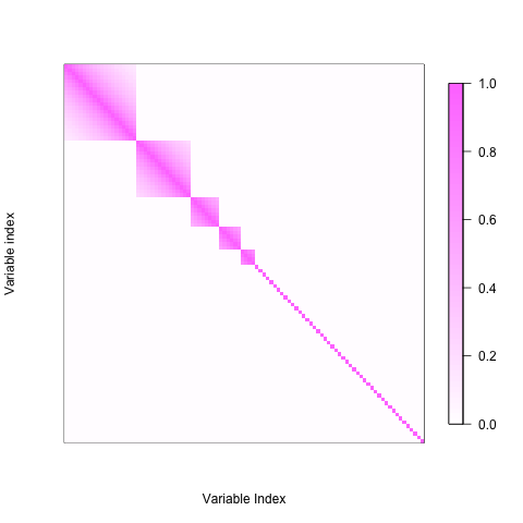
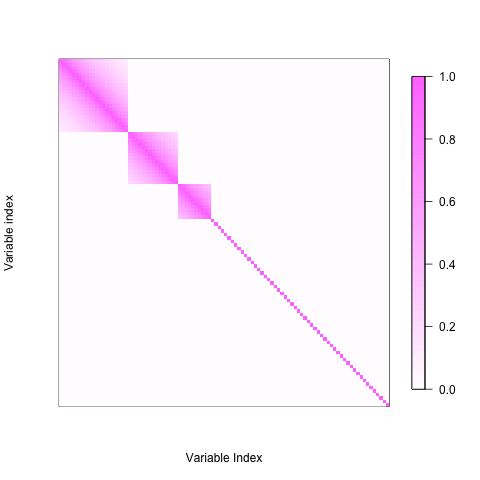
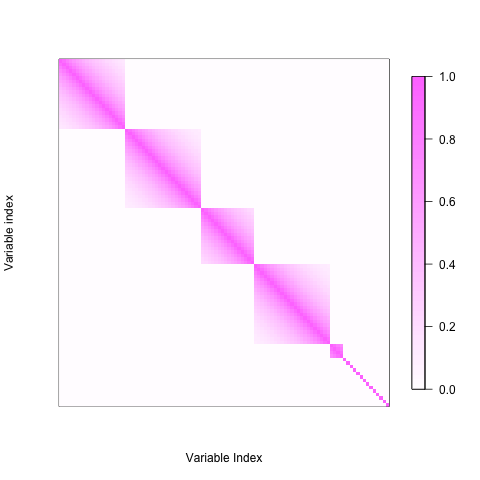
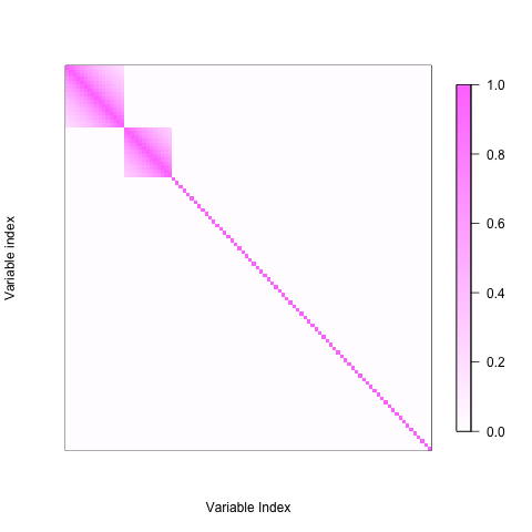
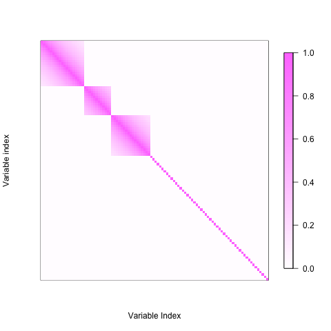
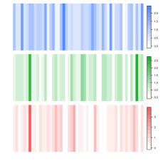
are block-diagonal matrices. The size and the number of blocks are randomly chosen. We consider the following structure of dependence in the blocks: each block is a Toeplitz matrix with an auto-correlation parameter set to 0.9. In Figure 1, we represent images of a sample of covariance matrices for . Note that the number and the size of blocks differ between clusters.
To characterize the difficulty of a simulation setting, we consider the definition of SNR (Signal-to-Noise Ratio) proposed by Devijver, (2015) as a multivariate counterpart of standard SNR when parameters are matrices. We define by the signal-to-noise ratio restricted to cluster defined as:
The SNR of the whole simulation plan across all clusters is defined by:
For example, in the simulation setting described hereafter, we observe the following value on a given sample SNR, SNR, SNR, SNR, SNR and SNR.
We consider two distinct sample sizes:
-
(A)
equals to the true number of parameters (block diagonal structure for ).
-
(B)
In order to assess the sensibility of the compared methods to the number of observations, we also consider a situation with which is 10 times lower than (A).
The predictive performances of the proposed method are compared to two versions of the model defined in Equations (6) and (7) as follows:
-
•
GLLiM: We denote by GLLiM the version of the model proposed by Deleforge et al., 2015b under heterotropic assumption on the matrices . In this paper, the authors suppose that each matrix is diagonal. This very simple version of the model minimizes the number of parameters to estimate and does not involve hyper parameters to estimate but it relies on a strong assumption on covariance structure. As proposed by Deleforge et al., 2015b , the number of affine components is determined by minimizing BIC criterion.
-
•
GLLiM-: The authors of Deleforge et al., 2015b also propose an hybrid version of GLLiM, by completing the observed response with latent factors. They estimate not only diagonal matrices but also the loadings associated to these hidden variables, within each clusters. The latent factors can be seen as extra unobserved latent responses in the inverse regression, which leads to increase the rank of matrix . The number of factors, namely the rank of the loadings matrices has to be determined. The authors propose to use the BIC criterion to estimate both hyper parameters: number of hidden factors and number of affine components . We denote this method by GLLiM- in the current paper.
3.1.2. Assessment of prediction accuracy
We assess the prediction accuracy of a given prediction procedure by computing the Root Mean Square Error (RMSE). For if denotes the -th observed response corresponding to a testing observation , if denotes the -th response predicted by a given method from the testing profile , then RMSE for response is computed as follows:
| (11) |
where is the number of testing profiles. RMSE is a common scale-dependent measure, which is on the same scale as the response. Due to its Savage-Bergman form Savage, (1971), the associated scoring function is strictly consistent with the mean functional relative to the class of the probability distributions on whose second moment is finite. As discussed in Gneiting, (2011), this criterion is relevant for models whose prediction is based on an expectation, as for BLLiM, as well as the other methods we compare BLLiM with.
In this simulation setting, performances of each method are assessed 100 times: 100 independent learning datasets are generated to train the several compared models and the respective RMSE are computed through a testing dataset, generated independently from training data and consisting in observations. Empirical means and standard deviations of RMSE are therefore computed over those 100 repetitions.
3.1.3. Results
Results are presented in Table 1. Unsurprisingly, BLLiM performs better than GLLiM as GLLiM ignores the dependence among covariates conditionally on the variable to predict. It illustrates that accounting for dependence in this inverse regression framework is crucial to achieve good prediction rates when covariates are correlated. BLLiM performs slightly better than GLLiM-, which demonstrates that our block diagonal approach can achieve good prediction rates compared to GLLiM-, while providing a more interpretable model from a biological point of view, as illustrated in Section 4. Finally, the number of observations does not seem to have a strong impact on the prediction results of the proposed method. It is interesting because it suggests that the block diagonal structure is correctly estimated, even when the number of observations is smaller than the true number of parameters to estimate, which is often the case on real data. The impact of sample size does not seem to have a strong impact on predictive performance of GLLiM, which is consistent as this model depends on a small number of parameters regarding to the two other compared methods. Moreover, the number of observations has a stronger impact on predictive performance of GLLiM-Lw but this method remains competitive in prediction.
| Number of observations | ||||
|---|---|---|---|---|
| Method | Response 1 | Response 2 | Response 1 | Response 2 |
| BLLiM | 0.078 (0.020) | 0.079 (0.015) | 0.105 (0.052) | 0.116 (0.098) |
| GLLiM | 0.169 (0.062) | 0.152 (0.022) | 0.183 (0.059) | 0.168 (0.023) |
| GLLiM- | 0.072 (0.002) | 0.083 (0.002) | 0.136 (0.036) | 0.147 (0.038) |
3.2. Prediction of high-dimensional simulated manifolds
In order to compare our procedure with other nonlinear regression methods of the literature, we consider some nonlinear link functions, relying on latent variables, with several covariance structures. It is built on the simulation plan of Deleforge et al., 2015b .
3.2.1. Simulation of high-dimensional manifolds
We generate several datasets with covariates and a response which is partially observed, where is the observed part and is the latent part of the response. The covariates are related to the response through the following inverse model:
where the different nonlinear functions considered in this paper are described hereafter and is a Gaussian noise with several dependence structures detailed hereafter. These synthetic data are generated according to an inverse approach but the goal is to retrieve the observed part of the response from the covariates .
The phenotype response is multidimensional and partially observed: the quantitative trait is observed but and are two unobserved quantitative traits. Genes are simulated from , and , but we only seek to predict the observed quantitative trait . However, the link between and also depends on the unobserved quantitative traits and , which increases the complexity of the prediction problem on purpose.
We consider three different forms of inverse regression functions denoted by , and such as each component is, for ,
The vector of covariates has dimension and is generated dimension by dimension through one of each nonlinear function described above.
The observed response is uniformly sampled in and the hidden responses are uniformly sampled in . For each of the three functions, 100 training and 100 testing datasets are generated with observations. For each of the 100 runs, a set of parameters is uniformly sampled such as , , , and and used to generate the profiles of covariates. This means that the difficulty of the problem differs at each run. This simulation plan allows to cover a large range of situations. Moreover, adding unobserved responses is interesting to study the sensibility of BLLiM to the presence of partially observed response.
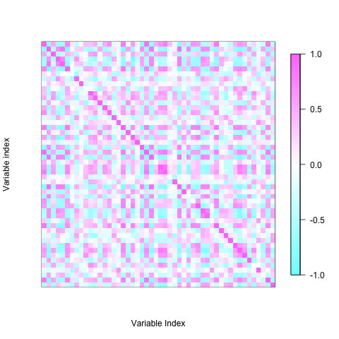
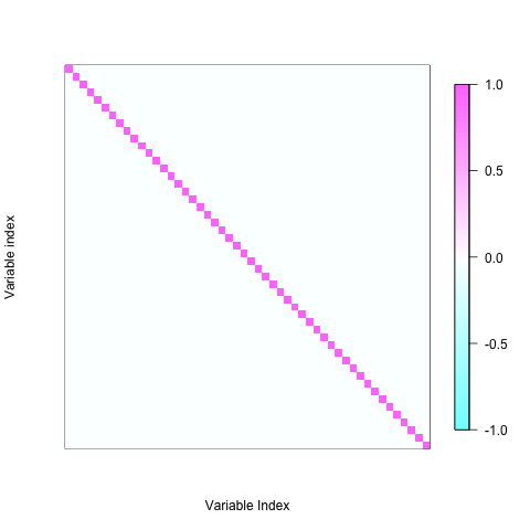
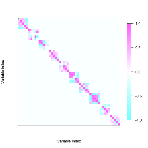
We consider several dependence structures for described hereafter and displayed on Figure 2:
-
•
Factor structure: each is decomposed as where is a -diagonal matrix and is a matrix, with . For each run of the simulations, in this sparse and low rank decomposition, and are randomly generated such as , which mimics general strong dependence patterns (see for example Friguet et al., (2009); Leek and Storey, (2007, 2008); Perthame et al., 2016b for more details). The matrix is normalized to be a correlation matrix. This design is favorable to GLLiM- as latent factors are underlying in the structure of .
-
•
Toeplitz structure: each is a Toeplitz matrix whose term indexed by is . This design is also a strong temporal dependence pattern of an autoregressive process. This design is not favorable for both BLLiM and GLLiM-Lw.
-
•
Independence structure: each is set to the identity.
-
•
Blocks structure: contains 10 blocks of 5 variables. Factor decomposition () holds on in each block with a strong dependence structure. Each block is independent from the others and independently generated among clusters.
The prediction accuracy of those methods is assessed by the RMSE described in (11).

3.2.2. Compared methods
In this simulation study, we propose to compare our method to model-based and non model-based prediction methods of the literature. The following methods are compared:
-
•
Model-based approaches
-
–
BLLiM: the proposed method described in Section 2.2, where both and the block diagonal structures of are selected by the slope heuristic;
-
–
GLLiM: standard version of GLLiM with heteroscedastic noise ( are diagonal). The number of affine components is selected by minimizing BIC criterion, as proposed in Deleforge et al., 2015b ;
-
–
GLLiM-Lw: hybrid version of GLLiM, in which latent factors can be added to complete the response when it is partially observed, both are selected by minimizing BIC criterion, as proposed in Deleforge et al., 2015b ;
-
–
MARS: multiple adaptive regression splines proposed by Friedman, (1991) and implemented in the mda R package;
-
–
SIR: sliced inverse regression, introduced by Li, (1991), followed by polynomial regression with polynomial function of order 3. Results are presented for 2 directions as it is the number of slices that provides the best results. SIR directions are extracted using the dr R package;
-
–
nonlinear PLS proposed by Wold et al., (1989) and implemented in the ppls R package. Parameters are tuned by cross-validation (CV) as proposed in the package;
-
–
K-plane proposed by Manwani and Sastry, (2015). This method is based on an approach similar to GLLiM and estimation is based on EM-algorithm. We present the results for as this number provides the best results for this method. A Matlab code implementing the method is available on https://services.math.duke.edu/yiwang/KMapRT.htm.
-
–
-
•
Non model-based approaches
Even if these competitive methods do not provide interpretable results from a biological point of view, they are known to achieve very good prediction results so it could be interesting to compare our model-based approach in terms of prediction accuracy. Therefore, our procedure is compared to the following methods:
3.2.3. Results
Table LABEL:TableVariete2 presents the results of the procedures described in Section 3.2.2 for the three nonlinear regression functions and for the four several covariance structures described in Section 3.2.1.
| Factor structure | Toeplitz structure | |||||
|---|---|---|---|---|---|---|
| f | g | h | f | g | h | |
| Model-based methods | ||||||
| BLLiM | 0.965 (0.333) | 1.749 (0.359) | 1.927 (0.353) | 1.097 (0.402) | 1.725 (0.487) | 2.025 (0.498) |
| GLLiM | 1.205 (0.321) | 2.201 (0.389) | 2.250 (0.371) | 1.598 (0.269) | 2.417 (0.380) | 2.495 (0.401) |
| GLLiM-Lw | 0.841 (0.314) | 1.749 (0.384) | 1.838 (0.342) | 1.049 (0.208) | 1.846 (0.346) | 1.920 (0.358) |
| MARS | 1.039 (0.209) | 1.873 (0.416) | 1.790 (0.377) | 0.796 (0.154) | 1.490 (0.375) | 1.580 (0.364) |
| SIR | 1.497 (0.584) | 1.771 (0.537) | 1.712 (0.537) | 1.282 (0.569) | 1.582 (0.615) | 1.594 (0.581) |
| nonlinear PLS | 0.763 (0.136) | 1.388 (0.286) | 1.350 (0.289) | 0.580 (0.102) | 1.116 (0.253) | 1.182 (0.266) |
| Kplane | 1.079 (0.478) | 1.446 (0.703) | 1.421 (0.636) | 0.917 (0.388) | 1.272 (0.585) | 1.308 (0.664) |
| Non model-based methods | ||||||
| randomForest | 1.124 (0.196) | 1.595 (0.263) | 1.644 (0.260) | 1.081 (0.155) | 1.541 (0.246) | 1.629 (0.250) |
| SVM | 1.006 (0.135) | 1.404 (0.200) | 1.449 (0.186) | 0.925 (0.116) | 1.334 (0.192) | 1.392 (0.199) |
| RVM | 1.366 (0.229) | 2.394 (0.539) | 2.535 (0.583) | 0.997 (0.174) | 2.004 (0.552) | 1.949 (0.509) |
| Independence structure | Blocks structure | |||||
| f | g | h | f | g | h | |
| Model-based methods | ||||||
| BLLiM | 0.743 (0.305) | 1.301 (0.286) | 1.556 (0.343) | 0.658 (0.273) | 1.221 (0.308) | 1.564 (0.342) |
| GLLiM | 0.710 (0.272) | 1.553 (0.248) | 1.841 (0.324) | 0.777 (0.254) | 1.566 (0.301) | 1.952 (0.346) |
| GLLiM-Lw | 0.640 (0.170) | 1.463 (0.287) | 1.603 (0.297) | 0.710 (0.176) | 1.451 (0.326) | 1.704 (0.304) |
| MARS | 1.620 (0.279) | 2.367 (0.401) | 2.439 (0.434) | 1.360 (0.256) | 2.115 (0.404) | 2.295 (0.406) |
| SIR | 1.888 (0.571) | 2.339 (0.417) | 2.342 (0.408) | 1.731 (0.642) | 2.044 (0.504) | 2.113 (0.442) |
| nonlinear PLS | 1.205 (0.172) | 1.878 (0.242) | 1.898 (0.257) | 1.061 (0.183) | 1.732 (0.331) | 1.814 (0.293) |
| Kplane | 1.412 (0.579) | 1.714 (0.618) | 1.739 (0.659) | 1.262 (0.552) | 1.601 (0.693) | 1.624 (0.668) |
| Non model-based methods | ||||||
| randomForest | 1.205 (0.219) | 1.704 (0.221) | 1.798 (0.245) | 1.234 (0.224) | 1.681 (0.290) | 1.833 (0.237) |
| SVM | 1.154 (0.158) | 1.612 (0.159) | 1.684 (0.188) | 1.122 (0.164) | 1.545 (0.210) | 1.658 (0.198) |
| RVM | 2.413 (0.378) | 3.694 (0.592) | 3.668 (0.652) | 2.011 (0.397) | 3.229 (0.708) | 3.252 (0.612) |
Note that the regression functions and are harder to estimate than , due to the hidden variables playing a nonlinear role. This design of partially observed response is difficult to catch. In contrast, is a linear function in hidden variables, and the design of partially observed response is easier to catch for every method.
As expected, BLLiM outperforms other methods on data simulated with a block diagonal residual covariance matrix. Indeed, BLLiM is able to identify the underlying block diagonal structure of correlation matrices in order to improve prediction rates.
It is interesting to note that BLLiM performs well on the independent structure, which suggests that BLLiM does not impose non-zero correlation structure and detect small blocks, when predictors are independent. BLLiM outperforms other methods for the regression functions and .
On data simulated with the factor structure, BLLiM is competitive with other methods. Nonlinear PLS and SVM perform better, but BLLiM achieves good prediction accuracy. For example, it performs as well as GLLiM-Lw, which is designed to catch such correlation matrices. It is interesting to notice that the block structure succeed to adapt itself to model the factor structure.
Remark that the Toeplitz design is harder to catch by BLLiM procedure. Performances are outperformed by nonlinear PLS, Kplane, and SVM.
Finally, remark that MARS and the nonlinear PLS achieve similar prediction results than BLLiM, or even better in some cases which suggests that it is challenging to improve their prediction performance. However, the main advantage of BLLiM is that it provides an interpretable model, which will be highlighted in Section 4.
4. Application on the prediction of olfactory behaviour from transcriptomic data
In this section, the performances and the interpretability of our model are illustrated on a study that aims at understanding the biological variation of olfactory behaviour in drosophila, an animal model widely used in genetics Roberts, (2006). To this end, we use the ressources available from the Drosophila Melanogaster Reference Panel Project (DGRP) Mackay et al., (2012), a community resource developed to analyze population genomics and quantitative traits.
Understanding natural variation in olfactory behaviour can help to understand survival and reproduction. Swarup et al., (2013) have measured a response index to exposure of benzaldehyde for 163 inbred drosophila lines from the DGRP for males and females. A response index of 1 corresponds to a maximal aversive response to the benzaldehyde source whereas a response index of 0 means that all flies remain close to source. To understand natural variation in olfactory behaviour, Swarup et al., (2013) have performed three complementary genome-wide association studies. In another article, Huang et al., (2015) have described how the variation in RNA level is a link between the variation at the DNA level and the phenotype. We have downloaded the response index to benzaldehyde and the transcriptomic data for each inbred drosophila lines (male and female) from the following link http://dgrp2.gnets.ncsu.edu/data.html. In Huang et al., (2015), measurement of genes expression have been performed for 18140 genes and 205 inbred drosophila lines, for males and females. Two replicates are available for the transcriptomic dataset, only one replicate was available for the response index to benzaldehyde, for each inbred line. We took the mean value of the two replicates for the transcriptomic dataset. To preselect genes, we first retained the top highest variable genes. For each remaining genes, we computed a model independent measure of variable importance using a non parametric method described in Kuhn, (2008), Section 9: a LOESS smoother is fit between the response index and each gene expression. For an univariate response, a coefficient of determination is computed as follows:
where is the observed response of subject , is the corresponding prediction by a LOESS regression with only predictor and is the mean of responses . The collection of coefficients of determination is used as a relative measure of variable importance of each gene to predict the olfactory behaviour. We kept the top 50 genes with the highest measure of importance. The final dataset consists in one quantitative trait variable () and transcriptomic data for 50 genes (), collected on the same inbred drosophila (). The dataset also contains one variable: the sex of each subject, male or female. This variable is not included to perform prediction and is used for downstream biological interpretation of the analysis. We performed prediction using BLLiM procedure on this dataset. The range of clusters has been tested. Increasing the number of clusters leads to empty clusters. To select the number of clusters, we have used BIC instead of the slope heuristic because there are not enough points to calibrate the coefficient in the slope heuristic.
In the following subsection, our model is compared by cross-validation with other prediction strategies to demonstrate the good predictive performance of our method. In the final section, the clustering of individuals performed to catch the nonlinear relationship between the quantitative trait to predict and the transcriptomic data is analyzed. Subsequently, we explore and compare the gene regulatory networks inferred in each cluster of individuals.
4.1. Assessment of prediction accuracy
In this section, our prediction strategy is compared to other prediction strategies by a 10-fold cross validation procedure. Predictive performances of the methods are measured by the RMSE, defined in (11). More precisely, we compute the RMSE for each run of the 10-fold cross validation procedure, and we repeat it 50 times to consider statistics of this criterion. Each method is therefore assessed 500 times. The results are presented in Table 3. Our procedure achieves challenging prediction performances, similar to nonlinear PLS and non model-based methods. Non model-based methods are known to perform well in difficult setting and real data but the downstream model interpretation is not clear. In nonlinear PLS, the nonlinear relationship between latent variables is not as easy to interpret as latent factors do not represent any biological entities. Moreover, we outperform the prediction error of MARS, SIR and K-plane. For example, K-plane has very good performances on simulated dataset, as described in Table LABEL:TableVariete2, but perform poorly on this real dataset. Note that, for the K-plane prediction, the authors do not propose a criterion to choose the number of components. We choose the number of components that minimizes the prediction error on testing data, which is rather optimistic as testing data should not be used to tune hyper parameters.
| Method | RMSE (sd) | ||
|---|---|---|---|
| Model-based methods | |||
| BLLiM | 0.0798 (0.002) | ||
| GLLiM | 0.0970 (0.003) | ||
| GLLiM- | 0.0850 (0.001) | ||
| MARS | 0.0924 (0.003) | ||
| SIR | 0.0836 (0.001) | ||
| nonlinear PLS | 0.0748 (0.001) | ||
| K-plane | 0.1039 (0.004) | ||
| Non model-based methods | |||
| Random Forest | 0.0764 (4e-4) | ||
| SVM - Gaussian kernel | 0.0764 (5e-4) | ||
| RVM - Linear kernel | 0.0742 (0.001) |
4.2. Interpretation of BLLiM model
To approximate the nonlinear function which relates the phenotypic variable to the expression data, BLLiM separates drosophila into 3 clusters of sizes 163, 106 and 57. In fact, cluster 1 corresponds to male drosophila (in red in the plots), whereas clusters 2 and 3 correspond to female drosophila (in green and blue in the plots). The correspondence of these inferred clusters and the external information (sex) demonstrates the ability of our model to take into account hidden observations stratification: even though the sex information is not included into the model, the proposed method is able to retrieve this information from the data.
The response index to benzaldehyde in each cluster of drosophila is represented in Figure 3 (Left). We notice no significant differences between the response index among the clusters. Indeed, the clustering is based on the relation between response and covariates, and not on the value of the response. In contrast, the values taken by coefficients in the linear regression are highly different between clusters, as illustrated in Figure 3 (Right). These differences demonstrate the necessity of taking nonlinearity into account. The genes contributing the most to the prediction of response index to benzaldehyde differ between clusters.
In a similar way, the modules of the inferred gene regulatory network are not similar among clusters. For cluster 1 (males), 3 modules of size 19, 5 and 2 are detected. For cluster 2, 5 modules of size 12, 7, 5, 2 and 2 are detected. For cluster 3, 8 modules of size 9, 8, 4, 3, 3, 2, 2, and 2 are detected. The sizes of the modules are smaller than the genes we consider. The corresponding modules are represented in Figure 4. We obtain a sparse representation of the network underlying the phenotype transcriptome relationship for each cluster of individuals. Remark that isolated genes are not displayed in Figure 4.


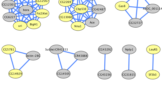
A merged version of the 3 different networks presented in Figure 4 is presented in Figure 5. A core set of 17 genes is detected in a network in every cluster. These genes are highlighted in yellow in Figures 4 and 5. Few genes belong to exactly two clusters: 2 genes between clusters 1 (red) and 2 (green), 6 genes between clusters 2 (green) and 3 (blue), and 3 genes between clusters 1 (red) and 3 (blue), and some are detected only in one cluster.
Among the list of 17 genes in modules for each cluster of individuals, we notice that genes Sf3b3 and LeuRS are always interconnected, for cluster 1 (red), cluster 2 (green) and cluster 3 (blue). Genes Sf3b3 and LeuRS are known to be implicated in neurogenesis Neumüller et al., (2011), and olfactory behaviour is known to be linked with neurogenesis cellular processes. This observation is consistent with the GWA studies performed in Swarup et al., (2013). Similarly, genes Cadps and Cpb53E are always interconnected, in cluster 1 (red), cluster 2 (green) and cluster 3 (blue). This results is not surprising either, given that agressive behaviour has an olfactory component and that Cadps and Cpb53E are known to be associated with neurotransmitter secretion Lloyd et al., (2000) and negative regulation of response to wounding Wishart et al., (2012), respectively. Gene Hk, found in the inferred network for cluster 1 (males), is known to be implicated in flight behaviour Homyk and Sheppard, (1977). Conversely, gene Nplp1, is known to be implicated in neuropeptide signaling pathway Baggerman et al., (2002), is only found in modules for cluster 3 (cluster of 57 females). Genes pim (in modules for all clusters) and Hsp68 (in modules for cluster 1 only) are also known to be implicated in neurogenesis Neumüller et al., (2011). Among the 17 genes in modules for each cluster of individuals, we also notice gene Gas8, known to be implicated in process involved in the controlled movement of a flagellated sperm cell, gene Fs (2)Ket, known to be linked with the construction of a chorion-containing eggshell Schupbach and Wieschaus, (1991), and gene grp, known to be implicated in female meiosis chromosome segregation Dobie et al., (2001). These genes are linked with reproduction, which is known to have an olfactory component. Several genes identified in modules for all clusters, such as CG13060 and CG2269 have not been identified before as linked to the variation in olfactory behaviour in adult drosophila and can be investigated in further studies. These results, based on the phenotype-transcriptome relationship study, may complete classical GWA studies and help to improve the understanding of the natural variation of olfactory behaviour.
The code to reproduce the complete real data analysis has been provided as supplementary materials.
5. Discussion
In this paper, an interpretable statistical framework is proposed to perform non linear prediction from transcriptomic data. Our prediction method performs well on simulated and real data and is competitive with other prediction models, including machine learning techniques. Unlike other methods, the proposed model is fully parametric and interpretable: the nonlinear relationship between the phenotypical variables to predict and the transcriptome data is modeled by locally linear regressions, clusters of individuals are encoded by hidden variables associated with a mixture of linear regressions model and the relationship between genes is encoded by a block structure in the conditional covariance matrices of the model.
In this paper, our method has been used on a real dataset with 50 covariates. Considering the number of parameters with respect to the number of observations, the limits of BLLiM would be reached if the number of variables grows to thousands while the number of observations remains around hundreds, which is an usual design in genomics studies. A standard idea in this context of unbalanced design is to regularize the estimation of regression coefficients in order to reduce dimension. Introducing a sparse structure in the regression coefficients of the inverse regression, namely the collection of matrices would be particularly relevant in the BLLiM framework. It is interesting to notice that the estimated matrices displayed on Figure 3 (Right) exhibit a sparse structure which would be a valuable information to account for in the model.
Besides, the proposed method is based on a mixture of linear regressions, which allows to estimate gene regulatory networks within each cluster of the mixture. Both on biological and statistical point of view, it could be valuable to include in the model a regulatory network common to all clusters, and cluster-specific networks, in the manner of the joint graphical lasso Danaher et al., (2014). Some genes would therefore be shared among clusters of individuals : some modules would be shared across different clusters of individuals (functional modules), some modules would be specific for each cluster (disease modules).
In this paper, the BLiMM method is applied on transcriptomic data to study the olfactory behaviour of drosophila. As going from the genome level to the transcriptome level helps to gain deeper insights into complex biological diseases such as cancers Rhodes and Chinnaiyan, (2005), an application of our model on cancer data would be of particular interest in the context of network medicine, as described by Barabási et al., (2011): modules detected for each set of individuals may correspond to functional modules or disease modules. The performance of the method is demonstrated on transcriptomic data but other "omics" data can be used, such metabolomic data or proteomic data. Our model would also be useful in the context of trans"omics" data Yugi et al., (2016), combining data from multiple "omics" layers to understand deeper biological processes.
Finally, our prediction framework can be used to perform prediction on any dataset with heterogeneous observations and hidden graph-structured interactions between covariates. This framework is of interest beyond molecular biology, and can be useful in other fields (neurology, ecology or sociology).
Acknowledgements
Emilie Devijver is supported by the Interuniversity Attraction Poles Programme (IAP-network P7/06), Belgian Science Policy Office, whose funding is gratefully acknowledged. We thank Jordi Estellé (INRA, Jouy-en-Josas, France) for suggesting the Drosophila Melanogaster Genetic Reference Panel as a ressource for real data analysis.
References
- Arlot and Massart, (2009) Arlot, S. and Massart, P. (2009). Data-driven calibration of penalties for least-squares regression. Journal of Machine Learning Research, 10:245–279.
- Arumugam and Scott, (2004) Arumugam, M. and Scott, S. (2004). Emprr: A high-dimensional em-based piecewise regression algorithm. In Proceedings of International Conference on Machine Learning and Applications, pages 264–271.
- Baggerman et al., (2002) Baggerman, G., Cerstiaens, A., De Loof, A., and Schoofs, L. (2002). Peptidomics of the larval Drosophila melanogaster central nervous system. Journal of Biological Chemistry, 277(43):40368–40374.
- Barabási and Albert, (1999) Barabási, A. L. and Albert, R. (1999). Emergence of scaling in random network. Science, 286:509–512.
- Barabási et al., (2011) Barabási, A. L., Gulbahce, N., and Loscalzo, J. (2011). Network medicine: a network-based approach to human disease. Nature Reviews Geneticss, 12(1):56–68.
- Barabási and Oltvai, (2004) Barabási, A. L. and Oltvai, Z. N. (2004). Network Biology: Understanding the Cell’s Functional Organization. Nature Reviews Genetics, 5:101–113.
- Baraud et al., (2009) Baraud, Y., Giraud, C., and Huet, S. (2009). Gaussian model selection with an unknown variance. The Annals of Statistics, 37(2):630–672.
- Baudry et al., (2012) Baudry, J.-P., Maugis, C., and Michel, B. (2012). Slope heuristics: overview and implementation. Statistics and Computing, 22(2):455–470.
- Birgé and Massart, (2001) Birgé, L. and Massart, P. (2001). Gaussian model selection. Journal of the European Mathematical Society, 3(3):203–268.
- Bouveyron et al., (2015) Bouveyron, C., Côme, E., and Jacques, J. (2015). The discriminative functional mixture model for a comparative analysis of bike sharing systems. The Annals of Applied Statistics, 9(4):1726–1760.
- Breiman, (2001) Breiman, L. (2001). Random forests. Machine Learning, 45(1):5–32.
- Butte et al., (2000) Butte, A. J., Tamayo, P., Slonim, D., Golub, T. R., and Kohane, I. S. (2000). Discovering functional relationships between RNA expression and chemotherapeutic susceptibility using relevance networks. Proceedings of the National Academy of Sciences, 97(22):12182–12186.
- Candès et al., (2009) Candès, E. J., Li, X., Ma, Y., and Wright, J. (2009). Robust principal component analysis? Journal of ACM, 58(1):1–37.
- Chandrasekaran et al., (2011) Chandrasekaran, V., Sanghavi, S., Parrilo, P., and Willsky, A. (2011). Rank-sparsity incoherence for matrix decomposition. SIAM Journal on Optimization, 21(2):572–596.
- Christmas et al., (2005) Christmas, R., Avila-Campillo, I., Bolouri, H., Schwikowski, B., Anderson, M., Kelley, R., Landys, N., Workman, C., Ideker, T., Cerami, E., Sheridan, R., Bader, G. D., and Sander, C. (2005). Cytoscape: a software environment for integrated models of biomolecular interaction networks. American Association for Cancer Research Education Book, (Karp 2001):12–16.
- Chuang et al., (2007) Chuang, H. Y., Lee, E., Liu, Y. T., Lee, D., and Ideker, T. (2007). Network-based classification of breast cancer metastasis. Molecular System Biology, 3(140):140.
- Danaher et al., (2014) Danaher, P., Wang, P., and Witten, D. M. (2014). The joint graphical lasso for inverse covariance estimation across multiple classes. Journal of the Royal Statistical Society: Series B (Statistical Methodology), 76(2):373–397.
- Datta, (2001) Datta, S. (2001). Exploring relationships in gene expressions: a partial least squares approach. Gene Expression, 9(6):249–255.
- de la Fuente, (2010) de la Fuente, A. (2010). From ’differential expression’ to ’differential networking’ - identification of dysfunctional regulatory networks in diseases. Trends in Genetics, 26(7):326–333.
- (20) Deleforge, A., Forbes, F., Ba, S., and Horaud, R. (2015a). Hyper-spectral image analysis with partially-latent regression and spatial markov dependencies. IEEE journal of selected topics in signal processing, 9(6):1037–1048.
- (21) Deleforge, A., Forbes, F., and Horaud, R. (2015b). High-dimensional regression with gaussian mixtures and partially-latent response variables. Statistics and Computing, 25(5):893–911.
- Dempster et al., (1977) Dempster, A., Laird, N. M., and Rubin, D. B. (1977). Maximum likelihood from incomplete data via the EM algorithm. Journal of the Royal Statistical Society. Series B, Vol. 39(1):1–38.
- Devijver, (2015) Devijver, E. (2015). Finite mixture regression: a sparse variable selection by model selection for clustering. Electronic Journal of Statistics, 9:2642–2674.
- Devijver, (2016) Devijver, E. (2016). Model-based clustering for high-dimensional data. Application to functional data. Advances in Data Analysis and Classification, in press.
- Devijver and Gallopin, (2017) Devijver, E. and Gallopin, M. (2017). Block-diagonal covariance selection for high-dimensional gaussian graphical models. Journal of the American Statistical Association, in press.
- Dobie et al., (2001) Dobie, K. W., Kennedy, C. D., Velasco, V. M., McGrath, T. L., Weko, J., Patterson, R. W., and Karpen, G. H. (2001). Identification of chromosome inheritance modifiers in Drosophila melanogaster. Genetics, 157(4):1623–1637.
- Dong et al., (2015) Dong, Y., Yu, Z., and Zhu, L. (2015). Robust inverse regression for dimension reduction. Journal of Multivariate Analysis, 134:71–81.
- Eisen et al., (1998) Eisen, M. B., Spellman, P. T., Brown, P. O., and Botstein, D. (1998). Cluster analysis and display of genome-wide expression patterns. Proceedings of the National Academy of Sciences, 95(25):14863–8.
- Friedman, (1991) Friedman, J. (1991). Multivariate adaptive regression splines (with discussion). The Annals of Statistics, 19(1):1–141.
- Friedman et al., (2008) Friedman, J., Hastie, T., and Tibshirani, R. (2008). Sparse inverse covariance estimation with the graphical lasso. Biostatistics, 9(3):432–441.
- Friguet et al., (2009) Friguet, C., Kloareg, M., and Causeur, D. (2009). A factor model approach to multiple testing under dependence. Journal of the American Statistical Association, 104:488:1406–1415.
- Fu, (2013) Fu, Y. (2013). Complex networks and simple models in biology. Journal of the Royal Society, Interface, 2(5):419–30.
- Gneiting, (2011) Gneiting, T. (2011). Making and Evaluating Point Forecasts. Journal of the American Statistical Association, 106:494:746–762.
- Golub, (1999) Golub, T. R. (1999). Molecular classification of cancer: class discovery and class prediction by gene expression monitoring. Science, 286(5439):531–537.
- Hastie et al., (2010) Hastie, T., Tibshirani, R., and Friedman, J. (2010). The elements of statistical learning. Springer.
- Homyk and Sheppard, (1977) Homyk, T. and Sheppard, D. E. (1977). Behavioral mutants of Drosophila melanogaster. Genetics, 87:95–104.
- Huang et al., (2015) Huang, W., Carbone, M. A., Magwire, M. M., Peiffer, J. A., Lyman, R. F., Stone, E. A., Anholt, R. R. H., and Mackay, T. F. C. (2015). Genetic basis of transcriptome diversity in Drosophila melanogaster. Proceedings of the National Academy of Sciences, 112(44):E6010–9.
- Jacob et al., (2012) Jacob, L., Neuvial, P., and Dudoit, S. (2012). More power via graph-structured tests for differential expression of gene networks. The Annals of Applied Statistics, 6(2):561–600.
- Kraemer et al., (2008) Kraemer, N., Boulsteix, A.-L., and Tutz, G. (2008). Penalized partial least squares with applications to B-spline transformations and functional data. Chemometrics and ntelligent Laboratory Systems, 94:60–69.
- Kuhn, (2008) Kuhn, M. (2008). Building Predictive Models in R Using the caret Package. Journal Of Statistical Software, 28(5):1–26.
- Le Cao et al., (2008) Le Cao, K.-A., Rossow, D., Robert-Granié, C., and Besse, P. (2008). A Sparse PLS for Variable Selection when Integrating Omics data. Statistical Applications in Genetics and Molecular Biology, 7(1):pp. 35.
- Leek and Storey, (2007) Leek, J. T. and Storey, J. (2007). Capturing heterogeneity in gene expression studies by surrogate variable analysis. PLoS Genetics, 3(9):e161.
- Leek and Storey, (2008) Leek, J. T. and Storey, J. (2008). A general framework for multiple testing dependence. Proceedings of the National Academy of Sciences, 105:18718–18723.
- Letham et al., (2015) Letham, B., Rudin, C., McCormick, T. H., and Madigan, D. (2015). Interpretable classifiers using rules and bayesian analysis: Building a better stroke prediction model. The Annals of Applied Statistics, 9(3):1350–1371.
- Li, (1991) Li, K. (1991). Sliced inverse regression for dimension reduction. Journal of the American Statistical Association, 86(414):316–327.
- Lloyd et al., (2000) Lloyd, T. E., Verstreken, P., Ostrin, E. J., Phillippi, A., Lichtarge, O., and Bellen, H. J. (2000). A genome-wide search for synaptic vesicle cycle proteins in Drosophila. Neuron, 26(1):45–50.
- Mach et al., (2013) Mach, N., Gao, Y., Lemonnier, G., Lecardonnel, J., Oswald, I. P., Estellé, J., and Rogel-Gaillard, C. (2013). The peripheral blood transcriptome reflects variations in immunity traits in swine: towards the identification of biomarkers. BMC genomics, 14:894.
- Mackay et al., (2012) Mackay, T. F. C., Richards, S., Stone, E. a., Barbadilla, A., Ayroles, J. F., Zhu, D., Casillas, S., Han, Y., Magwire, M. M., Cridland, J. M., Richardson, M. F., Anholt, R. R. H., Barrón, M., Bess, C., Blankenburg, K. P., Carbone, M. A., Castellano, D., Chaboub, L., Duncan, L., Harris, Z., Javaid, M., Jayaseelan, J. C., Jhangiani, S. N., Jordan, K. W., Lara, F., Lawrence, F., Lee, S. L., Librado, P., Linheiro, R. S., Lyman, R. F., Mackey, A. J., Munidasa, M., Muzny, D. M., Nazareth, L., Newsham, I., Perales, L., Pu, L.-L., Qu, C., Ràmia, M., Reid, J. G., Rollmann, S. M., Rozas, J., Saada, N., Turlapati, L., Worley, K. C., Wu, Y.-Q., Yamamoto, A., Zhu, Y., Bergman, C. M., Thornton, K. R., Mittelman, D., and Gibbs, R. a. (2012). The Drosophila melanogaster Genetic Reference Panel. Nature, 482(7384):173–8.
- Manwani and Sastry, (2015) Manwani, N. and Sastry, P. (2015). K-plane regression. Information Sciences, 292:39 – 56.
- Neumüller et al., (2011) Neumüller, R. A., Richter, C., Fischer, A., Novatchkova, M., Neumüller, K. G., and Knoblich, J. A. (2011). Genome-Wide Analysis of Self-Renewal in Drosophila Neural Stem Cells by Transgenic RNAi. Cell Stem Cell, 8(5):580–593.
- Nguyen and Rocke, (2002) Nguyen, D. V. and Rocke, D. M. (2002). Tumor classification by partial least squares using microarray gene expression data. Bioinformatics, 18(1):39–50.
- (52) Perthame, E., Forbes, F., and Deleforge, A. (2016a). Inverse regression approach to robust non-linear high-to-low dimensional mapping. preprint hal-01347455.
- (53) Perthame, E., Friguet, C., and Causeur, D. (2016b). Stability of feature selection in classification issues for high-dimensional correlated data. Statistics and Computing, 26(4):783–796.
- Rhodes and Chinnaiyan, (2005) Rhodes, D. R. and Chinnaiyan, A. M. (2005). Integrative analysis of the cancer transcriptome. Nature Genetics, 37 Suppl:0–7.
- Roberts, (2006) Roberts, D. B. (2006). Drosophila melanogaster: the model organism. Entomologia Experimentalis et Applicata, 121(2):93–103.
- Savage, (1971) Savage, L. J. (1971). Elicitation of personal probabilities and expectations. Journal of the American Statistical Association, 66(336):783–801.
- Schupbach and Wieschaus, (1991) Schupbach, T. and Wieschaus, E. (1991). Female sterile mutations on the second chromosome of Drosophila melanogaster. Genetics, 129:1119–1136.
- Smyth, (2004) Smyth, G. K. (2004). Linear Models and Empirical Bayes Methods for Assessing Differential Expression in Microarray Experiments Linear Models and Empirical Bayes Methods for Assessing Differential Expression in Microarray Experiments. Statistical Applications in Genetics and Molecular Biology, 3(1):1–26.
- Suzuki et al., (2014) Suzuki, S., Horinouchi, T., and Furusawa, C. (2014). Prediction of antibiotic resistance by gene expression profiles. Nature Communications, 5:5792.
- Swarup et al., (2013) Swarup, S., Huang, W., Mackay, T. F. C., and Anholt, R. R. H. (2013). Analysis of natural variation reveals neurogenetic networks for Drosophila olfactory behavior. Proceedings of the National Academy of Sciences of the United States of America, 110(3):1017–22.
- Tipping, (2001) Tipping, M. E. (2001). Sparse bayesian learning and the relevance vector machine. The Journal of Machine Learning Research, 1:211–244.
- Torres-García et al., (2009) Torres-García, W., Zhang, W., Runger, G. C., Johnson, R. H., and Meldrum, D. R. (2009). Integrative analysis of transcriptomic and proteomic data of Desulfovibrio vulgaris: A non-linear model to predict abundance of undetected proteins. Bioinformatics, 25(15):1905–1914.
- Valcárcel et al., (2014) Valcárcel, B., Ebbels, T. M. D., Kangas, A. J., Soininen, P., Elliot, P., Ala-Korpela, M., Järvelin, M.-R., and de Iorio, M. (2014). Genome metabolome integrated network analysis to uncover connections between genetic variants and complex traits: an application to obesity. Journal of the Royal Society, Interface, 11(94):20130908.
- Valcárcel et al., (2011) Valcárcel, B., Wurtz, P., al Basatena, N. K. S., Tukiainen, T., Kangas, A. J., Soininen, P., Järvelin, M.-R., Ala-Korpela, M., Ebbels, T. M., and de Iorio, M. (2011). A differential network approach to exploring differences between biological states: An application to prediabetes. PLoS ONE, 6(9).
- Vapnik, (1998) Vapnik, V. (1998). Statistical Learning Theory. Wiley, New York.
- Wishart et al., (2012) Wishart, T. M., Rooney, T. M., Lamont, D. J., Wright, A. K., Morton, A. J., Jackson, M., Freeman, M. R., and Gillingwater, T. H. (2012). Combining comparative proteomics and molecular genetics uncovers regulators of synaptic and axonal stability and degeneration in vivo. PLoS Genetics, 8(8):e1002936.
- Wold et al., (1989) Wold, S., Kettaneh-Wold, N., and Skagerberg, B. (1989). Nonlinear pls modeling. Chemometrics and Intelligent Laboratory Systems, 7:53–65.
- Wu, (2008) Wu, H. (2008). Kernel sliced inverse regression with applications to classification. Journal of Computational and Graphical Statistics, 17(3):590–610.
- Yang et al., (2011) Yang, B., Bassols, A., Saco, Y., and Pérez-Enciso, M. (2011). Association between plasma metabolites and gene expression profiles in five porcine endocrine tissues. Genetics, Selection, Evolution, 43(1):28.
- Yugi et al., (2016) Yugi, K., Kubota, H., Hatano, A., and Kuroda, S. (2016). Trans-Omics : How To Reconstruct Biochemical Networks Across Multiple ’Omic’ Layers. Trends in Biotechnology, 34(4):276–290.
- Zhong et al., (2005) Zhong, W., Zeng, P., Ma, P., Liu, J., and Zhu, Y. (2005). Rsir: regularized sliced inverse regression for motif discovery. Bioinformatics, 21(22):4169–4175.
Appendix A Appendix
This appendix contains the details of the updates of parameters estimations of our algorithm.
A.1. Details on the E-step of algorithm
Individual probabilities are updated by, for the iteration ,
These probabilities can be expressed in function of all marginals using Bayes formula.
A.2. Details on the M-step of algorithm
GMM-like estimators
, and are estimated by GMM-like estimators as in Deleforge et al., 2015b
Regression-like estimators
For , and are estimated by Regression-like estimators as in Deleforge et al., 2015b
where and are the observations reweighted by the cluster weights and are expressed in function of the observed data:
Block-diagonal covariance estimator
In GLLiM, for , is estimated as the diagonal of the residual covariance matrix of the regression of on in each cluster and weighted by the cluster weights . In this paper, we propose to replace this estimation step by a block-diagonal covariance matrix, and then is estimated by a block-diagonal estimator, as explained in Section 2.2.