Geometric Ergodicity of the multivariate COGARCH(1,1) Process

Robert Stelzer Institute of Mathematical Finance, Ulm University, Helmholzstraße 18, D-89069 Ulm, E-mail: robert.stelzer@uni-ulm.de    Johanna Vestweber Institute of Mathematical Finance, Ulm University, Helmholzstraße 18, D-89069 Ulm, E-mail: johanna.vestweber@uni-ulm.de
Abstract

For the multivariate COGARCH(1,1) volatility process we show sufficient conditions for the existence of a unique stationary distribution, for the geometric ergodicity and for the finiteness of moments of the stationary distribution by a Foster-Lyapunov drift condition approach. The test functions used are naturally related to the geometry of the cone of positive semi-definite matrices and the drift condition is shown to be satisfied if the drift term of the defining stochastic differential equation is sufficiently “negative”. We show easily applicable sufficient conditions for the needed irreducibility and aperiodicity of the volatility process living in the cone of positive semidefinite matrices, if the driving Lévy process is a compound Poisson process.

AMS Subject Classification 2010: Primary: 60J25   Secondary: 60G10, 60G51

Keywords: Feller process, Foster-Lyapunov drift condition, Harris recurrence, irreducibility, Lévy process, MUCOGARCH, multivariate stochastic volatility model

1 Introduction

General autoregressive conditionally heteroscedastic (GARCH) time series models, as introduced in [12], are of high interest for financial economics. They capture many typical features of observed financial data, the so-called stylized facts (see [37]). A continuous time extension, which captures the same stylized facts as the discrete time GARCH model, but can also be used for irregularly-spaced and high-frequency data, is the COGARCH process, see e.g. [40, 41, 15]. The use in financial modelling is studied e.g. in [42, 57, 7] and the statistical estimation in [38, 11, 47], for example. Furthermore, an asymmetric variant is proposed in [9] and an extension allowing for more flexibility in the autocovariance function in [8].

To model and understand the behavior of several interrelated time series as well as to price derivatives on several underlyings or to assess the risk of a portfolio multivariate models for financial markets are needed. The fluctuations of the volatilities and correlations over time call for employing stochastic volatility models which in a multivariate set-up means that one has to specify a latent process for the instantaneous covariance matrix. Thus, one needs to consider appropriate stochastic processes in the cone of positive semi-definite matrices. Many popular multivariate stochastic volatility models in continuous time, which in many financial applications is preferable to modelling in discrete time, are of an affine type, thus falling into the framework of [19, 51]. Popular examples include the Wishart (see e.g. [3, 17, 35]) and the Ornstein-Uhlenbeck type stochastic volatility model (see [56, 10, 36], for example). Thus the price processes have two driving sources of randomness and the tail-behavior of their volatility process is typically equivalent to the one of the driving noise (see [55, 31]). A very nice feature of GARCH models is that they have only one source of randomness and their structure ensures heavily-tailed stationary behavior even for very light tailed driving noises ([32, 5]). In discrete time one of the most general multivariate GARCH versions (see [6, 34] for an overview) is the BEKK model, defined in [27], and the multivariate COGARCH(1,1) (shortly MUCOGARCH(1,1)) process introduced and studied in [67], is the continuous time analogue, which we are investigating further in this paper.

The existence and uniqueness of a stationary solution as well as the convergence to the stationary solution is of high interest and importance. Geometric ergodicity ensures fast convergence to the stationary regime in simulations and paves the way for statistical inference. By the same argument as in [50, Proof of Theorem 4.3, Step 2] geometric ergodicity and the existence of some p𝑝p-moments of the stationary distribution provide exponential β𝛽\beta-mixing for Markov processes. This in turn can be used to show a central limit theorem for the process, see for instance [24], and so allows to prove for example asymptotic normality of estimators (see e.g. [38, 11] in the context of univariate COGARCH(1,1) processes). In a similar way [23, 22] employ the results of the present paper to analyse moment based estimators of the parameters of MUCOGARCH(1,1) processes.

In many applications involving time series (multivariate) ARMA-GARCH models (see e.g. [33, 46, 18]) turn out to be adequate and geometric ergodicity is again key to understand the asymptotic behaviour of statistical estimators. In continuous time a promising analogue currently investigated in [59] seems to be a (multivariate) CARMA process (see e.g. [16, 30, 49]) driven by a (multivariate) COGARCH process. The present paper also lays foundations for the analysis of such models.

For the univariate COGARCH process geometric ergodicity was shown by [29] and [14] discussed it for the BEKK GARCH process. In [67] for the MUCOGARCH process sufficient conditions for the existence of a stationary distribution are shown by tightness arguments, but the paper failed to establish uniqueness or convergence to the stationary distribution. In this paper we deduce under the assumption of irreducibility sufficient conditions for the uniqueness of the stationary distribution, the convergence to it with an exponential rate and some finite p𝑝p-moment of the stationary distribution of the MUCOGARCH volatility process Y𝑌Y. To show this we use the theory of Markov process, see e.g. [52, 25]. A further result of this theory is, that our volatility process is positive Harris recurrent. If the driving Lévy process is a compound Poisson process, we show easily applicable conditions ensuring irreducibility of the volatility process in the cone of positive semidefinite matrices.

Like in the discrete time BEKK case the non-linear structure of the SDE prohibits us from using well-established results for random recurrence equations like in the one-dimensional case and due to the rank one jumps establishing irreducibility is a very tricky issue. To obtain the latter [14] in discrete time used techniques from algebraic geometry (see also [13]) whereas we use a direct probabilistic approach playing the question back to the existence of a density for a Wishart distribution. However, we restrict ourselves to processes of order (1,1) while in the discrete time BEKK case general orders were considered. The reason is that on the one hand order (1,1) GARCH processes seem sufficient in most applications and on the other hand multivariate COGARCH(p,q) processes can be defined in principle ([66, Section 6.6]), but no reasonable conditions on the possible parameters are known. Already in the univariate case these conditions are quite involved (cf. [15, Section 5], [68]). On the other hand we look at the finiteness of an arbitrary p𝑝p-th moment (of the volatility process) and use drift conditions related to it, whereas [14] only looked at the first moment for the BEKK case. In contrast to [67] we avoid any vectorizations, work directly in the cone of positive semi-definite matrices and use test functions naturally in line with the geometry of the cone.

After a brief summary of some preliminaries, notations and Lévy processes, the remainder of the paper is organized as follows: In Section 3 we recall the definition of the MUCOGARCH(1,1) process and some of its properties of relevance later on. In Section 4 we present our first main result: sufficient conditions ensuring the geometric ergodicity of the volatility process Y𝑌Y. Furthermore, we compare the conditions for geometric ergodicity to previously known conditions for (first order) stationarity. Moreover, we discuss the applications of the obtained results and illustrate them by exemplary simulations. In Section 5 we establish sufficient conditions for the irreducibility and aperiodicity of Y𝑌Y needed to apply the previous results on geometric ergodicity. Section 6 first gives a brief repetition of the Markov theory we use and the proofs of our results are developed.

2 Preliminaries

Throughout we assume that all random variables and processes are defined on a given filtered probability space (Ω,,,(t)t𝒯)Ωsubscriptsubscript𝑡𝑡𝒯(\Omega,\mathcal{F},\mathbb{P},(\mathcal{F}_{t})_{t\in\mathcal{T}}) with 𝒯=𝒯\mathcal{T}=\mathbb{N} in the discrete time case and 𝒯=+𝒯superscript\mathcal{T}=\mathbb{R}^{+} in the continuous one. Moreover, in the continuous time setting we assume the usual conditions (complete, right continuous filtration) to be satisfied.

For Markov processes in discrete and continuous time we refer to [54] and respectively [26, 2]. A summary of the most relevant notions and results from Markov processes is given in Section 6.1 for the convenience of the reader.

2.1 Notation

The set of real m×n𝑚𝑛m\times n matrices is denoted by Mm,n()subscript𝑀𝑚𝑛M_{m,n}(\mathbb{R}) or only by Mn()subscript𝑀𝑛M_{n}(\mathbb{R}) if m=n𝑚𝑛m=n. For the invertible n×n𝑛𝑛n\times n matrices we write GLn()𝐺subscript𝐿𝑛GL_{n}(\mathbb{R}). The linear subspace of symmetric matrices we denote by 𝕊nsubscript𝕊𝑛\mathbb{S}_{n}, by 𝕊n+superscriptsubscript𝕊𝑛\mathbb{S}_{n}^{+} the closed cone of positive semi-definite matrices and the open cone of positive definite matrices by 𝕊n++superscriptsubscript𝕊𝑛absent\mathbb{S}_{n}^{++}. Further we denote by Insubscript𝐼𝑛I_{n} the n×n𝑛𝑛n\times n identity matrix.
We introduce the natural ordering on 𝕊nsubscript𝕊𝑛\mathbb{S}_{n} and denote it by precedes-or-equals\preceq, that is for A,B𝕊n𝐴𝐵subscript𝕊𝑛A,B\in\mathbb{S}_{n} it holds ABBA𝕊n+precedes-or-equals𝐴𝐵𝐵𝐴superscriptsubscript𝕊𝑛A\preceq B\ \Leftrightarrow\ B-A\in\mathbb{S}_{n}^{+}. The tensor (Kronecker) product of two matrices A,B𝐴𝐵A,B is written as ABtensor-product𝐴𝐵A\otimes B. vecvec\mathrm{vec} denotes the well-known vectorization operator that maps the n×n𝑛𝑛n\times n matrices to n2superscriptsuperscript𝑛2\mathbb{R}^{n^{2}} by stacking the columns of the matrices below another. The spectrum of a matrix is denoted by σ()𝜎\sigma(\cdot) and the spectral radius by ρ()𝜌\rho(\cdot). For a matrix with only real eigenvalues λmax()subscript𝜆𝑚𝑎𝑥\lambda_{max}(\cdot) and λmin()subscript𝜆𝑚𝑖𝑛\lambda_{min}(\cdot) denote the largest and the smallest eigenvalue. Re(x)Re𝑥\operatorname{Re}(x) is the real part of a complex number. Finally, Asuperscript𝐴topA^{\top} is the transpose of a matrix AMm,n()𝐴subscript𝑀𝑚𝑛A\in M_{m,n}(\mathbb{R}).

By .2\|.\|_{\text{2}} we denote both the Euclidean norm for vectors and the corresponding operator norm for matrices and by .F\|.\|_{\text{F}} the Frobenius norm for matrices.

Furthermore, we employ an intuitive notation with respect to the (stochastic) integration with matrix-valued integrators referring to any of the standard texts (e.g. [58]) for a comprehensive treatment of the theory of stochastic integration. For an Mm,n()subscript𝑀𝑚𝑛M_{m,n}(\mathbb{R})-valued Lévy process L𝐿L, and Md,m()subscript𝑀𝑑𝑚M_{d,m}(\mathbb{R}) resp. Mn,p()subscript𝑀𝑛𝑝M_{n,p}(\mathbb{R})- valued processes X,Y𝑋𝑌X,Y integrable with respect to L𝐿L, the term 0tXs𝑑LsYssuperscriptsubscript0𝑡subscript𝑋𝑠differential-dsubscript𝐿𝑠subscript𝑌𝑠\int_{0}^{t}X_{s}\,dL_{s}Y_{s} is to be understood as the d×p𝑑𝑝d\times p (random) matrix with (i,j)𝑖𝑗(i,j)-th entry k=1ml=1n0tXsik𝑑LsklYsljsuperscriptsubscript𝑘1𝑚superscriptsubscript𝑙1𝑛superscriptsubscript0𝑡superscriptsubscript𝑋𝑠𝑖𝑘differential-dsuperscriptsubscript𝐿𝑠𝑘𝑙superscriptsubscript𝑌𝑠𝑙𝑗\sum_{k=1}^{m}\sum_{l=1}^{n}\int_{0}^{t}X_{s}^{ik}\,dL_{s}^{kl}Y_{s}^{lj}. If (Xt)t+subscriptsubscript𝑋𝑡𝑡superscript(X_{t})_{t\in\mathbb{R}^{+}} is a semi-martingale in msuperscript𝑚\mathbb{R}^{m} and (Yt)t+subscriptsubscript𝑌𝑡𝑡superscript(Y_{t})_{t\in\mathbb{R}^{+}} one in nsuperscript𝑛\mathbb{R}^{n} then the quadratic variation ([X,Y]t)t+subscriptsubscript𝑋𝑌𝑡𝑡superscript([X,Y]_{t})_{t\in\mathbb{R}^{+}} is defined as the finite variation process in Mm,n()subscript𝑀𝑚𝑛M_{m,n}(\mathbb{R}) with components [X,Y]ij,t=[Xi,Yj]tsubscript𝑋𝑌𝑖𝑗𝑡subscriptsubscript𝑋𝑖subscript𝑌𝑗𝑡[X,Y]_{ij,t}=[X_{i},Y_{j}]_{t} for t+𝑡superscriptt\in\mathbb{R}^{+} and i=1,,m𝑖1𝑚i=1,\ldots,m, j=1,,n𝑗1𝑛j=1,\ldots,n.

2.2 Lévy processes

Later on we use Lévy processes (see e.g. [2, 61]) in dsuperscript𝑑\mathbb{R}^{d} and in the symmetric matrices 𝕊dsubscript𝕊𝑑\mathbb{S}_{d}.

We consider a Lévy process L=(Lt)t+𝐿subscriptsubscript𝐿𝑡𝑡superscriptL=(L_{t})_{t\in\mathbb{R}^{+}} (where L0=0subscript𝐿00L_{0}=0 a.s.) in dsuperscript𝑑\mathbb{R}^{d} determined by its characteristic function in the Lévy-Khintchine form E[eiu,Lt]=exp{tψL(u)}𝐸delimited-[]superscript𝑒𝑖𝑢subscript𝐿𝑡𝑡subscript𝜓𝐿𝑢E\left[e^{i\langle u,{L}_{t}\rangle}\right]=\exp\{t\psi_{L}(u)\} for t+𝑡superscriptt\in\mathbb{R}^{+} with

ψL(u)=iγL,u12u,τLu+d(eiu,x1iu,xI[0,1]({x))νL(dx),ud,\psi_{L}(u)=i\langle\gamma_{L},u\rangle-\frac{1}{2}\langle u,\tau_{L}u\rangle+\int\limits_{\mathbb{R}^{d}}(e^{i\langle u,x\rangle}-1-i\langle u,x\rangle I_{[0,1]}(\{\|x\|))\,\nu_{L}(dx),\quad u\in\mathbb{R}^{d},

where γLdsubscript𝛾𝐿superscript𝑑\gamma_{L}\in\mathbb{R}^{d}, τL𝕊d+subscript𝜏𝐿superscriptsubscript𝕊𝑑\tau_{L}\in\mathbb{S}_{d}^{+} and the Lévy measure νLsubscript𝜈𝐿\nu_{L} is a measure on dsuperscript𝑑\mathbb{R}^{d} satisfying νL({0})=0subscript𝜈𝐿00\nu_{L}(\{0\})=0 and d(x21)νL(dx)<.subscriptsuperscript𝑑superscriptnorm𝑥21subscript𝜈𝐿𝑑𝑥\int_{\mathbb{R}^{d}}(\|x\|^{2}\wedge 1)\,\nu_{L}(dx)<\infty. If νLsubscript𝜈𝐿\nu_{L} is a finite measure, L𝐿L is a compound Poisson process. Moreover, ,\langle\cdot,\cdot\rangle denotes the usual Euclidean scalar product on dsuperscript𝑑\mathbb{R}^{d}.

We always assume L𝐿L to be càdlàg and denote its jump measure by μLsubscript𝜇𝐿\mu_{L}, i.e. μLsubscript𝜇𝐿\mu_{L} is the Poisson random measure on +×d{0}superscriptsuperscript𝑑0\mathbb{R}^{+}\times\mathbb{R}^{d}\setminus\{0\} given by μL(B)={s0:(s,LsLs)B}subscript𝜇𝐿𝐵conditional-set𝑠0𝑠subscript𝐿𝑠subscript𝐿limit-from𝑠𝐵\mu_{L}(B)=\sharp\{s\geq 0:\;(s,L_{s}-L_{s-})\in B\} for any measurable set B+×d{0}.𝐵superscriptsuperscript𝑑0B\subset\mathbb{R}^{+}\times\mathbb{R}^{d}\setminus\{0\}. Likewise, μ~L(ds,dx)=μL(ds,dx)dsνL(dx)subscript~𝜇𝐿𝑑𝑠𝑑𝑥subscript𝜇𝐿𝑑𝑠𝑑𝑥𝑑𝑠subscript𝜈𝐿𝑑𝑥\tilde{\mu}_{L}(ds,dx)=\mu_{L}(ds,dx)-ds\nu_{L}(dx) denotes the compensated jump measure.

Regarding matrix-valued Lévy processes, we will only encounter matrix subordinators (see [4]), i.e. Lévy processes with paths in 𝕊d+superscriptsubscript𝕊𝑑\mathbb{S}_{d}^{+}. Since matrix subordinators are of finite variation and tr(XY)trsuperscript𝑋𝑌\operatorname{tr}(X^{*}Y) (with X,Y𝕊d𝑋𝑌subscript𝕊𝑑X,Y\in\mathbb{S}_{d} and trtr\operatorname{tr} denoting the usual trace functional) defines a scalar product on 𝕊dsubscript𝕊𝑑\mathbb{S}_{d} linked to the Euclidean scalar product on d2superscriptsuperscript𝑑2\mathbb{R}^{d^{2}} via tr(XY)=vec(X)vec(Y)=vec(Y),vec(X)trsuperscript𝑋𝑌vecsuperscript𝑋vec𝑌vec𝑌vec𝑋\operatorname{tr}(X^{*}Y)=\mathrm{vec}(X)^{*}\mathrm{vec}(Y)=\langle\mathrm{vec}(Y),\mathrm{vec}(X)\rangle, the characteristic function of a matrix subordinator can be represented as

E(eitr(LtZ))𝐸superscript𝑒𝑖trsuperscriptsubscript𝐿𝑡𝑍\displaystyle E\left(e^{i\operatorname{tr}(L_{t}^{*}Z)}\right) =exp(tψL(Z)),Z𝕊d,whereψL(Z)=itr(γLZ)+𝕊d+(eitr(XZ)1)νL(dX)formulae-sequenceabsent𝑡subscript𝜓𝐿𝑍formulae-sequence𝑍subscript𝕊𝑑wheresubscript𝜓𝐿𝑍𝑖trsubscript𝛾𝐿𝑍subscriptsuperscriptsubscript𝕊𝑑superscript𝑒𝑖tr𝑋𝑍1subscript𝜈𝐿𝑑𝑋\displaystyle=\exp\left(t\psi_{L}(Z)\right),\,Z\in\mathbb{S}_{d},\,\mbox{where}\,\psi_{L}(Z)=i\operatorname{tr}(\gamma_{L}Z)+\int_{\mathbb{S}_{d}^{+}}(e^{i\operatorname{tr}(XZ)}-1)\nu_{L}(dX)

with drift γL𝕊d+subscript𝛾𝐿superscriptsubscript𝕊𝑑\gamma_{L}\in\mathbb{S}_{d}^{+} and Lévy measure νLsubscript𝜈𝐿\nu_{L}.

The discontinuous part of the quadratic variation of any Lévy process L𝐿L in dsuperscript𝑑\mathbb{R}^{d}

[L,L]td:=0tdxxμL(ds,dx)=0st(ΔLs)(ΔLs),assignsubscriptsuperscript𝐿𝐿𝑑𝑡superscriptsubscript0𝑡subscriptsuperscript𝑑𝑥superscript𝑥subscript𝜇𝐿𝑑𝑠𝑑𝑥subscript0𝑠𝑡Δsubscript𝐿𝑠superscriptΔsubscript𝐿𝑠[L,L]^{d}_{t}:=\int_{0}^{t}\int_{\mathbb{R}^{d}}xx^{*}\mu_{L}(ds,dx)=\sum_{0\leq s\leq t}(\Delta L_{s})(\Delta L_{s})^{*},

is a matrix subordinator with drift zero and Lévy measure ν[L,L]d(B)=dIB(xx)νL(dx)subscript𝜈superscript𝐿𝐿𝑑𝐵subscriptsuperscript𝑑subscript𝐼𝐵𝑥superscript𝑥subscript𝜈𝐿𝑑𝑥\nu_{[L,L]^{d}}(B)=\int_{\mathbb{R}^{d}}I_{B}(xx^{*})\nu_{L}(dx) for all Borel sets B𝕊d𝐵subscript𝕊𝑑B\subseteq\mathbb{S}_{d}.

3 Multivariate COGARCH(1,1) process

In this section we present the definition of the MUCOGARCH(1,1) process and some relevant properties mainly based on [67].

Definition 3.1 (MUCOGARCH(1,1), [67, Definition 3.1],).

Let L𝐿L be an dsuperscript𝑑\mathbb{R}^{d}-valued Lévy process, A,BMd()𝐴𝐵subscript𝑀𝑑A,B\in M_{d}(\mathbb{R}) and C𝕊d++𝐶superscriptsubscript𝕊𝑑absentC\in\mathbb{S}_{d}^{++}. The MUCOGARCH(1,1) process G=(Gt)t0𝐺subscriptsubscript𝐺𝑡𝑡0G=(G_{t})_{t\geq 0} is defined as the solution of

dGt𝑑subscript𝐺𝑡\displaystyle dG_{t} =Vt12dLtabsentsuperscriptsubscript𝑉limit-from𝑡12𝑑subscript𝐿𝑡\displaystyle=V_{t-}^{\frac{1}{2}}dL_{t} (3.1)
Vtsubscript𝑉𝑡\displaystyle V_{t} =Yt+Cabsentsubscript𝑌𝑡𝐶\displaystyle=Y_{t}+C (3.2)
dYt𝑑subscript𝑌𝑡\displaystyle dY_{t} =(BYt+YtB)dt+AVt12d[L,L]tdVt12A,absent𝐵subscript𝑌limit-from𝑡subscript𝑌limit-from𝑡superscript𝐵top𝑑𝑡𝐴superscriptsubscript𝑉limit-from𝑡12𝑑subscriptsuperscript𝐿𝐿𝑑𝑡superscriptsubscript𝑉limit-from𝑡12superscript𝐴top\displaystyle=(BY_{t-}+Y_{t-}B^{\top})dt+AV_{t-}^{\frac{1}{2}}d[L,L]^{d}_{t}V_{t-}^{\frac{1}{2}}A^{\top}, (3.3)

with initial values G0dsubscript𝐺0superscript𝑑G_{0}\in\mathbb{R}^{d} and Y0𝕊d+subscript𝑌0superscriptsubscript𝕊𝑑Y_{0}\in\mathbb{S}_{d}^{+}.

The process Y=(Yt)t0𝑌subscriptsubscript𝑌𝑡𝑡0Y=(Y_{t})_{t\geq 0} is called MUCOGARCH(1,1) volatility process.

Since we only consider MUCOGARCH(1,1) processes, we often simply write MUCOGARCH.

Equations (3.2) and (3.3) directly give us an SDE for the covariance matrix process V𝑉V:

dVt=(B(VtC)+(VtC)B)dt+AVt12d[L,L]tdVt12A.𝑑subscript𝑉𝑡𝐵subscript𝑉limit-from𝑡𝐶subscript𝑉limit-from𝑡𝐶superscript𝐵top𝑑𝑡𝐴superscriptsubscript𝑉limit-from𝑡12𝑑subscriptsuperscript𝐿𝐿𝑑𝑡superscriptsubscript𝑉limit-from𝑡12superscript𝐴topdV_{t}=(B(V_{t-}-C)+(V_{t-}-C)B^{\top})dt+AV_{t-}^{\frac{1}{2}}d[L,L]^{d}_{t}V_{t-}^{\frac{1}{2}}A^{\top}. (3.4)

Provided σ(B)(,0)+i𝜎𝐵0𝑖\sigma(B)\subset(-\infty,0)+i\mathbb{R}, we see that V𝑉V, as long as no jumps occur, returns to the level C𝐶C at an exponential rate determined by B𝐵B. Since all jumps are positive semidefinite, C𝐶C is not a mean level but a lower bound.

To have the MUCOGARCH process well-defined, we have to know that a unique solution of the SDE system exists and the solution of Y𝑌Y (and V𝑉V) does not leave the set 𝕊d+superscriptsubscript𝕊𝑑\mathbb{S}_{d}^{+}. In the following we always understand that our processes live on 𝕊dsubscript𝕊𝑑\mathbb{S}_{d}. Since 𝕊d++superscriptsubscript𝕊𝑑absent\mathbb{S}_{d}^{++} is an open subset of 𝕊dsubscript𝕊𝑑\mathbb{S}_{d}, we now are in the most natural setting for SDEs and we get:

Proposition 3.2 ([67], Theorems 3.2, 3.6).

Let A,BMd()𝐴𝐵subscript𝑀𝑑A,B\in M_{d}(\mathbb{R}), C𝕊d++𝐶superscriptsubscript𝕊𝑑absentC\in\mathbb{S}_{d}^{++} and L𝐿L be a d𝑑d-dimensional Lévy process. Then the SDE (3.3) with initial value Y0𝕊d+subscript𝑌0superscriptsubscript𝕊𝑑Y_{0}\in\mathbb{S}_{d}^{+} has a unique positive semi-definite solution (Yt)t+subscriptsubscript𝑌𝑡𝑡superscript(Y_{t})_{t\in\mathbb{R}^{+}}. The solution (Yt)t+subscriptsubscript𝑌𝑡𝑡superscript(Y_{t})_{t\in\mathbb{R}^{+}} is locally bounded and of finite variation.

Moreover, it satisfies

Yt=eBtY0eBt+0teB(ts)A(C+Ys)1/2d[L,L]sd(C+Ys)1/2AeB(ts)subscript𝑌𝑡superscript𝑒𝐵𝑡subscript𝑌0superscript𝑒superscript𝐵top𝑡superscriptsubscript0𝑡superscript𝑒𝐵𝑡𝑠𝐴superscript𝐶subscript𝑌limit-from𝑠12𝑑superscriptsubscript𝐿𝐿𝑠𝑑superscript𝐶subscript𝑌limit-from𝑠12superscript𝐴topsuperscript𝑒superscript𝐵top𝑡𝑠Y_{t}=e^{Bt}Y_{0}e^{B^{\top}t}+\int_{0}^{t}e^{B(t-s)}A(C+Y_{s-})^{1/2}d[L,L]_{s}^{d}(C+Y_{s-})^{1/2}A^{\top}e^{B^{\top}(t-s)} (3.5)

for all t+𝑡superscriptt\in\mathbb{R}^{+} and thus YteBtY0eBtsucceeds-or-equalssubscript𝑌𝑡superscript𝑒𝐵𝑡subscript𝑌0superscript𝑒superscript𝐵top𝑡Y_{t}\succeq e^{Bt}Y_{0}e^{B^{\top}t} for all t+𝑡superscriptt\in\mathbb{R}^{+}.

In particular, whenever (3.3) is started with an initial value Y0𝕊d+subscript𝑌0superscriptsubscript𝕊𝑑Y_{0}\in\mathbb{S}_{d}^{+} (or (3.4) with V0Csucceeds-or-equalssubscript𝑉0𝐶V_{0}\succeq C) the solution stays in 𝕊d+superscriptsubscript𝕊𝑑\mathbb{S}_{d}^{+} (𝕊d++Csuperscriptsubscript𝕊𝑑𝐶\mathbb{S}_{d}^{+}+C) at all times. This can be straightforwardly seen from (3.5) and the fact that for any MMd()𝑀subscript𝑀𝑑M\in M_{d}(\mathbb{R}) maps of the form XMXMmaps-to𝑋𝑀𝑋superscript𝑀topX\mapsto MXM^{\top} map 𝕊d+superscriptsubscript𝕊𝑑\mathbb{S}_{d}^{+} into itself (see [67] for a more detailed discussion).

At first sight, it appears superfluous to introduce the process Y𝑌Y instead of directly working with the process V𝑉V. However, in the following it is more convenient to work with Y𝑌Y, as then the matrix C𝐶C does not appear in the drift and the state space of the Markov process analysed is the cone of positive semi-definite matrices itself and not a translation of this cone.

Proposition 3.3 (Markov properties).
  1. (i)

    The MUCOGARCH process (G,Y)𝐺𝑌(G,Y) as well as its volatility process Y𝑌Y alone are temporally homogeneous strong Markov processes on d×𝕊d+superscript𝑑superscriptsubscript𝕊𝑑\mathbb{R}^{d}\times\mathbb{S}_{d}^{+} and 𝕊d+superscriptsubscript𝕊𝑑\mathbb{S}_{d}^{+}, respectively, and they have the weak 𝒞bsubscript𝒞𝑏\mathcal{C}_{b}-Feller property.

  2. (ii)

    Y𝑌Y is non-explosive and has the weak 𝒞0subscript𝒞0\mathcal{C}_{0}-Feller property. Thus it is a Borel right process.

Proof.

[67, Theorem 4.4] is (i).

𝒞0subscript𝒞0\mathcal{C}_{0}-Feller property of Y𝑌Y: Let f𝒞0(𝕊d+)𝑓subscript𝒞0superscriptsubscript𝕊𝑑f\in\mathcal{C}_{0}(\mathbb{S}_{d}^{+}). We have to show that t0for-all𝑡0\forall t\geq 0 tf(x)0, for x,formulae-sequencesuperscript𝑡𝑓𝑥0 for 𝑥\mathbb{P}^{t}f(x)\to 0,\ \ \text{ for }x\to\infty, where we understand x𝑥x\to\infty in the sense of x2subscriptnorm𝑥2\|x\|_{2}\to\infty. Since tf(x)=𝔼(f(Yt(x)))superscript𝑡𝑓𝑥𝔼𝑓subscript𝑌𝑡𝑥\mathbb{P}^{t}f(x)=\mathbb{E}(f(Y_{t}(x))), where x𝑥x denotes the starting point Y0=xsubscript𝑌0𝑥Y_{0}=x, it is enough to show that Ytsubscript𝑌𝑡Y_{t} goes to infinity for x𝑥x\to\infty:

Yt2subscriptnormsubscript𝑌𝑡2absent\displaystyle\|Y_{t}\|_{2}\geq eBtY0eBt2eBt22x2 for x2.subscriptnormsuperscript𝑒𝐵𝑡subscript𝑌0superscript𝑒superscript𝐵top𝑡2subscriptsuperscriptnormsuperscript𝑒𝐵𝑡22subscriptnorm𝑥2 for subscriptnorm𝑥2\displaystyle\|e^{Bt}Y_{0}e^{B^{\top}t}\|_{2}\geq\|e^{-Bt}\|^{-2}_{2}\|x\|_{2}\to\infty\text{ for }\|x\|_{2}\to\infty.

As argued in Section 6.1 any 𝒞0subscript𝒞0\mathcal{C}_{0}-Feller process is a Borel right process and the non-explosivity property is shown in the proof of Theorem 6.3.7 in [66]. ∎

Remark 3.4.

For dsuperscript𝑑\mathbb{R}^{d}-valued solutions to Lévy-driven stochastic differential equations dXt=σ(Xt)dLt𝑑subscript𝑋𝑡𝜎subscript𝑋limit-from𝑡𝑑subscript𝐿𝑡dX_{t}=\sigma(X_{t-})dL_{t} [43] gives necessary and sufficient conditions for the rich Feller property, which includes the 𝒞0subscript𝒞0\mathcal{C}_{0}-Feller property, if σ𝜎\sigma is continuous and of (sub-)linear growth. But since our direct proof is quite short, we prefer it instead of trying to adapt the result of [43] to our state space.

4 Geometric ergodicity of the MUCOGARCH volatility process Y𝑌Y

In Theorem [67, Theorem 4.5] sufficient conditions for the existence of a stationary distribution for the volatility process Y𝑌Y or V𝑉V (with certain moments finite) are shown, but neither the uniqueness of the stationary distribution nor that it is a limiting distribution are obtained. Our main theorem now gives sufficient conditions for geometric ergodicity and thereby for the existence of a unique stationary distribution to which the transition probabilities converge exponentially fast in total variation (and in stronger norms).

On the proper closed convex cone 𝕊d+superscriptsubscript𝕊𝑑{\mathbb{S}_{d}^{+}} the trace tr:𝕊d++:trsuperscriptsubscript𝕊𝑑superscript\operatorname{tr}:{\mathbb{S}_{d}^{+}}\to\mathbb{R}^{+} is well-known to define a norm which is also a linear functional. So do actually all the maps 𝕊d++,Xtr(ηX)formulae-sequencesuperscriptsubscript𝕊𝑑superscriptmaps-to𝑋tr𝜂𝑋{\mathbb{S}_{d}^{+}}\to\mathbb{R}^{+},\,X\mapsto\operatorname{tr}(\eta X) with η𝕊d++𝜂superscriptsubscript𝕊𝑑absent\eta\in\mathbb{S}_{d}^{++}, as 𝕊d+superscriptsubscript𝕊𝑑\mathbb{S}_{d}^{+} is also generating, self-dual and has interior 𝕊d++superscriptsubscript𝕊𝑑absent\mathbb{S}_{d}^{++} (cf. [28], for instance). The latter can also be easily seen using the following Lemma which is a consequence of [60].

Lemma 4.1.

Let X𝕊d𝑋subscript𝕊𝑑X\in\mathbb{S}_{d}, Y𝕊d+𝑌superscriptsubscript𝕊𝑑Y\in\mathbb{S}_{d}^{+}. Then

λmin(X)tr(Y)tr(XY)λmax(X)tr(Y).subscript𝜆𝑚𝑖𝑛𝑋tr𝑌tr𝑋𝑌subscript𝜆𝑚𝑎𝑥𝑋tr𝑌\lambda_{min}(X)\operatorname{tr}(Y)\leq\operatorname{tr}(XY)\leq\lambda_{max}(X)\operatorname{tr}(Y).

To be in line with the geometry of 𝕊d+superscriptsubscript𝕊𝑑\mathbb{S}_{d}^{+} we thus use the above norms to define appropriate test functions and look at the trace norm for the finiteness of moments (which, of course, is independent of the actually employed norm).

For p=1𝑝1p=1 and p2𝑝2p\geq 2 it is shown in [67, Proposition 4.7], that the finiteness of 𝔼(L122p)𝔼superscriptsubscriptnormsubscript𝐿122𝑝\mathbb{E}(\|L_{1}\|_{2}^{2p}) and 𝔼(Y02p)𝔼superscriptsubscriptnormsubscript𝑌02𝑝\mathbb{E}(\|Y_{0}\|_{2}^{p}) implies the finiteness of 𝔼(Yt2p)𝔼superscriptsubscriptnormsubscript𝑌𝑡2𝑝\mathbb{E}(\|Y_{t}\|_{2}^{p}) for all t𝑡t. We improve this to all p>0𝑝0p>0.

Lemma 4.2 (Finiteness of moments).

Let Y𝑌Y be a MUCOGARCH volatility proces and p>0𝑝0p>0. If 𝔼(tr(Y0)p)<\mathbb{E}(\operatorname{tr}(Y_{0})^{p})<\infty, y21y222pνL(dy)<subscriptsubscriptnorm𝑦21superscriptsubscriptnorm𝑦222𝑝subscript𝜈𝐿𝑑𝑦\int_{\|y\|_{2}\leq 1}\|y\|_{2}^{2\wedge 2p}\nu_{L}(dy)<\infty and 𝔼(L122p)<𝔼superscriptsubscriptnormsubscript𝐿122𝑝\mathbb{E}(\|L_{1}\|_{2}^{2p})<\infty, then 𝔼(tr(ηYt)p)<\mathbb{E}(\operatorname{tr}(\eta Y_{t})^{p})<\infty for all t0𝑡0t\geq 0, η𝕊d++𝜂superscriptsubscript𝕊𝑑absent\eta\in\mathbb{S}_{d}^{++} and t𝔼(tr(ηYt)p)t\mapsto\mathbb{E}(\operatorname{tr}(\eta Y_{t})^{p}) is locally bounded.

Observe that 𝔼(L122p)<𝔼superscriptsubscriptnormsubscript𝐿122𝑝\mathbb{E}(\|L_{1}\|_{2}^{2p})<\infty is equivalent to y21y22pνL(dy)<subscriptsubscriptnorm𝑦21superscriptsubscriptnorm𝑦22𝑝subscript𝜈𝐿𝑑𝑦\int_{\|y\|_{2}\geq 1}\|y\|_{2}^{2p}\nu_{L}(dy)<\infty and that y21y222pνL(dy)<subscriptsubscriptnorm𝑦21superscriptsubscriptnorm𝑦222𝑝subscript𝜈𝐿𝑑𝑦\int_{\|y\|_{2}\leq 1}\|y\|_{2}^{2\wedge 2p}\nu_{L}(dy)<\infty is always true for p1𝑝1p\geq 1 and otherwise means that the 2p2𝑝2p-variation of L𝐿L has to be finite.

Theorem 4.3 (Geometric ergodicity).

Let Y𝑌Y be a MUCOGARCH volatility process which is μ𝜇\mu-irreducible with the support of μ𝜇\mu having non-empty interior and aperiodic.

If one of the following conditions is satisfied

  1. (i)

    setting p=1𝑝1p=1 there exists an η𝕊d++𝜂superscriptsubscript𝕊𝑑absent\eta\in\mathbb{S}_{d}^{++} such that y21y22νL(dy)<subscriptsubscriptnorm𝑦21superscriptsubscriptnorm𝑦22subscript𝜈𝐿𝑑𝑦\int_{\|y\|_{2}\geq 1}\|y\|_{2}^{2}\nu_{L}(dy)<\infty and

    ηB+Bη+AηAdyyνL(dy)2𝕊d++,𝜂𝐵superscript𝐵top𝜂superscript𝐴top𝜂𝐴subscriptnormsubscriptsuperscript𝑑𝑦superscript𝑦topsubscript𝜈𝐿𝑑𝑦2superscriptsubscript𝕊𝑑absent\eta B+B^{\top}\eta+A^{\top}\eta A\left\|\int_{\mathbb{R}^{d}}yy^{\top}\nu_{L}(dy)\right\|_{2}\in-\mathbb{S}_{d}^{++}, (4.1)
  2. (ii)

    setting p=1𝑝1p=1 there exists an η𝕊d++𝜂superscriptsubscript𝕊𝑑absent\eta\in\mathbb{S}_{d}^{++} such that y21y22νL(dy)<subscriptsubscriptnorm𝑦21superscriptsubscriptnorm𝑦22subscript𝜈𝐿𝑑𝑦\int_{\|y\|_{2}\geq 1}\|y\|_{2}^{2}\nu_{L}(dy)<\infty and

    ηB+Bη+λmax(AηA)dyyνL(dy)𝕊d++,𝜂𝐵superscript𝐵top𝜂subscript𝜆𝑚𝑎𝑥superscript𝐴top𝜂𝐴subscriptsuperscript𝑑𝑦superscript𝑦topsubscript𝜈𝐿𝑑𝑦superscriptsubscript𝕊𝑑absent\eta B+B^{\top}\eta+\lambda_{max}(A^{\top}\eta A)\int_{\mathbb{R}^{d}}yy^{\top}\nu_{L}(dy)\in-\mathbb{S}_{d}^{++}, (4.2)
  3. (iii)

    there exist a p(0,1]𝑝01p\in(0,1] and an η𝕊d++𝜂superscriptsubscript𝕊𝑑absent\eta\in\mathbb{S}_{d}^{++} such that dy22pνL(dy)<subscriptsuperscript𝑑superscriptsubscriptnorm𝑦22𝑝subscript𝜈𝐿𝑑𝑦\int_{\mathbb{R}^{d}}\|y\|_{2}^{2p}\nu_{L}(dy)<\infty and

    d((1+Kη,Ay22)p1)νL(dy)+Kη,Bp<0,subscriptsuperscript𝑑superscript1subscript𝐾𝜂𝐴subscriptsuperscriptnorm𝑦22𝑝1subscript𝜈𝐿𝑑𝑦subscript𝐾𝜂𝐵𝑝0\int_{\mathbb{R}^{d}}\left(\left(1+K_{\eta,A}\|y\|^{2}_{2}\right)^{p}-1\right)\nu_{L}(dy)+K_{\eta,B}p<0, (4.3)

    where Kη,B:=maxx𝕊d+,tr(x)=1tr((ηB+Bη)x)tr(ηx)assignsubscript𝐾𝜂𝐵subscriptformulae-sequence𝑥superscriptsubscript𝕊𝑑tr𝑥1tr𝜂𝐵superscript𝐵top𝜂𝑥tr𝜂𝑥K_{\eta,B}:=\max\limits_{x\in\mathbb{S}_{d}^{+},\operatorname{tr}(x)=1}\frac{\operatorname{tr}((\eta B+B^{\top}\eta)x)}{\operatorname{tr}(\eta x)} and Kη,A:=maxx𝕊d+,tr(x)=1tr(AηAx)tr(ηx)assignsubscript𝐾𝜂𝐴subscriptformulae-sequence𝑥superscriptsubscript𝕊𝑑tr𝑥1trsuperscript𝐴top𝜂𝐴𝑥tr𝜂𝑥K_{\eta,A}:=\max\limits_{x\in\mathbb{S}_{d}^{+},\operatorname{tr}(x)=1}\frac{\operatorname{tr}(A^{\top}\eta Ax)}{\operatorname{tr}(\eta x)},

  4. (iv)

    there exist a p[1,)𝑝1p\in[1,\infty) and an η𝕊d++𝜂superscriptsubscript𝕊𝑑absent\eta\in\mathbb{S}_{d}^{++} such that y21y22pνL(dy)<subscriptsubscriptnorm𝑦21superscriptsubscriptnorm𝑦22𝑝subscript𝜈𝐿𝑑𝑦\int_{\|y\|_{2}\geq 1}\|y\|_{2}^{2p}\nu_{L}(dy)<\infty and

    d(2p1(1+Kη,Ay22)p1)νL(dy)+Kη,Bp<0,subscriptsuperscript𝑑superscript2𝑝1superscript1subscript𝐾𝜂𝐴subscriptsuperscriptnorm𝑦22𝑝1subscript𝜈𝐿𝑑𝑦subscript𝐾𝜂𝐵𝑝0\int_{\mathbb{R}^{d}}\left(2^{p-1}\left(1+K_{\eta,A}\|y\|^{2}_{2}\right)^{p}-1\right)\nu_{L}(dy)+K_{\eta,B}p<0, (4.4)

    where Kη,B,Kη,Asubscript𝐾𝜂𝐵subscript𝐾𝜂𝐴K_{\eta,B},K_{\eta,A} are as in (iii),

  5. (v)

    there exists a p[1,)𝑝1p\in[1,\infty) and an η𝕊d++𝜂superscriptsubscript𝕊𝑑absent\eta\in\mathbb{S}_{d}^{++} such that y21y22pνL(dy)<subscriptsubscriptnorm𝑦21superscriptsubscriptnorm𝑦22𝑝subscript𝜈𝐿𝑑𝑦\int_{\|y\|_{2}\geq 1}\|y\|_{2}^{2p}\nu_{L}(dy)<\infty and

    max{2p2,1}Kη,Ady22(1+y22Kη,A)p1νL(dy)+Kη,B<0superscript2𝑝21subscript𝐾𝜂𝐴subscriptsuperscript𝑑subscriptsuperscriptnorm𝑦22superscript1subscriptsuperscriptnorm𝑦22subscript𝐾𝜂𝐴𝑝1subscript𝜈𝐿𝑑𝑦subscript𝐾𝜂𝐵0\max\{2^{p-2},1\}K_{\eta,A}\int_{\mathbb{R}^{d}}\|y\|^{2}_{2}\left(1+\|y\|^{2}_{2}K_{\eta,A}\right)^{p-1}\nu_{L}(dy)+K_{\eta,B}<0 (4.5)

    where Kη,B,Kη,Asubscript𝐾𝜂𝐵subscript𝐾𝜂𝐴K_{\eta,B},K_{\eta,A} are as in (iii),

then a unique stationary distribution for the MUCOGARCH(1,1) volatility process Y𝑌Y exists, Y𝑌Y is positive Harris recurrent, geometrically ergodic (even tr(η)p+1\operatorname{tr}(\eta\cdot)^{p}+1 uniformly ergodic) and the stationary distribution has a finite p𝑝p-th moment.

Remark 4.4.
  • (i)

    For p=1𝑝1p=1 the cases (i) and (ii) give us quite strong conditions comparable to the ones known for affine processes in 𝕊d+superscriptsubscript𝕊𝑑{\mathbb{S}_{d}^{+}} (cf. [51]). For p1𝑝1p\not=1 it seems that the non-linearity of our SDE implies that we need to use inequalities that are somewhat crude.

  • (ii)

    Condition (4.4) demands that the driving Lévy process is compound Poisson for p>1𝑝1p>1. To overcome this restriction is the main motivation for considering case (v).

  • (iii)

    For p=1𝑝1p=1 the Conditions (4.3), (4.4), (4.5) agree.

    In dimension one they also agree with Conditions (4.1) and (4.2). Moreover, then the above sufficient conditions agree with the necessary and sufficient conditions of [40, Lemma 4.1] for a univariate COGARCH(1,1) process to have a stationary distribution with finite first moments, as follows from [67, p. 88].

  • (iv)

    Observing that

    Kη,Ady22νL(dy)+Kη,Bmaxx𝕊d+,tr(x)=1tr((ηB+Bη+AηAdyyνL(dy)2)x)tr(ηx),subscript𝐾𝜂𝐴subscriptsuperscript𝑑subscriptsuperscriptnorm𝑦22subscript𝜈𝐿𝑑𝑦subscript𝐾𝜂𝐵subscriptformulae-sequence𝑥superscriptsubscript𝕊𝑑tr𝑥1tr𝜂𝐵superscript𝐵top𝜂superscript𝐴top𝜂𝐴subscriptnormsubscriptsuperscript𝑑𝑦superscript𝑦topsubscript𝜈𝐿𝑑𝑦2𝑥tr𝜂𝑥K_{\eta,A}\int_{\mathbb{R}^{d}}\|y\|^{2}_{2}\nu_{L}(dy)+K_{\eta,B}\geq\max\limits_{x\in\mathbb{S}_{d}^{+},\operatorname{tr}(x)=1}\frac{\operatorname{tr}((\eta B+B^{\top}\eta+A^{\top}\eta A\left\|\int_{\mathbb{R}^{d}}yy^{\top}\nu_{L}(dy)\right\|_{2})x)}{\operatorname{tr}(\eta x)},

    the self-duality of 𝕊d+superscriptsubscript𝕊𝑑{\mathbb{S}_{d}^{+}} shows that for p=1𝑝1p=1 the equivalent Conditions (4.3), (4.4), (4.5) imply that (4.1) holds.

    Conversely the upcoming Examples 4.10, 4.11 show that (4.1) and (4.2) are less restrictive than the equivalent Conditions (4.3), (4.4), (4.5) and that (4.1) does not imply (4.2) and vice versa.

  • (v)

    Arguing as in [40, Lemma 4.1], one sees that if (4.3) is satisfied for some p>0𝑝0p>0 it is also satisfied for all smaller ones. Using similar elementary arguments, the same can be shown for (4.4) and for (4.5) this property is obvious.

    Note, however, that dy22pνL(dy)<subscriptsuperscript𝑑superscriptsubscriptnorm𝑦22𝑝subscript𝜈𝐿𝑑𝑦\int_{\mathbb{R}^{d}}\|y\|_{2}^{2p}\nu_{L}(dy)<\infty for some 0<p10𝑝10<p\leq 1 does not imply that dy22p¯νL(dy)subscriptsuperscript𝑑superscriptsubscriptnorm𝑦22¯𝑝subscript𝜈𝐿𝑑𝑦\int_{\mathbb{R}^{d}}\|y\|_{2}^{2\bar{p}}\nu_{L}(dy) is finite for 0<p¯p0¯𝑝𝑝0<\bar{p}\leq p.

  • (vi)

    From the exercise on p. 98 of [39] (taking e.g. A=(10101)𝐴matrix10101A=\begin{pmatrix}1&0\\ 10&1\end{pmatrix} there) we see immediately that if (4.1), (4.2), (4.3), (4.4), or (4.5) is satisfied for one η𝕊d++𝜂superscriptsubscript𝕊𝑑absent\eta\in\mathbb{S}_{d}^{++} it can be violated for η¯𝕊d++,η¯η.formulae-sequence¯𝜂superscriptsubscript𝕊𝑑absent¯𝜂𝜂\bar{\eta}\in\mathbb{S}_{d}^{++},\bar{\eta}\neq\eta. Hence, the possibility to choose η𝕊d++𝜂superscriptsubscript𝕊𝑑absent\eta\in\mathbb{S}_{d}^{++} freely is important.

  • (vii)

    In the Case (iii) dKη,Apy22pνL(dy)+Kη,Bp<0,subscriptsuperscript𝑑superscriptsubscript𝐾𝜂𝐴𝑝subscriptsuperscriptnorm𝑦2𝑝2subscript𝜈𝐿𝑑𝑦subscript𝐾𝜂𝐵𝑝0\int_{\mathbb{R}^{d}}K_{\eta,A}^{p}\|y\|^{2p}_{2}\nu_{L}(dy)+K_{\eta,B}p<0, implies (4.3), as (x+y)pxpypsuperscript𝑥𝑦𝑝superscript𝑥𝑝superscript𝑦𝑝(x+y)^{p}-x^{p}\leq y^{p} for x,y0𝑥𝑦0x,y\geq 0 and p(0,1]𝑝01p\in(0,1].

The above Conditions (4.3), (4.4), (4.5) appear enigmatic at a first sight. However, essentially they are related to the drift being negative in an appropriate way.

Lemma 4.5.
  • (i)

    If one of the Conditions (4.1), (4.2), (4.3), (4.4), (4.5) is satisfied, then ηB+Bη𝕊d++𝜂𝐵superscript𝐵top𝜂superscriptsubscript𝕊𝑑absent\eta B+B^{\top}\eta\in-\mathbb{S}_{d}^{++}.

  • (ii)

    If one of the Conditions (4.1), (4.2), (4.3), (4.4), (4.5) is satisfied, then Re(σ(B))<0Re𝜎𝐵0\operatorname{Re}(\sigma(B))<0.

  • (iii)

    If Re(σ(B))<0Re𝜎𝐵0\operatorname{Re}(\sigma(B))<0, then there exists an η𝕊d++𝜂superscriptsubscript𝕊𝑑absent\eta\in\mathbb{S}_{d}^{++} such that ηB+Bη𝕊d++𝜂𝐵superscript𝐵top𝜂superscriptsubscript𝕊𝑑absent\eta B+B^{\top}\eta\in-\mathbb{S}_{d}^{++}.

Proof.

(i) This is obvious for (4.1), (4.2). In the other cases we get that Kη,B<0subscript𝐾𝜂𝐵0K_{\eta,B}<0 must hold. Therefore maxx𝕊d+,tr(x)=1tr((ηB+Bη)x)<0subscriptformulae-sequence𝑥superscriptsubscript𝕊𝑑tr𝑥1tr𝜂𝐵superscript𝐵top𝜂𝑥0\max\limits_{x\in\mathbb{S}_{d}^{+},\operatorname{tr}(x)=1}\operatorname{tr}((\eta B+B^{\top}\eta)x)<0. By the self-duality of 𝕊d+superscriptsubscript𝕊𝑑{\mathbb{S}_{d}^{+}} this shows ηB+Bη𝕊d++𝜂𝐵superscript𝐵top𝜂superscriptsubscript𝕊𝑑absent\eta B+B^{\top}\eta\in-\mathbb{S}_{d}^{++}.

(ii) and (iii) now follow from [51, Theorem 2.7, Corollary 5.1]. ∎

So in the end what we demand is that the drift is “negative” enough to compensate for a positive effect from the jumps. The Conditions (4.1), (4.2) can be related to eigenvalues of linear maps on 𝕊dsubscript𝕊𝑑\mathbb{S}_{d}.

Lemma 4.6.
  • (i)

    Condition (4.1) holds if and only if the linear map 𝕊d𝕊dsubscript𝕊𝑑subscript𝕊𝑑\mathbb{S}_{d}\to\mathbb{S}_{d}, XXB+BX+AXAdyyνL(dy)2maps-to𝑋𝑋𝐵superscript𝐵top𝑋superscript𝐴top𝑋𝐴subscriptnormsubscriptsuperscript𝑑𝑦superscript𝑦topsubscript𝜈𝐿𝑑𝑦2X\mapsto XB+B^{\top}X+A^{\top}XA\left\|\int_{\mathbb{R}^{d}}yy^{\top}\nu_{L}(dy)\right\|_{2} has only eigenvalues with strictly negative real part.

  • (ii)

    Condition (4.2) holds if the linear map 𝕊d𝕊dsubscript𝕊𝑑subscript𝕊𝑑\mathbb{S}_{d}\to\mathbb{S}_{d}, XXB+BX+tr(AXA)dyyνL(dy)maps-to𝑋𝑋𝐵superscript𝐵top𝑋trsuperscript𝐴top𝑋𝐴subscriptsuperscript𝑑𝑦superscript𝑦topsubscript𝜈𝐿𝑑𝑦X\mapsto XB+B^{\top}X+\operatorname{tr}(A^{\top}XA)\int_{\mathbb{R}^{d}}yy^{\top}\nu_{L}(dy) has only eigenvalues with strictly negative real part.

Proof.

(i) Follows from [51, Theorem 2.7], as it is easy to see that the map is quasi monotone increasing and as a linear map and its adjoint have the same eigenvalues.

(ii) Follows analogously after noting that 0λmax(AXA)tr(AXA)0subscript𝜆𝑚𝑎𝑥superscript𝐴top𝑋𝐴trsuperscript𝐴top𝑋𝐴0\leq\lambda_{max}(A^{\top}XA)\leq\operatorname{tr}(A^{\top}XA). ∎

Remark 4.7 (Relation to first order stationarity).

We say that a process is first order stationary, if it has finite first moments at all times, if the first moment converges to a finite limit independent of the initial value as time goes to infinity and if the first moment is constant over time when the process is started at time zero with an initial value whose first moment equals the limiting value.

According to [67, Theorem 4.20, its proof and Remark 4.9] sufficient conditions for asymptotic first-order stationarity of the MUCOGARCH volatility Y𝑌Y are:

  1. (a)

    there exists a constant σL+subscript𝜎𝐿superscript\sigma_{L}\in\mathbb{R}^{+} such that dyyνL(dy)=σLIdsubscriptsuperscript𝑑𝑦superscript𝑦topsubscript𝜈𝐿𝑑𝑦subscript𝜎𝐿subscript𝐼𝑑\int_{\mathbb{R}^{d}}yy^{\top}\nu_{L}(dy)=\sigma_{L}I_{d},

  2. (b)

    σ(B)(,0)+i𝜎𝐵0𝑖\sigma(B)\subset(-\infty,0)+i\mathbb{R},

  3. (c)

    σ(BI+IB+σL(AA))(,0)+i.𝜎tensor-product𝐵𝐼tensor-product𝐼𝐵subscript𝜎𝐿tensor-product𝐴𝐴0𝑖\sigma\left(B\otimes I+I\otimes B+\sigma_{L}(A\otimes A)\right)\subset(-\infty,0)+i\mathbb{R}.

An inspection of the arguments given there shows that (c) only needs to hold for the linear operator BI+IB+σL(AA)tensor-product𝐵𝐼tensor-product𝐼𝐵subscript𝜎𝐿tensor-product𝐴𝐴B\otimes I+I\otimes B+\sigma_{L}(A\otimes A) restricted to the set vec(𝕊d)vecsubscript𝕊𝑑\mathrm{vec}(\mathbb{S}_{d}). Under (a) dyyνL(dy)2=σLsubscriptnormsubscriptsuperscript𝑑𝑦superscript𝑦topsubscript𝜈𝐿𝑑𝑦2subscript𝜎𝐿\left\|\int_{\mathbb{R}^{d}}yy^{\top}\nu_{L}(dy)\right\|_{2}=\sigma_{L} and devectorizing thus shows that BI+IB+σL(AA)tensor-product𝐵𝐼tensor-product𝐼𝐵subscript𝜎𝐿tensor-product𝐴𝐴B\otimes I+I\otimes B+\sigma_{L}(A\otimes A) is just the linear operator in Lemma 4.6 (i).

Hence, under (a) our Condition (4.1) implies (b) and (c). So our conditions for geometric ergodicity with a finite first moment are certainly not worse than the previously known conditions for just first order stationarity.

The constants Kη,B,Kη,Asubscript𝐾𝜂𝐵subscript𝐾𝜂𝐴K_{\eta,B},\,K_{\eta,A} are related to changing norms and may be somewhat tedious to obtain. The following lemma follows immediately from Lemma 4.1 and implies that we can replace them by eigenvalues in the Conditions (4.3), (4.4), (4.5).

Lemma 4.8.

It holds that:

  1. 1.

    Kη,Bλmax(ηB+Bη)λmin(η)subscript𝐾𝜂𝐵subscript𝜆𝑚𝑎𝑥𝜂𝐵superscript𝐵top𝜂subscript𝜆𝑚𝑖𝑛𝜂K_{\eta,B}\leq\frac{\lambda_{max}(\eta B+B^{\top}\eta)}{\lambda_{min}(\eta)}.

  2. 2.

    Kη,Aλmax(AηA)λmin(η)subscript𝐾𝜂𝐴subscript𝜆𝑚𝑎𝑥superscript𝐴top𝜂𝐴subscript𝜆𝑚𝑖𝑛𝜂K_{\eta,A}\leq\frac{\lambda_{max}(A^{\top}\eta A)}{\lambda_{min}(\eta)}.

  3. 3.

    KId,B=λmax(B+B)subscript𝐾subscript𝐼𝑑𝐵subscript𝜆𝑚𝑎𝑥𝐵superscript𝐵topK_{I_{d},B}={\lambda_{max}(B+B^{\top})}.

  4. 4.

    KId,A=λmax(AA)subscript𝐾subscript𝐼𝑑𝐴subscript𝜆𝑚𝑎𝑥superscript𝐴top𝐴K_{I_{d},A}={\lambda_{max}(A^{\top}A)}.

Remark 4.9.

If B𝐵B is symmetric, we have that AA2=A22=λmax(ATA)subscriptnormtensor-product𝐴𝐴2superscriptsubscriptnorm𝐴22subscript𝜆𝑚𝑎𝑥superscript𝐴𝑇𝐴\|A\otimes A\|_{2}=\|A\|_{2}^{2}=\lambda_{max}(A^{T}A) and that λmax(B+B)=2λmax(B)subscript𝜆𝑚𝑎𝑥𝐵superscript𝐵top2subscript𝜆𝑚𝑎𝑥𝐵\lambda_{max}(B+B^{\top})=2\lambda_{max}(B). So we see that in this case our Condition (4.4) implies Condition (4.4) of [67, Theorem 4.5] for the existence of a stationary distribution for p=k=1𝑝𝑘1p=k=1.

For a symmetric B𝐵B and p=k>1𝑝𝑘1p=k>1 the conditions are very similar only that an additional factor of 2p1superscript2𝑝12^{p-1} appears inside the integral in the conditions ensuring geometric ergodicity. So the previously known conditions for the existence of a stationary distribution with a finite p𝑝p-th moment for p>1𝑝1p>1 may be somewhat less restrictive than our conditions for geometric ergodicity with a finite p𝑝p-th moment for p>1𝑝1p>1. But in contrast to [67] we do not need to restrict ourselves to B𝐵B being diagonalizable and integer moments p𝑝p.

Example 4.10.

Let us now consider that the driving Lévy process is a compound Poisson process with rate γ>0𝛾0\gamma>0 and jump distribution PLsubscript𝑃𝐿P_{L}. So PLsubscript𝑃𝐿P_{L} is a probability measure on dsuperscript𝑑\mathbb{R}^{d} and νL=γPLsubscript𝜈𝐿𝛾subscript𝑃𝐿\nu_{L}=\gamma P_{L}.

As in many applications where discrete time multivariate GARCH processes are employed the noise is taken to be an iid standard normal distribution, a particular choice would be to take PLsubscript𝑃𝐿P_{L} as the standard normal law.

However, we shall only assume that PLsubscript𝑃𝐿P_{L} has finite second moments, mean zero and covariance matrix ΣLsubscriptΣ𝐿\Sigma_{L}. Observe that the upcoming Section 5 shows that the needed irreducibility and aperiodicity properties hold as soon as PLsubscript𝑃𝐿P_{L} has an absolutely continuous component with a strictly positive density around zero (again definitely satisfied when choosing the standard normal distribution).

Then we have that

dyyνL(dy)2subscriptnormsubscriptsuperscript𝑑𝑦superscript𝑦topsubscript𝜈𝐿𝑑𝑦2\displaystyle\left\|\int_{\mathbb{R}^{d}}yy^{\top}\nu_{L}(dy)\right\|_{2} =γΣL2=γλmax(ΣL),absent𝛾subscriptnormsubscriptΣ𝐿2𝛾subscript𝜆𝑚𝑎𝑥subscriptΣ𝐿\displaystyle=\gamma\|\Sigma_{L}\|_{2}=\gamma\lambda_{max}(\Sigma_{L}), (4.6)
dy22νL(dy)subscriptsuperscript𝑑subscriptsuperscriptnorm𝑦22subscript𝜈𝐿𝑑𝑦\displaystyle\int_{\mathbb{R}^{d}}\|y\|^{2}_{2}\nu_{L}(dy) =γtr(ΣL).absent𝛾trsubscriptΣ𝐿\displaystyle=\gamma\operatorname{tr}(\Sigma_{L}). (4.7)

If we assume that B=βId𝐵𝛽subscript𝐼𝑑B=\beta I_{d}, A=αId𝐴𝛼subscript𝐼𝑑A=\alpha I_{d} for some α,β𝛼𝛽\alpha,\beta\in\mathbb{R} and η=Id𝜂subscript𝐼𝑑\eta=I_{d}, then (4.1) and (4.2) are equivalent to

2β+α2γλmax(ΣL)<02𝛽superscript𝛼2𝛾subscript𝜆𝑚𝑎𝑥subscriptΣ𝐿02\beta+\alpha^{2}\gamma\lambda_{max}(\Sigma_{L})<0

whereas (4.3), (4.4), (4.5) are becoming

2β+α2γtr(ΣL)<02𝛽superscript𝛼2𝛾trsubscriptΣ𝐿02\beta+\alpha^{2}\gamma\operatorname{tr}(\Sigma_{L})<0

for p=1𝑝1p=1. Note that in this particular set-up it is straightforward to see that the choice of η𝜂\eta has no effect on (4.1), (4.3), (4.4), (4.5). The latter is also the case for (4.2) if ΣLsubscriptΣ𝐿\Sigma_{L} is additionally assumed to be a multiple of the identity.

As, for example, λmax(Id)=1subscript𝜆𝑚𝑎𝑥subscript𝐼𝑑1\lambda_{max}(I_{d})=1, but tr(Id)=dtrsubscript𝐼𝑑𝑑\operatorname{tr}(I_{d})=d, this also illustrates that Conditions (4.3), (4.4), (4.5) are considerably more restrictive than Conditions (4.1) and (4.2) unless we are in the univariate case.

For p1𝑝1p\neq 1 it is not sufficient to only specify the mean and variance of the jump distribution to check Conditions (4.3), (4.4), (4.5). For a concrete specification of PLsubscript𝑃𝐿P_{L} it is, however, straightforward to check them by (numerical) integration.

Example 4.11.

We consider the same basic set-up as in Example 4.10 in dimension d=2𝑑2d=2.

If we take A=I2,B=(2004),γ=1,ΣL=(3006)formulae-sequence𝐴subscript𝐼2formulae-sequence𝐵matrix2004formulae-sequence𝛾1subscriptΣ𝐿matrix3006A=I_{2},\,B=\begin{pmatrix}-2&0\\ 0&-4\end{pmatrix},\,\gamma=1,\,\Sigma_{L}=\begin{pmatrix}3&0\\ 0&6\end{pmatrix} and η=I2𝜂subscript𝐼2\eta=I_{2}, then Condition (4.1) is violated whereas (4.2) is satisfied.

If we take A=(3006),B=(2004),γ=1,ΣL=I2formulae-sequence𝐴matrix3006formulae-sequence𝐵matrix2004formulae-sequence𝛾1subscriptΣ𝐿subscript𝐼2A=\begin{pmatrix}\sqrt{3}&0\\ 0&\sqrt{6}\end{pmatrix},\,B=\begin{pmatrix}-2&0\\ 0&-4\end{pmatrix},\,\gamma=1,\,\Sigma_{L}=I_{2} and η=I2𝜂subscript𝐼2\eta=I_{2}, then Condition (4.2) is violated whereas (4.1) is satisfied.

In both cases Conditions (4.3), (4.4), (4.5) are violated for p=1𝑝1p=1.

Remark 4.12 (General Matrix Subordinator).

An inspection of our proofs shows, that we can also consider the stochastic differential equation

dYt=(BYt+YtB)dt+A(C+Yt)12dLt(C+Yt)t12A𝑑subscript𝑌𝑡𝐵subscript𝑌limit-from𝑡subscript𝑌limit-from𝑡superscript𝐵top𝑑𝑡𝐴superscript𝐶subscript𝑌limit-from𝑡12𝑑subscript𝐿𝑡superscriptsubscript𝐶subscript𝑌limit-from𝑡limit-from𝑡12superscript𝐴topdY_{t}=(BY_{t-}+Y_{t-}B^{\top})dt+A(C+Y_{t-})^{\frac{1}{2}}dL_{t}(C+Y_{t-})_{t-}^{\frac{1}{2}}A^{\top} (4.8)

with A,BMd()𝐴𝐵subscript𝑀𝑑A,B\in M_{d}(\mathbb{R}) and C𝕊d++𝐶superscriptsubscript𝕊𝑑absentC\in\mathbb{S}_{d}^{++}, initial value Y0𝕊d+subscript𝑌0superscriptsubscript𝕊𝑑Y_{0}\in\mathbb{S}_{d}^{+} and L𝐿L being a d×d𝑑𝑑d\times d matrix subordinator with drift γL=0subscript𝛾𝐿0\gamma_{L}=0 and Lévy measure νLsubscript𝜈𝐿\nu_{L}.

All results we obtained in this section remain valid when replacing dsubscriptsuperscript𝑑\int_{\mathbb{R}^{d}} by 𝕊d+subscriptsuperscriptsubscript𝕊𝑑\int_{{\mathbb{S}_{d}^{+}}}, yyT𝑦superscript𝑦𝑇yy^{T} by y𝑦y, y22superscriptsubscriptnorm𝑦22\|y\|_{2}^{2} by y2subscriptnorm𝑦2\|y\|_{2} and 𝔼(L122p)<𝔼superscriptsubscriptnormsubscript𝐿122𝑝\mathbb{E}(\|L_{1}\|_{2}^{2p})<\infty by 𝔼(L12p)<𝔼superscriptsubscriptnormsubscript𝐿12𝑝\mathbb{E}(\|L_{1}\|_{2}^{p})<\infty.

Remark 4.13 (MUCOGARCH(p,q)).

In principle, it is to be expected that the results can be generalized with substantial efforts to general order MUCOGARCH(p,q) processes (cf. [14, 21] for discrete time BEKK models). However, as explained in the introduction, they have only been defined briefly and no applicable conditions on the admissible parameters are known nor is the natural state space of the associated Markov process (which should not be some power of the positive definite cone). As can be seen from the discrete time analogue, the main issue is to find a suitable Lyapunov test function and suitable weights need to be introduced. For orders different from (1,1) the weights known to work in the discrete time setting are certainly not really satisfying except when the Lyapunov test function is related to the first moment (the case analysed in [14]). On the other hand in applications very often order (1,1) processes provide rich enough dynamics already. Therefore, we refrain from pursuing this any further.

The geometric ergodicity results of this section are of particular relevance for at least the following:

  1. 1.

    Model choice:
    In many applications stationary models are called for and one should use models which have a unique stationary distribution. Our results are the first giving sufficient criteria for a MUCOGARCH model to have a unique stationary distribution (for the volatility process).

  2. 2.

    Statistical inference:
    [23, 22] investigate in detail a moment based estimation method for the parameters of MUCOGARCH(1,1) processes. This involves establishing identifiability criteria, which is a highly non-trivial issue, and calculating moments explicitly, which requires assumptions on the moments of the driving Lévy process. However, the asymptotics of the estimators derived there hinge centrally on the results of the present paper. Actually, we cannot see any reasonable other way to establish consistency and asymptotic normality of estimators for the MUCOGARCH parameters than using the geometric ergodicity conditions for the volatility of the present paper and to establish that under stationarity it implies that the increments of the MUCOGARCH process G𝐺G are ergodic and strongly mixing (see [23, 22] for details).

  3. 3.

    Simulations:
    Geometric ergodicity implies that simulations (of a Markov process) can be started with an arbitrary initial value and that after a (not too long) burn-in period the simulated path behaves essentially like one following the stationary dynamics. On top V𝑉V-uniform ergodicity (which is actually obtained above) provides results on the finiteness of certain moments and the convergence of the moments to the stationary case. We illustrate this now in some exemplary simulations.

Example 4.14.

We consider the set-up of Example 4.10 in dimension two and choose α=0.14,β=0.01,C=I2,γ=1formulae-sequence𝛼0.14formulae-sequence𝛽0.01formulae-sequence𝐶subscript𝐼2𝛾1\alpha=0.14,\beta=-0.01,C=I_{2},\gamma=1 and the jumps to be standard normally distributed.
Refer to caption
Refer to caption
Refer to caption
Refer to caption
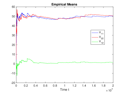
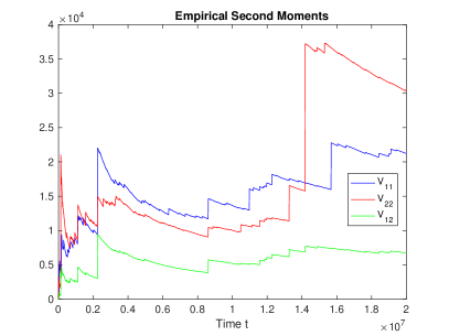
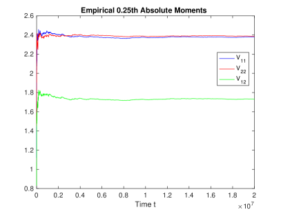
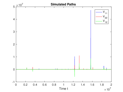
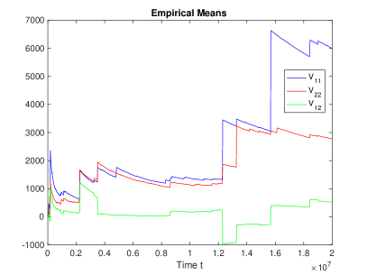
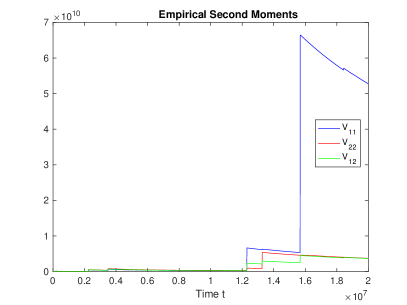
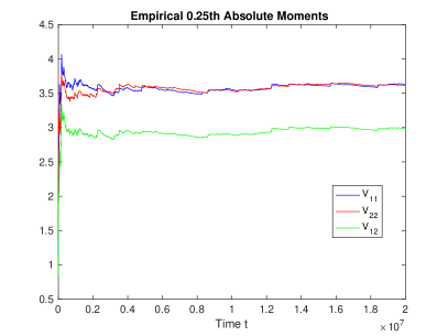
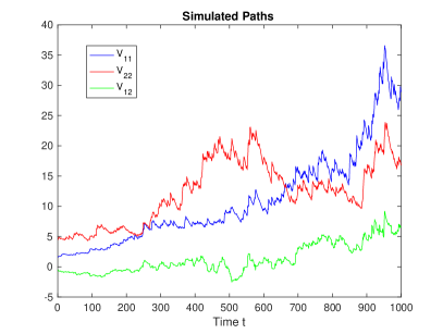
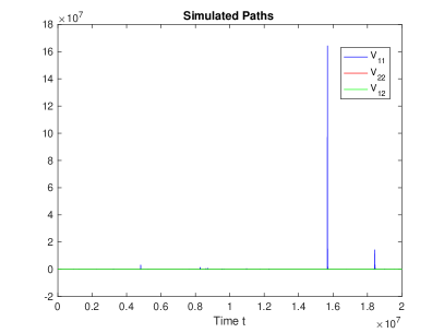
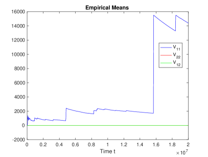
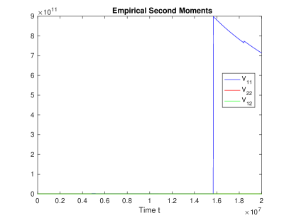
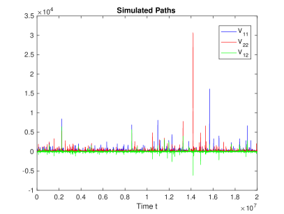
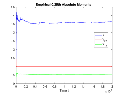
Figure 1: Plots of the simulations of Example 4.14 for α=0.14𝛼0.14\alpha=0.14. The first variance component (V11subscript𝑉11V_{11}) is depicted in blue, the second (V22subscript𝑉22V_{22}) in red and the covariance component (V12subscript𝑉12V_{12}) in green. The time horizon is zero to 20 million.
Refer to caption
Refer to caption
Refer to caption
Refer to caption
Figure 2: Plots of the simulations of Example 4.14 for α=0.142𝛼0.142\alpha=0.142. The first variance component (V11subscript𝑉11V_{11}) is depicted in blue, the second (V22subscript𝑉22V_{22}) in red and the covariance component (V12subscript𝑉12V_{12}) in green. The time horizon is zero to 20 million.
Refer to caption
Refer to caption
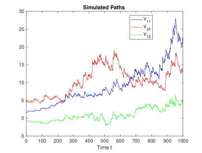
Figure 3: Plots of the simulations of Example 4.14, α=0.14𝛼0.14\alpha=0.14 on the left and α=0.142𝛼0.142\alpha=0.142 on the right. The first variance component (V11subscript𝑉11V_{11}) is depicted in blue, the second (V22subscript𝑉22V_{22}) in red and the covariance component (V12subscript𝑉12V_{12}) in green. The time horizon is zero to 1000.

Then condition (4.1) (or (4.2)) is satisfied (but not conditions (4.3), (4.4), (4.5)) and so we have geometric ergodicity with convergence of the (absolute) first moment. However, this is a rather extreme case as (given all the other parameter choices) (4.1) is satisfied if and only if |α|<0.020.1414𝛼0.020.1414|\alpha|<\sqrt{0.02}\approx 0.1414 and thus some convergences are only to be seen clearly for very long paths. We have simulated a path up to time 20 million with Matlab (see Figure 1). The paths themselves look immediately stationary (at this time scale) but extremely heavy tailed. In the long run (and not too fast) the running empirical means are reasonably converging (to their true values of 50 for the variances and 0 for the covariance). In sharp contrast to this there seems to be no convergence for the empirical second moments at all and actually we strongly conjecture that the stationary covariance matrix is infinite in this case. Looking at lower moments, like the 0.25th (absolute) empirical moments there is again convergence to be seen which is faster than the one for the first moment (as is to be expected). Zooming into the paths at the beginning in Figure 3 (left plot) shows that the process clearly does not start of like a stationary one, but the behaviour looks stationary to the eye very soon.

Changing only the parameter α𝛼\alpha to 0.1420.1420.142 and using the same random numbers we obtain the results depicted in Figure 2. The initial part of the paths (see right plot in Figure 3) looks almost unchanged (observe that the scaling of the vertical axes in the plots of Figure 2 differs). The paths in total clearly appear to be even more heavy tailed. Now neither the empirical second moments nor the empirical means seem to converge (and we conjecture that both mean and variance are infinite for the stationary distribution) . Now condition (4.1) does not hold any more and so the simulations suggest that this condition implying geometric ergodicity with convergence of the first moments is pretty sharp, as expected from the theoretical insight. The simulations also seem to clearly indicate that the 1/4th (absolute) moments still converge. Numerical integration shows for (4.3) (again the choice of η𝜂\eta makes no difference in this special case):

2((1+α2y22)141)νL(dy)+2β/40.00980.005>0.subscriptsuperscript2superscript1superscript𝛼2subscriptsuperscriptnorm𝑦22141subscript𝜈𝐿𝑑𝑦2𝛽40.00980.0050\int_{\mathbb{R}^{2}}\left(\left(1+\alpha^{2}\|y\|^{2}_{2}\right)^{\frac{1}{4}}-1\right)\nu_{L}(dy)+2\beta/4\approx 0.0098-0.005>0.

So our sufficient condition (4.3) for convergence of the 1/4141/4th moment is not satisfied, but due to the involved inequalities we expected it not to be too sharp. Actually, numerically not even the logarithmic condition [67, (4.3)] for the existence of a stationary distribution seems to be satisfied. This illustrates that these conditions involving norm estimates are not too sharp, as our simulations and the fact that condition (4.1) is almost satisfied strongly indicate that geometric ergodicity with convergence of some moments 0<p<10𝑝10<p<1 should hold.

Finally, we consider an example illustrating that our conditions for p1𝑝1p\not=1 are more precise if one coordinate dominates the others.

Example 4.15.

We consider the same model as in the previous Example 4.14 with the only difference that we now assume the jumps to have a two-dimensional normal distribution with covariance matrix ΣL=(100σ)subscriptΣ𝐿matrix100𝜎\Sigma_{L}=\begin{pmatrix}1&0\\ 0&\sigma\end{pmatrix} for σ>0𝜎0\sigma>0. For σ0𝜎0\sigma\to 0 we conclude from the formulae given in Example 4.10 that for p=1𝑝1p=1 (4.3), (4.4), (4.5) are asymptotically equivalent to (4.1) and as in Example 4.14 the choice of η𝜂\eta does not matter (they also are equivalent to (4.2) for η=I2𝜂subscript𝐼2\eta=I_{2}, but there the choice of η𝜂\eta may now matter). Note that (4.1) is not affected by changes in σ𝜎\sigma as long as σ1𝜎1\sigma\leq 1.

Choosing σ=1/1000𝜎11000\sigma=1/1000 and α=0.142𝛼0.142\alpha=0.142 as in the second part of Example 4.14 numerical integration shows for (4.3) with p=1/4𝑝14p=1/4:

2((1+α2y22)141)νL(dy)+2β/40.00490.005<0.subscriptsuperscript2superscript1superscript𝛼2subscriptsuperscriptnorm𝑦22141subscript𝜈𝐿𝑑𝑦2𝛽40.00490.0050\int_{\mathbb{R}^{2}}\left(\left(1+\alpha^{2}\|y\|^{2}_{2}\right)^{\frac{1}{4}}-1\right)\nu_{L}(dy)+2\beta/4\approx 0.0049-0.005<0.

So we obtain geometric ergodicity and the finiteness of the 1/4141/4th absolute moments from our theory.
Refer to caption
Refer to caption
Refer to caption
Refer to caption
Figure 4: Plots of the simulations of Example 4.15. The first variance component (V11subscript𝑉11V_{11}) is depicted in blue, the second (V22subscript𝑉22V_{22}) in red and the covariance component (V12subscript𝑉12V_{12}) in green. The time horizon is zero to 20 million.

Figure 4 shows the results of a simulation using the same time horizon and random numbers as in Example 4.14. The plots of the paths, the empirical means and second moments) show that the first variance component extremely dominates the others. One immediately sees that the empirical mean and second moment of V11subscript𝑉11V_{11} does not converge. In line with our theory all 0.25th absolute moments seem to converge pretty fast.

5 Irreducibility and aperiodicity of the MUCOGARCH volatility process

So far we have assumed away the issue of irreducibility and aperiodicity focusing on establishing a Foster-Lyapunov drift condition to obtain geometric ergodicity. As this is intrinsically related to the question of the existence of transition densities and support theorems, this is a very hard problem of its own. In our case the degeneracy of the noise, i.e. that all jumps of the Lévy process are rank one and that thus the jump distribution has no absolutely continuous component, makes our case particularly challenging.

We now establish sufficient conditions for the irreducibility and aperiodicity of Y𝑌Y by combining at least d𝑑d jumps to get an absolutely continuous component of the increments.

Theorem 5.1 (Irreducibility and Aperiodicity).

Let Y𝑌Y be a MUCOGARCH volatility process driven by a compound Poisson process L𝐿L and with AGLd()𝐴𝐺subscript𝐿𝑑A\in GL_{d}(\mathbb{R}), Re(σ(B))<0Re𝜎𝐵0\operatorname{Re}(\sigma(B))<0. If the jump distribution of L𝐿L has a non-trivial absolutely continuous component equivalent to the Lebesgue measure on dsuperscript𝑑\mathbb{R}^{d}, then Y𝑌Y is irreducible with respect to the Lebesgue measure on 𝕊d+superscriptsubscript𝕊𝑑\mathbb{S}_{d}^{+} and aperiodic.

We can soften the conditions on the jump distribution of the Compound Poisson process:

Corollary 5.2.

Let Y𝑌Y be a MUCOGARCH volatility process driven by a compound Poisson process L𝐿L and with AGLd()𝐴𝐺subscript𝐿𝑑A\in GL_{d}(\mathbb{R}), Re(σ(B))<0Re𝜎𝐵0\operatorname{Re}(\sigma(B))<0. If the jump distribution of L𝐿L has a non-trivial absolutely continuous component equivalent to the Lebesgue measure on dsuperscript𝑑\mathbb{R}^{d} restricted to an open neighborhood of zero, then Y𝑌Y is irreducible w.r.t. the Lebesgue measure restricted to an open neighborhood of zero in 𝕊d+superscriptsubscript𝕊𝑑\mathbb{S}_{d}^{+} and aperiodic.

Remark 5.3.

(i) If the driving Lévy process is an infinite activity Lévy process, whose Lévy measure has a non-trivial absolutely continuous component and the density of the component w.r.t. the Lebesgue measure on 𝕊d+superscriptsubscript𝕊𝑑\mathbb{S}_{d}^{+} is strictly positive in a neighborhood of zero, we can show that Y𝑌Y is open-set irreducible w.r.t. the Lebesgue measure restricted to an open neighborhood of zero in 𝕊d+superscriptsubscript𝕊𝑑{\mathbb{S}_{d}^{+}}. For strong Feller processes open-set irreducibility provides irreducibility, but the strong Feller property is to the best of our knowledge hard to establish for Lévy-driven SDEs. A classical way to show irreducibility is by using density or support theorems based on Malliavin Calculus, see e.g. [20, 44, 65]. But they all require, that the coefficients of the SDE have bounded derivatives, which is not the case for the MUCOGARCH volatility process. So finding criteria for irreducibility in the infinite activity case appears to be a very challenging question beyond the scope of the present paper.

(ii) In the univariate case establishing irreducibility and aperiodicity is much easier, as one can easily use the explicit representation of the COGARCH(1,1) volatility process to establish that one has weak convergence to a unique stationary distribution which is self-decomposable and thus has a strictly positive density. This way is blocked in the multivariate case as we do not have the explicit representation and the linear recurrence equation structure.

Note that the condition that the Lévy measure has an absolutely continuous component with a support containing zero is the obvious analogue to the condition on the noise in [14].

Remark 5.4.

Let us return to the SDE (4.8) driven by a general matrix subordinator which we introduced in Remark 4.12. It is straightforward to see that then the conclusions of Theorem 5.1 or Corollary 5.2, respectively, are valid for the process Y𝑌Y, if the matrix subordinator L𝐿L is a compound Poisson process with the jump distribution of L𝐿L having a non-trivial absolutely continuous component equivalent to the Lebesgue measure on 𝕊d+superscriptsubscript𝕊𝑑\mathbb{S}_{d}^{+} (restricted to an open neighborhood of zero).

6 Proofs

To prove our results we use the stability concepts for Markov processes of [52, 53].

6.1 Markov processes and ergodicity

For the convenience of the reader, we first give a short introduction to the definitions and results for general continuous time Markov processes following mainly [25, Section 3].

Given be a state space X𝑋X, which is assumed to be an open or closed subset of a finite-dimensional real vector spaced equipped with the usual topology and the Borel-σ𝜎\sigma-algebra (X)𝑋\mathcal{B}(X). We consider a continuous time Markov process Φ=(Φt)t0ΦsubscriptsubscriptΦ𝑡𝑡0\Phi=(\Phi_{t})_{t\geq 0} on X𝑋X with transition probabilities t(x,A)=x(ΦtA)superscript𝑡𝑥𝐴subscript𝑥subscriptΦ𝑡𝐴\mathbb{P}^{t}(x,A)=\mathbb{P}_{x}(\Phi_{t}\in A) for xX,A(X)formulae-sequence𝑥𝑋𝐴𝑋x\in X,A\in\mathcal{B}(X).

The operator tsuperscript𝑡\mathbb{P}^{t} from the associated transition semigroup acts on a bounded measurable function f𝑓f as

tf(x)=Xt(x,dy)f(y)superscript𝑡𝑓𝑥subscript𝑋superscript𝑡𝑥𝑑𝑦𝑓𝑦\mathbb{P}^{t}f(x)=\int_{X}\mathbb{P}^{t}(x,dy)f(y) (6.1)

and on a σ𝜎\sigma-finite measure μ𝜇\mu on X𝑋X as

μt(A)=Xμ(dy)t(y,A).𝜇superscript𝑡𝐴subscript𝑋𝜇𝑑𝑦superscript𝑡𝑦𝐴\mu\mathbb{P}^{t}(A)=\int_{X}\mu(dy)\mathbb{P}^{t}(y,A). (6.2)

To define non-explosivity, we consider a fixed family {On|n+}conditional-setsubscript𝑂𝑛𝑛subscript\{O_{n}|n\in\mathbb{Z}_{+}\} of open precompact sets, i.e. the closure of Onsubscript𝑂𝑛O_{n} is a compact subset of X𝑋X, for which OnXsubscript𝑂𝑛𝑋O_{n}\nearrow X as n𝑛n\to\infty. With Tmsuperscript𝑇𝑚T^{m} we denote the first entrance time to Omcsuperscriptsubscript𝑂𝑚𝑐O_{m}^{c} and by ξ𝜉\xi the exit time for the process, defined as ξ=𝒟limmTm.𝜉𝒟subscript𝑚superscript𝑇𝑚\xi\overset{\mathcal{D}}{=}\lim_{m\to\infty}T^{m}.

Definition 6.1 (Non-explosivity, [53, Chapter 1.2]).

We call the process ΦΦ\Phi non-explosive if x(ξ=)=1subscript𝑥𝜉1\mathbb{P}_{x}(\xi=\infty)=1 for all xX𝑥𝑋x\in X.

By 𝒞b(X)subscript𝒞𝑏𝑋\mathcal{C}_{b}(X) we denote the set of all continuous and bounded functions f:X:𝑓𝑋f:X\to\mathbb{R} and by 𝒞0(X)subscript𝒞0𝑋\mathcal{C}_{0}(X) those continuous and bounded functions, which vanish at infinity.

Definition 6.2 (Stochastic continuity and Feller processes).

Let (t)t+subscriptsuperscript𝑡𝑡subscript(\mathbb{P}^{t})_{t\in\mathbb{R}_{+}} be the transition semigroup of a time homogeneous Markov process ΦΦ\Phi.
(i) (t)t+subscriptsuperscript𝑡𝑡subscript(\mathbb{P}^{t})_{t\in\mathbb{R}_{+}} or ΦΦ\Phi is called stochastically continuous if

limt0t0t(x,𝒩(x))=1subscript𝑡0𝑡0superscript𝑡𝑥𝒩𝑥1\lim_{\begin{subarray}{c}t\to 0\\ t\geq 0\end{subarray}}\mathbb{P}^{t}(x,\mathcal{N}(x))=1 (6.3)

for all xX𝑥𝑋x\in X and open neighborhoods 𝒩(x)𝒩𝑥\mathcal{N}(x) of x𝑥x.
(ii) (t)t+subscriptsuperscript𝑡𝑡subscript(\mathbb{P}^{t})_{t\in\mathbb{R}_{+}} or ΦΦ\Phi is a (weak) 𝒞bsubscript𝒞b\mathbf{\mathcal{C}_{b}}-Feller semigroup or process if it is stochastically continuous and

t(𝒞b(X))𝒞b(X) for all t0.superscript𝑡subscript𝒞𝑏𝑋subscript𝒞𝑏𝑋 for all 𝑡0\mathbb{P}^{t}(\mathcal{C}_{b}(X))\subseteq\mathcal{C}_{b}(X)\text{ for all }t\geq 0.\\ (6.4)

(iii) If in (ii) we have instead of (6.4)

t(𝒞0(X))𝒞0(X) for all t0superscript𝑡subscript𝒞0𝑋subscript𝒞0𝑋 for all 𝑡0\mathbb{P}^{t}(\mathcal{C}_{0}(X))\subseteq\mathcal{C}_{0}(X)\text{ for all }t\geq 0 (6.5)

we call the semigroup or the process (weak) 𝒞0subscript𝒞0\mathbf{\mathcal{C}_{0}}-Feller.

Combining the definition of strongly continuous contraction semigroups, Theorem 4.1.1 and the definition of Feller processes in [48] shows that a 𝒞0subscript𝒞0{\mathcal{C}_{0}}-Feller process is a Borel-right process (cf. [48] for a definition).

From now on we assume that ΦΦ\Phi is a non-explosive Borel right process. For the definitions and details of the existence and structure see [64].

Definition 6.3 (Invariant measure, [25, Chapter 3 ]).

A σ𝜎\sigma-finite measure π𝜋\pi on (X)𝑋\mathcal{B}(X) with the property

π=πt,t0formulae-sequence𝜋𝜋superscript𝑡for-all𝑡0\pi=\pi\mathbb{P}^{t},\ \forall t\geq 0 (6.6)

is called invariant.

Notation: By π𝜋\pi we always denote an invariant measure of ΦΦ\Phi, if it exists.

Definition 6.4 (Exponential ergodicity, [25, Chapter 3 ]).

ΦΦ\Phi is called exponentially ergodic, if an invariant measure π𝜋\pi exists and satisfies for all xX𝑥𝑋x\in X

t(x,.)πTVM(x)ρt,t0\|\mathbb{P}^{t}(x,.)-\pi\|_{\text{TV}}\leq M(x)\rho^{t},\ \ \forall t\geq 0 (6.7)

for some finite M(x)𝑀𝑥M(x), some ρ<1𝜌1\rho<1 and where μTV:=sup|g|1,g measurable|μ(dy)g(y)|assignsubscriptnorm𝜇TVsubscriptsupremum𝑔1𝑔 measurable𝜇𝑑𝑦𝑔𝑦\|\mu\|_{\text{TV}}:=\sup_{|g|\leq 1,\,g\text{ measurable}}|\int\mu(dy)g(y)| denotes the total variation norm.

If this convergence holds for the f𝑓f-norm μf:=sup|g|f,g measurable|μ(dy)g(y)|assignsubscriptnorm𝜇𝑓subscriptsupremum𝑔𝑓𝑔 measurable𝜇𝑑𝑦𝑔𝑦\|\mu\|_{f}:=\sup_{|g|\leq f,\,g\text{ measurable}}|\int\mu(dy)g(y)| (for any signed measure μ𝜇\mu) , where f𝑓f is a measurable function from the state space X𝑋X to [1,)1[1,\infty), we call the process 𝐟𝐟\mathbf{f}-exponentially ergodic.

A seemingly stronger formulation of V𝑉V-exponential ergodicity is V𝑉V-uniform ergodicity: We require that M(x)=V(x)D𝑀𝑥𝑉𝑥𝐷M(x)=V(x)\cdot D with some finite constant D𝐷D.

Definition 6.5 (V𝑉V-uniform ergodicity, [25, Chapter 3]).

ΦΦ\Phi is called 𝐕𝐕\mathbf{V}-uniformly ergodic, if a measurable function V:X[1,):𝑉𝑋1V:X\to[1,\infty) exists such that for all xX𝑥𝑋x\in X

t(x,.)πVV(x)Dρt,t0\|\mathbb{P}^{t}(x,.)-\pi\|_{V}\leq V(x)D\rho^{t},\ t\geq 0 (6.8)

holds for some D<,ρ<1formulae-sequence𝐷𝜌1D<\infty,\rho<1.

To prove ergodicity we need the notions of irreducibility and aperiodicity.

Definition 6.6 ([25], Chapter 3).

For any σ𝜎\sigma-finite measure μ𝜇\mu on (X)𝑋\mathcal{B}(X) we call the process ΦΦ\Phi 𝛍𝛍\mu-irreducible if for any B(X)𝐵𝑋B\in\mathcal{B}(X) with μ(B)>0𝜇𝐵0\mu(B)>0

𝔼x(ηB)>0,xXformulae-sequencesubscript𝔼𝑥subscript𝜂𝐵0for-all𝑥𝑋\mathbb{E}_{x}(\eta_{B})>0,\forall x\in X (6.9)

holds, where ηB:=0𝟙{ΦtB}𝑑tassignsubscript𝜂𝐵superscriptsubscript0subscript1subscriptΦ𝑡𝐵differential-d𝑡\eta_{B}:=\int_{0}^{\infty}\mathds{1}_{\{\Phi_{t}\in B\}}dt is the occupation time.

This is obviously the same as requiring

0t(x,B)𝑑t>0,xX.formulae-sequencesuperscriptsubscript0superscript𝑡𝑥𝐵differential-d𝑡0for-all𝑥𝑋\int_{0}^{\infty}\mathbb{P}^{t}(x,B)dt>0,\ \forall x\in X. (6.10)

If ΦΦ\Phi is μ𝜇\mu-irreducible, there exists a maximal irreducibility measure ψ𝜓\psi such that every other irreducibility measure ν𝜈\nu is absolutely continuous with respect to ψ𝜓\psi (see [52, p. 493]). We write 𝓑+(𝑿)superscript𝓑𝑿\boldsymbol{\mathcal{B}^{+}(X)} for the collection of all measurable subsets A(X)𝐴𝑋A\in\mathcal{B}(X) with ψ(A)>0𝜓𝐴0\psi(A)>0.

Remark 6.7.

In [69, Proposition 1.1] it was shown, that if the discrete time hh-skeleton of a process, the hsuperscript\mathbb{P}^{h}-chain, is ψ𝜓\psi-irreducible for some h>00h>0, then it holds for the continuous time process. If the hsuperscript\mathbb{P}^{h}-chain is ψ𝜓\psi-irreducible for every h>00h>0, we call the process simultaneously 𝛙𝛙\boldsymbol{\psi}-irreducible.

One probabilistic form of stability is the concept of Harris recurrence.

Definition 6.8 (Harris recurrence, [52, Chapter 2.2]).

(i) ΦΦ\Phi is called Harris recurrent, if either

  • x(ηA=)=1subscript𝑥subscript𝜂𝐴1\mathbb{P}_{x}(\eta_{A}=\infty)=1 whenever ϕ(A)>0italic-ϕ𝐴0\phi(A)>0 for some σ𝜎\sigma-finite measure ϕitalic-ϕ\phi, or

  • x(τA<)=1subscript𝑥subscript𝜏𝐴1\mathbb{P}_{x}(\tau_{A}<\infty)=1 whenever μ(A)>0𝜇𝐴0\mu(A)>0 for some σ𝜎\sigma-finite measure μ𝜇\mu. τA:=inf{t0:ΦtA}assignsubscript𝜏𝐴infimumconditional-set𝑡0subscriptΦ𝑡𝐴\tau_{A}:=\inf\{t\geq 0\leavevmode\nobreak\ :\leavevmode\nobreak\ \Phi_{t}\in A\} is the first hitting time of A𝐴A.

(ii) Suppose that ΦΦ\Phi is Harris recurrent with finite invariant measure π𝜋\pi, then ΦΦ\Phi is called positive Harris recurrent.

To define the class of subsets of X𝑋X called petite sets, we suppose that a𝑎a is a probability distribution on +subscript\mathbb{R}_{+}. We define the Markov transition function Kasubscript𝐾𝑎K_{a} for the process sampled by a𝑎a as

Ka(x,A):=0t(x,A)a(dt),xX,A.formulae-sequenceassignsubscript𝐾𝑎𝑥𝐴superscriptsubscript0superscript𝑡𝑥𝐴𝑎𝑑𝑡formulae-sequencefor-all𝑥𝑋𝐴K_{a}(x,A):=\int_{0}^{\infty}\mathbb{P}^{t}(x,A)a(dt),\ \forall x\in X,A\in\mathcal{B}. (6.11)
Definition 6.9 (Petite and small sets, [25, Chapter 3]).

A nonempty set C𝐶C\in\mathcal{B} is called 𝛎𝐚subscript𝛎𝐚\boldsymbol{\nu_{a}}-petite, if νasubscript𝜈𝑎\nu_{a} is a nontrivial measure on (X)𝑋\mathcal{B}(X) and a𝑎a is a sampling distribution on (0,)0(0,\infty) satisfying

Ka(x,.)νa(.),xC.K_{a}(x,.)\geq\nu_{a}(.),\ \forall x\in C. (6.12)

When the sampling distribution a𝑎a is degenerate, i.e. a single point mass, we call the set C𝐶C small.

Remark 6.10.

Like in the discrete time Markov chain theory the set C𝐶C is small, if there exists an m>0𝑚0m>0 and a nontrivial measure νmsubscript𝜈𝑚\nu_{m} on (X)𝑋\mathcal{B}(X) such that for all xC,B(X)formulae-sequence𝑥𝐶𝐵𝑋x\in C,B\in\mathcal{B}(X)

m(x,B)νm(B)superscript𝑚𝑥𝐵subscript𝜈𝑚𝐵\mathbb{P}^{m}(x,B)\geq\nu_{m}(B) (6.13)

holds.

For discrete time chains there exists a well known concept of periodicity, see for example [54, Chapter 5.4]. For continuous time processes this definition is not adaptable, since there are no fixed time steps. But a similar concept is the definition of aperiodicity for continuous time Markov processes as introduced in [25].

Definition 6.11 ([25], Chapter 3).

A ψ𝜓\psi-irreducible Markov process is called aperiodic if for some small set C+(X)𝐶superscript𝑋C\in\mathcal{B}^{+}(X) there exists a T𝑇T such that t(x,C)>0superscript𝑡𝑥𝐶0\mathbb{P}^{t}(x,C)>0 for all tT𝑡𝑇t\geq T and all xC𝑥𝐶x\in C.

Proposition 6.12.

When ΦΦ\Phi is simultaneously ψ𝜓\psi-irreducible then we know from [69, Proposition 1.2] that every skeleton chain is aperiodic in the sense of a discrete time Markov chain.

For discrete time Markov processes there exist conditions such that every compact set is petite and every petite set is small:

Proposition 6.13 ([54], Theorem 6.0.1 and 5.5.7).

(i) If ΦΦ\Phi, a discrete time Markov process, is a ΨΨ\Psi-irreducible Feller chain with supp(Ψ)𝑠𝑢𝑝𝑝Ψsupp(\Psi) having non-empty interior, every compact set is petite.
(ii)  If ΦΦ\Phi is irreducible and aperiodic, then every petite set is small.

Remark 6.14.

Proposition 6.13 (i) is also true for continuous time Markov processes, see [52].

To introduce the Foster-Lyapunov criterion for ergodicity we need the concept of the extended generator of a Markov process.

Definition 6.15 (Extended generator, [25, Chapter 4]).

𝒟(𝒜)𝒟𝒜\mathcal{D}(\mathcal{A}) denotes the set of all functions f:X×+:𝑓𝑋subscriptf:X\times\mathbb{R}_{+}\to\mathbb{R} for which a function g:X×+:𝑔𝑋subscriptg:X\times\mathbb{R}_{+}\to\mathbb{R} exists, such that xX,t>0formulae-sequencefor-all𝑥𝑋𝑡0\forall x\in X,t>0

𝔼x(f(Φt,t))=f(x,0)+𝔼x(0tg(Φs,s)𝑑s),subscript𝔼𝑥𝑓subscriptΦ𝑡𝑡𝑓𝑥0subscript𝔼𝑥superscriptsubscript0𝑡𝑔subscriptΦ𝑠𝑠differential-d𝑠\displaystyle\mathbb{E}_{x}(f(\Phi_{t},t))=f(x,0)+\mathbb{E}_{x}\left(\int_{0}^{t}g(\Phi_{s},s)ds\right), (6.14)
𝔼x(0t|g(Φs,s)|𝑑s)<subscript𝔼𝑥superscriptsubscript0𝑡𝑔subscriptΦ𝑠𝑠differential-d𝑠\displaystyle\mathbb{E}_{x}\left(\int_{0}^{t}|g(\Phi_{s},s)|ds\right)<\infty (6.15)

holds. We write 𝓐𝐟:=𝐠assign𝓐𝐟𝐠\mathcal{A}f:=g and call 𝒜𝒜\mathcal{A} the extended generator of ΦΦ\Phi. 𝒟(𝒜)𝒟𝒜\mathcal{D}(\mathcal{A}) is called the domain of 𝒜𝒜\mathcal{A}.

The next theorem from [25] gives for an irreducible and aperiodic Markov process a sufficient criterion to be V𝑉V-uniformly ergodic. This is a modification of the Foster-Lyapunov drift criterion of [53].

Theorem 6.16 ([25], Theorem 5.2).

Let (Φt)t0subscriptsubscriptΦ𝑡𝑡0(\Phi_{t})_{t\geq 0} be a μ𝜇\mu-irreducible and aperiodic Markov process. If there exist constants b,c>0𝑏𝑐0b,c>0 and a petite set C𝐶C in (X)𝑋\mathcal{B}(X) as well as a measurable function V:X[1,):𝑉𝑋1V:X\to[1,\infty) such that

𝒜VbV+c𝟙C,𝒜𝑉𝑏𝑉𝑐subscript1𝐶\mathcal{A}V\leq-bV+c\mathds{1}_{C}, (6.16)

where 𝒜𝒜\mathcal{A} is the extended generator, then (Φt)t0subscriptsubscriptΦ𝑡𝑡0(\Phi_{t})_{t\geq 0} is V𝑉V-uniformly ergodic.

6.2 Proofs of Section 4

We prove the geometric ergodicity of the MUCOGARCH volatility process by using Theorem 6.16. The main task is to show the validity of a Foster-Lyapunov drift condition and that the used function belongs to the domain of the extended generator. For the latter we need the existence of moments given in Lemma 4.2. The different steps require similar inequalities. The most precise estimations are needed for the Foster-Lyapunov drift condition. Therefore we below first prove the Forster-Lyapunov drift condition assuming for a moment that we are in the domain of the extended generator and prove this and the finiteness of moments later on, as the inequalities needed there are often obvious from the proof of the Foster-Lyapunov drift condition.

6.2.1 Proof of Theorem 4.3

The first and main part of the proof is to show the geometric ergodicity, as the positive Harris recurrence is essentially a consequence of it. To prove the geometric ergodicity, and hence the existence and uniqueness of a stationary distribution, of the MUCOGARCH volatility process, it is enough to show that the Foster-Lyapunov drift condition of Theorem 6.16 holds. All other conditions of Theorem 6.16 follow from Theorem 3.3 or the assumptions.

The extended generator

Using e.g. the results on SDEs, the stochastic symbol and the infinitesimal generator of [63, Chapter 6.1], [63, Chapter 6.1] and [62, Theorem 3.1] and that tr(XY)tr𝑋𝑌\operatorname{tr}(XY) is the canonical scalar product in 𝕊dsubscript𝕊𝑑\mathbb{S}_{d}, we see that for a sufficiently regular function u:𝕊d+:𝑢superscriptsubscript𝕊𝑑u:\mathbb{S}_{d}^{+}\to\mathbb{R} in the domain of the (extended/infinitesimal) generator 𝒜𝒜\mathcal{A} we have.

𝒜u(x)𝒜𝑢𝑥\displaystyle\mathcal{A}u(x) =tr((Bx+xB)u(x))+d(u(x+A(C+x)1/2yy(C+x)1/2A)u(x))νL(dy)absenttr𝐵𝑥𝑥superscript𝐵top𝑢𝑥subscriptsuperscript𝑑𝑢𝑥𝐴superscript𝐶𝑥12𝑦superscript𝑦topsuperscript𝐶𝑥12superscript𝐴top𝑢𝑥subscript𝜈𝐿𝑑𝑦\displaystyle=\operatorname{tr}\left((Bx+xB^{\top})\nabla u(x)\right)+\int_{\mathbb{R}^{d}}\left(u(x+A(C+x)^{1/2}yy^{\top}(C+x)^{1/2}A^{\top})-u(x)\right)\nu_{L}(dy)
=:𝒟u(x)+𝒥u(x).\displaystyle=:\mathcal{D}u(x)+\mathcal{J}u(x).

We abbreviate the first addend, the drift part, with 𝒟u(x)𝒟𝑢𝑥\mathcal{D}u(x) and the second, the jump part, with 𝒥u(x)𝒥𝑢𝑥\mathcal{J}u(x).

Foster-Lyapunov drift inequality

As test function we choose u(x)=tr(ηx)p+1u(x)=\operatorname{tr}(\eta x)^{p}+1, thus u(x)1𝑢𝑥1u(x)\geq 1. Note that the gradient of u𝑢u is given by u(x)=ptr(ηx)p1η\nabla u(x)=p\operatorname{tr}(\eta x)^{p-1}\eta.

For p(0,1)𝑝01p\in(0,1) the gradient of u𝑢u has a singularity in 00, but in the end we look at tr((Bx+xB)u(x))tr𝐵𝑥𝑥superscript𝐵top𝑢𝑥\operatorname{tr}\left((Bx+xB^{\top})\nabla u(x)\right), which turns out to be continuous in 00.

Now we need to look at the cases (i) - (v) separately, as the proofs work along similar lines, but differ in important details.

Case (i)

We have

𝒥u(x)𝒥𝑢𝑥\displaystyle\mathcal{J}u(x) =d(tr(η(x+A(C+x)1/2yy(C+x)1/2A))tr(ηx))νL(dy)absentsubscriptsuperscript𝑑tr𝜂𝑥𝐴superscript𝐶𝑥12𝑦superscript𝑦topsuperscript𝐶𝑥12superscript𝐴toptr𝜂𝑥subscript𝜈𝐿𝑑𝑦\displaystyle=\int_{\mathbb{R}^{d}}\left(\operatorname{tr}\left(\eta(x+A(C+x)^{1/2}yy^{\top}(C+x)^{1/2}A^{\top})\right)-\operatorname{tr}\left(\eta x\right)\right)\nu_{L}(dy)
=dtr(η1/2A(C+x)1/2yy(C+x)1/2Aη1/2)νL(dy)absentsubscriptsuperscript𝑑trsuperscript𝜂12𝐴superscript𝐶𝑥12𝑦superscript𝑦topsuperscript𝐶𝑥12superscript𝐴topsuperscript𝜂12subscript𝜈𝐿𝑑𝑦\displaystyle=\int_{\mathbb{R}^{d}}\operatorname{tr}\left(\eta^{1/2}A(C+x)^{1/2}yy^{\top}(C+x)^{1/2}A^{\top}\eta^{1/2}\right)\nu_{L}(dy)
=tr(η1/2A(C+x)1/2dyyνL(dy)(C+x)1/2Aη1/2)absenttrsuperscript𝜂12𝐴superscript𝐶𝑥12subscriptsuperscript𝑑𝑦superscript𝑦topsubscript𝜈𝐿𝑑𝑦superscript𝐶𝑥12superscript𝐴topsuperscript𝜂12\displaystyle=\operatorname{tr}\left(\eta^{1/2}A(C+x)^{1/2}\int_{\mathbb{R}^{d}}yy^{\top}\nu_{L}(dy)(C+x)^{1/2}A^{\top}\eta^{1/2}\right)
tr(η1/2A(C+x)Aη1/2)dyyνL(dy)2.absenttrsuperscript𝜂12𝐴𝐶𝑥superscript𝐴topsuperscript𝜂12subscriptnormsubscriptsuperscript𝑑𝑦superscript𝑦topsubscript𝜈𝐿𝑑𝑦2\displaystyle\leq\operatorname{tr}\left(\eta^{1/2}A(C+x)A^{\top}\eta^{1/2}\right)\left\|\int_{\mathbb{R}^{d}}yy^{\top}\nu_{L}(dy)\right\|_{2}.

In the last step we used XX2Id=λmax(X)Idprecedes-or-equals𝑋subscriptnorm𝑋2subscript𝐼𝑑subscript𝜆𝑚𝑎𝑥𝑋subscript𝐼𝑑X\preceq\|X\|_{2}I_{d}=\lambda_{max}(X)I_{d} for X𝕊d+𝑋superscriptsubscript𝕊𝑑X\in\mathbb{S}_{d}^{+}, that trtr\operatorname{tr} is monotone in the natural order on 𝕊d+superscriptsubscript𝕊𝑑\mathbb{S}_{d}^{+}, and that maps of the form 𝕊d𝕊d,XZXZformulae-sequencesubscript𝕊𝑑subscript𝕊𝑑maps-to𝑋𝑍𝑋superscript𝑍top\mathbb{S}_{d}\to\mathbb{S}_{d},X\mapsto ZXZ^{\top} with ZMd()𝑍subscript𝑀𝑑Z\in M_{d}(\mathbb{R}) are order preserving.

Hence

𝒥u(x)𝒥𝑢𝑥\displaystyle\mathcal{J}u(x) tr(AηA(C+x))dyyνL(dy)2.absenttrsuperscript𝐴top𝜂𝐴𝐶𝑥subscriptnormsubscriptsuperscript𝑑𝑦superscript𝑦topsubscript𝜈𝐿𝑑𝑦2\displaystyle\leq\operatorname{tr}\left(A^{\top}\eta A(C+x)\right)\left\|\int_{\mathbb{R}^{d}}yy^{\top}\nu_{L}(dy)\right\|_{2}.

For the drift part we get

𝒟u(x)𝒟𝑢𝑥\displaystyle\mathcal{D}u(x) =tr((Bx+xB)η)=tr((ηB+Bη)x).absenttr𝐵𝑥𝑥superscript𝐵top𝜂tr𝜂𝐵superscript𝐵top𝜂𝑥\displaystyle=\operatorname{tr}\left((Bx+xB^{\top})\eta\right)=\operatorname{tr}((\eta B+B^{\top}\eta)x).

Together we have

𝒜u(x)𝒜𝑢𝑥\displaystyle\mathcal{A}u(x) =tr((ηB+Bη+AηAdyyνL(dy)2νL(dy))x)+tr(AηAC)dyyνL(dy)2.absenttr𝜂𝐵superscript𝐵top𝜂superscript𝐴top𝜂𝐴subscriptnormsubscriptsuperscript𝑑𝑦superscript𝑦topsubscript𝜈𝐿𝑑𝑦2subscript𝜈𝐿𝑑𝑦𝑥trsuperscript𝐴top𝜂𝐴𝐶subscriptnormsubscriptsuperscript𝑑𝑦superscript𝑦topsubscript𝜈𝐿𝑑𝑦2\displaystyle=\operatorname{tr}\left(\left(\eta B+B^{\top}\eta+A^{\top}\eta A\left\|\int_{\mathbb{R}^{d}}yy^{\top}\nu_{L}(dy)\right\|_{2}\nu_{L}(dy)\right)x\right)+\operatorname{tr}\left(A^{\top}\eta AC\right)\left\|\int_{\mathbb{R}^{d}}yy^{\top}\nu_{L}(dy)\right\|_{2}.

Since ηB+Bη+AηAdyyνL(dy)2𝕊d++𝜂𝐵superscript𝐵top𝜂superscript𝐴top𝜂𝐴subscriptnormsubscriptsuperscript𝑑𝑦superscript𝑦topsubscript𝜈𝐿𝑑𝑦2superscriptsubscript𝕊𝑑absent\eta B+B^{\top}\eta+A^{\top}\eta A\left\|\int_{\mathbb{R}^{d}}yy^{\top}\nu_{L}(dy)\right\|_{2}\in-\mathbb{S}_{d}^{++}, there exists a c>0𝑐0c>0, such that

tr((ηB+Bη+AηAdyyνL(dy)2)x)ctr(ηx).tr𝜂𝐵superscript𝐵top𝜂superscript𝐴top𝜂𝐴subscriptnormsubscriptsuperscript𝑑𝑦superscript𝑦topsubscript𝜈𝐿𝑑𝑦2𝑥𝑐tr𝜂𝑥\operatorname{tr}\left(\left(\eta B+B^{\top}\eta+A^{\top}\eta A\left\|\int_{\mathbb{R}^{d}}yy^{\top}\nu_{L}(dy)\right\|_{2}\right)x\right)\leq-c\operatorname{tr}(\eta x).

Summarizing we have that there exist c,d>0𝑐𝑑0c,d>0 such that

𝒜u(x)ctr(ηx)+d.𝒜𝑢𝑥𝑐tr𝜂𝑥𝑑\mathcal{A}u(x)\leq-c\operatorname{tr}(\eta x)+d. (6.17)

For tr(x)>ktr𝑥𝑘\operatorname{tr}(x)>k and k𝑘k big enough there exist 0<c1<c0subscript𝑐1𝑐0<c_{1}<c such that 𝒜u(x)c1(tr(ηx)+1).𝒜𝑢𝑥subscript𝑐1tr𝜂𝑥1\mathcal{A}u(x)\leq-c_{1}(\operatorname{tr}(\eta x)+1). For tr(x)ktr𝑥𝑘\operatorname{tr}(x)\leq k we have c1tr(ηx)+d=c1(tr(ηx)+1)+e,subscript𝑐1tr𝜂𝑥𝑑subscript𝑐1tr𝜂𝑥1𝑒-c_{1}\operatorname{tr}(\eta x)+d=-c_{1}(\operatorname{tr}(\eta x)+1)+e, with e:=c1+d>0assign𝑒subscript𝑐1𝑑0e:=c_{1}+d>0. Altogether we have

𝒜u(x)c1u(x)+e𝟙Dk,𝒜𝑢𝑥subscript𝑐1𝑢𝑥𝑒subscript1subscript𝐷𝑘\mathcal{A}u(x)\leq-c_{1}u(x)+e\mathds{1}_{D_{k}}, (6.18)

where Dk:={x:tr(x)k}assignsubscript𝐷𝑘conditional-set𝑥tr𝑥𝑘D_{k}:=\{x:\operatorname{tr}(x)\leq k\} is a compact set. By Proposition 6.13 (i) this is also a petite set. Therefore the Foster-Lyapunov drift condition is proved.

Case (ii)

Compared to Case (i) we just change the inequality for the jump part. Using Lemma 4.1 we have

𝒥u(x)𝒥𝑢𝑥\displaystyle\mathcal{J}u(x) =dtr(AηA(C+x)1/2yy(C+x)1/2)νL(dy)λmax(AηA)tr((C+x)dyyνL(dy))absentsubscriptsuperscript𝑑trsuperscript𝐴top𝜂𝐴superscript𝐶𝑥12𝑦superscript𝑦topsuperscript𝐶𝑥12subscript𝜈𝐿𝑑𝑦subscript𝜆𝑚𝑎𝑥superscript𝐴top𝜂𝐴tr𝐶𝑥subscriptsuperscript𝑑𝑦superscript𝑦topsubscript𝜈𝐿𝑑𝑦\displaystyle=\int_{\mathbb{R}^{d}}\operatorname{tr}\left(A^{\top}\eta A(C+x)^{1/2}yy^{\top}(C+x)^{1/2}\right)\nu_{L}(dy)\leq\lambda_{max}(A^{\top}\eta A)\operatorname{tr}\left((C+x)\int_{\mathbb{R}^{d}}yy^{\top}\nu_{L}(dy)\right)

and hence

𝒜u(x)𝒜𝑢𝑥\displaystyle\mathcal{A}u(x) =tr((ηB+Bη+λmax(AηA)dyyνL(dy))x)+λmax(AηA)tr(CdyyνL(dy)).absenttr𝜂𝐵superscript𝐵top𝜂subscript𝜆𝑚𝑎𝑥superscript𝐴top𝜂𝐴subscriptsuperscript𝑑𝑦superscript𝑦topsubscript𝜈𝐿𝑑𝑦𝑥subscript𝜆𝑚𝑎𝑥superscript𝐴top𝜂𝐴tr𝐶subscriptsuperscript𝑑𝑦superscript𝑦topsubscript𝜈𝐿𝑑𝑦\displaystyle=\operatorname{tr}\left(\left(\eta B+B^{\top}\eta+\lambda_{max}(A^{\top}\eta A)\int_{\mathbb{R}^{d}}yy^{\top}\nu_{L}(dy)\right)x\right)+\lambda_{max}(A^{\top}\eta A)\operatorname{tr}\left(C\int_{\mathbb{R}^{d}}yy^{\top}\nu_{L}(dy)\right).

Now we can proceed as before.

Cases (iii) and (iv)

We have for the drift part

𝒟u(x)𝒟𝑢𝑥\displaystyle\mathcal{D}u(x) =ptr((ηB+Bη)x)tr(ηx)p1Kη,Bptr(ηx)p.\displaystyle=p\operatorname{tr}((\eta B+B^{\top}\eta)x)\operatorname{tr}(\eta x)^{p-1}\leq K_{\eta,B}p\operatorname{tr}(\eta x)^{p}.

For the jump part we get using that yy2=y22subscriptnorm𝑦superscript𝑦top2superscriptsubscriptnorm𝑦22\|yy^{\top}\|_{2}=\|y\|_{2}^{2} for yd𝑦superscript𝑑y\in\mathbb{R}^{d}

𝒥u(x)𝒥𝑢𝑥\displaystyle\mathcal{J}u(x) =d(tr(η(x+A(C+x)1/2yy(C+x)1/2A))ptr(ηx)p)νL(dy)\displaystyle=\int_{\mathbb{R}^{d}}\left(\operatorname{tr}\left(\eta(x+A(C+x)^{1/2}yy^{\top}(C+x)^{1/2}A^{\top})\right)^{p}-\operatorname{tr}\left(\eta x\right)^{p}\right)\nu_{L}(dy)
d((tr(ηx)+y22tr(ηA(C+x)A))ptr(ηx)p)νL(dy)\displaystyle\leq\int_{\mathbb{R}^{d}}\left(\left(\operatorname{tr}\left(\eta x\right)+\|y\|^{2}_{2}\operatorname{tr}\left(\eta A(C+x)A^{\top}\right)\right)^{p}-\operatorname{tr}\left(\eta x\right)^{p}\right)\nu_{L}(dy)
d((tr(ηx)+y22tr(ηACA)+y22Kη,Atr(ηx))ptr(ηx)p)νL(dy).\displaystyle\leq\int_{\mathbb{R}^{d}}\left(\left(\operatorname{tr}\left(\eta x\right)+\|y\|^{2}_{2}\operatorname{tr}(\eta ACA^{\top})+\|y\|^{2}_{2}K_{\eta,A}\operatorname{tr}(\eta x)\right)^{p}-\operatorname{tr}\left(\eta x\right)^{p}\right)\nu_{L}(dy).

Using the elementary inequality (x+y)pmax{2p1,1}(xp+yp)superscript𝑥𝑦𝑝superscript2𝑝11superscript𝑥𝑝superscript𝑦𝑝(x+y)^{p}\leq\max\{2^{p-1},1\}(x^{p}+y^{p}) for all x,y0𝑥𝑦0x,y\geq 0 we obtain

𝒥u(x)𝒥𝑢𝑥absent\displaystyle\mathcal{J}u(x)\leq tr(ηx)pd(max{2p1,1}(1+Kη,Ay22)p1)νL(dy)\displaystyle\operatorname{tr}\left(\eta x\right)^{p}\int_{\mathbb{R}^{d}}\left(\max\{2^{p-1},1\}\left(1+K_{\eta,A}\|y\|^{2}_{2}\right)^{p}-1\right)\nu_{L}(dy)
+max{2p1,1}tr(ηACA)pdy22νL(dy).\displaystyle+\max\{2^{p-1},1\}\operatorname{tr}(\eta ACA^{\top})^{p}\int_{\mathbb{R}^{d}}\|y\|^{2}_{2}\nu_{L}(dy).

Putting everything together using (4.3) or (4.4), respectively, we have that there exist c,d>0𝑐𝑑0c,d>0 such that

𝒜u(x)ctr(ηx)p+d.\mathcal{A}u(x)\leq-c\operatorname{tr}(\eta x)^{p}+d. (6.19)

and we can proceed as in Case (i).

Case (v)

We again only argue differently in the jump part compared to the Cases (iii) and (iv) and can assume p>1𝑝1p>1 due to Remark 4.4 (iii). For the jump part we again have

𝒥u(x)d((tr(ηx)+y22tr(ηACA)+y22Kη,Atr(ηx))ptr(ηx)p)νL(dy).\mathcal{J}u(x)\leq\int_{\mathbb{R}^{d}}\left(\left(\operatorname{tr}\left(\eta x\right)+\|y\|^{2}_{2}\operatorname{tr}(\eta ACA^{\top})+\|y\|^{2}_{2}K_{\eta,A}\operatorname{tr}(\eta x)\right)^{p}-\operatorname{tr}\left(\eta x\right)^{p}\right)\nu_{L}(dy).

Next we use the following immediate consequence of the mean value theorem and the already used elementary inequality for p𝑝p-th powers of sums.

Lemma 6.17.

For x,y0𝑥𝑦0x,y\geq 0, p1𝑝1p\geq 1 it holds that

0(x+y)pxppy(x+y)p1.0superscript𝑥𝑦𝑝superscript𝑥𝑝𝑝𝑦superscript𝑥𝑦𝑝10\leq(x+y)^{p}-x^{p}\leq py(x+y)^{p-1}.

This gives (using Landau O()𝑂O(\cdot) notation)

𝒥u(x)𝒥𝑢𝑥absent\displaystyle\mathcal{J}u(x)\leq d((tr(ηx)+y22tr(ηACA)+y22Kη,Atr(ηx))ptr(ηx)p)νL(dy)\displaystyle\int_{\mathbb{R}^{d}}\left(\left(\operatorname{tr}\left(\eta x\right)+\|y\|^{2}_{2}\operatorname{tr}(\eta ACA^{\top})+\|y\|^{2}_{2}K_{\eta,A}\operatorname{tr}(\eta x)\right)^{p}-\operatorname{tr}\left(\eta x\right)^{p}\right)\nu_{L}(dy)
\displaystyle\leq p(tr(ηACA)+Kη,Atr(ηx))𝑝tr𝜂𝐴𝐶superscript𝐴topsubscript𝐾𝜂𝐴tr𝜂𝑥\displaystyle p\left(\operatorname{tr}(\eta ACA^{\top})+K_{\eta,A}\operatorname{tr}(\eta x)\right)
×dy22(tr(ηx)+y22tr(ηACA)+y22Kη,Atr(ηx))p1νL(dy)\displaystyle\times\int_{\mathbb{R}^{d}}\|y\|^{2}_{2}\left(\operatorname{tr}\left(\eta x\right)+\|y\|^{2}_{2}\operatorname{tr}(\eta ACA^{\top})+\|y\|^{2}_{2}K_{\eta,A}\operatorname{tr}(\eta x)\right)^{p-1}\nu_{L}(dy)
=\displaystyle= pKη,Atr(ηx)dy22(tr(ηx)+y22tr(ηACA)+y22Kη,Atr(ηx))p1νL(dy)𝑝subscript𝐾𝜂𝐴tr𝜂𝑥subscriptsuperscript𝑑subscriptsuperscriptnorm𝑦22superscripttr𝜂𝑥subscriptsuperscriptnorm𝑦22tr𝜂𝐴𝐶superscript𝐴topsubscriptsuperscriptnorm𝑦22subscript𝐾𝜂𝐴tr𝜂𝑥𝑝1subscript𝜈𝐿𝑑𝑦\displaystyle pK_{\eta,A}\operatorname{tr}(\eta x)\int_{\mathbb{R}^{d}}\|y\|^{2}_{2}\left(\operatorname{tr}\left(\eta x\right)+\|y\|^{2}_{2}\operatorname{tr}(\eta ACA^{\top})+\|y\|^{2}_{2}K_{\eta,A}\operatorname{tr}(\eta x)\right)^{p-1}\nu_{L}(dy)
+O(tr(ηx)p1)\displaystyle+O(\operatorname{tr}(\eta x)^{p-1})
\displaystyle\leq pmax{2p2,1}Kη,Atr(ηx)pdy22(1+y22Kη,A)p1νL(dy)+O(tr(ηx)max{p1,1}).\displaystyle p\max\{2^{p-2},1\}K_{\eta,A}\operatorname{tr}(\eta x)^{p}\int_{\mathbb{R}^{d}}\|y\|^{2}_{2}\left(1+\|y\|^{2}_{2}K_{\eta,A}\right)^{p-1}\nu_{L}(dy)+O\left(\operatorname{tr}(\eta x)^{\max\{p-1,1\}}\right).

Combining this with the estimate on the drift part already given for Cases (iii) and (iv) and using (4.5), we have that there exist c,d>0𝑐𝑑0c,d>0 such that

𝒜u(x)ctr(ηx)p+d.\mathcal{A}u(x)\leq-c\operatorname{tr}(\eta x)^{p}+d. (6.20)

and we can proceed as in Case (i).

Test function belongs to the domain

We now show that the chosen test function u(x)=tr(ηx)p+1u(x)=\operatorname{tr}(\eta x)^{p}+1 belongs to the domain of the extended generator and that 𝒜u𝒜𝑢\mathcal{A}u indeed has the claimed form. So we have to show that for all initial values Y0=xsubscript𝑌0𝑥Y_{0}=x and all t0𝑡0t\geq 0 it holds that

𝔼x(u(Yt))=u(x)+𝔼x(0t𝒜u(Ys)𝑑s)subscript𝔼𝑥𝑢subscript𝑌𝑡𝑢𝑥subscript𝔼𝑥superscriptsubscript0𝑡𝒜𝑢subscript𝑌𝑠differential-d𝑠\mathbb{E}_{x}(u(Y_{t}))=u(x)+\mathbb{E}_{x}\left(\int_{0}^{t}\mathcal{A}u(Y_{s})ds\right)\\ (6.21)

and

𝔼x(0t|𝒜u(Ys)|𝑑s)<.subscript𝔼𝑥superscriptsubscript0𝑡𝒜𝑢subscript𝑌𝑠differential-d𝑠\mathbb{E}_{x}\left(\int_{0}^{t}|\mathcal{A}u(Y_{s})|ds\right)<\infty. (6.22)

To show (6.21) we show that

Mt:=u(Yt)u(x)0t𝒜u(Ys)𝑑sassignsubscript𝑀𝑡𝑢subscript𝑌𝑡𝑢𝑥superscriptsubscript0𝑡𝒜𝑢subscript𝑌limit-from𝑠differential-d𝑠M_{t}:=u(Y_{t})-u(x)-\int_{0}^{t}\mathcal{A}u(Y_{s-})ds

is a martingale. For this we apply Itô’s formula for processes of finite variation to u(x)=tr(ηx)p+1u(x)=\operatorname{tr}(\eta x)^{p}+1. For a moment we ignore the discontinuity of u𝑢\nabla u in 00 for p(0,1)𝑝01p\in(0,1) by considering u𝑢u on 𝕊d+{0}superscriptsubscript𝕊𝑑0{\mathbb{S}_{d}^{+}}\setminus\{0\}.

u(Yt)u(Y0)=𝑢subscript𝑌𝑡𝑢subscript𝑌0absent\displaystyle u(Y_{t})-u(Y_{0})= 0+ttr(u(Ys)dYsc)+0<st(u(Ys)u(Ys))superscriptsubscriptlimit-from0𝑡tr𝑢subscript𝑌limit-from𝑠𝑑subscriptsuperscript𝑌𝑐𝑠subscript0𝑠𝑡𝑢subscript𝑌𝑠𝑢subscript𝑌limit-from𝑠\displaystyle\int_{0+}^{t}\operatorname{tr}(\nabla u(Y_{s-})dY^{c}_{s})+\sum_{0<s\leq t}\left(u(Y_{s})-u(Y_{s-})\right)
=\displaystyle= 0+tptr(ηYs)p1tr((BYs+YsB)η)ds\displaystyle\int_{0+}^{t}p\operatorname{tr}\left(\eta Y_{s-}\right)^{p-1}\operatorname{tr}\left((BY_{s-}+Y_{s-}B^{\top})\eta\right)ds
+0+td(u(Ys+A(C+Ys)1/2yy(C+Ys)1/2A)u(Ys))μL(dy,ds).superscriptsubscriptlimit-from0𝑡subscriptsuperscript𝑑𝑢subscript𝑌limit-from𝑠𝐴superscript𝐶subscript𝑌limit-from𝑠12𝑦superscript𝑦topsuperscript𝐶subscript𝑌limit-from𝑠12superscript𝐴top𝑢subscript𝑌limit-from𝑠subscript𝜇𝐿𝑑𝑦𝑑𝑠\displaystyle+\int_{0+}^{t}\int_{\mathbb{R}^{d}}\left(u(Y_{s-}+A(C+Y_{s-})^{1/2}yy^{\top}(C+Y_{s-})^{1/2}A^{\top})-u(Y_{s-})\right)\mu_{L}(dy,ds).

Above we implicitly assumed that 0<st(u(Ys)u(Ys))subscript0𝑠𝑡𝑢subscript𝑌𝑠𝑢subscript𝑌limit-from𝑠\sum_{0<s\leq t}\left(u(Y_{s})-u(Y_{s-})\right) exists. Noting that tr(ηYs)tr(ηYs)tr𝜂subscript𝑌𝑠tr𝜂subscript𝑌limit-from𝑠\operatorname{tr}(\eta Y_{s})\geq\operatorname{tr}(\eta Y_{s-}) we easily see from the inequalities obtained for the jump part in the proof of the Foster-Lyapunov drift condition above that this is the case whenever L𝐿L is of finite 2p2𝑝2p-variation which is ensured by the assumptions of the theorem.

Similarly we see that

0+td(u(Ys+A(C+Ys)1/2yy(C+Ys)1/2A)u(Ys))νL(dy)𝑑ssuperscriptsubscriptlimit-from0𝑡subscriptsuperscript𝑑𝑢subscript𝑌limit-from𝑠𝐴superscript𝐶subscript𝑌limit-from𝑠12𝑦superscript𝑦topsuperscript𝐶subscript𝑌limit-from𝑠12superscript𝐴top𝑢subscript𝑌limit-from𝑠subscript𝜈𝐿𝑑𝑦differential-d𝑠\int_{0+}^{t}\int_{\mathbb{R}^{d}}\left(u(Y_{s-}+A(C+Y_{s-})^{1/2}yy^{\top}(C+Y_{s-})^{1/2}A^{\top})-u(Y_{s-})\right)\nu_{L}(dy)ds

is finite. Then we get

Mtsubscript𝑀𝑡\displaystyle M_{t} =u(Yt)u(x)0t𝒜u(Ys)𝑑sabsent𝑢subscript𝑌𝑡𝑢𝑥superscriptsubscript0𝑡𝒜𝑢subscript𝑌limit-from𝑠differential-d𝑠\displaystyle=u(Y_{t})-u(x)-\int_{0}^{t}\mathcal{A}u(Y_{s-})ds
=0+td(u(Ys+A(C+Ys)1/2yy(C+Ys)1/2A)u(Ys))(μL(dy,ds)νL(dy)ds).absentsuperscriptsubscriptlimit-from0𝑡subscriptsuperscript𝑑𝑢subscript𝑌limit-from𝑠𝐴superscript𝐶subscript𝑌limit-from𝑠12𝑦superscript𝑦topsuperscript𝐶subscript𝑌limit-from𝑠12superscript𝐴top𝑢subscript𝑌limit-from𝑠subscript𝜇𝐿𝑑𝑦𝑑𝑠subscript𝜈𝐿𝑑𝑦𝑑𝑠\displaystyle=\int_{0+}^{t}\int_{\mathbb{R}^{d}}\left(u(Y_{s-}+A(C+Y_{s-})^{1/2}yy^{\top}(C+Y_{s-})^{1/2}A^{\top})-u(Y_{s-})\right)(\mu_{L}(dy,ds)-\nu_{L}(dy)ds).

By the compensation formula (see [45, Corollary 4.5] for the version for conditional expectations), (Mt)t0subscriptsubscript𝑀𝑡𝑡0(M_{t})_{t\geq 0} is a martingale if

𝔼[0+td(u(Ys+A(C+Ys)1/2yy(C+Ys)1/2A)u(Ys))νL(dy)𝑑s]<,𝔼delimited-[]superscriptsubscriptlimit-from0𝑡subscriptsuperscript𝑑𝑢subscript𝑌limit-from𝑠𝐴superscript𝐶subscript𝑌limit-from𝑠12𝑦superscript𝑦topsuperscript𝐶subscript𝑌limit-from𝑠12superscript𝐴top𝑢subscript𝑌limit-from𝑠subscript𝜈𝐿𝑑𝑦differential-d𝑠\mathbb{E}\left[\int_{0+}^{t}\int_{\mathbb{R}^{d}}\left(u(Y_{s-}+A(C+Y_{s-})^{1/2}yy^{\top}(C+Y_{s-})^{1/2}A^{\top})-u(Y_{s-})\right)\nu_{L}(dy)ds\right]<\infty, (6.23)

as the integrand is non-negative. Just like in the deduction of the Foster-Lyapunov drift condition, we get

d(u(Ys+A(C+Ys)1/2yy(C+Ys)1/2A)u(Ys))ctr(ηYs)p+d,\int_{\mathbb{R}^{d}}\left(u(Y_{s-}+A(C+Y_{s-})^{1/2}yy^{\top}(C+Y_{s-})^{1/2}A^{\top})-u(Y_{s-})\right)\leq c\operatorname{tr}\left(\eta Y_{s-}\right)^{p}+d,

for some constants c,d>0𝑐𝑑0c,d>0. By Lemma 4.2 it holds that 𝔼(tr(ηYt)p)<\mathbb{E}(\operatorname{tr}\left(\eta Y_{t}\right)^{p})<\infty for all t0𝑡0t\geq 0 and t𝔼(tr(ηYt)p)t\mapsto\mathbb{E}(\operatorname{tr}\left(\eta Y_{t}\right)^{p}) is locally bounded. Thus (6.23) follows by Fubini’s theorem.

It remains to prove the validity of Itô’s formula on the whole state space 𝕊d+superscriptsubscript𝕊𝑑{\mathbb{S}_{d}^{+}} and for p(0,1)𝑝01p\in(0,1). For this note that if Y00subscript𝑌00Y_{0}\neq 0 it follows that Yt0subscript𝑌𝑡0Y_{t}\neq 0 for all t>0𝑡0t>0. Thus we only need to consider the case Y0=0subscript𝑌00Y_{0}=0. If the jumps are of compound Poisson type we define τ:=inf{t0:Yt0}assign𝜏infimumconditional-set𝑡0subscript𝑌𝑡0\tau:=\inf\{t\geq 0:Y_{t}\neq 0\}, which is the first jump time of the driving Lévy process. For t<τ𝑡𝜏t<\tau, Yt=0subscript𝑌𝑡0Y_{t}=0 and t=τ𝑡𝜏t=\tau it is obviously fulfilled, because Lemma 4.5 implies that Ctr(ηYs)|tr((BYs+YsB)η)|ctr(ηYs)𝐶tr𝜂subscript𝑌limit-from𝑠tr𝐵subscript𝑌limit-from𝑠subscript𝑌limit-from𝑠superscript𝐵top𝜂𝑐tr𝜂subscript𝑌limit-from𝑠C\operatorname{tr}(\eta Y_{s-})\geq|\operatorname{tr}\left((BY_{s-}+Y_{s-}B^{\top})\eta\right)|\geq c\operatorname{tr}(\eta Y_{s-}) for some c,C>0𝑐𝐶0c,C>0. For t>τ𝑡𝜏t>\tau we can reduce it to the case 𝕊d+{0}superscriptsubscript𝕊𝑑0{\mathbb{S}_{d}^{+}}\setminus\{0\}. Thus Itô’s formula stays valid if the driving Lévy process is a compound Poisson process.

Now we assume that the driving Lévy process has infinite activity. In [67, Proposition 6.7] it has been shown, that we can approximate Ytsubscript𝑌𝑡Y_{t} by approximating the driving Lévy process. We use the same notation as in [67, Proposition 6.7]. We fix ωΩ𝜔Ω\omega\in\Omega and some T>0𝑇0T>0. The proof of [67, Proposition 6.7] shows that then Yn,tsubscript𝑌𝑛𝑡Y_{n,t} for all n𝑛n\in\mathbb{N} and Yn,tsubscript𝑌𝑛𝑡Y_{n,t} are uniformly bounded on [0,T]0𝑇[0,T]. It follows that tr(η)p\operatorname{tr}\left(\eta\cdot\right)^{p} is uniformly continuous on the space of values. We need to show that

u(Yn,t)u(Y0)=𝑢subscript𝑌𝑛𝑡𝑢subscript𝑌0absent\displaystyle u(Y_{n,t})-u(Y_{0})= 0+tptr(ηYn,s)p1tr((BYn,s+Yn,sB)η)ds\displaystyle\int_{0+}^{t}p\operatorname{tr}\left(\eta Y_{n,s-}\right)^{p-1}\operatorname{tr}\left((BY_{n,s-}+Y_{n,s-}B^{\top})\eta\right)ds
+0+td(u(Yn,s+A(C+Yn,s)1/2yy(C+Yn,s)1/2A)u(Yn,s))μLn(dy,ds).superscriptsubscriptlimit-from0𝑡subscriptsuperscript𝑑𝑢subscript𝑌𝑛limit-from𝑠𝐴superscript𝐶subscript𝑌𝑛limit-from𝑠12𝑦superscript𝑦topsuperscript𝐶subscript𝑌𝑛limit-from𝑠12superscript𝐴top𝑢subscript𝑌𝑛limit-from𝑠subscript𝜇subscript𝐿𝑛𝑑𝑦𝑑𝑠\displaystyle+\int_{0+}^{t}\int_{\mathbb{R}^{d}}\left(u(Y_{n,s-}+A(C+Y_{n,s-})^{1/2}yy^{\top}(C+Y_{n,s-})^{1/2}A^{\top})-u(Y_{n,s-})\right)\mu_{L_{n}}(dy,ds).

converges uniformly on [0,T]0𝑇[0,T]. Since ωΩ𝜔Ω\omega\in\Omega and T>0𝑇0T>0 was arbitrary, once established this shows that Itô’s formula holds almost surely uniformly on compacts. For the first summand uniform convergence follows directly by the uniform convergence of Yn,tsubscript𝑌𝑛𝑡Y_{n,t} and the uniform continuity of the functions applied to it.

For the second summand we observe that also the jumps of L𝐿L are necessarily bounded on [0,T]0𝑇[0,T] and that

0+tdy22pμLn(dy,ds)0+tdy22pμL(dy,ds).superscriptsubscriptlimit-from0𝑡subscriptsuperscript𝑑superscriptsubscriptnorm𝑦22𝑝subscript𝜇subscript𝐿𝑛𝑑𝑦𝑑𝑠superscriptsubscriptlimit-from0𝑡subscriptsuperscript𝑑superscriptsubscriptnorm𝑦22𝑝subscript𝜇𝐿𝑑𝑦𝑑𝑠\int_{0+}^{t}\int_{\mathbb{R}^{d}}\|y\|_{2}^{2p}\mu_{L_{n}}(dy,ds)\leq\int_{0+}^{t}\int_{\mathbb{R}^{d}}\|y\|_{2}^{2p}\mu_{L}(dy,ds).

We have that

|0+td(u(Yn,s+A(C+Yn,s)1/2yy(C+Yn,s)1/2A)u(Yn,s))μLn(dy,ds)\displaystyle\left|\int_{0+}^{t}\int_{\mathbb{R}^{d}}\left(u(Y_{n,s-}+A(C+Y_{n,s-})^{1/2}yy^{\top}(C+Y_{n,s-})^{1/2}A^{\top})-u(Y_{n,s-})\right)\mu_{L_{n}}(dy,ds)\right.
0+td(u(Ys+A(C+Ys)1/2yy(C+Ys)1/2A)u(Ys))μL(dy,ds)|\displaystyle\quad\quad\left.-\int_{0+}^{t}\int_{\mathbb{R}^{d}}\left(u(Y_{s-}+A(C+Y_{s-})^{1/2}yy^{\top}(C+Y_{s-})^{1/2}A^{\top})-u(Y_{s-})\right)\mu_{L}(dy,ds)\right|
0+Td|(u(Yn,s+A(C+Yn,s)1/2yy(C+Yn,s)1/2A)u(Yn,s))absentconditionalsuperscriptsubscriptlimit-from0𝑇subscriptsuperscript𝑑𝑢subscript𝑌𝑛limit-from𝑠𝐴superscript𝐶subscript𝑌𝑛limit-from𝑠12𝑦superscript𝑦topsuperscript𝐶subscript𝑌𝑛limit-from𝑠12superscript𝐴top𝑢subscript𝑌𝑛limit-from𝑠\displaystyle\leq\int_{0+}^{T}\int_{\mathbb{R}^{d}}\left|\left(u(Y_{n,s-}+A(C+Y_{n,s-})^{1/2}yy^{\top}(C+Y_{n,s-})^{1/2}A^{\top})-u(Y_{n,s-})\right)\right.
(u(Ys+A(C+Ys)1/2yy(C+Ys)1/2A)u(Ys))|μL(dy,ds)conditional𝑢subscript𝑌limit-from𝑠𝐴superscript𝐶subscript𝑌limit-from𝑠12𝑦superscript𝑦topsuperscript𝐶subscript𝑌limit-from𝑠12superscript𝐴top𝑢subscript𝑌limit-from𝑠subscript𝜇𝐿𝑑𝑦𝑑𝑠\displaystyle\quad\quad\left.-\left(u(Y_{s-}+A(C+Y_{s-})^{1/2}yy^{\top}(C+Y_{s-})^{1/2}A^{\top})-u(Y_{s-})\right)\right|\mu_{L}(dy,ds)
+0+Td|u(Ys+A(C+Ys)1/2yy(C+Ys)1/2A)u(Ys)|(μL(dy,ds)μLn(dy,ds)).superscriptsubscriptlimit-from0𝑇subscriptsuperscript𝑑𝑢subscript𝑌limit-from𝑠𝐴superscript𝐶subscript𝑌limit-from𝑠12𝑦superscript𝑦topsuperscript𝐶subscript𝑌limit-from𝑠12superscript𝐴top𝑢subscript𝑌limit-from𝑠subscript𝜇𝐿𝑑𝑦𝑑𝑠subscript𝜇subscript𝐿𝑛𝑑𝑦𝑑𝑠\displaystyle\quad\quad+\int_{0+}^{T}\int_{\mathbb{R}^{d}}\left|u(Y_{s-}+A(C+Y_{s-})^{1/2}yy^{\top}(C+Y_{s-})^{1/2}A^{\top})-u(Y_{s-})\right|(\mu_{L}(dy,ds)-\mu_{L_{n}}(dy,ds)).

Now the first integral converges to zero again by uniform continuity arguments for the integrand and the second one due to uniform boundedness of the integrand and the uniform convergence of Lnsubscript𝐿𝑛L_{n} to L𝐿L.

It remains to show (6.22). To show this we first deduce a bound for |𝒜u(x)|𝒜𝑢𝑥\,\left|\!\,\mathcal{A}u(x)\!\,\right|\,. Using the triangle inequality we split |𝒜u(x)|𝒜𝑢𝑥\,\left|\!\,\mathcal{A}u(x)\!\,\right|\, again in the drift part and the jump part. For the absolute value of the jump part we can use the upper bounds from the Foster-Lyapunov drift condition proof since the jumps are non-negative. The absolute value of the drift part is bounded as follows

|𝒟u(x)|𝒟𝑢𝑥\displaystyle\,\left|\!\,\mathcal{D}u(x)\!\,\right|\, pCtr(ηYn,s)p.\displaystyle\leq pC\operatorname{tr}\left(\eta Y_{n,s}\right)^{p}.

Adding both parts together we get

|𝒜(u(x))|c2u(x)𝒜𝑢𝑥subscript𝑐2𝑢𝑥\,\left|\!\,\mathcal{A}(u(x))\!\,\right|\,\leq c_{2}u(x) (6.24)

for some constant c2>0subscript𝑐20c_{2}>0.

With that (6.22) follows by Lemma 4.2.

Harris recurrence and finiteness of moments

To show the positive Harris recurrence of the volatility process Y𝑌Y and the finiteness of the p𝑝p-moments of the stationary distribution we use the skeleton chains. In [25, Theorem 5.1] it is shown, that the Foster-Lyapunov condition for the extended generator, as we have shown, implies a Foster-Lyapunov drift condition for the skeleton chains. Further observe that petite sets are small, since by the assumption of irreducibility we can use the same arguments as in the upcoming proof of Theorem 5.1. With that we can apply [14, Theorem 3.12] and get the positive Harris recurrence for every skeleton chain and the finiteness of the p𝑝p-moments of the stationary distribution. By definition the positive Harris recurrence for every skeleton chain implies it also for the volatility process Y𝑌Y. \Box

6.3 Proof of Lemma 4.2

𝔼(tr(Y0)p)<\mathbb{E}(\operatorname{tr}(Y_{0})^{p})<\infty implies 𝔼(tr(ηY0)p)<\mathbb{E}(\operatorname{tr}(\eta Y_{0})^{p})<\infty for all η𝕊d++𝜂superscriptsubscript𝕊𝑑absent\eta\in\mathbb{S}_{d}^{++}.

We apply Itô’s formula to u(Yt)=tr(ηYt)pu(Y_{t})=\operatorname{tr}\left(\eta Y_{t}\right)^{p}. The validity of Itô’s formula was shown above in the section “Test function belongs to the domain”. We fix some T>0𝑇0T>0. Let t[0,T]𝑡0𝑇t\in[0,T]. As in the proof before we get with Itô’s formula

u(Yt)u(Y0)=𝑢subscript𝑌𝑡𝑢subscript𝑌0absent\displaystyle u(Y_{t})-u(Y_{0})= 0+tptr(ηYs)p1tr((BYs+YsB)η)ds\displaystyle\int_{0+}^{t}p\operatorname{tr}\left(\eta Y_{s-}\right)^{p-1}\operatorname{tr}\left((BY_{s-}+Y_{s-}B^{\top})\eta\right)ds
+0+td(u(Ys+A(C+Ys)1/2yy(C+Ys)1/2A)u(Ys))μL(dy,ds)superscriptsubscriptlimit-from0𝑡subscriptsuperscript𝑑𝑢subscript𝑌limit-from𝑠𝐴superscript𝐶subscript𝑌limit-from𝑠12𝑦superscript𝑦topsuperscript𝐶subscript𝑌limit-from𝑠12superscript𝐴top𝑢subscript𝑌limit-from𝑠subscript𝜇𝐿𝑑𝑦𝑑𝑠\displaystyle+\int_{0+}^{t}\int_{\mathbb{R}^{d}}\left(u(Y_{s-}+A(C+Y_{s-})^{1/2}yy^{\top}(C+Y_{s-})^{1/2}A^{\top})-u(Y_{s-})\right)\mu_{L}(dy,ds)
\displaystyle\leq 0+tc1tr(ηYs)pds\displaystyle\int_{0+}^{t}c_{1}\operatorname{tr}\left(\eta Y_{s-}\right)^{p}ds
+0+td(u(Ys+A(C+Ys)1/2yy(C+Ys)1/2A)u(Ys))μL(dy,ds).superscriptsubscriptlimit-from0𝑡subscriptsuperscript𝑑𝑢subscript𝑌limit-from𝑠𝐴superscript𝐶subscript𝑌limit-from𝑠12𝑦superscript𝑦topsuperscript𝐶subscript𝑌limit-from𝑠12superscript𝐴top𝑢subscript𝑌limit-from𝑠subscript𝜇𝐿𝑑𝑦𝑑𝑠\displaystyle+\int_{0+}^{t}\int_{\mathbb{R}^{d}}\left(u(Y_{s-}+A(C+Y_{s-})^{1/2}yy^{\top}(C+Y_{s-})^{1/2}A^{\top})-u(Y_{s-})\right)\mu_{L}(dy,ds).

for some c1>0subscript𝑐10c_{1}>0. So we have

𝔼(tr(ηYt)p)\displaystyle\mathbb{E}(\operatorname{tr}\left(\eta Y_{t}\right)^{p})\leq 𝔼(tr(ηY0)p)+0tc1𝔼(tr(ηYs)p)ds\displaystyle\mathbb{E}(\operatorname{tr}\left(\eta Y_{0}\right)^{p})+\int_{0}^{t}c_{1}\mathbb{E}(\operatorname{tr}\left(\eta Y_{s}\right)^{p})ds
+𝔼(0+td(u(Ys+A(C+Ys)1/2yy(C+Ys)1/2A)u(Ys))μL(dy,ds)).𝔼superscriptsubscriptlimit-from0𝑡subscriptsuperscript𝑑𝑢subscript𝑌limit-from𝑠𝐴superscript𝐶subscript𝑌limit-from𝑠12𝑦superscript𝑦topsuperscript𝐶subscript𝑌limit-from𝑠12superscript𝐴top𝑢subscript𝑌limit-from𝑠subscript𝜇𝐿𝑑𝑦𝑑𝑠\displaystyle+\mathbb{E}\left(\int_{0+}^{t}\int_{\mathbb{R}^{d}}\left(u(Y_{s-}+A(C+Y_{s-})^{1/2}yy^{\top}(C+Y_{s-})^{1/2}A^{\top})-u(Y_{s-})\right)\mu_{L}(dy,ds)\right).

Using the compensation formula and the bounds of the proof of the Foster-Lyapunov drift condition we get that there exist c2,d>0subscript𝑐2𝑑0c_{2},d>0 such that

𝔼(0+td(u(Ys+A(C+Ys)1/2yy(C+Ys)1/2A)u(Ys))μL(dy,ds))𝔼superscriptsubscriptlimit-from0𝑡subscriptsuperscript𝑑𝑢subscript𝑌limit-from𝑠𝐴superscript𝐶subscript𝑌limit-from𝑠12𝑦superscript𝑦topsuperscript𝐶subscript𝑌limit-from𝑠12superscript𝐴top𝑢subscript𝑌limit-from𝑠subscript𝜇𝐿𝑑𝑦𝑑𝑠\displaystyle\mathbb{E}\left(\int_{0+}^{t}\int_{\mathbb{R}^{d}}\left(u(Y_{s-}+A(C+Y_{s-})^{1/2}yy^{\top}(C+Y_{s-})^{1/2}A^{\top})-u(Y_{s-})\right)\mu_{L}(dy,ds)\right)
0t𝔼(c2tr(ηYs)p+d)ds.\displaystyle\quad\quad\leq\int_{0}^{t}\mathbb{E}(c_{2}\operatorname{tr}\left(\eta Y_{s}\right)^{p}+d)ds.

Combined we have

𝔼(tr(ηYt)p)\displaystyle\mathbb{E}(\operatorname{tr}\left(\eta Y_{t}\right)^{p}) 𝔼(tr(ηY0)p)+0t(c1+c2)𝔼(tr(ηYs)p)ds+dT.\displaystyle\leq\mathbb{E}(\operatorname{tr}\left(\eta Y_{0}\right)^{p})+\int_{0}^{t}(c_{1}+c_{2})\mathbb{E}(\operatorname{tr}\left(\eta Y_{s}\right)^{p})ds+dT.

Applying Gronwall’s inequality this shows that

𝔼(tr(ηYt)p)(𝔼(tr(ηY0)p)+dT)e(c1+c2)t.\mathbb{E}(\operatorname{tr}\left(\eta Y_{t}\right)^{p})\leq(\mathbb{E}(\operatorname{tr}\left(\eta Y_{0}\right)^{p})+dT)e^{(c_{1}+c_{2})t}.

Since T>0𝑇0T>0 was arbitrary 𝔼(tr(ηYt)p)\mathbb{E}(\operatorname{tr}\left(\eta Y_{t}\right)^{p}) is finite for all t0𝑡0t\geq 0 and t𝔼(tr(ηYt)p)t\mapsto\mathbb{E}(\operatorname{tr}\left(\eta Y_{t}\right)^{p}) is locally bounded.

6.4 Proofs of Section 5

6.4.1 Proof of Theorem 5.1

Let ν𝜈\nu be the Lévy measure of L𝐿L. We have ν=νac+ν~𝜈subscript𝜈ac~𝜈\nu=\nu_{\text{ac}}+\tilde{\nu}, where νacsubscript𝜈ac\nu_{\text{ac}} is the absolute continuous component and ν()<𝜈\nu(\mathbb{R})<\infty. Moreover we can split L𝐿L into the corresponding processes L=𝒟Lac+L~superscript𝒟𝐿subscript𝐿ac~𝐿L\stackrel{{\scriptstyle\mathcal{D}}}{{=}}L_{\text{ac}}+\tilde{L}, where Lacsubscript𝐿acL_{\text{ac}} and L~~𝐿\tilde{L} are independent. We set BT={ωΩ|L~t=0t[0,T]}subscript𝐵𝑇conditional-set𝜔Ωsubscript~𝐿𝑡0for-all𝑡0𝑇B_{T}=\{\omega\in\Omega\leavevmode\nobreak\ |\leavevmode\nobreak\ \tilde{L}_{t}=0\leavevmode\nobreak\ \forall t\in[0,T]\}. Then T>0(BT)>0formulae-sequencefor-all𝑇0subscript𝐵𝑇0\forall T>0\leavevmode\nobreak\ \leavevmode\nobreak\ \mathbb{P}(B_{T})>0 and for any event A𝐴A it holds that (ABT)>0(A|BT)>0𝐴subscript𝐵𝑇0conditional𝐴subscript𝐵𝑇0\mathbb{P}(A\cap B_{T})>0\Leftrightarrow\mathbb{P}(A|B_{T})>0 and (ABT)>0(A)>0𝐴subscript𝐵𝑇0𝐴0\mathbb{P}(A\cap B_{T})>0\Rightarrow\mathbb{P}(A)>0. So in the following we assume w.l.o.g. L~=0~𝐿0\tilde{L}=0 as otherwise the below arguments and the independence of Lacsubscript𝐿acL_{\text{ac}} and L~~𝐿\tilde{L} imply that (YtA|Y0=x)>0subscript𝑌𝑡conditional𝐴subscript𝑌0𝑥0\mathbb{P}(Y_{t}\in A\leavevmode\nobreak\ |\leavevmode\nobreak\ Y_{0}=x)>0 results from (YtA|Y0=x,Bt)>0\mathbb{P}(Y_{t}\in A\leavevmode\nobreak\ |\leavevmode\nobreak\ Y_{0}=x,B_{t})>0.

Irreducibility:

By Remark 6.7, to prove the irreducibility of the MUCOGARCH volatility process it is enough to show it for a skeleton chain.

Let δ>0𝛿0\delta>0 and set tn:=nδ,n0formulae-sequenceassignsubscript𝑡𝑛𝑛𝛿for-all𝑛subscript0t_{n}:=n\delta,\forall n\in\mathbb{N}_{0}. We consider the skeleton chain

Ytn=subscript𝑌subscript𝑡𝑛absent\displaystyle Y_{t_{n}}= eBtnYt0eBtn+0tneB(tns)A(C+Ys)12d[L,L]sd(C+Ys)12AeB(tns).superscript𝑒𝐵subscript𝑡𝑛subscript𝑌subscript𝑡0superscript𝑒superscript𝐵topsubscript𝑡𝑛superscriptsubscript0subscript𝑡𝑛superscript𝑒𝐵subscript𝑡𝑛𝑠𝐴superscript𝐶subscript𝑌limit-from𝑠12𝑑subscriptsuperscript𝐿𝐿𝑑𝑠superscript𝐶subscript𝑌limit-from𝑠12superscript𝐴topsuperscript𝑒superscript𝐵topsubscript𝑡𝑛𝑠\displaystyle e^{Bt_{n}}Y_{t_{0}}e^{B^{\top}t_{n}}+\int_{0}^{t_{n}}e^{B(t_{n}-s)}A(C+Y_{s-})^{\frac{1}{2}}d[L,L]^{d}_{s}(C+Y_{s-})^{\frac{1}{2}}A^{\top}e^{B^{\top}(t_{n}-s)}.

To show irreducibility w.r.t. λ𝕊d+subscript𝜆superscriptsubscript𝕊𝑑\lambda_{{\mathbb{S}_{d}^{+}}} we have to show that for any 𝒜(𝕊d+)𝒜superscriptsubscript𝕊𝑑\mathcal{A}\in\mathcal{B}(\mathbb{S}_{d}^{+}) with λ𝕊d+(𝒜)>0subscript𝜆superscriptsubscript𝕊𝑑𝒜0\lambda_{\mathbb{S}_{d}^{+}}(\mathcal{A})>0 and any y0𝕊d+subscript𝑦0superscriptsubscript𝕊𝑑y_{0}\in{\mathbb{S}_{d}^{+}} there exists an l𝑙l such that

(Ytl𝒜|Y0=y0)>0.subscript𝑌subscript𝑡𝑙conditional𝒜subscript𝑌0subscript𝑦00\mathbb{P}(Y_{t_{l}}\in\mathcal{A}|Y_{0}=y_{0})>0.\qquad (6.25)

With

(Ytl𝒜|Yt0=y0)subscript𝑌subscript𝑡𝑙conditional𝒜subscript𝑌subscript𝑡0subscript𝑦0\displaystyle\mathbb{P}(Y_{t_{l}}\in\mathcal{A}|Y_{t_{0}}=y_{0})
(Ytl𝒜, exactly one jump in every time interval (t0,t1],,(tl1,tl]|Yt0=y0)absentformulae-sequencesubscript𝑌subscript𝑡𝑙𝒜 exactly one jump in every time interval subscript𝑡0subscript𝑡1conditionalsubscript𝑡𝑙1subscript𝑡𝑙subscript𝑌subscript𝑡0subscript𝑦0\displaystyle\geq\mathbb{P}(Y_{t_{l}}\in\mathcal{A},\text{ exactly one jump in every time interval }(t_{0},t_{1}],\cdots,(t_{l-1},t_{l}]|Y_{t_{0}}=y_{0})
=(Ytl𝒜|Yt0=y0, exactly one jump in every time interval (t0,t1],,(tl1,tl])\displaystyle=\mathbb{P}(Y_{t_{l}}\in\mathcal{A}|Y_{t_{0}}=y_{0},\text{ exactly one jump in every time interval }(t_{0},t_{1}],\cdots,(t_{l-1},t_{l}])
( exactly one jump in every time interval (t0,t1],,(tl1,tl]),absent exactly one jump in every time interval subscript𝑡0subscript𝑡1subscript𝑡𝑙1subscript𝑡𝑙\displaystyle\cdot\mathbb{P}(\text{ exactly one jump in every time interval }(t_{0},t_{1}],\cdots,(t_{l-1},t_{l}]), (6.26)

and the fact that the last factor is strictly positive we can w.l.o.g. assume, that we have exactly one jump in every time interval (tk1,tk]k=1,,lsubscript𝑡𝑘1subscript𝑡𝑘for-all𝑘1𝑙(t_{k-1},t_{k}]\ \forall k=1,\cdots,l.

We denote by τksubscript𝜏𝑘\tau_{k} the jump time of our Lévy process in (tk1,tk]subscript𝑡𝑘1subscript𝑡𝑘(t_{k-1},t_{k}]. With the assumption, that we only have one jump on every time interval, the skeleton chain can be represented by the sum of the jumps Xisubscript𝑋𝑖X_{i}, where Lt=i=1NtXisubscript𝐿𝑡superscriptsubscript𝑖1subscript𝑁𝑡subscript𝑋𝑖L_{t}=\sum_{i=1}^{N_{t}}X_{i} is the used representation for the compound Poisson Process L𝐿L. We fix the number of time steps ld𝑙𝑑l\geq d and get:

Ytl=subscript𝑌subscript𝑡𝑙absent\displaystyle Y_{t_{l}}=\leavevmode\nobreak\ eBtlY0eBtlsuperscript𝑒𝐵subscript𝑡𝑙subscript𝑌0superscript𝑒superscript𝐵topsubscript𝑡𝑙\displaystyle e^{Bt_{l}}Y_{0}e^{B^{\top}t_{l}} (6.27)
+i=1leB(tlτi)A(C+eB(τiti1)Yti1eB(τiti1))12XiXi(C+eB(τiti1)Yti1eB(τiti1))12AeB(tlτi).superscriptsubscript𝑖1𝑙superscript𝑒𝐵subscript𝑡𝑙subscript𝜏𝑖𝐴superscript𝐶superscript𝑒𝐵subscript𝜏𝑖subscript𝑡𝑖1subscript𝑌subscript𝑡𝑖1superscript𝑒superscript𝐵topsubscript𝜏𝑖subscript𝑡𝑖112subscript𝑋𝑖superscriptsubscript𝑋𝑖topsuperscript𝐶superscript𝑒𝐵subscript𝜏𝑖subscript𝑡𝑖1subscript𝑌subscript𝑡𝑖1superscript𝑒superscript𝐵topsubscript𝜏𝑖subscript𝑡𝑖112superscript𝐴topsuperscript𝑒superscript𝐵topsubscript𝑡𝑙subscript𝜏𝑖\displaystyle+\sum_{i=1}^{l}e^{B(t_{l}-\tau_{i})}A(C+e^{B(\tau_{i}-t_{i-1})}Y_{t_{i-1}}e^{B^{\top}(\tau_{i}-t_{i-1})})^{\frac{1}{2}}X_{i}X_{i}^{\top}(C+e^{B(\tau_{i}-t_{i-1})}Y_{t_{i-1}}e^{B^{\top}(\tau_{i}-t_{i-1})})^{\frac{1}{2}}A^{\top}e^{B^{\top}(t_{l}-\tau_{i})}.

First we show that the sum of jumps in (6.27) has a positive density on 𝕊d+superscriptsubscript𝕊𝑑\mathbb{S}_{d}^{+}. Note that every single jump is of rank one.

We define

Zi(l):=eB(tlτi)A(C+eB(τiti1)Yti1eB(τiti1))12Xiassignsuperscriptsubscript𝑍𝑖𝑙superscript𝑒𝐵subscript𝑡𝑙subscript𝜏𝑖𝐴superscript𝐶superscript𝑒𝐵subscript𝜏𝑖subscript𝑡𝑖1subscript𝑌subscript𝑡𝑖1superscript𝑒superscript𝐵topsubscript𝜏𝑖subscript𝑡𝑖112subscript𝑋𝑖Z_{i}^{(l)}:=e^{B(t_{l}-\tau_{i})}A(C+e^{B(\tau_{i}-t_{i-1})}Y_{t_{i-1}}e^{B^{\top}(\tau_{i}-t_{i-1})})^{\frac{1}{2}}X_{i} (6.28)

and with (6.27) we have

Zi(l)=eB(tlτi)A(C\displaystyle Z_{i}^{(l)}=e^{B(t_{l}-\tau_{i})}A\Big{(}C +eBti1Y0eBti1+j=1i1eB(ti1tl)Zj(l)Zj(l)eB(ti1tl))12Xi.\displaystyle+e^{Bt_{i-1}}Y_{0}e^{B^{\top}t_{i-1}}+\sum_{j=1}^{i-1}e^{B(t_{i-1}-t_{l})}Z_{j}^{(l)}{Z_{j}^{(l)}}^{\top}e^{B^{\top}(t_{i-1}-t_{l})}\Big{)}^{\frac{1}{2}}X_{i}.

By assumption X1,X2,subscript𝑋1subscript𝑋2X_{1},X_{2},\cdots are are iid and absolutely continuous w.r.t. Lebesgue measure on dsuperscript𝑑\mathbb{R}^{d} with a (Lebesgue a.e.) strictly positive density. We see immediately that Z1(l)|Y0,τ1conditionalsuperscriptsubscript𝑍1𝑙subscript𝑌0subscript𝜏1Z_{1}^{(l)}|Y_{0},\tau_{1} is absolutely continuous with a strictly positive density fZ1(l)|Y0,τ1subscript𝑓conditionalsuperscriptsubscript𝑍1𝑙subscript𝑌0subscript𝜏1f_{Z_{1}^{(l)}|Y_{0},\tau_{1}}. Iteratively we get that every

Zi(l)|Y0,Z1(l),,Zi1(l),τiconditionalsuperscriptsubscript𝑍𝑖𝑙subscript𝑌0superscriptsubscript𝑍1𝑙superscriptsubscript𝑍𝑖1𝑙subscript𝜏𝑖Z_{i}^{(l)}|Y_{0},Z_{1}^{(l)},\cdots,Z_{i-1}^{(l)},\tau_{i} (6.29)

is absolutely continuous with a strictly positive density fZi(l)|Y0,Z1(l),,Zi1(l),τisubscript𝑓conditionalsuperscriptsubscript𝑍𝑖𝑙subscript𝑌0superscriptsubscript𝑍1𝑙superscriptsubscript𝑍𝑖1𝑙subscript𝜏𝑖f_{Z_{i}^{(l)}|Y_{0},Z_{1}^{(l)},\ldots,Z_{i-1}^{(l)},\tau_{i}}, for all i=2,,l𝑖2𝑙i=2,\ldots,l.

We denote with fZ(l)|Y0,τ1,,τlsubscript𝑓conditionalsuperscript𝑍𝑙subscript𝑌0subscript𝜏1subscript𝜏𝑙f_{Z^{(l)}|Y_{0},\tau_{1},\ldots,\tau_{l}} the density of Z(l)=(Z1(l),,Zl(l))superscript𝑍𝑙superscriptsuperscriptsubscript𝑍1𝑙superscriptsubscript𝑍𝑙𝑙topZ^{(l)}=(Z_{1}^{(l)},\cdots,Z_{l}^{(l)})^{\top} given Y0,τ1,,τlsubscript𝑌0subscript𝜏1subscript𝜏𝑙Y_{0},\tau_{1},\ldots,\tau_{l}. Note that given Zj(l),j<isuperscriptsubscript𝑍𝑗𝑙𝑗𝑖Z_{j}^{(l)},\leavevmode\nobreak\ j<i, Zi(l)superscriptsubscript𝑍𝑖𝑙Z_{i}^{(l)} is independent of τjsubscript𝜏𝑗\tau_{j}. By the rules for conditional densities we get

fZ(l)|Y0,τ1,,τl=fZ1(l)|Y0,τ1fZ2(l)|Y0,Z1(l),τ2fZl(l)|Y0,Z1(l),,Zl1(l),τlsubscript𝑓conditionalsuperscript𝑍𝑙subscript𝑌0subscript𝜏1subscript𝜏𝑙subscript𝑓conditionalsuperscriptsubscript𝑍1𝑙subscript𝑌0subscript𝜏1subscript𝑓conditionalsuperscriptsubscript𝑍2𝑙subscript𝑌0superscriptsubscript𝑍1𝑙subscript𝜏2subscript𝑓conditionalsuperscriptsubscript𝑍𝑙𝑙subscript𝑌0superscriptsubscript𝑍1𝑙superscriptsubscript𝑍𝑙1𝑙subscript𝜏𝑙f_{Z^{(l)}|Y_{0},\tau_{1},\ldots,\tau_{l}}=f_{Z_{1}^{(l)}|Y_{0},\tau_{1}}\cdot f_{Z_{2}^{(l)}|Y_{0},Z_{1}^{(l)},\tau_{2}}\cdots f_{Z_{l}^{(l)}|Y_{0},Z_{1}^{(l)},\cdots,Z_{l-1}^{(l)},\tau_{l}}

is strictly positive on dlsuperscript𝑑𝑙\mathbb{R}^{dl}. Thus an equivalent measure \mathbb{Q}, similar-to\mathbb{Q}\sim\mathbb{P}, exists such that Z1(l)|Y0,τ1,,τl,,Zl(l)|Y0,τ1,.τlZ_{1}^{(l)}|Y_{0},\tau_{1},\ldots,\tau_{l},\leavevmode\nobreak\ \cdots\leavevmode\nobreak\ ,Z_{l}^{(l)}|Y_{0},\tau_{1},\ldots.\tau_{l} are iid normally distributed. In [1] it is shown, that for ld𝑙𝑑l\geq d

Γ:=i=1lZi(l)|Y0,τ1,.τlZi(l)|Y0,τ1,.τlassignΓevaluated-atevaluated-atsuperscriptsubscript𝑖1𝑙superscriptsubscript𝑍𝑖𝑙formulae-sequencesubscript𝑌0subscript𝜏1subscript𝜏𝑙superscriptsuperscriptsubscript𝑍𝑖𝑙topformulae-sequencesubscript𝑌0subscript𝜏1subscript𝜏𝑙\Gamma:=\sum_{i=1}^{l}Z_{i}^{(l)}|_{Y_{0},\tau_{1},\ldots.\tau_{l}}\cdot{Z_{i}^{(l)}}^{\top}|_{Y_{0},\tau_{1},\ldots.\tau_{l}} (6.30)

has a strictly positive density under \mathbb{Q} w.r.t. the Lebesgue measure on 𝕊d+superscriptsubscript𝕊𝑑\mathbb{S}_{d}^{+}. But since \mathbb{Q} and \mathbb{P} are equivalent, ΓΓ\Gamma has also a strictly positive density under \mathbb{P} w.r.t. Lebesgue measure on 𝕊d+superscriptsubscript𝕊𝑑\mathbb{S}_{d}^{+}.

This yields

(Ytl𝒜|Y0=y0)=+l(eBtlY0eBtl+Γ𝒜|Y0=y0,τ1=k1,,τl=kl)d(τ1,,τl)(k1,,kl)>0\displaystyle\mathbb{P}(Y_{t_{l}}\in\mathcal{A}|Y_{0}=y_{0})=\int_{\mathbb{R}_{+}^{l}}\mathbb{P}(e^{Bt_{l}}Y_{0}e^{B^{\top}t_{l}}+\Gamma\in\mathcal{A}|Y_{0}=y_{0},\tau_{1}=k_{1},\ldots,\tau_{l}=k_{l})d\mathbb{P}_{(\tau_{1},\ldots,\tau_{l})}(k_{1},\ldots,k_{l})>0

if (eBtlY0eBtl+Γ𝒜|Y0=y0,τ1=k1,,τl=kl)>0.\mathbb{P}(e^{Bt_{l}}Y_{0}e^{B^{\top}t_{l}}+\Gamma\in\mathcal{A}\leavevmode\nobreak\ |\leavevmode\nobreak\ Y_{0}=y_{0},\tau_{1}=k_{1},\ldots,\tau_{l}=k_{l})>0. Here we use that the joint distribution of the jump times (τ1,,τl)subscriptsubscript𝜏1subscript𝜏𝑙\mathbb{P}_{(\tau_{1},\ldots,\tau_{l})} is not trivial, since τ1,,τksubscript𝜏1subscript𝜏𝑘\tau_{1},\ldots,\tau_{k} are the jump times of a compound Poisson Process. Above we have shown that (eBtlY0eBtl+Γ𝒜|Y0=y0,τ1=k1,,τl=kl)>0\mathbb{P}(e^{Bt_{l}}Y_{0}e^{B^{\top}t_{l}}+\Gamma\in\mathcal{A}\leavevmode\nobreak\ |\leavevmode\nobreak\ Y_{0}=y_{0},\tau_{1}=k_{1},\ldots,\tau_{l}=k_{l})>0 if

λ𝕊d+(𝒜{x𝕊d+|xeBtlY0eBtl})>0.subscript𝜆superscriptsubscript𝕊𝑑𝒜conditional-set𝑥superscriptsubscript𝕊𝑑succeeds-or-equals𝑥superscript𝑒𝐵subscript𝑡𝑙subscript𝑌0superscript𝑒superscript𝐵topsubscript𝑡𝑙0\lambda_{\mathbb{S}_{d}^{+}}\left(\mathcal{A}\cap\{x\in\mathbb{S}_{d}^{+}|x\succeq e^{Bt_{l}}Y_{0}e^{B^{\top}t_{l}}\}\right)>0.

As we assumed σ(B)(,0)+i𝜎𝐵0𝑖\sigma(B)\subset(-\infty,0)+i\mathbb{R}, eBtY0eBt0superscript𝑒𝐵𝑡subscript𝑌0superscript𝑒superscript𝐵top𝑡0e^{Bt}Y_{0}e^{B^{\top}t}\to 0 for t𝑡t\to\infty. Thus we can choose l𝑙l big enough such that λ𝕊d+(𝒜{x𝕊d+|xeBtlY0eBtl})>0subscript𝜆superscriptsubscript𝕊𝑑𝒜conditional-set𝑥superscriptsubscript𝕊𝑑succeeds-or-equals𝑥superscript𝑒𝐵subscript𝑡𝑙subscript𝑌0superscript𝑒superscript𝐵topsubscript𝑡𝑙0\lambda_{\mathbb{S}_{d}^{+}}\left(\mathcal{A}\cap\{x\in\mathbb{S}_{d}^{+}|x\succeq e^{Bt_{l}}Y_{0}e^{B^{\top}t_{l}}\}\right)>0 for any 𝒜𝕊d+𝒜superscriptsubscript𝕊𝑑\mathcal{A}\in\mathbb{S}_{d}^{+} with λ𝕊d+(𝒜)>0subscript𝜆superscriptsubscript𝕊𝑑𝒜0\lambda_{\mathbb{S}_{d}^{+}}(\mathcal{A})>0 (note λ𝕊d+(𝕊d+)=0subscript𝜆superscriptsubscript𝕊𝑑superscriptsubscript𝕊𝑑0\lambda_{\mathbb{S}_{d}^{+}}(\partial\mathbb{S}_{d}^{+})=0). This shows the claimed irreducibility and as δ𝛿\delta was arbitrary even simultaneous irreducibility.

Aperiodicity:

The simultaneous irreducibility and Proposition 6.12 show that every skeleton chain is aperiodic. Using Proposition 6.13 we know for every skeleton chain, that every compact set is also small.

We define the set

𝒞:={x𝕊+d|x2K},assign𝒞conditional-set𝑥subscriptsuperscript𝕊𝑑subscriptnorm𝑥2𝐾\mathcal{C}:=\{x\in\mathbb{S}^{d}_{+}|\ \|x\|_{2}\leq K\}, (6.31)

with a constant K>0𝐾0K>0. Obviously 𝒞𝒞\mathcal{C} is a compact set and thus a small set for every skeleton chain. By Remark 6.10 it is also small for the continuous time Markov Process (Yt)t0subscriptsubscript𝑌𝑡𝑡0(Y_{t})_{t\geq 0}. To show aperiodicity for (Yt)t0subscriptsubscript𝑌𝑡𝑡0(Y_{t})_{t\geq 0} in the sense of Definition 6.11 we prove that there exists a T>0𝑇0T>0 such that

t(x,𝒞)>0superscript𝑡𝑥𝒞0\mathbb{P}^{t}(x,\mathcal{C})>0 (6.32)

holds for all x𝒞𝑥𝒞x\in\mathcal{C} and all tT𝑡𝑇t\geq T.

Using

t(x,𝒞)t(x,𝒞{ no jump up to time t})superscript𝑡𝑥𝒞superscript𝑡𝑥𝒞 no jump up to time t\mathbb{P}^{t}(x,\mathcal{C})\geq\mathbb{P}^{t}(x,\mathcal{C}\cap\{\text{ no jump up to time $t$}\}) (6.33)

we consider Ytsubscript𝑌𝑡Y_{t} under the condition “no jump up to time t𝑡t”. With Y0=x𝒞subscript𝑌0𝑥𝒞Y_{0}=x\in\mathcal{C} we have

Yt=eBtxeBt.subscript𝑌𝑡superscript𝑒𝐵𝑡𝑥superscript𝑒superscript𝐵top𝑡Y_{t}=e^{Bt}xe^{B^{\top}t}. (6.34)

Since λ=max(Re(σ(B)))<0𝜆Re𝜎𝐵0\lambda=\max(\operatorname{Re}(\sigma(B)))<0 there exists δ>0𝛿0\delta>0, and C1𝐶1C\geq 1 such that eBt2Ceδtsubscriptnormsuperscript𝑒𝐵𝑡2𝐶superscript𝑒𝛿𝑡\|e^{Bt}\|_{2}\leq Ce^{-\delta t} and hence we have eBtxeBt2Ce2δtx2Ce2δtKKsubscriptnormsuperscript𝑒𝐵𝑡𝑥superscript𝑒superscript𝐵top𝑡2𝐶superscript𝑒2𝛿𝑡subscriptnorm𝑥2𝐶superscript𝑒2𝛿𝑡𝐾𝐾\|e^{Bt}xe^{B^{\top}t}\|_{2}\leq Ce^{-2\delta t}\|x\|_{2}\leq Ce^{-2\delta t}K\leq K for all tln(C)2δ𝑡𝐶2𝛿t\geq\frac{\ln(C)}{2\delta}. Hence, Yt𝒞subscript𝑌𝑡𝒞Y_{t}\in\mathcal{C} for all tln(C)2δ𝑡𝐶2𝛿t\geq\frac{\ln(C)}{2\delta} and thus (6.32) holds. \Box

6.4.2 Proof of Corollary 5.2

The proof is similar to that of Theorem 5.1 with the difference that we now assume for the jump sizes Xisubscript𝑋𝑖X_{i} that they have a density, which is strictly positive in a neighborhood of zero, e.g. k>0𝑘0\exists k>0 such that every Xisubscript𝑋𝑖X_{i} has a strictly positive density on {xd:xk}conditional-set𝑥superscript𝑑norm𝑥𝑘\{x\in\mathbb{R}^{d}:\|x\|\leq k\}. We use the same notation as in the previous proof, but we omit the superscripts (l). By the definition of Zisubscript𝑍𝑖Z_{i} and the same iteration as in the first case we show, that Z:=(Z~1,,Z~l)|Y0,τ1,,τlassign𝑍conditionalsubscript~𝑍1subscript~𝑍𝑙subscript𝑌0subscript𝜏1subscript𝜏𝑙Z:=(\tilde{Z}_{1},\ldots,\tilde{Z}_{l})|Y_{0},\tau_{1},\ldots,\tau_{l} has a strictly positive density on a suitable neighborhood of the origin.

For AMd()𝐴subscript𝑀𝑑A\in M_{d}(\mathbb{R}) we define j(A):=minxdAx2x2assign𝑗𝐴subscript𝑥superscript𝑑subscriptnorm𝐴𝑥2subscriptnorm𝑥2j(A):=\min_{x\in\mathbb{R}^{d}}\frac{\|Ax\|_{2}}{\|x\|_{2}} as the modulus of injectivity, which has the following properties: 0j(A)A20𝑗𝐴subscriptnorm𝐴20\leq j(A)\leq\|A\|_{2} and Ax2j(A)x2subscriptnorm𝐴𝑥2𝑗𝐴subscriptnorm𝑥2\|Ax\|_{2}\geq j(A)\|x\|_{2} as well as for A,BMd()𝐴𝐵subscript𝑀𝑑A,B\in M_{d}(\mathbb{R}) j(AB)j(A)j(B)𝑗𝐴𝐵𝑗𝐴𝑗𝐵j(AB)\geq j(A)j(B).
With that we get for Z1subscript𝑍1Z_{1}

Z12subscriptnormsubscript𝑍12\displaystyle\|Z_{1}\|_{2} =eB(tlτ1)A(C+eBτ1Y0eBτ1)12X12j(eB(tlτ1)A(C+eBτ1Y0eBτ1)12)X12absentsubscriptnormsuperscript𝑒𝐵subscript𝑡𝑙subscript𝜏1𝐴superscript𝐶superscript𝑒𝐵subscript𝜏1subscript𝑌0superscript𝑒superscript𝐵topsubscript𝜏112subscript𝑋12𝑗superscript𝑒𝐵subscript𝑡𝑙subscript𝜏1𝐴superscript𝐶superscript𝑒𝐵subscript𝜏1subscript𝑌0superscript𝑒superscript𝐵topsubscript𝜏112subscriptnormsubscript𝑋12\displaystyle=\|e^{B(t_{l}-\tau_{1})}A(C+e^{B\tau_{1}}Y_{0}e^{B^{\top}\tau_{1}})^{\frac{1}{2}}X_{1}\|_{2}\geq j(e^{B(t_{l}-\tau_{1})}A(C+e^{B\tau_{1}}Y_{0}e^{B^{\top}\tau_{1}})^{\frac{1}{2}})\leavevmode\nobreak\ \|X_{1}\|_{2}
j(eB(tlτ1))j(A)j((C+eBτ1Y0eBτ1)12)X12j(eBtl)j(A)j(C12)X12absent𝑗superscript𝑒𝐵subscript𝑡𝑙subscript𝜏1𝑗𝐴𝑗superscript𝐶superscript𝑒𝐵subscript𝜏1subscript𝑌0superscript𝑒superscript𝐵topsubscript𝜏112subscriptnormsubscript𝑋12𝑗superscript𝑒𝐵subscript𝑡𝑙𝑗𝐴𝑗superscript𝐶12subscriptnormsubscript𝑋12\displaystyle\geq j(e^{B(t_{l}-\tau_{1})})\leavevmode\nobreak\ j(A)\leavevmode\nobreak\ j((C+e^{B\tau_{1}}Y_{0}e^{B^{\top}\tau_{1}})^{\frac{1}{2}})\leavevmode\nobreak\ \|X_{1}\|_{2}\geq j(e^{Bt_{l}})\leavevmode\nobreak\ j(A)\leavevmode\nobreak\ j(C^{\frac{1}{2}})\leavevmode\nobreak\ \|X_{1}\|_{2}

and thus Z1|Y0,τ1conditionalsubscript𝑍1subscript𝑌0subscript𝜏1Z_{1}|Y_{0},\tau_{1} has a strictly positive density on {xd:xk~}conditional-set𝑥superscript𝑑norm𝑥~𝑘\{x\in\mathbb{R}^{d}:\|x\|\leq\tilde{k}\}, where k~:=j(eBtl)j(A)j(C12)kassign~𝑘𝑗superscript𝑒𝐵subscript𝑡𝑙𝑗𝐴𝑗superscript𝐶12𝑘\tilde{k}:=j(e^{Bt_{l}})\leavevmode\nobreak\ j(A)\leavevmode\nobreak\ j(C^{\frac{1}{2}})\leavevmode\nobreak\ k. Iteratively get that every Zi|Y0,τi,Z1,,Zi1conditionalsubscript𝑍𝑖subscript𝑌0subscript𝜏𝑖subscript𝑍1subscript𝑍𝑖1Z_{i}|Y_{0},\tau_{i},Z_{1},\ldots,Z_{i-1} has a strictly positive density on {xd:xk~}conditional-set𝑥superscript𝑑norm𝑥~𝑘\{x\in\mathbb{R}^{d}:\|x\|\leq\tilde{k}\} and as in the first case this shows that Z=(Z1,,Zl)|Y0,τ1,,τl𝑍conditionalsubscript𝑍1subscript𝑍𝑙subscript𝑌0subscript𝜏1subscript𝜏𝑙Z=(Z_{1},\ldots,Z_{l})|Y_{0},\tau_{1},\allowbreak\ldots,\allowbreak\tau_{l} has a strictly positive density on {x=(x1,,xl)dl:xik~i=1,,l}.conditional-set𝑥superscriptsubscript𝑥1subscript𝑥𝑙topsuperscript𝑑𝑙formulae-sequencenormsubscript𝑥𝑖~𝑘for-all𝑖1𝑙\{x=(x_{1},\ldots,x_{l})^{\top}\in\mathbb{R}^{d\cdot l}:\|x_{i}\|\leq\tilde{k}\leavevmode\nobreak\ \forall i=1,\ldots,l\}.

We fix an k^^𝑘\hat{k}, 0<k^<k~0^𝑘~𝑘0<\hat{k}<\tilde{k} and set 𝒦^:={x=(x1,,xl)dl:xik^i=1,,l}assign^𝒦conditional-set𝑥superscriptsubscript𝑥1subscript𝑥𝑙topsuperscript𝑑𝑙formulae-sequencenormsubscript𝑥𝑖^𝑘for-all𝑖1𝑙\mathcal{\hat{K}}:=\{x=(x_{1},\ldots,x_{l})^{\top}\in\mathbb{R}^{d\cdot l}:\|x_{i}\|\leq\hat{k}\ \forall i=1,\ldots,l\}. Now we can construct random variables Z~isubscript~𝑍𝑖\tilde{Z}_{i}, i=1,,l𝑖1𝑙i=1,\ldots,l, such that Z~:=(Z~1,,Z~l)|Y0,τ1,,τlassign~𝑍conditionalsubscript~𝑍1subscript~𝑍𝑙subscript𝑌0subscript𝜏1subscript𝜏𝑙\tilde{Z}:=(\tilde{Z}_{1},\ldots,\tilde{Z}_{l})|Y_{0},\tau_{1},\ldots,\tau_{l} has a strictly positive density on dlsuperscript𝑑𝑙\mathbb{R}^{d\cdot l} and

𝟙𝒦^Z~|Y0,τ1,,τl=𝒟𝟙𝒦^Z|Y0,τ1,,τl.superscript𝒟conditionalsubscript1^𝒦~𝑍subscript𝑌0subscript𝜏1subscript𝜏𝑙conditionalsubscript1^𝒦𝑍subscript𝑌0subscript𝜏1subscript𝜏𝑙\mathds{1}_{\mathcal{\hat{K}}}\cdot\tilde{Z}|Y_{0},\tau_{1},\ldots,\tau_{l}\leavevmode\nobreak\ \stackrel{{\scriptstyle\mathcal{D}}}{{=}}\mathds{1}_{\mathcal{\hat{K}}}\cdot Z|Y_{0},\tau_{1},\ldots,\tau_{l}. (6.35)

Due to the first case we now can choose a measure \mathbb{Q} such that the Z~i|Y0,τ1,,τl,Z1,,Zi1evaluated-atsubscript~𝑍𝑖subscript𝑌0subscript𝜏1subscript𝜏𝑙subscript𝑍1subscript𝑍𝑖1\tilde{Z}_{i}|_{Y_{0},\tau_{1},\ldots,\tau_{l},Z_{1},\ldots,Z_{i-1}} are iid normal distributed and the random variable Γ~:=i=1lZ~i|Y0,τ1,,τl,Z1,,Zi1Z~i|Y0,τ1,,τl,Z1,,Zi1assign~Γevaluated-atevaluated-atsuperscriptsubscript𝑖1𝑙subscript~𝑍𝑖subscript𝑌0subscript𝜏1subscript𝜏𝑙subscript𝑍1subscript𝑍𝑖1superscriptsubscript~𝑍𝑖topsubscript𝑌0subscript𝜏1subscript𝜏𝑙subscript𝑍1subscript𝑍𝑖1\tilde{\Gamma}:=\sum_{i=1}^{l}\tilde{Z}_{i}|_{Y_{0},\tau_{1},\ldots,\tau_{l},Z_{1},\ldots,Z_{i-1}}\leavevmode\nobreak\ \tilde{Z}_{i}^{\top}|_{Y_{0},\tau_{1},\ldots,\tau_{l},Z_{1},\ldots,Z_{i-1}} has a strictly positive density on 𝕊d+superscriptsubscript𝕊𝑑\mathbb{S}_{d}^{+}.
With the equivalence of \mathbb{P} and \mathbb{Q} also (Γ~𝒜)>0~Γ𝒜0\mathbb{P}(\tilde{\Gamma}\in\mathcal{A})>0 for every 𝒜(𝕊d+)𝒜superscriptsubscript𝕊𝑑\mathcal{A}\in\mathcal{B}({\mathbb{S}_{d}^{+}}).

Further we define :={x𝕊d+:x=i=1lzizi,zid,x2k^}assignconditional-set𝑥superscriptsubscript𝕊𝑑formulae-sequence𝑥superscriptsubscript𝑖1𝑙subscript𝑧𝑖superscriptsubscript𝑧𝑖topformulae-sequencesubscript𝑧𝑖superscript𝑑subscriptnorm𝑥2^𝑘\mathcal{E}:=\{x\in{\mathbb{S}_{d}^{+}}:x=\sum_{i=1}^{l}z_{i}z_{i}^{\top},\ z_{i}\in\mathbb{R}^{d},\|x\|_{2}\leq\hat{k}\} and 𝒦:={x𝕊d+:x=i=1lzizi for z1,,zld implies zi2k^i=1,,l}assign𝒦conditional-set𝑥superscriptsubscript𝕊𝑑formulae-sequenceformulae-sequence𝑥superscriptsubscript𝑖1𝑙subscript𝑧𝑖superscriptsubscript𝑧𝑖top for subscript𝑧1subscript𝑧𝑙superscript𝑑 implies subscriptnormsubscript𝑧𝑖2^𝑘for-all𝑖1𝑙\mathcal{K}:=\{x\in{\mathbb{S}_{d}^{+}}:x=\sum_{i=1}^{l}z_{i}z_{i}^{\top}\text{ for }\allowbreak z_{1},\ldots,z_{l}\in\mathbb{R}^{d}\text{ implies }\|z_{i}\|_{2}\leq\hat{k}\ \forall i=1,\ldots,l\}. Let x=i=1lzizi𝑥superscriptsubscript𝑖1𝑙subscript𝑧𝑖superscriptsubscript𝑧𝑖topx=\sum_{i=1}^{l}z_{i}z_{i}^{\top}\in\mathcal{E}. Then x=i=1lzizizjzj𝑥superscriptsubscript𝑖1𝑙subscript𝑧𝑖superscriptsubscript𝑧𝑖topsucceeds-or-equalssubscript𝑧𝑗superscriptsubscript𝑧𝑗topx=\sum_{i=1}^{l}z_{i}z_{i}^{\top}\succeq z_{j}z_{j}^{\top} for all j=1,,l𝑗1𝑙j=1,\ldots,l and thus zjzj2=zj2k^subscriptnormsubscript𝑧𝑗superscriptsubscript𝑧𝑗top2subscriptnormsubscript𝑧𝑗2^𝑘\|z_{j}z_{j}^{\top}\|_{2}=\|z_{j}\|_{2}\leq\hat{k}, which means that x𝒦𝑥𝒦x\in\mathcal{K} and thereby 𝒦𝒦\mathcal{E}\subseteq\mathcal{K}.

Now let 𝒜(𝕊d+)𝒜superscriptsubscript𝕊𝑑\mathcal{A}\in\mathcal{B}({\mathbb{S}_{d}^{+}}) and note that 𝟙𝒦Γ~=𝒟𝟙𝒦Γsuperscript𝒟subscript1𝒦~Γsubscript1𝒦Γ\mathds{1}_{\mathcal{K}}\cdot\tilde{\Gamma}\leavevmode\nobreak\ \stackrel{{\scriptstyle\mathcal{D}}}{{=}}\mathds{1}_{\mathcal{K}}\cdot\Gamma. Finally we get

(Γ𝒜)Γ𝒜\displaystyle\mathbb{P}(\Gamma\in\mathcal{A}\cap\mathcal{E}) =(Γ𝒜𝒦)=(Γ~𝒜)>0absentΓ𝒜𝒦~Γ𝒜0\displaystyle=\mathbb{P}(\Gamma\in\mathcal{A}\cap\mathcal{E}\cap\mathcal{K})=\mathbb{P}(\tilde{\Gamma}\in\mathcal{A}\cap\mathcal{E})>0

if λ𝕊d+(𝒜)>0subscript𝜆superscriptsubscript𝕊𝑑𝒜0\lambda_{\mathbb{S}_{d}^{+}}(\mathcal{A}\cap\mathcal{E})>0.

With the same conditioning argument as in the proof of Theorem 5.1 and again using the fact that by assumption there always exists a l𝑙l such that λ𝕊d+(𝒜{x𝕊d+|xeBtlY0eBtl})>0subscript𝜆superscriptsubscript𝕊𝑑𝒜conditional-set𝑥superscriptsubscript𝕊𝑑succeeds-or-equals𝑥superscript𝑒𝐵subscript𝑡𝑙subscript𝑌0superscript𝑒superscript𝐵topsubscript𝑡𝑙0\lambda_{\mathbb{S}_{d}^{+}}(\mathcal{A}\cap\mathcal{E}\cap\{x\in\mathbb{S}_{d}^{+}|x\succeq e^{Bt_{l}}Y_{0}e^{B^{\top}t_{l}}\})>0 if λ𝕊d+(𝒜)>0subscript𝜆superscriptsubscript𝕊𝑑𝒜0\lambda_{\mathbb{S}_{d}^{+}}(\mathcal{A}\cap\mathcal{E})>0, we get simultaneous irreducibility w.r.t. the measure λ𝕊d+subscript𝜆superscriptsubscript𝕊𝑑\lambda_{\mathbb{S}_{d}^{+}\cap\mathcal{E}} defined by λ𝕊d+(B):=λ𝕊d+(B)assignsubscript𝜆superscriptsubscript𝕊𝑑𝐵subscript𝜆superscriptsubscript𝕊𝑑𝐵\lambda_{\mathbb{S}_{d}^{+}\cap\mathcal{E}}(B):=\lambda_{\mathbb{S}_{d}^{+}}(B\cap\mathcal{E}) for all B(𝕊d+)𝐵superscriptsubscript𝕊𝑑B\in\mathcal{B}({\mathbb{S}_{d}^{+}}).

Aperiodicity follows as in the proof of Theorem 5.1, since we only used the compound Poisson structure of L𝐿L and not the assumption on the jump distribution. \Box

Acknowledgements

The authors are grateful to the editor and an anonymous referee for their reading and insightful comments which improved the paper considerably. The second author gratefully acknowledges support by the DFG Graduiertenkolleg 1100.

References

  • [1] Anderson, T. W. (1958). An introduction to multivariate statistical analysis. Vol. 2. Wiley New York.
  • [2] Applebaum, D. (2009). Lévy processes and stochastic calculus, Second ed. Cambridge Studies in Advanced Mathematics, Vol. 116. Cambridge University Press, Cambridge.
  • [3] Baldeaux, J. and Platen, E. (2013). Functionals of multidimensional diffusions with applications to finance. Bocconi & Springer Series, Vol. 5. Springer, Cham; Bocconi University Press, Milan.
  • [4] Barndorff-Nielsen, O. E. and Pérez-Abreu, V. (2008). Matrix subordinators and related Upsilon transformations. Theory Probab. Appl. 52, 1–23.
  • [5] Basrak, B., Davis, R. A., and Mikosch, T. (2002). Regular variation of GARCH processes. Stochastic Process. Appl. 99, 95–115.
  • [6] Bauwens, L., Laurent, S., and Rombouts, J. V. K. (2006). Multivariate GARCH models: A survey. J. Appl. Econometrics 21, 79–109.
  • [7] Bayracı, S. and Ünal, G. (2014). Stochastic interest rate volatility modeling with a continuous-time GARCH(1,1) model. J. Comput. Appl. Math. 259, 464–473.
  • [8] Behme, A., Chong, C., and Klüppelberg, C. (2015). Superposition of COGARCH processes. Stochastic Process. Appl. 125, 1426–1469.
  • [9] Behme, A., Klüppelberg, C., and Mayr, K. (2014). Asymmetric COGARCH processes. J. Appl. Probab. 51A, 161–173.
  • [10] Benth, F. E. and Vos, L. (2013). Cross-commodity spot price modeling with stochastic volatility and leverage for energy markets. Adv. in Appl. Probab. 45, 545–571.
  • [11] Bibbona, E. and Negri, I. (2015). Higher moments and prediction-based estimation for the COGARCH(1,1)COGARCH11\rm COGARCH(1,1) model. Scand. J. Stat. 42, 891–910.
  • [12] Bollerslev, T. (1986). Generalized autoregressive conditional heteroskedasticity. J. Econometrics 31, 307–327.
  • [13] Boussama, F. (1998). Ergodicité, mélange et estimation dans les modèles GARCH. Ph.D. thesis, Université Paris 7, Paris, France.
  • [14] Boussama, F., Fuchs, F., and Stelzer, R. (2011). Stationarity and geometric ergodicity of BEKK multivariate GARCH models. Stochastic Process. Appl. 121, 2331–2360.
  • [15] Brockwell, P., Chadraa, E., and Lindner, A. (2006). Continuous-time GARCH processes. Ann. Appl. Probab. 16, 790–826.
  • [16] Brockwell, P. J. (2009). Lévy-driven continuous-time ARMA processes. In Handbook of Financial Time Series, T. G. Andersen, R. Davis, J.-P. Kreiß, and T. Mikosch, Eds. Springer, Berlin, 457 – 480.
  • [17] Bru, M.-F. (1991). Wishart Processes. J. Theoret. Probab. 4, 725–751.
  • [18] Comte, F. and Lieberman, O. (2003). Asymptotic theory for multivariate GARCH processes. J. Multivariate Anal. 84, 61–84.
  • [19] Cuchiero, C., Filipović, D., Mayerhofer, E., and Teichmann, J. (2011). Affine Processes on Positive Semidefinite Matrices. Ann. Appl. Probab. 21, 397–463.
  • [20] Denis, L. (2000). A criterion of density for solutions of Poisson-driven SDEs. Probab. Theory Related Fields 118, 406–426.
  • [21] Dettling, P. and Stelzer, R. (2019). Geometric ergodicity of multivariate GARCH models under general moment conditions. In Preparation.
  • [22] do Rego Sousa, T. (2019). Simulation-based estimation of time series and stochastic volatility processes. Ph.D. thesis, Technische Universität München. http://nbn-resolving.de/urn/resolver.pl?urn:nbn:de:bvb:91-diss-20190903-1518760-1-2, https://mediatum.ub.tum.de/?id=1518760.
  • [23] do Rêgo Sousa, T. and Stelzer, R. (2019). Moment based estimation for the multivariate COGARCH(1,1) process. arXiv Eprint 1909.12378.
  • [24] Doukhan, P. (1994). Mixing. Lecture Notes in Statistics, Vol. 85. Springer-Verlag, New York.
  • [25] Down, D., Meyn, S., and Tweedie, R. (1995). Exponential and uniform ergodicity of Markov processes. Ann. Probab., 1671–1691.
  • [26] Dynkin, E. B. (1965). Markov processes. Vols. I, II. Grundlehren der Mathematischen Wissenschaften, Vol. 121. Springer, Berlin.
  • [27] Engle, R. F. and Kroner, K. F. (1995). Multivariate simultaneous generalized ARCH. Econometric Theory 11, 122–150.
  • [28] Faraut, J. (1994). Analysis on symmetric cones. Clarendon Press, Oxford.
  • [29] Fasen, V. (2010). Asymptotic results for sample autocovariance functions and extremes of integrated generalized Ornstein-Uhlenbeck processes. Bernoulli 16, 51–79.
  • [30] Fasen, V. and Kimmig, S. (2017). Information criteria for multivariate CARMA processes. Bernoulli 23, 2860–2886.
  • [31] Fasen, V., Klüppelberg, C., and Lindner, A. (2006). Extremal behavior of stochastic volatility models. In Stochastic Finance, M. R. Grossinho, A. N. Shiryaev, M. Eaquivel, and P. E. Oliviera, Eds. Springer, New York, 107–155.
  • [32] Fernández, B. n. and Muriel, N. (2009). Regular variation and related results for the multivariate GARCH(p,q) model with constant conditional correlations. J. Multivariate Anal. 100, 1538–1550.
  • [33] Francq, C. and Zakoïan, J.-M. (2004). Maximum likelihood estimation of pure GARCH and ARMA-GARCH processes. Bernoulli 10, 605–637.
  • [34] Francq, C. and Zakoïan, J.-M. (2010). GARCH models: Structure, statistical inference and financial applications. Wiley, Chcester.
  • [35] Gnoatto, A. and Grasselli, M. (2014). An affine multicurrency model with stochastic volatility and stochastic interest rates. SIAM J. Financial Math. 5, 493–531.
  • [36] Granelli, A. and Veraart, A. E. D. (2016). Modeling the variance risk premium of equity indices: the role of dependence and contagion. SIAM J. Financial Math. 7, 382–417.
  • [37] Guillaume, D. M., Dacorogna, M. M., Davé, R. D., Müller, U. A., Olsen, R. B., and Pictet, O. V. (1997). From the bird’s eye to the microscope: a survey of new stylized facts of the intra-daily foreign exchange markets. Finance Stoch. 1, 95–129.
  • [38] Haug, S., Klüppelberg, C., Lindner, A., and Zapp, M. (2007). Method of moment estimation in the COGARCH(1,1) model. Econom. J. 10, 320–341.
  • [39] Horn, R. A. and Johnson, C. R. (1991). Topics in matrix analysis. Cambridge University Press, Cambridge.
  • [40] Klüppelberg, C., Lindner, A., and Maller, R. (2004). A continuous-time GARCH process driven by a Lévy process: stationarity and second-order behaviour. J. Appl. Probab. 41, 601–622.
  • [41] Klüppelberg, C., Lindner, A., and Maller, R. (2006). Continuous time volatility modelling: COGARCH versus Ornstein-Uhlenbeck models. In From stochastic calculus to mathematical finance. Springer, Berlin, 393–419.
  • [42] Klüppelberg, C., Maller, R., and Szimayer, A. (2011). The COGARCH: a review, with news on option pricing and statistical inference. In Surveys in stochastic processes. EMS Ser. Congr. Rep. Eur. Math. Soc., Zürich, 29–58.
  • [43] Kühn, F. (2018). Solutions of Lévy-driven SDEs with unbounded coefficients as Feller processes. Proc. Amer. Math. Soc. 146, 8, 3591–3604.
  • [44] Kunita, H. (2009). Smooth density of canonical stochastic differential equation with jumps. Astérisque 327, 69–91 (2010).
  • [45] Kyprianou, A. E. (2014). Fluctuations of Lévy processes with applications, Second ed. Universitext. Springer, Heidelberg.
  • [46] Ling, S. and McAleer, M. (2003). Asymptotic theory for a vector ARMA-GARCH model. Econometric Theory 19, 280–310.
  • [47] Maller, R. A., Müller, G., and Szimayer, A. (2008). GARCH modelling in continuous time for irregularly spaced time series data. Bernoulli 14, 519–542.
  • [48] Marcus, M. B. and Rosen, J. (2006). Markov processes, Gaussian processes, and local times. Cambridge Studies in Advanced Mathematics, Vol. 100. Cambridge University Press, Cambridge.
  • [49] Marquardt, T. and Stelzer, R. (2007). Multivariate CARMA processes. Stochastic Process. Appl. 117, 96–120.
  • [50] Masuda, H. (2004). On multidimensional Ornstein-Uhlenbeck processes driven by a general Lévy process. Bernoulli 10, 97–120.
  • [51] Mayerhofer, E., Stelzer, R., and Vestweber, J. (2019). Geometric ergodicity of affine processes on cones. Arxiv E-Print 1811.10542.
  • [52] Meyn, S. P. and Tweedie, R. L. (1993a). Stability of Markovian processes II: continuous-time processes and sampled chains. Adv. in Appl. Probab. 25, 487–517.
  • [53] Meyn, S. P. and Tweedie, R. L. (1993b). Stability of Markovian processes III: Foster-Lyapunov criteria for continuous-time processes. Adv. in Appl. Probab. 25, 518–548.
  • [54] Meyn, S. P. and Tweedie, R. L. (2009). Markov chains and stochastic stability. Cambridge University Press.
  • [55] Moser, M. and Stelzer, R. (2011). Tail behavior of multivariate Lévy driven mixed moving average processes and related stochastic volatility models. Adv. in Appl. Probab. 43, 1109–1135.
  • [56] Muhle-Karbe, J., Pfaffel, O., and Stelzer, R. (2011). Option pricing in multivariate stochastic volatility models of OU type. SIAM J. Financial Math. 3, 66–94.
  • [57] Panayotov, G. (2005). Three essays on volatility issues in financial markets. Ph.D. thesis, University of Maryland.
  • [58] Protter, P. E. (2005). Stochastic integration and differential equations. Stochastic Modelling and Applied Probability, Vol. 21. Springer-Verlag, Berlin. Second edition. Version 2.1, Corrected third printing.
  • [59] Rezapour, M. and Stelzer, R. (2019). Continuous time ARMA processes driven by Lévy-driven COGARCH processes. In Preparation.
  • [60] Richter, H. (1958). Zur Abschätzung von Matrizennormen. Math. Nachr. 18, 178–187.
  • [61] Sato, K.-i. (2013). Lévy processes and infinitely divisible distributions. Cambridge Studies in Advanced Mathematics, Vol. 68. Cambridge University Press, Cambridge.
  • [62] Schilling, R. L. and Schnurr, A. (2010). The symbol associated with the solution of a stochastic differential equation. Electron. J. Probab. 15, 1369–1393.
  • [63] Schnurr, A. (2009). The symbol of a Markov semimartingale. Ph.D. thesis, TU Dresden.
  • [64] Sharpe, M. (1988). General theory of Markov processes. Pure and Applied Mathematics, Vol. 133. Academic Press, Inc., Boston, MA.
  • [65] Simon, T. (2000). Support theorem for jump processes. Stochastic Process. Appl. 89, 1–30.
  • [66] Stelzer, R. (2007). Multivariate continuous time stochastic volatility models driven by a Lévy process. Ph.D. thesis, Technische Universität München, München.
  • [67] Stelzer, R. (2010). Multivariate COGARCH(1,1)COGARCH11{\rm COGARCH}(1,1) processes. Bernoulli 16, 80–115.
  • [68] Tsai, H. and Chan, K.-S. (2009). A note on the non-negativity of continuous-time ARMA and GARCH processes. Stat. Comput. 19, 149–153.
  • [69] Tuominen, P. and Tweedie, R. L. (1979). Exponential decay and ergodicity of general Markov processes and their discrete skeletons. Adv. in Appl. Probab., 784–803.