Riemannian-geometry-based modeling and clustering of network-wide non-stationary
time series: The brain-network case

Konstantinos Slavakis,  Shiva Salsabilian, David S. Wack, Sarah F. Muldoon, Henry E. Baidoo-Williams, Jean M. Vettel, Matthew Cieslak, and Scott T. Grafton K. Slavakis and S. Salsabilian are with the Dept. of Electrical Eng., Univ. at Buffalo (UB), The State University of New York (SUNY), NY 14260-2500, USA; Emails: {kslavaki,shivasal}@buffalo.edu. Tel: +1 (716) 645-1012. D. S. Wack is with the Depts. of Nuclear Medicine and Biomedical Eng., UB (SUNY); Email: dswack@buffalo.edu. S. F. Muldoon is with the Dept. of Mathematics and Computational and Data-Enabled Science and Eng. Program, UB (SUNY); Email: smuldoon@buffalo.edu. H. E. Baidoo-Williams is with the Dept. of Mathematics, UB (SUNY), and the US Army Research Laboratory, MD, USA; Email: henrybai@buffalo.edu. J. M. Vettel is with the US Army Research Laboratory, MD, USA, the Dept. of Psychological and Brain Sciences, Univ. of California, Santa Barbara, USA, and the Dept. of Bioengineering, Univ. of Pennsylvania, USA; Email: jean.m.vettel.civ@mail.mil. M. Cieslak and S. T. Grafton are with Dept. of Psychological and Brain Sciences, Univ. of California, Santa Barbara, USA; Emails: mattcieslak@gmail.com, scott.grafton@psych.ucsb.edu.Preliminary parts of this study can be found in [64, 65]. D. S. Wack receives research/grant support from the William E. Mabie, DDS, and Grace S. Mabie Fund. This work is also supported by the NSF awards Eager 1343860 and 1514056, and by the Army Research Laboratory through contract no. W911NF-10-2-0022 from the U.S. Army research office. The content is solely the responsibility of the authors and does not necessarily represent the official views of the U.S. Army funding agency.
Abstract

This paper advocates Riemannian multi-manifold modeling in the context of network-wide non-stationary time-series analysis. Time-series data, collected sequentially over time and across a network, yield features which are viewed as points in or close to a union of multiple submanifolds of a Riemannian manifold, and distinguishing disparate time series amounts to clustering multiple Riemannian submanifolds. To support the claim that exploiting the latent Riemannian geometry behind many statistical features of time series is beneficial to learning from network data, this paper focuses on brain networks and puts forth two feature-generation schemes for network-wide dynamic time series. The first is motivated by Granger-causality arguments and uses an auto-regressive moving average model to map low-rank linear vector subspaces, spanned by column vectors of appropriately defined observability matrices, to points into the Grassmann manifold. The second utilizes (non-linear) dependencies among network nodes by introducing kernel-based partial correlations to generate points in the manifold of positive-definite matrices. Capitilizing on recently developed research on clustering Riemannian submanifolds, an algorithm is provided for distinguishing time series based on their geometrical properties, revealed within Riemannian feature spaces. Extensive numerical tests demonstrate that the proposed framework outperforms classical and state-of-the-art techniques in clustering brain-network states/structures hidden beneath synthetic fMRI time series and brain-activity signals generated from real brain-network structural connectivity matrices.

Index Terms:
Time series, (brain) networks, Riemannian manifold, clustering, ARMA model, partial correlations, kernels.

I Introduction

Recent advances in brain science have highlighted the need to view the brain as a complex network of interacting nodes across spatial and temporal scales [69, 16, 55, 12]. The emphasis on understanding the brain as a network has capitalized on concurrent advances in brain-imaging technology, such as electroencephalography (EEG) and functional magnetic resonance imaging (fMRI), which assess brain activity by measuring neuronal time series [12, 58].

Clustering is the unsupervised (no data labels available) learning process of grouping data patterns into clusters based on similarity [73]. Time-series clustering has emerged as a prominent tool in big-data analytics because not only does it enable compression of high-dimensional and voluminous data, e.g., one hour of electrocardiogram data occupies 1Gb of storage [2], but it also leads to discovery of patterns hidden beneath network-wide time-series datasets. Indeed, data-mining and comparison of functional connectivity patterns of the default-mode brain network of human subjects, i.e., brain regions that remain active during resting-state periods in fMRI, has enhanced understanding of brain disorders such as the Alzheimer disease and autism [15, 70, 33, 59], depression [32], anxiety, epilepsy and schizophrenia [14].

Refer to caption
(a) States
Refer to caption
(b)
Refer to caption
(c)
Refer to caption
(d)
Refer to caption
(e)
Refer to caption
(f) Single-node BOLD time series
Refer to caption
(g)
Refer to caption
(h)
Refer to caption
(i)
Refer to caption
(j)
Refer to caption
(k)
Refer to caption
(l)
Refer to caption
(m)
Refer to caption
(n)
Refer to caption
(o)
Refer to caption
(p)
Refer to caption
(q)
Refer to caption
(r)
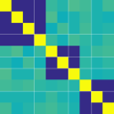
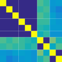
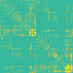
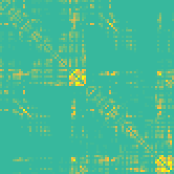
Figure 1: A motivating example based on synthetically generated data via the SimTB MATLAB toolbox [62, 4]. Fig. 1a shows the time profile of four brain-network resting states (ten nodes). For each state, the functional connectivity pattern stays fixed (Figs. 1b1e). Fig. 1f demonstrates a single realization of a single-node BOLD time series. Average covariance (Figs. 1g1j) and partial-correlation (PC) (Figs. 1k1n) matrices are obtained by sample averaging 100100100 realizations of the covariance and PC matrices, computed from the BOLD time series whose length equals the time span of a network state. No sample averaging is considered in the computation of the PC matrices of Figs. 1o1r.

To motivate the following discussion, consider the ten-node resting-state brain-network (RSBN) toy example of Fig. 1, with four distinct network states/structures whose evolution over time is shown in Fig. 1a. Those states are associated with the four functional connectivity matrices of Figs. 1b1e: nodes of the same color are considered to be connected, while no connection is established among nodes with different colors. For each state, connectivity matrices stay fixed. Based on the previous connectivity matrices, blood-oxygen-level dependent (BOLD) time series [51], e.g., Fig. 1f, are simulated via the SimTB MATLAB toolbox [62, 4], under a generation mechanism detailed in Sec. V-A. Examples of features extracted from the BOLD time series are the covariance (Figs. 1g1j) and partial-correlation matrices (Figs. 1k1n), computed via correlations of the time series whose time spans are set equal to the time span of a single state; see Sec. III for a detailed description. For patterns to emerge, Figs. 1g1n suggest that sample averaging of features over many time-series realizations is needed. On the contrary, Figs. 1o1r demonstrate that partial-correlation matrices, obtained without any sample averaging, do not offer much help in identifying the latent connectivity structure. Since multiple realizations of BOLD time series are hard to find in practice, rather than associating a single feature with a network state (Figs. 1o1r), it would be preferable to extract a sequence of features (xt)tsubscriptsubscript𝑥𝑡𝑡(x_{t})_{t} (t𝑡t denotes discrete time), e.g., running averages of covariance matrices, to characterize a network state. This is also in accordance with recent evidence showing that brain-network resting states demonstrate dynamic attributes, e.g., [15]. Indeed, the usual presupposition that functional connectivity is static over relatively large period of times has been challenged in works focusing on time-varying connectivity patterns [60, 4, 85, 47, 13], shifting the fMRI/EEG paradigm to the so-called “chronnectome” setting, where coupling within the brain network is dynamic, and two or more brain regions or sets of regions, all possibly evolving in time, are coupled with connective strengths that are also themselves explicit functions of time [17]. Such an approach has been already utilized to show that sleep states can be predicted via connectivity patterns at given times [72], and that schizophrenia can be correctly identified [22].

The previous discussion brings forth the following pressing questions: (i) Are there features that carve the latent network state/structure out of the observed network-wide time series? Is it possible to extract a sequence of features from a time series to capture a possibly dynamically evolving network state, as Fig. 1 and the related discussion suggest? (ii) Is there any model that injects geometrical arguments in the feature space, and is there any way to exploit that geometry to design a learning (in particular clustering) algorithm which provides state-of-the-art performance?

I-A Contributions of this work

This paper provides answers to the previous questions. Although the advocated methods, together with the underlying theory, apply to any network-wide time series, this paper focuses on brain-networks. Time-series data are processed sequentially via a finite-size sliding window that moves along the time axis to extract features which monitor the possibly time-varying state/structure of the network (Fig. 2b; Secs. II and III). Two feature-extraction schemes, novel in exploiting latent Riemannian geometry within network-wide time series, are introduced.

First, motivated by Granger-causality arguments, which play a prominent role in time-series analysis [31, 21, 26, 11], an auto-regressive moving average model is proposed to extract low-rank linear vector subspaces from the columns of appropriately defined observability matrices. Such linear subspaces demonstrate a remarkable geometrical property: they are points of the Grassmannian, a well-known Riemannian manifold (Sec. II).

Second, Sec. III generalizes the popular network-analytic tool of “linear” partial correlations (PCs) [39] to “non-linear” PCs, via reproducing kernel functions (cf. Appendix A), to capture the likely non-linear dependencies among network nodes, e.g., [38]. Geometry is also prominent in Sec. III: Prop. 1 demonstrates that matrices generated by kernel-based PCs are points of the celebrated Riemannian manifold of positive-definite matrices.

Capitalizing on the Riemannian-geometry thread that binds the previous feature-extraction schemes, learning, in particular clustering, is performed in a Riemannian manifold \mathpzc{M}. The key hypothesis, adopted from the very recent [79, 80], is the Riemannian multi-manifold modeling (RMMM) assumption: each cluster constitutes a submanifold of \mathpzc{M}, and distinguishing disparate time series amounts to clustering multiple Riemannian submanifolds; cf. Figs. 2b and 3a. This is in contrast with the prevailing perception of clusters in literature as “well-concentrated” data clouds, whose convex hulls can be (approximately) separated by hyperplanes in the feature space, a hypothesis which lies also beneath the success of Kmeans and variants [73]. In contrast, RMMM, as well as the advocated clustering algorithm of Sec. IV, allow for clusters (submanifolds) to intersect. The extensive numerical tests of Sec. V demonstrate that the proposed framework outperforms classical and state-of-the-art techniques in clustering brain-network states/structures.

I-B Prior art

Although the majority of methods on time-series clustering follows the “shape-based” approach, where clustering is applied to raw time-series data [2], fewer studies have focused on model/feature-based approaches, such as the present one [2, Table 4]. Study [37] fits an auto-regressive integrated moving average (ARIMA) model to non-network-wide time-series data, measures dissimilarities of patterns via the (Euclidean) 2subscript2\ell_{2}-distance of cepstrum coefficients, and applies the Kmedoids algorithm to cluster cepstum-coefficient patterns. In [28], fuzzy Cmeans is applied to vectors comprising the Pearson’s correlation coefficients of fMRI time series, under the 2subscript2\ell_{2}- and a hyperbolic-distance metric. In [53], hierarchical clustering is applied to functional connectivity matrices, comprising Pearson’s correlation coefficients of BOLD time series via the 2subscript2\ell_{2}-distance. Once again, the 2subscript2\ell_{2}-distance is used in [41], together with Kmeans and its sparsity-cognizant K-SVD variant, in clustering functional connectivity matrices which are formed by Pearson’s correlation coefficients, as well as low-rank matrices obtained via PCA. In [4], Kmeans is applied to windowed correlation matrices, under both the 1subscript1\ell_{1}- and 2subscript2\ell_{2}-distances. Kmeans is also used in clustering brain electrical activity into microstates in [56].

In all of the previous cases, Kmeans and variants are predicated on the assumption that a “cluster center” represents well the “spread” or variability of the data-cloud associated with each cluster. Moreover, any underlying feature-space Riemannian geometry is not exploited. This is in contrast with the RMMM hypothesis, advocated by this paper, where clusters are modeled as Riemannian submanifolds, allowed to intersect and to have a “spread” which cannot be captured by a single cluster-center point. To highlight such a difference, Kmeans under the standard 2subscript2\ell_{2}-distance will be employed in all tests in Sec. V. An application of the Riemannian (Grassmann) distance between low-rank matrices to detect network-state transitions in fMRI time series can be found in [46]. However, Grassmmanian geometry is exploited only up to the use of the distance metric in [46], without taking advantage of the rich first-order (tangential) information of submanifolds, as the current study offers in Sec. IV. Another line of fruitful research focuses on detecting communities within brain networks (e.g., [54]) by utilizing powerful concepts drawn from network/graph theory, such as modularity [50]. Due to lack of space, such a community-detection route is not pursued in this paper, and the related discussion is deferred to a future publication.

Regarding manifold clustering, most of the algorithms stem from schemes developed originally for Euclidean spaces. An extension of Kmeans to Grassmannians, with an application to non-negative matrix factorization, was presented in [34]. The mean-shift algorithm was also generalized to analytic manifolds in [71, 18]. Geodesic distances of product manifolds were utilized for clustering human expressions, gestures, and actions in video sequences in [52]. Moreover, spectral clustering and nonlinear dimensionality reduction techniques were extended to Riemannian manifolds in [27]. Such schemes are quite successful when the convex hulls of clusters are well-separated; however, they often fail when clusters intersect or are closely located. Clustering data-sets which demonstrate low-dimensional structure is recently accommodated by unions of affine subspaces or submanifold models. Submanifolds are usually restricted to manifolds embedded in either a Euclidean space or the sphere. Unions of affine subspace models, a.k.a. hybrid linear modeling (HLM) or subspace clustering, have been recently attracting growing interest, e.g., [77, 20, 42, 67]. There are fewer strategies for the union of submanifolds model, a.k.a. manifold clustering [5, 6, 29, 30, 40, 81, 24, 19, 68, 36]. Notwithstanding, only higher-order spectral clustering and spectral local PCA are theoretically guaranteed [5, 6]. Multiscale strategies for data on Riemannian manifolds were reported in [57]. The following discussion is based on [79, 80], where tangent spaces and angular information of submanifolds are utilized in a novel way. Even of a different context, the basic principles of [57] share common ground with those in [79, 80]. It is worth noting that a simplified version of the algorithm in Sec. IV offers theoretical guarantees. This paper attempts, for the first time in the network-science literature, to exploit the first-order (tangential) information of Riemannian submanifolds in clustering dynamic time series.

I-C Notation

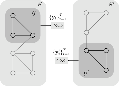
Having \mathbb{R} and \mathbb{Z} stand for the set of all real and integer numbers, respectively, let >0:=(0,+)assignsubscriptabsent00\mathbb{R}_{>0}:=(0,+\infty) and >0:={1,2,}{0,1,2,}=:0\mathbb{Z}_{>0}:=\{1,2,\ldots\}\subset\{0,1,2,\ldots\}=:\mathbb{Z}_{\geq 0}. Column vectors and matrices are denoted by upright boldfaced symbols, e.g., 𝐲𝐲\mathbf{y}, while row vectors are denoted by slanted boldfaced ones, e.g., 𝒚𝒚\bm{y}. Vector/matrix transposition is denoted by the superscript top\top. Notation 𝐀()𝟎succeeds𝐀succeeds-or-equals0\mathbf{A}\!\!\succ\!\!(\succeq)\mathbf{0} characterizes a symmetric positive (semi)definite [P(S)D] matrix. Consider a (brain) network/graph 𝒢:=(𝒩,)assign𝒢𝒩\mathscr{G}:=(\mathscr{N},\mathscr{E}), with sets of nodes 𝒩𝒩\mathscr{N} and edges \mathscr{E}. In the case of fMRI data, nodes could be defined as (contiguous) voxels belonging to either anatomically defined or data-driven regions [58]. Each node ν𝒩𝜈𝒩\nu\in\mathscr{N} is annotated by a real-valued random variable (r.v.) Yνsubscript𝑌𝜈Y_{\nu}, whose realizations comprise the time series associated with the ν𝜈\nuth node. Consider a subgraph 𝒢=(𝒱,)𝒢𝒱\mathpzc{G}=(\mathpzc{V},\mathpzc{E}) of 𝒢𝒢\mathscr{G}, with cardinality N𝒢:=|𝒱|assignsubscript𝑁𝒢𝒱N_{\mathpzc{G}}:=\lvert\mathpzc{V}\rvert, e.g., (i) 𝒢=𝒢𝒢𝒢\mathpzc{G}=\mathscr{G}; and (ii) 𝒢𝒢\mathpzc{G}is a singleton 𝒢={ν}𝒢𝜈\mathpzc{G}=\{\nu\}, for some node ν𝜈\nu. Realizations {yνt}ν𝒱subscriptsubscript𝑦𝜈𝑡𝜈𝒱\{y_{\nu t}\}_{\nu\in\mathpzc{V}}, or, a snapshot of 𝒢𝒢\mathpzc{G} at the t𝑡tth time instance, are collected into the N𝒢×1subscript𝑁𝒢1N_{\mathpzc{G}}\times 1 vector 𝐲tsubscript𝐲𝑡\mathbf{y}_{t}, and form the N𝒢×Tsubscript𝑁𝒢𝑇N_{\mathpzc{G}}\times T matrix 𝐘:=[𝐲1,,𝐲T]assign𝐘subscript𝐲1subscript𝐲𝑇\mathbf{Y}:=[\mathbf{y}_{1},\ldots,\mathbf{y}_{T}] over the time span t{1,,T}𝑡1𝑇t\in\{1,\ldots,T\}; cf. Fig. 2. For subgraph 𝒢𝒢\mathpzc{G}, and a τw>0subscript𝜏wsubscriptabsent0\tau_{\text{w}}\in\mathbb{Z}_{>0}, which represents the length of a “sliding window” that moves forward along the time axis, snapshots (𝐲τ)τ=tt+τw1superscriptsubscriptsubscript𝐲𝜏𝜏𝑡𝑡subscript𝜏w1(\mathbf{y}_{\tau})_{\tau=t}^{t+\tau_{\text{w}}-1} of 𝒢𝒢\mathpzc{G} are gathered into the data matrix 𝐘t:=[𝐲t,𝐲t+1,,𝐲t+τw1]assignsubscript𝐘𝑡subscript𝐲𝑡subscript𝐲𝑡1subscript𝐲𝑡subscript𝜏w1\mathbf{Y}_{t}:=[\mathbf{y}_{t},\mathbf{y}_{t+1},\ldots,\mathbf{y}_{t+\tau_{\text{w}}-1}]; cf. Fig. 2b. The following two sections introduce two ways to capture intra-network connectivity patterns and dynamics.
Refer to caption
(a) Network-wide time series
Refer to caption
(b) Flowchart of the feature-extraction scheme
Figure 2: (a) Subgraphs 𝒢𝒢\mathpzc{G} and 𝒢superscript𝒢\mathpzc{G}^{\prime} of the potentially different graphs 𝒢𝒢\mathscr{G} and 𝒢superscript𝒢\mathscr{G}^{\prime}, respectively. Node ν𝜈\nu of 𝒢𝒢\mathpzc{G} emanates signal yνtsubscript𝑦𝜈𝑡y_{\nu t} (realization of a stochastic process) at discrete time t𝑡t. All those values are gathered in the N𝒢×1subscript𝑁𝒢1N_{\mathpzc{G}}\times 1 vector 𝐲tsubscript𝐲𝑡\mathbf{y}_{t} (snapshot of 𝒢𝒢\mathpzc{G} at time t𝑡t). Such snapshots, observed over the time span t{1,2,,T}𝑡12𝑇t\in\{1,2,\ldots,T\}, are collected into matrices 𝐘:=[𝐲1,,𝐲T]assign𝐘subscript𝐲1subscript𝐲𝑇\mathbf{Y}:=[\mathbf{y}_{1},\ldots,\mathbf{y}_{T}] and 𝐘:=[𝐲1,,𝐲T]assignsuperscript𝐘superscriptsubscript𝐲1superscriptsubscript𝐲𝑇\mathbf{Y}^{\prime}:=[\mathbf{y}_{1}^{\prime},\ldots,\mathbf{y}_{T}^{\prime}]. The goal is to distinguish 𝒢𝒢\mathpzc{G} and 𝒢superscript𝒢\mathpzc{G}^{\prime} from the time-series information included in 𝐘𝐘\mathbf{Y} and 𝐘superscript𝐘\mathbf{Y}^{\prime}. (b) A sliding window sequentially collects data (𝐘t:=[𝐲t,𝐲t+1,,𝐲t+τw1])tsubscriptassignsubscript𝐘𝑡subscript𝐲𝑡subscript𝐲𝑡1subscript𝐲𝑡subscript𝜏w1𝑡(\mathbf{Y}_{t}:=[\mathbf{y}_{t},\mathbf{y}_{t+1},\ldots,\mathbf{y}_{t+\tau_{\text{w}}-1}])_{t} and extracts features (Secs. II and III) which can be viewed as points on or close to a Riemannian submanifold (the Riemannian multi-manifold modeling hypothesis (RMMM) [79, 80]).

II ARMA Modeling

Motivated by Granger causality [31, 21, 26, 11], this section provides a scheme for capturing spatio-temporal dependencies among network nodes. Granger causality is built on a linear auto-regressive (AR) model that approximates 𝐲tsubscript𝐲𝑡\mathbf{y}_{t} by a linear combination of the copies {𝐲tj}j=1psuperscriptsubscriptsubscript𝐲𝑡𝑗𝑗1𝑝\{\mathbf{y}_{t-j}\}_{j=1}^{p}: 𝐲t:=j=1p𝐃j𝐲tj+𝐯tassignsubscript𝐲𝑡superscriptsubscript𝑗1𝑝subscript𝐃𝑗subscript𝐲𝑡𝑗subscript𝐯𝑡\mathbf{y}_{t}:=\sum_{j=1}^{p}\mathbf{D}_{j}\mathbf{y}_{t-j}+\mathbf{v}_{t}, for some N𝒢×N𝒢subscript𝑁𝒢subscript𝑁𝒢N_{\mathpzc{G}}\times N_{\mathpzc{G}} matrices {𝐃j}j=1psuperscriptsubscriptsubscript𝐃𝑗𝑗1𝑝\{\mathbf{D}_{j}\}_{j=1}^{p}, p>0𝑝subscriptabsent0p\in\mathbb{Z}_{>0}, and 𝐯tsubscript𝐯𝑡\mathbf{v}_{t} is the r.v. that quantifies noise and modeling inaccuracies. High-quality estimates of the pN𝒢2𝑝superscriptsubscript𝑁𝒢2pN_{\mathpzc{G}}^{2} entries of {𝐃j}j=1psuperscriptsubscriptsubscript𝐃𝑗𝑗1𝑝\{\mathbf{D}_{j}\}_{j=1}^{p} require a large number of training data, and thus an abundance of computational resources, especially in cases of large-scale networks. The following discussion provides a way to reduce the number of unknowns in the previous identification task by capitalizing on the low-rank arguments of the more general (linear) auto-regressive moving average (ARMA) model.

ARMA models are powerful parametric tools for spatio-temporal series analysis with numerous applications in signal processing, controls and machine learning [43, 1, 75]. ARMA modeling describes 𝐲τsubscript𝐲𝜏\mathbf{y}_{\tau} via the ρ×1(ρN𝒢)𝜌1much-less-than𝜌subscript𝑁𝒢\rho\times 1\ (\rho\ll N_{\mathpzc{G}}) latent vector 𝐳τsubscript𝐳𝜏\mathbf{z}_{\tau} [43, §10.6, p. 340]:

𝐳τsubscript𝐳𝜏\displaystyle\mathbf{z}_{\tau} =j=1p𝐀j𝐳τj+𝐰τ,absentsuperscriptsubscript𝑗1𝑝subscript𝐀𝑗subscript𝐳𝜏𝑗subscript𝐰𝜏\displaystyle=\sum\nolimits_{j=1}^{p}\mathbf{A}_{j}\mathbf{z}_{\tau-j}+\mathbf{w}_{\tau}\,, (1a)
𝐲τsubscript𝐲𝜏\displaystyle\mathbf{y}_{\tau} =𝐂𝐳τ+𝐯τ,absentsubscript𝐂𝐳𝜏subscript𝐯𝜏\displaystyle=\mathbf{C}\mathbf{z}_{\tau}+\mathbf{v}_{\tau}\,, (1b)

where (i) (1a) is called the state and (1b) the space equation; (ii) ρ𝜌\rhois the order of the model; (iii) 𝐂N𝒢×ρ𝐂superscriptsubscript𝑁𝒢𝜌\mathbf{C}\in\mathbb{R}^{N_{\mathpzc{G}}\times\rho}is the observation and {𝐀j}j=1pρ×ρsuperscriptsubscriptsubscript𝐀𝑗𝑗1𝑝superscript𝜌𝜌\{\mathbf{A}_{j}\}_{j=1}^{p}\subset\mathbb{R}^{\rho\times\rho} the transition matrices; and (iv) 𝐯τsubscript𝐯𝜏\mathbf{v}_{\tau}as well as 𝐰τsubscript𝐰𝜏\mathbf{w}_{\tau} are realizations of zero-mean, white-noise random processes, uncorrelated both w.r.t. each other and 𝐲τsubscript𝐲𝜏\mathbf{y}_{\tau}. As in AR modeling, matrices {𝐀j}j=1psuperscriptsubscriptsubscript𝐀𝑗𝑗1𝑝\{\mathbf{A}_{j}\}_{j=1}^{p} manifest causality throughout the process {𝐳t}subscript𝐳𝑡\{\mathbf{z}_{t}\}. The system identification problem (1) requires estimation of the N𝒢ρ+pρ2subscript𝑁𝒢𝜌𝑝superscript𝜌2N_{\mathpzc{G}}\rho+p\rho^{2} entries of 𝐂𝐂\mathbf{C} and {𝐀j}j=1psuperscriptsubscriptsubscript𝐀𝑗𝑗1𝑝\{\mathbf{A}_{j}\}_{j=1}^{p}, which are many less than the pN𝒢2𝑝superscriptsubscript𝑁𝒢2pN_{\mathpzc{G}}^{2} ones in the AR modeling case, provided that ρN𝒢much-less-than𝜌subscript𝑁𝒢\rho\ll N_{\mathpzc{G}}. For example, any 0<ϖ[(1+4p2)1/21]/(2p)0italic-ϖdelimited-[]superscript14superscript𝑝21212𝑝0<\varpi\leq[(1+4p^{2})^{1/2}-1]/(2p) guarantees that for ρ:=ϖN𝒢assign𝜌italic-ϖsubscript𝑁𝒢\rho:=\varpi N_{\mathpzc{G}}, N𝒢ρ+pρ2pN𝒢2subscript𝑁𝒢𝜌𝑝superscript𝜌2𝑝superscriptsubscript𝑁𝒢2N_{\mathpzc{G}}\rho+p\rho^{2}\leq pN_{\mathpzc{G}}^{2}.

To simplify (1), re-define 𝐳τsubscript𝐳𝜏\mathbf{z}_{\tau} and 𝐰τsubscript𝐰𝜏\mathbf{w}_{\tau} as the pρ×1𝑝𝜌1p\rho\times 1 vectors [𝐳τ,𝐳τ1,,𝐳τp+1]superscriptsuperscriptsubscript𝐳𝜏topsuperscriptsubscript𝐳𝜏1topsuperscriptsubscript𝐳𝜏𝑝1toptop[\mathbf{z}_{\tau}^{\top},\mathbf{z}_{\tau-1}^{\top},\ldots,\mathbf{z}_{\tau-p+1}^{\top}]^{\top} and [𝐰τ,𝟎,,𝟎]superscriptsuperscriptsubscript𝐰𝜏topsuperscript0topsuperscript0toptop[\mathbf{w}_{\tau}^{\top},\mathbf{0}^{\top},\ldots,\mathbf{0}^{\top}]^{\top}, respectively. Then, it can be easily verified that there exist a pρ×pρ𝑝𝜌𝑝𝜌p\rho\times p\rho matrix 𝐀0subscript𝐀0\mathbf{A}_{0} and an N𝒢×pρsubscript𝑁𝒢𝑝𝜌N_{\mathpzc{G}}\times p\rho matrix 𝐂0subscript𝐂0\mathbf{C}_{0} such that (1) is recast as

𝐳τ=𝐀0𝐳τ1+𝐰τ,𝐲τ=𝐂0𝐳τ+𝐯τ.formulae-sequencesubscript𝐳𝜏subscript𝐀0subscript𝐳𝜏1subscript𝐰𝜏subscript𝐲𝜏subscript𝐂0subscript𝐳𝜏subscript𝐯𝜏\displaystyle\mathbf{z}_{\tau}=\mathbf{A}_{0}\mathbf{z}_{\tau-1}+\mathbf{w}_{\tau}\,,\qquad\mathbf{y}_{\tau}=\mathbf{C}_{0}\mathbf{z}_{\tau}+\mathbf{v}_{\tau}\,. (2)

Further, it can be verified by (2) that for any i0𝑖subscriptabsent0i\in\mathbb{Z}_{\geq 0},

𝐲t+i=𝐂0𝐀0i𝐳t+j=1i𝐂0𝐀0ij𝐰t+j+𝐯t+i,subscript𝐲𝑡𝑖subscript𝐂0superscriptsubscript𝐀0𝑖subscript𝐳𝑡superscriptsubscript𝑗1𝑖subscript𝐂0superscriptsubscript𝐀0𝑖𝑗subscript𝐰𝑡𝑗subscript𝐯𝑡𝑖\displaystyle\mathbf{y}_{t+i}=\mathbf{C}_{0}\mathbf{A}_{0}^{i}\mathbf{z}_{t}+\sum\nolimits_{j=1}^{i}\mathbf{C}_{0}\mathbf{A}_{0}^{i-j}\mathbf{w}_{t+j}+\mathbf{v}_{t+i}\,,

where 𝐀00:=𝐈pρassignsuperscriptsubscript𝐀00subscript𝐈𝑝𝜌\mathbf{A}_{0}^{0}:=\mathbf{I}_{p\rho} and j=10𝐂0𝐀0j𝐰t+j:=𝟎assignsuperscriptsubscript𝑗10subscript𝐂0superscriptsubscript𝐀0𝑗subscript𝐰𝑡𝑗0\sum\nolimits_{j=1}^{0}\mathbf{C}_{0}\mathbf{A}_{0}^{-j}\mathbf{w}_{t+j}:=\mathbf{0}. Fix now an m>0𝑚subscriptabsent0m\in\mathbb{Z}_{>0} and define the mN𝒢×1𝑚subscript𝑁𝒢1mN_{\mathpzc{G}}\times 1 vector

𝐲fτ:=[𝐲τ,𝐲τ+1,𝐲τ+m1],assignsubscript𝐲f𝜏superscriptsuperscriptsubscript𝐲𝜏topsuperscriptsubscript𝐲𝜏1topsuperscriptsubscript𝐲𝜏𝑚1toptop\displaystyle\bm{\mathcalboondox{y}}_{\text{f}\tau}:=[\mathbf{y}_{\tau}^{\top},\mathbf{y}_{\tau+1}^{\top}\ldots,\mathbf{y}_{\tau+m-1}^{\top}]^{\top}\,, (3)

where sub-script f stresses the fact that one moves forward in time and utilizes data {𝐲τ}τ=ττ+m1superscriptsubscriptsubscript𝐲superscript𝜏superscript𝜏𝜏𝜏𝑚1\{\mathbf{y}_{\tau^{\prime}}\}_{\tau^{\prime}=\tau}^{\tau+m-1} to define 𝐲fτsubscript𝐲f𝜏\bm{\mathcalboondox{y}}_{\text{f}\tau}. It can be verified that 𝐲fτ=𝐎(m)𝐳τ+𝐞fτsubscript𝐲f𝜏superscript𝐎𝑚subscript𝐳𝜏subscript𝐞f𝜏\bm{\mathcalboondox{y}}_{\text{f}\tau}=\mathbf{O}^{(m)}\mathbf{z}_{\tau}+\bm{\mathcalboondox{e}}_{\text{f}\tau}, where 𝐎(m)superscript𝐎𝑚\mathbf{O}^{(m)} is the m𝑚mth-order observability matrix of size mN𝒢×pρ𝑚subscript𝑁𝒢𝑝𝜌mN_{\mathpzc{G}}\times p\rho: 𝐎(m):=[𝐂0,(𝐂0𝐀0),,(𝐂0𝐀0m1)]assignsuperscript𝐎𝑚superscriptsuperscriptsubscript𝐂0topsuperscriptsubscript𝐂0subscript𝐀0topsuperscriptsubscript𝐂0superscriptsubscript𝐀0𝑚1toptop\mathbf{O}^{(m)}:=[\mathbf{C}_{0}^{\top},(\mathbf{C}_{0}\mathbf{A}_{0})^{\top},\ldots,(\mathbf{C}_{0}\mathbf{A}_{0}^{m-1})^{\top}]^{\top}, and 𝐞fτsubscript𝐞f𝜏\bm{\mathcalboondox{e}}_{\text{f}\tau} is defined as the vector whose entries from iN𝒢+1𝑖subscript𝑁𝒢1iN_{\mathpzc{G}}+1 till (i+1)N𝒢𝑖1subscript𝑁𝒢(i+1)N_{\mathpzc{G}}, for i{0,,m1}𝑖0𝑚1i\in\{0,\ldots,m-1\}, are given by j=1i𝐂0𝐀0ij𝐰t+j+𝐯t+isuperscriptsubscript𝑗1𝑖subscript𝐂0superscriptsubscript𝐀0𝑖𝑗subscript𝐰𝑡𝑗subscript𝐯𝑡𝑖\sum\nolimits_{j=1}^{i}\mathbf{C}_{0}\mathbf{A}_{0}^{i-j}\mathbf{w}_{t+j}+\mathbf{v}_{t+i}. Since 𝐞fτsubscript𝐞f𝜏\bm{\mathcalboondox{e}}_{\text{f}\tau} contains zero-mean noise terms, it can be also verified that the conditional expectation of 𝐲fτsubscript𝐲f𝜏\bm{\mathcalboondox{y}}_{\text{f}\tau} given 𝐳τsubscript𝐳𝜏\mathbf{z}_{\tau} is 𝔼{𝐲fτ\nonscript|\nonscript𝐳τ}=𝐎(m)𝐳τ𝔼conditionalsubscript𝐲f𝜏\nonscript\nonscriptsubscript𝐳𝜏superscript𝐎𝑚subscript𝐳𝜏\operatorname{\mathbb{E}}\{\bm{\mathcalboondox{y}}_{\text{f}\tau}\nonscript\,|\allowbreak\nonscript\,\mathopen{}\mathbf{z}_{\tau}\}=\mathbf{O}^{(m)}\mathbf{z}_{\tau}.

It is well-known that any change of basis 𝐳~τ:=𝐏1𝐳τassignsubscript~𝐳𝜏superscript𝐏1subscript𝐳𝜏\tilde{\mathbf{z}}_{\tau}:=\mathbf{P}^{-1}\mathbf{z}_{\tau} in the state space, where 𝐏𝐏\mathbf{P} is non-singular, renders

𝐳~τ=𝐏1𝐀0𝐏𝐳~τ1+𝐰~τ,𝐲τ=𝐂0𝐏𝐳~τ+𝐯τ,formulae-sequencesubscript~𝐳𝜏superscript𝐏1subscript𝐀0𝐏subscript~𝐳𝜏1subscript~𝐰𝜏subscript𝐲𝜏subscript𝐂0𝐏subscript~𝐳𝜏subscript𝐯𝜏\displaystyle\tilde{\mathbf{z}}_{\tau}=\mathbf{P}^{-1}\mathbf{A}_{0}\mathbf{P}\tilde{\mathbf{z}}_{\tau-1}+\tilde{\mathbf{w}}_{\tau}\,,\qquad\mathbf{y}_{\tau}=\mathbf{C}_{0}\mathbf{P}\tilde{\mathbf{z}}_{\tau}+\mathbf{v}_{\tau}\,, (4)

with observation and transition matrices 𝐂~0:=𝐂0𝐏assignsubscript~𝐂0subscript𝐂0𝐏\tilde{\mathbf{C}}_{0}:=\mathbf{C}_{0}\mathbf{P} and 𝐀~0:=𝐏1𝐀0𝐏assignsubscript~𝐀0superscript𝐏1subscript𝐀0𝐏\tilde{\mathbf{A}}_{0}:=\mathbf{P}^{-1}\mathbf{A}_{0}\mathbf{P}, respectively, equivalent to (2) in the sense of describing the same signal 𝐲τsubscript𝐲𝜏\mathbf{y}_{\tau} [43, §10.6]. The observability matrix of (4) satisfies 𝐎~(m)=𝐎(m)𝐏superscript~𝐎𝑚superscript𝐎𝑚𝐏\tilde{\mathbf{O}}^{(m)}=\mathbf{O}^{(m)}\mathbf{P}. Remarkably, due to the non-singularity of 𝐏𝐏\mathbf{P}, even if 𝐎~(m)𝐎(m)superscript~𝐎𝑚superscript𝐎𝑚\tilde{\mathbf{O}}^{(m)}\neq\mathbf{O}^{(m)}, their columns span the same linear subspace.

Given the previous ambiguity of ARMA modeling w.r.t. 𝐏𝐏\mathbf{P}, to extract features that uniquely characterize (2), it is preferable to record the column space of 𝐎(m)superscript𝐎𝑚\mathbf{O}^{(m)}, instead of 𝐎(m)superscript𝐎𝑚\mathbf{O}^{(m)} itself. To this end, notice that for small values of pρ𝑝𝜌p\rho, it is often the case in practice to have mN𝒢pρmuch-greater-than𝑚subscript𝑁𝒢𝑝𝜌mN_{\mathpzc{G}}\gg p\rho, which renders the “tall” 𝐎(m)superscript𝐎𝑚\mathbf{O}^{(m)} full-column rank, with high probability. The “column space” of 𝐎(m)superscript𝐎𝑚\mathbf{O}^{(m)} becomes a (pρ)𝑝𝜌(p\rho)-dimensional linear subspace of mN𝒢superscript𝑚subscript𝑁𝒢\mathbb{R}^{mN_{\mathpzc{G}}}, or equivalently, a point in the Grassmannian Gr(mN𝒢,pρ):={\text{Gr}(mN_{\mathpzc{G}},p\rho):=\{all (pρ)𝑝𝜌(p\rho)-rank linear subspaces of mN𝒢}\mathbb{R}^{mN_{\mathpzc{G}}}\}. Apparently, Gr(mN𝒢,pρ)Gr𝑚subscript𝑁𝒢𝑝𝜌\text{Gr}(mN_{\mathpzc{G}},p\rho) is a (smooth) Riemannian manifold of dimension pρ(mN𝒢pρ)𝑝𝜌𝑚subscript𝑁𝒢𝑝𝜌p\rho(mN_{\mathpzc{G}}-p\rho) [23, 74]. The Grassmannian formulation removes the previous 𝐏𝐏\mathbf{P}-similarity-transform ambiguity in (4): since any linear subspace possesses an orthonormal basis, it can be easily verified that Gr(mN𝒢,pρ)={[𝐔]\nonscript|\nonscript𝐔mN𝒢×pρ;𝐔𝐔=𝐈pρ}Gr𝑚subscript𝑁𝒢𝑝𝜌conditional-setdelimited-[]𝐔\nonscriptformulae-sequence\nonscript𝐔superscript𝑚subscript𝑁𝒢𝑝𝜌superscript𝐔top𝐔subscript𝐈𝑝𝜌\text{Gr}(mN_{\mathpzc{G}},p\rho)=\{[\mathbf{U}]\nonscript\,|\allowbreak\nonscript\,\mathopen{}\mathbf{U}\in\mathbb{R}^{mN_{\mathpzc{G}}\times p\rho};\mathbf{U}^{\top}\mathbf{U}=\mathbf{I}_{p\rho}\}, where given the orthogonal 𝐔𝐔\mathbf{U}, point [𝐔]Gr(mN𝒢,pρ)delimited-[]𝐔Gr𝑚subscript𝑁𝒢𝑝𝜌[\mathbf{U}]\in\text{Gr}(mN_{\mathpzc{G}},p\rho) stands for [𝐔]:={𝐔𝐏\nonscript|\nonscript𝐏pρ×pρis non-singular}assigndelimited-[]𝐔conditional-set𝐔𝐏\nonscript\nonscript𝐏superscript𝑝𝜌𝑝𝜌is non-singular[\mathbf{U}]:=\{\mathbf{UP}\nonscript\,|\allowbreak\nonscript\,\mathopen{}\mathbf{P}\in\mathbb{R}^{p\rho\times p\rho}\ \text{is non-singular}\}, i.e., [𝐔]delimited-[]𝐔[\mathbf{U}] gathers all bases for the column space of 𝐔𝐔\mathbf{U}.

Fix now a τf>0subscript𝜏fsubscriptabsent0\tau_{\text{f}}\in\mathbb{Z}_{>0} and define the mN𝒢×τf𝑚subscript𝑁𝒢subscript𝜏fmN_{\mathpzc{G}}\times\tau_{\text{f}} matrices

𝐘fτsubscript𝐘f𝜏\displaystyle\bm{\mathcalboondox{Y}}_{\text{f}\tau} :=[𝐲fτ,𝐲f,τ+1,,𝐲f,τ+τf1],assignabsentsubscript𝐲f𝜏subscript𝐲f𝜏1subscript𝐲f𝜏subscript𝜏f1\displaystyle:=[\bm{\mathcalboondox{y}}_{\text{f}\tau},\bm{\mathcalboondox{y}}_{\text{f},\tau+1},\ldots,\bm{\mathcalboondox{y}}_{\text{f},\tau+\tau_{\text{f}}-1}]\,, (5)
𝐄fτsubscript𝐄f𝜏\displaystyle\bm{\mathcalboondox{E}}_{\text{f}\tau} :=[𝐞fτ,𝐞f,τ+1,,𝐞f,τ+τf1],assignabsentsubscript𝐞f𝜏subscript𝐞f𝜏1subscript𝐞f𝜏subscript𝜏f1\displaystyle:=[\bm{\mathcalboondox{e}}_{\text{f}\tau},\bm{\mathcalboondox{e}}_{\text{f},\tau+1},\ldots,\bm{\mathcalboondox{e}}_{\text{f},\tau+\tau_{\text{f}}-1}]\,,

as well as the pρ×τf𝑝𝜌subscript𝜏fp\rho\times\tau_{\text{f}} matrix 𝐙τ:=[𝐳τ,,𝐳τ+τf1]assignsubscript𝐙𝜏subscript𝐳𝜏subscript𝐳𝜏subscript𝜏f1\mathbf{Z}_{\tau}:=[\mathbf{z}_{\tau},\ldots,\mathbf{z}_{\tau+\tau_{\text{f}}-1}]. Then,

𝐘fτ=𝐎(m)𝐙τ+𝐄fτ.subscript𝐘f𝜏superscript𝐎𝑚subscript𝐙𝜏subscript𝐄f𝜏\displaystyle\bm{\mathcalboondox{Y}}_{\text{f}\tau}=\mathbf{O}^{(m)}\mathbf{Z}_{\tau}+\bm{\mathcalboondox{E}}_{\text{f}\tau}\,. (6)

To obtain high-quality estimates of 𝐎(m)superscript𝐎𝑚\mathbf{O}^{(m)} from (6), choose a τb>0subscript𝜏bsubscriptabsent0\tau_{\text{b}}\in\mathbb{Z}_{>0}, and define as in [43, §10.6] the τbN𝒢×1subscript𝜏bsubscript𝑁𝒢1\tau_{\text{b}}N_{\mathpzc{G}}\times 1 vector

𝐲bτ:=[𝐲τ,𝐲τ1,𝐲ττb+1],assignsubscript𝐲b𝜏superscriptsuperscriptsubscript𝐲𝜏topsuperscriptsubscript𝐲𝜏1topsuperscriptsubscript𝐲𝜏subscript𝜏b1toptop\displaystyle\bm{\mathcalboondox{y}}_{\text{b}\tau}:=\left[\mathbf{y}_{\tau}^{\top},\mathbf{y}_{\tau-1}^{\top}\ldots,\mathbf{y}_{\tau-\tau_{\text{b}}+1}^{\top}\right]^{\top}\,, (7a)
where, as opposed to (3), one moves τbsubscript𝜏b\tau_{\text{b}} steps backward in time to define 𝐲bτsubscript𝐲b𝜏\bm{\mathcalboondox{y}}_{\text{b}\tau}. Let also the τbN𝒢×τfsubscript𝜏bsubscript𝑁𝒢subscript𝜏f\tau_{\text{b}}N_{\mathpzc{G}}\times\tau_{\text{f}} matrix
𝐘bτ:=[𝐲bτ,𝐲b,τ+1,,𝐲b,τ+τf1].assignsubscript𝐘b𝜏subscript𝐲b𝜏subscript𝐲b𝜏1subscript𝐲b𝜏subscript𝜏f1\displaystyle\bm{\mathcalboondox{Y}}_{\text{b}\tau}:=[\bm{\mathcalboondox{y}}_{\text{b}\tau},\bm{\mathcalboondox{y}}_{\text{b},\tau+1},\ldots,\bm{\mathcalboondox{y}}_{\text{b},\tau+\tau_{\text{f}}-1}]\,. (7b)

By (6),

1τf𝐘f,t+τb𝐘b,t+τb11subscript𝜏fsubscript𝐘f𝑡subscript𝜏bsuperscriptsubscript𝐘b𝑡subscript𝜏b1top\displaystyle\tfrac{1}{\tau_{\text{f}}}\bm{\mathcalboondox{Y}}_{\text{f},t+\tau_{\text{b}}}\bm{\mathcalboondox{Y}}_{\text{b},t+\tau_{\text{b}}-1}^{\top}
=𝐎(m)1τf𝐙t+τb𝐘b,t+τb1+1τfτ=t+τbt+τb+τf1𝐞f,τ𝐲b,τ1.absentsuperscript𝐎𝑚1subscript𝜏fsubscript𝐙𝑡subscript𝜏bsuperscriptsubscript𝐘b𝑡subscript𝜏b1top1subscript𝜏fsubscriptsuperscript𝑡subscript𝜏bsubscript𝜏f1𝜏𝑡subscript𝜏bsubscript𝐞f𝜏superscriptsubscript𝐲b𝜏1top\displaystyle=\mathbf{O}^{(m)}\tfrac{1}{\tau_{\text{f}}}\mathbf{Z}_{t+\tau_{\text{b}}}\bm{\mathcalboondox{Y}}_{\text{b},t+\tau_{\text{b}}-1}^{\top}+\tfrac{1}{\tau_{\text{f}}}\smashoperator[]{\sum_{\tau=t+\tau_{\text{b}}}^{t+\tau_{\text{b}}+\tau_{\text{f}}-1}}\bm{\mathcalboondox{e}}_{\text{f},\tau}\bm{\mathcalboondox{y}}_{\text{b},\tau-1}^{\top}\,. (8)

To avoid any confusion regarding time indices, it is required that τwτf+τb+m1subscript𝜏wsubscript𝜏fsubscript𝜏b𝑚1\tau_{\text{w}}\geq\tau_{\text{f}}+\tau_{\text{b}}+m-1. Notice also that τ𝐞f,τ𝐲b,τ1subscript𝜏subscript𝐞f𝜏superscriptsubscript𝐲b𝜏1top\sum_{\tau}\bm{\mathcalboondox{e}}_{\text{f},\tau}\bm{\mathcalboondox{y}}_{\text{b},\tau-1}^{\top} comprises terms that result from the cross-correlations of 𝐲τsubscript𝐲𝜏\mathbf{y}_{\tau} with noise vectors 𝐰τsubscript𝐰superscript𝜏\mathbf{w}_{\tau^{\prime}} and 𝐯τ′′subscript𝐯superscript𝜏′′\mathbf{v}_{\tau^{\prime\prime}}, recorded at time instants τsuperscript𝜏\tau^{\prime} and τ′′superscript𝜏′′\tau^{\prime\prime} that lie ahead of τ𝜏\tau, and for which, according to the initial modeling assumptions, 𝐲τsubscript𝐲𝜏\mathbf{y}_{\tau} is uncorrelated with 𝐰τsubscript𝐰superscript𝜏\mathbf{w}_{\tau^{\prime}} and 𝐯τ′′subscript𝐯superscript𝜏′′\mathbf{v}_{\tau^{\prime\prime}}. If τfsubscript𝜏f\tau_{\text{f}} is set to be large, the law of large numbers suggests that the sample correlations in (1/τf)τ𝐞fτ𝐲b,τ11subscript𝜏fsubscript𝜏subscript𝐞f𝜏superscriptsubscript𝐲b𝜏1top(1/\tau_{\text{f}})\sum_{\tau}\bm{\mathcalboondox{e}}_{\text{f}\tau}\bm{\mathcalboondox{y}}_{\text{b},\tau-1}^{\top} approximate well the ensemble ones, which, as previously stated, are zero.

Motivated by (8), the estimation task of the observability matrix becomes as follows:

(𝐎^t(m),𝚷^t)argmin𝐎mN𝒢×pρ𝚷pρ×τbN𝒢1τf𝐘f,t+τb𝐘b,t+τb1𝐎𝚷F2.\displaystyle\left(\hat{\mathbf{O}}^{(m)}_{t},\hat{\bm{\Pi}}_{t}\right)\in\operatorname*{arg\,min}_{\begin{subarray}{c}\mathbf{O}\in\mathbb{R}^{mN_{\mathpzc{G}}\times p\rho}\\ \bm{\Pi}\in\mathbb{R}^{p\rho\times\tau_{\text{b}}N_{\mathpzc{G}}}\end{subarray}}\left\lVert\tfrac{1}{\tau_{\text{f}}}\bm{\mathcalboondox{Y}}_{\text{f},t+\tau_{\text{b}}}\bm{\mathcalboondox{Y}}_{\text{b},t+\tau_{\text{b}}-1}^{\top}-\mathbf{O}\bm{\Pi}\right\rVert_{\text{F}}^{2}\,. (9)

If r𝑟r denotes the rank of (1/τf)𝐘f,t+τb𝐘b,t+τb11subscript𝜏fsubscript𝐘f𝑡subscript𝜏bsuperscriptsubscript𝐘b𝑡subscript𝜏b1top({1}/{\tau_{\text{f}}})\bm{\mathcalboondox{Y}}_{\text{f},t+\tau_{\text{b}}}\bm{\mathcalboondox{Y}}_{\text{b},t+\tau_{\text{b}}-1}^{\top}, then its thin SVD is (1/τf)𝐘f,t+τb𝐘b,t+τb1=𝐔𝚺𝐕1subscript𝜏fsubscript𝐘f𝑡subscript𝜏bsuperscriptsubscript𝐘b𝑡subscript𝜏b1top𝐔𝚺superscript𝐕top({1}/{\tau_{\text{f}}})\bm{\mathcalboondox{Y}}_{\text{f},t+\tau_{\text{b}}}\bm{\mathcalboondox{Y}}_{\text{b},t+\tau_{\text{b}}-1}^{\top}=\mathbf{U}\bm{\Sigma}\mathbf{V}^{\top}, where 𝐔mN𝒢×r𝐔superscript𝑚subscript𝑁𝒢𝑟\mathbf{U}\in\mathbb{R}^{mN_{\mathpzc{G}}\times r} and 𝐕τbN𝒢×r𝐕superscriptsubscript𝜏bsubscript𝑁𝒢𝑟\mathbf{V}\in\mathbb{R}^{\tau_{\text{b}}N_{\mathpzc{G}}\times r} are orthogonal matrices, i.e., 𝐔𝐔=𝐈r=𝐕𝐕superscript𝐔top𝐔subscript𝐈𝑟superscript𝐕top𝐕\mathbf{U}^{\top}\mathbf{U}=\mathbf{I}_{r}=\mathbf{V}^{\top}\mathbf{V}, and 𝚺𝚺\bm{\Sigma} is the r×r𝑟𝑟r\times r diagonal matrix whose diagonal elements gather, in descending order, the non-zero singular values of (1/τf)𝐘f,t+τb𝐘b,t+τb11subscript𝜏fsubscript𝐘f𝑡subscript𝜏bsuperscriptsubscript𝐘b𝑡subscript𝜏b1top({1}/{\tau_{\text{f}}})\bm{\mathcalboondox{Y}}_{\text{f},t+\tau_{\text{b}}}\bm{\mathcalboondox{Y}}_{\text{b},t+\tau_{\text{b}}-1}^{\top}. Assuming that pρr𝑝𝜌𝑟p\rho\leq r, the celebrated Schmidt-Mirsky-Eckart-Young theorem [10] suggests that a solution to (9) is given by 𝐎^t(m)=𝐔:,1:pρsubscriptsuperscript^𝐎𝑚𝑡subscript𝐔::1𝑝𝜌\hat{\mathbf{O}}^{(m)}_{t}=\mathbf{U}_{:,1:p\rho}, where 𝐔:,1:pρsubscript𝐔::1𝑝𝜌\mathbf{U}_{:,1:p\rho} gathers the first pρ𝑝𝜌p\rho columns of 𝐔𝐔\mathbf{U}, and 𝚷^t=𝚺1:pρ,1:pρ𝐕:,1:pρsubscript^𝚷𝑡subscript𝚺:1𝑝𝜌1:𝑝𝜌subscriptsuperscript𝐕top::1𝑝𝜌\hat{\bm{\Pi}}_{t}=\bm{\Sigma}_{1:p\rho,1:p\rho}\mathbf{V}^{\top}_{:,1:p\rho}. The previous procedure of extracting a sequence of features {xt:=[𝐎^t(m)]}tsubscriptassignsubscript𝑥𝑡delimited-[]subscriptsuperscript^𝐎𝑚𝑡𝑡\{x_{t}:=[\hat{\mathbf{O}}^{(m)}_{t}]\}_{t} in the Grassmannian Gr(mN𝒢,pρ)Gr𝑚subscript𝑁𝒢𝑝𝜌\text{Gr}(mN_{\mathpzc{G}},p\rho) is summarized in Alg. 1. The dependence of the estimate 𝐎^t(m)subscriptsuperscript^𝐎𝑚𝑡\hat{\mathbf{O}}^{(m)}_{t} on t𝑡t as well as its on-the-fly computation allow also for the application of the previous framework to dynamical ARMA models verbatim, i.e., the case where matrices 𝐀0:=𝐀0tassignsubscript𝐀0subscript𝐀0𝑡\mathbf{A}_{0}:=\mathbf{A}_{0t} and 𝐂0:=𝐂0tassignsubscript𝐂0subscript𝐂0𝑡\mathbf{C}_{0}:=\mathbf{C}_{0t} are not fixed but are functions of time in (2).

1: Data 𝐘=[𝐲1,,𝐲T]𝐘subscript𝐲1subscript𝐲𝑇\mathbf{Y}=[\mathbf{y}_{1},\ldots,\mathbf{y}_{T}]; window size τwsubscript𝜏w\tau_{\text{w}}; ARMA-model order ρ𝜌\rho, observability-matrix order m𝑚m; parameters τf,τbsubscript𝜏fsubscript𝜏b\tau_{\text{f}},\tau_{\text{b}} s.t. τwτf+τb+m1subscript𝜏wsubscript𝜏fsubscript𝜏b𝑚1\tau_{\text{w}}\geq\tau_{\text{f}}+\tau_{\text{b}}+m-1.
2: Sequence (xt)t=1Tτw+1superscriptsubscriptsubscript𝑥𝑡𝑡1𝑇subscript𝜏w1(x_{t})_{t=1}^{T-\tau_{\text{w}}+1} in Gr(mN𝒢,pρ)Gr𝑚subscript𝑁𝒢𝑝𝜌\text{Gr}(mN_{\mathpzc{G}},p\rho).
3:for t=1,,Tτw+1𝑡1𝑇subscript𝜏w1t=1,\ldots,T-\tau_{\text{w}}+1 do
4:    Consider data 𝐘t:=[𝐲t,,𝐲t+τw1]assignsubscript𝐘𝑡subscript𝐲𝑡subscript𝐲𝑡subscript𝜏w1\mathbf{Y}_{t}:=[\mathbf{y}_{t},\ldots,\mathbf{y}_{t+\tau_{\text{w}}-1}].
5:    Form 𝓨f,t+τbsubscript𝓨f𝑡subscript𝜏b\bm{\mathcal{Y}}_{\text{f},t+\tau_{\text{b}}} and 𝓨b,t+τb1subscript𝓨b𝑡subscript𝜏b1\bm{\mathcal{Y}}_{\text{b},t+\tau_{\text{b}}-1} by (5) and (7b), respectively.
6:    Compute the SVD (1/τf)𝓨f,t+τb𝓨b,t+τb1=𝐔𝚺𝐕1subscript𝜏fsubscript𝓨f𝑡subscript𝜏bsuperscriptsubscript𝓨b𝑡subscript𝜏b1top𝐔𝚺superscript𝐕top(1/\tau_{\text{f}})\bm{\mathcal{Y}}_{\text{f},t+\tau_{\text{b}}}\bm{\mathcal{Y}}_{\text{b},t+\tau_{\text{b}}-1}^{\top}=\mathbf{U}\bm{\Sigma}\mathbf{V}^{\top}.
7:    Define xt:=[𝐎^t(m)]:=[𝐔:,1:pρ]assignsubscript𝑥𝑡delimited-[]subscriptsuperscript^𝐎𝑚𝑡assigndelimited-[]subscript𝐔::1𝑝𝜌x_{t}:=[\hat{\mathbf{O}}^{(m)}_{t}]:=[\mathbf{U}_{:,1:p\rho}] in Gr(mN𝒢,pρ)Gr𝑚subscript𝑁𝒢𝑝𝜌\text{Gr}(mN_{\mathpzc{G}},p\rho).
8:end for
Algorithm 1 Extracting features (xt)tsubscriptsubscript𝑥𝑡𝑡(x_{t})_{t} in Gr(mN𝒢,pρ)Gr𝑚subscript𝑁𝒢𝑝𝜌\text{Gr}(mN_{\mathpzc{G}},p\rho).

III Kernel-Based Partial Correlations

Partial correlation (PC) will be used as a measure of similarity among nodes of 𝒢𝒢\mathpzc{G} since it is both intuitively well suited to the task, and has well-documented merits in network-connectivity studies [39, 66, 38]. Given data 𝐘:=[𝐲1,,𝐲T]assign𝐘subscript𝐲1subscript𝐲𝑇\mathbf{Y}:=[\mathbf{y}_{1},\ldots,\mathbf{y}_{T}], form 𝐘~:=[𝐲~1,,𝐲~T]:=[𝐲1𝝁,,𝐲T𝝁]assign~𝐘subscript~𝐲1subscript~𝐲𝑇assignsubscript𝐲1𝝁subscript𝐲𝑇𝝁\tilde{\mathbf{Y}}:=[\tilde{\mathbf{y}}_{1},\ldots,\tilde{\mathbf{y}}_{T}]:=[\mathbf{y}_{1}-\bm{\mu},\ldots,\mathbf{y}_{T}-\bm{\mu}] to remove from data the sample averages or offsets 𝝁:=(1/T)t=1T𝐲tassign𝝁1𝑇superscriptsubscript𝑡1𝑇subscript𝐲𝑡\bm{\mu}:=(1/T)\sum_{t=1}^{T}\mathbf{y}_{t}. Along the lines of Sec. II, consider 𝐘~t:=[𝐲~t,𝐲~t+1,,𝐲~t+τw1]assignsubscript~𝐘𝑡subscript~𝐲𝑡subscript~𝐲𝑡1subscript~𝐲𝑡subscript𝜏w1\tilde{\mathbf{Y}}_{t}:=[\tilde{\mathbf{y}}_{t},\tilde{\mathbf{y}}_{t+1},\ldots,\tilde{\mathbf{y}}_{t+\tau_{\text{w}}-1}] for some τw>0subscript𝜏wsubscriptabsent0\tau_{\text{w}}\in\mathbb{Z}_{>0}.

Let 𝒚~νtsubscript~𝒚𝜈𝑡\tilde{\bm{y}}_{\nu t} denote the ν𝜈\nuth row vector of 𝐘~tsubscript~𝐘𝑡\tilde{\mathbf{Y}}_{t}, or in other words, the time profile of the ν𝜈\nuth node of 𝒢𝒢\mathpzc{G} over time {t,t+1,,t+τw1}𝑡𝑡1𝑡subscript𝜏w1\{t,t+1,\ldots,t+\tau_{\text{w}}-1\}. Consider also a pair of nodes (i,j)𝒱2𝑖𝑗superscript𝒱2(i,j)\in\mathpzc{V}^{2}, while 𝒱𝒾𝒿:=𝒱{𝒾,𝒿}assignsubscript𝒱𝒾𝒿𝒱𝒾𝒿\mathpzc{V}_{-ij}:=\mathpzc{V}\setminus\{i,j\}. Rows {𝒚~νt}ν𝒱𝒾𝒿subscriptsubscript~𝒚𝜈𝑡𝜈subscript𝒱𝒾𝒿\{\tilde{\bm{y}}_{\nu t}\}_{\nu\in\mathpzc{V}_{-ij}} form the matrix 𝐘~ij,tsubscript~𝐘𝑖𝑗𝑡\tilde{\mathbf{Y}}_{-ij,t}, where subscript ij𝑖𝑗-ij stresses the fact that 𝐘~ij,tsubscript~𝐘𝑖𝑗𝑡\tilde{\mathbf{Y}}_{-ij,t} is obtained after the i𝑖ith 𝒚~itsubscript~𝒚𝑖𝑡\tilde{\bm{y}}_{it} and j𝑗jth 𝒚~jtsubscript~𝒚𝑗𝑡\tilde{\bm{y}}_{jt} rows are removed from 𝐘~tsubscript~𝐘𝑡\tilde{\mathbf{Y}}_{t}. Let, now, 𝒚~^itsubscript^~𝒚𝑖𝑡\hat{\tilde{\bm{y}}}_{it} and 𝒚~^jtsubscript^~𝒚𝑗𝑡\hat{\tilde{\bm{y}}}_{jt} be the least-squares (LS) estimates of 𝒚~itsubscript~𝒚𝑖𝑡\tilde{\bm{y}}_{it} and 𝒚~jtsubscript~𝒚𝑗𝑡\tilde{\bm{y}}_{jt}, respectively, w.r.t. 𝐘~ij,tsubscript~𝐘𝑖𝑗𝑡\tilde{\mathbf{Y}}_{-ij,t}, i.e., 𝒚~^lt:=𝒚~lt𝐘~ij,t𝐘~ij,tassignsubscript^~𝒚𝑙𝑡subscript~𝒚𝑙𝑡superscriptsubscript~𝐘𝑖𝑗𝑡subscript~𝐘𝑖𝑗𝑡\hat{\tilde{\bm{y}}}_{lt}:=\tilde{\bm{y}}_{lt}\tilde{\mathbf{Y}}_{-ij,t}^{\dagger}\tilde{\mathbf{Y}}_{-ij,t}, l{i,j}𝑙𝑖𝑗l\in\{i,j\}, with \dagger denoting the Moore-Penrose pseudoinverse of a matrix [10], and 𝐘~ij,t𝐘~ij,tsuperscriptsubscript~𝐘𝑖𝑗𝑡subscript~𝐘𝑖𝑗𝑡\tilde{\mathbf{Y}}_{-ij,t}^{\dagger}\tilde{\mathbf{Y}}_{-ij,t} stands for the (orthogonal) projection operator onto the linear span of {𝒚~νt}ν𝒱𝒾𝒿subscriptsubscript~𝒚𝜈𝑡𝜈subscript𝒱𝒾𝒿\{\tilde{\bm{y}}_{\nu t}\}_{\nu\in\mathpzc{V}_{-ij}}. Upon defining the residual 𝒓~lt:=𝒚~lt𝒚~^ltassignsubscript~𝒓𝑙𝑡subscript~𝒚𝑙𝑡subscript^~𝒚𝑙𝑡\tilde{\bm{r}}_{lt}:=\tilde{\bm{y}}_{lt}-\hat{\tilde{\bm{y}}}_{lt}, and provided that 𝒓~lt𝟎subscript~𝒓𝑙𝑡0\tilde{\bm{r}}_{lt}\neq\bm{0}, l{i,j}𝑙𝑖𝑗l\in\{i,j\}, the (sample) PC of the pair of nodes (i,j)𝑖𝑗(i,j) w.r.t. 𝒱𝒾𝒿subscript𝒱𝒾𝒿\mathpzc{V}_{-ij} is defined as [39]

ϱ^ij,t:=𝒓~it𝒓~jt/(𝒓~it2𝒓~jt2).assignsubscript^italic-ϱ𝑖𝑗𝑡subscript~𝒓𝑖𝑡superscriptsubscript~𝒓𝑗𝑡topsubscriptdelimited-∥∥subscript~𝒓𝑖𝑡2subscriptdelimited-∥∥subscript~𝒓𝑗𝑡2\displaystyle\hat{\varrho}_{ij,t}:=\tilde{\bm{r}}_{it}\tilde{\bm{r}}_{jt}^{\top}/(\lVert\tilde{\bm{r}}_{it}\rVert_{2}\cdot\lVert\tilde{\bm{r}}_{jt}\rVert_{2})\,. (10)

In the case where one of {𝒓~it,𝒓~jt}subscript~𝒓𝑖𝑡subscript~𝒓𝑗𝑡\{\tilde{\bm{r}}_{it},\tilde{\bm{r}}_{jt}\} is zero, then ϱ^ij,tsubscript^italic-ϱ𝑖𝑗𝑡\hat{\varrho}_{ij,t} is also defined to be zero. In other words, ϱ^ij,tsubscript^italic-ϱ𝑖𝑗𝑡\hat{\varrho}_{ij,t} measures the correlation between nodes i𝑖i and j𝑗j, after removing the “influence” that nodes 𝒱𝒾𝒿subscript𝒱𝒾𝒿\mathpzc{V}_{-ij} have on (i,j)𝑖𝑗(i,j). Notice that the numerator in (10) is a dot-vector product, since 𝒓~ltsubscript~𝒓𝑙𝑡\tilde{\bm{r}}_{lt}, l{i,j}𝑙𝑖𝑗l\in\{i,j\}, are row vectors.

To capture possible non-linear dependencies among nodes, and motivated by the success of reproducing kernel functions κ𝜅\kappa in modeling non-linearities (cf. Appendix A), define the N𝒢×N𝒢subscript𝑁𝒢subscript𝑁𝒢N_{\mathpzc{G}}\times N_{\mathpzc{G}} kernel matrix 𝐊tsubscript𝐊𝑡\mathbf{K}_{t} whose (ν,ν)𝜈superscript𝜈(\nu,\nu^{\prime})th entry is

[𝐊t]νν:=κ(𝒚~νt,𝒚~νt).assignsubscriptdelimited-[]subscript𝐊𝑡𝜈superscript𝜈𝜅subscript~𝒚𝜈𝑡subscript~𝒚superscript𝜈𝑡\displaystyle[\mathbf{K}_{t}]_{\nu\nu^{\prime}}:=\kappa(\tilde{\bm{y}}_{\nu t},\tilde{\bm{y}}_{\nu^{\prime}t})\,. (11)

Further, define the following submatrices of 𝐊tsubscript𝐊𝑡\mathbf{K}_{t}:

𝒌ij,isubscript𝒌𝑖𝑗𝑖\displaystyle\bm{k}_{-ij,i} :ith row of 𝐊t w.o. ith and jth entries,:absentith row of 𝐊t w.o. ith and jth entries\displaystyle:\text{$i$th row of $\mathbf{K}_{t}$ w.o.\ $i$th and $j$th entries}\,,
𝒌ij,jsubscript𝒌𝑖𝑗𝑗\displaystyle\bm{k}_{-ij,j} :jth row of 𝐊t w.o. ith and jth entries,:absentjth row of 𝐊t w.o. ith and jth entries\displaystyle:\text{$j$th row of $\mathbf{K}_{t}$ w.o.\ $i$th and $j$th entries}\,,
𝐊ij,tsubscript𝐊𝑖𝑗𝑡\displaystyle\mathbf{K}_{-ij,t} :𝐊t w.o. ith and jth rows and columns.:absent𝐊t w.o. ith and jth rows and columns\displaystyle:\text{$\mathbf{K}_{t}$ w.o.\ $i$th and $j$th rows and columns}\,. (12)

Moreover, define 𝝋(𝐘~ij,t)𝝋subscript~𝐘𝑖𝑗𝑡\bm{\varphi}(\tilde{\mathbf{Y}}_{-ij,t}) as the (N𝒢2)×dimsubscript𝑁𝒢2dimension(N_{\mathpzc{G}}-2)\times\dim\mathpzc{H} vector, whose ν𝜈\nuth entry (ν𝒱𝒾𝒿𝜈subscript𝒱𝒾𝒿\nu\in\mathpzc{V}_{-ij}) is the element φ(𝒚~νt)𝜑subscript~𝒚𝜈𝑡\varphi(\tilde{\bm{y}}_{\nu t}) of space \mathpzc{H} (cf. Appendix A). Then, the LS estimate φ^(𝒚~it)^𝜑subscript~𝒚𝑖𝑡\hat{\varphi}(\tilde{\bm{y}}_{it}) of φ(𝒚~it)𝜑subscript~𝒚𝑖𝑡\varphi(\tilde{\bm{y}}_{it}) w.r.t. {φ(𝒚~νt)\nonscript|\nonscriptν𝒱𝒾𝒿}conditional-set𝜑subscript~𝒚𝜈𝑡\nonscript\nonscript𝜈subscript𝒱𝒾𝒿\{\varphi(\tilde{\bm{y}}_{\nu t})\nonscript\,|\allowbreak\nonscript\,\mathopen{}\nu\in\mathpzc{V}_{-ij}\} is given by (cf. Appendix C)

φ^(𝒚~it)^𝜑subscript~𝒚𝑖𝑡\displaystyle\hat{\varphi}(\tilde{\bm{y}}_{it}) =𝒌ij,i𝐊ij,t𝝋(𝐘~ij,t).absentsuperscriptsubscript𝒌𝑖𝑗𝑖topsuperscriptsubscript𝐊𝑖𝑗𝑡𝝋subscript~𝐘𝑖𝑗𝑡\displaystyle=\bm{k}_{-ij,i}^{\top}\mathbf{K}_{-ij,t}^{\dagger}\bm{\varphi}(\tilde{\mathbf{Y}}_{-ij,t})\,. (13)

As in (10), upon defining the LS-residual as r~ltκ:=φ(𝒚~lt)φ^(𝒚~lt)assignsubscriptsubscript~𝑟𝑙𝑡𝜅𝜑subscript~𝒚𝑙𝑡^𝜑subscript~𝒚𝑙𝑡\prescript{}{\kappa}{\tilde{r}}_{lt}:=\varphi(\tilde{\bm{y}}_{lt})-\hat{\varphi}(\tilde{\bm{y}}_{lt}), l{i,j}𝑙𝑖𝑗l\in\{i,j\}, and provided that both {r~itκ,r~jtκ}subscriptsubscript~𝑟𝑖𝑡𝜅subscriptsubscript~𝑟𝑗𝑡𝜅\{\prescript{}{\kappa}{\tilde{r}}_{it},\prescript{}{\kappa}{\tilde{r}}_{jt}\} are non-zero, the kernel (k)PC is defined as

ϱ^ij,tκ:=r~itκ|r~jtκ/(r~itκr~jtκ).assignsubscriptsubscript^italic-ϱ𝑖𝑗𝑡𝜅subscriptinner-productsubscriptsubscript~𝑟𝑖𝑡𝜅subscriptsubscript~𝑟𝑗𝑡𝜅subscriptdelimited-∥∥subscriptsubscript~𝑟𝑖𝑡𝜅subscriptdelimited-∥∥subscriptsubscript~𝑟𝑗𝑡𝜅\displaystyle\prescript{}{\kappa}{\hat{\varrho}}_{ij,t}:=\langle\prescript{}{\kappa}{\tilde{r}}_{it}\mathop{}|\mathop{}\prescript{}{\kappa}{\tilde{r}}_{jt}\rangle_{\mathpzc{H}}/(\lVert\prescript{}{\kappa}{\tilde{r}}_{it}\rVert_{\mathpzc{H}}\cdot\lVert\prescript{}{\kappa}{\tilde{r}}_{jt}\rVert_{\mathpzc{H}})\,. (14)

In the case where one of {r~itκ,r~jtκ}subscriptsubscript~𝑟𝑖𝑡𝜅subscriptsubscript~𝑟𝑗𝑡𝜅\{\prescript{}{\kappa}{\tilde{r}}_{it},\prescript{}{\kappa}{\tilde{r}}_{jt}\} is zero, then ϱ^ij,tκsubscriptsubscript^italic-ϱ𝑖𝑗𝑡𝜅\prescript{}{\kappa}{\hat{\varrho}}_{ij,t} is defined to be zero.

Proposition 1.
Define the generalized Schur complement 𝐊t/𝐊ij,tsubscript𝐊𝑡subscript𝐊𝑖𝑗𝑡\mathbf{K}_{t}/\mathbf{K}_{-ij,t} of 𝐊ij,tsubscript𝐊𝑖𝑗𝑡\mathbf{K}_{-ij,t} in 𝐊tsubscript𝐊𝑡\mathbf{K}_{t} as the following 2×2222\times 2 matrix
𝐊t/𝐊ij,t:=assignsubscript𝐊𝑡subscript𝐊𝑖𝑗𝑡absent\displaystyle\mathbf{K}_{t}/\mathbf{K}_{-ij,t}:= [[𝐊t]ii[𝐊t]ij[𝐊t]ji[𝐊t]jj]delimited-[]subscriptdelimited-[]subscript𝐊𝑡𝑖𝑖subscriptdelimited-[]subscript𝐊𝑡𝑖𝑗subscriptdelimited-[]subscript𝐊𝑡𝑗𝑖subscriptdelimited-[]subscript𝐊𝑡𝑗𝑗\displaystyle\left[\begin{smallmatrix}[\mathbf{K}_{t}]_{ii}&[\mathbf{K}_{t}]_{ij}\\ [\mathbf{K}_{t}]_{ji}&[\mathbf{K}_{t}]_{jj}\end{smallmatrix}\right]
[𝒌ij,i𝒌ij,j]𝐊ij,t[𝒌ij,i𝒌ij,j].delimited-[]subscript𝒌𝑖𝑗𝑖subscript𝒌𝑖𝑗𝑗superscriptsubscript𝐊𝑖𝑗𝑡delimited-[]superscriptsubscript𝒌𝑖𝑗𝑖topsuperscriptsubscript𝒌𝑖𝑗𝑗top\displaystyle-\left[\begin{smallmatrix}\bm{k}_{-ij,i}\\ \bm{k}_{-ij,j}\end{smallmatrix}\right]\mathbf{K}_{-ij,t}^{\dagger}\left[\begin{smallmatrix}\bm{k}_{-ij,i}^{\top}&\bm{k}_{-ij,j}^{\top}\end{smallmatrix}\right]\,. (15a)
Then, the (i,j)𝑖𝑗(i,j)th kPC is given by
ϱ^ij,tκ=[𝐊t/𝐊ij,t]12[𝐊t/𝐊ij,t]11[𝐊t/𝐊ij,t]22 .subscriptsubscript^italic-ϱ𝑖𝑗𝑡𝜅subscriptdelimited-[]subscript𝐊𝑡subscript𝐊𝑖𝑗𝑡12[𝐊t/𝐊ij,t]11[𝐊t/𝐊ij,t]22 \displaystyle\prescript{}{\kappa}{\hat{\varrho}}_{ij,t}=\frac{[\mathbf{K}_{t}/\mathbf{K}_{-ij,t}]_{12}}{\mathchoice{{\hbox{$\displaystyle\sqrt{[\mathbf{K}_{t}/\mathbf{K}_{-ij,t}]_{11}\cdot[\mathbf{K}_{t}/\mathbf{K}_{-ij,t}]_{22}\,}$}\lower 0.4pt\hbox{\vrule height=7.5pt,depth=-6.00003pt}}}{{\hbox{$\textstyle\sqrt{[\mathbf{K}_{t}/\mathbf{K}_{-ij,t}]_{11}\cdot[\mathbf{K}_{t}/\mathbf{K}_{-ij,t}]_{22}\,}$}\lower 0.4pt\hbox{\vrule height=7.5pt,depth=-6.00003pt}}}{{\hbox{$\scriptstyle\sqrt{[\mathbf{K}_{t}/\mathbf{K}_{-ij,t}]_{11}\cdot[\mathbf{K}_{t}/\mathbf{K}_{-ij,t}]_{22}\,}$}\lower 0.4pt\hbox{\vrule height=5.25pt,depth=-4.20003pt}}}{{\hbox{$\scriptscriptstyle\sqrt{[\mathbf{K}_{t}/\mathbf{K}_{-ij,t}]_{11}\cdot[\mathbf{K}_{t}/\mathbf{K}_{-ij,t}]_{22}\,}$}\lower 0.4pt\hbox{\vrule height=3.75pt,depth=-3.00002pt}}}}\,. (15b)
If 𝐊tsubscript𝐊𝑡\mathbf{K}_{t} is non-singular, then
ϱ^ij,tκ=[𝐊t1]ij[𝐊t1]ii[𝐊t1]jj .subscriptsubscript^italic-ϱ𝑖𝑗𝑡𝜅subscriptdelimited-[]superscriptsubscript𝐊𝑡1𝑖𝑗[𝐊t1]ii[𝐊t1]jj \displaystyle\prescript{}{\kappa}{\hat{\varrho}}_{ij,t}=\frac{-[\mathbf{K}_{t}^{-1}]_{ij}}{\mathchoice{{\hbox{$\displaystyle\sqrt{[\mathbf{K}_{t}^{-1}]_{ii}[\mathbf{K}_{t}^{-1}]_{jj}\,}$}\lower 0.4pt\hbox{\vrule height=8.63776pt,depth=-6.91023pt}}}{{\hbox{$\textstyle\sqrt{[\mathbf{K}_{t}^{-1}]_{ii}[\mathbf{K}_{t}^{-1}]_{jj}\,}$}\lower 0.4pt\hbox{\vrule height=8.63776pt,depth=-6.91023pt}}}{{\hbox{$\scriptstyle\sqrt{[\mathbf{K}_{t}^{-1}]_{ii}[\mathbf{K}_{t}^{-1}]_{jj}\,}$}\lower 0.4pt\hbox{\vrule height=6.0722pt,depth=-4.85779pt}}}{{\hbox{$\scriptscriptstyle\sqrt{[\mathbf{K}_{t}^{-1}]_{ii}[\mathbf{K}_{t}^{-1}]_{jj}\,}$}\lower 0.4pt\hbox{\vrule height=4.70554pt,depth=-3.76445pt}}}}\,. (15c)
Proof:

See Appendix C. ∎

According to (15c), information about PCs is contained in the positive definite (PD) matrix 𝚪t:=(diag𝐊t1)1/2𝐊t1(diag𝐊t1)1/2assignsubscript𝚪𝑡superscriptdiagsuperscriptsubscript𝐊𝑡112superscriptsubscript𝐊𝑡1superscriptdiagsuperscriptsubscript𝐊𝑡112\bm{\Gamma}_{t}:=(\operatorname{diag}\mathbf{K}_{t}^{-1})^{-1/2}\mathbf{K}_{t}^{-1}(\operatorname{diag}\mathbf{K}_{t}^{-1})^{-1/2}, where diag𝐊t1diagsuperscriptsubscript𝐊𝑡1\operatorname{diag}\mathbf{K}_{t}^{-1} is the diagonal matrix whose main diagonal coincides with that of 𝐊t1superscriptsubscript𝐊𝑡1\mathbf{K}_{t}^{-1}. It is well-known that the set of all N𝒢×N𝒢subscript𝑁𝒢subscript𝑁𝒢N_{\mathpzc{G}}\times N_{\mathpzc{G}} PD matrices, denoted by PD(N𝒢)PDsubscript𝑁𝒢\text{PD}(N_{\mathpzc{G}}), is a (smooth) Riemannian manifold of dimension N𝒢(N𝒢+1)/2subscript𝑁𝒢subscript𝑁𝒢12N_{\mathpzc{G}}(N_{\mathpzc{G}}+1)/2. Assuming that the dynamics of the network vary slowly w.r.t. time, it is conceivable that {xt:=𝚪t}assignsubscript𝑥𝑡subscript𝚪𝑡\{x_{t}:=\bm{\Gamma}_{t}\} constitute smooth “trajectories” in :=PD(𝒩𝒢)assignPDsubscript𝒩𝒢\mathpzc{M}:=\text{PD}(N_{\mathpzc{G}}) as in Figs. 2b and 3a. Of course, there are several other choices for points xtsubscript𝑥𝑡x_{t} in \mathpzc{M}, e.g., 𝐊tsubscript𝐊𝑡\mathbf{K}_{t} or 𝐊t1superscriptsubscript𝐊𝑡1\mathbf{K}_{t}^{-1}, or the N𝒢×N𝒢subscript𝑁𝒢subscript𝑁𝒢N_{\mathpzc{G}}\times N_{\mathpzc{G}} matrix 𝐑tsubscript𝐑𝑡\mathbf{R}_{t}, whose (ν,ν)𝜈superscript𝜈(\nu,\nu^{\prime})th entry is defined to be κ(𝒚νt,𝒚νt)𝜅subscript𝒚𝜈𝑡subscript𝒚superscript𝜈𝑡\kappa(\bm{y}_{\nu t},\bm{y}_{\nu^{\prime}t}), with 𝒚νtsubscript𝒚𝜈𝑡\bm{y}_{\nu t} being the ν𝜈\nuth row of the data matrix 𝐘𝐘\mathbf{Y}. In the case where 𝐊tsubscript𝐊𝑡\mathbf{K}_{t} is PSD, diagonal loading can be used to render the matrix PD, i.e., 𝐊tsubscript𝐊𝑡\mathbf{K}_{t} is re-defined as 𝐊t+ϵ𝐈N𝒢subscript𝐊𝑡italic-ϵsubscript𝐈subscript𝑁𝒢\mathbf{K}_{t}+\epsilon\mathbf{I}_{N_{\mathpzc{G}}}, for some ϵ>0italic-ϵsubscriptabsent0\epsilon\in\mathbb{R}_{>0}. All the previous choices for xtsubscript𝑥𝑡x_{t} will be explored in Sec. V.

III-A Designing the kernel matrix

III-A1 Single kernel function

There are numerous choices for the reproducing kernel function κ𝜅\kappa, with the more popular ones being the linear, Gaussian, and polynomial kernels (cf. Appendix A). Since 𝐊tsubscript𝐊𝑡\mathbf{K}_{t} is a Gram matrix, it is non-singular iff the (dim)dimension(\dim\mathpzc{H})-dimensional vectors {φ(𝒚~νt)}ν=1N𝒢superscriptsubscript𝜑subscript~𝒚𝜈𝑡𝜈1subscript𝑁𝒢\{\varphi(\tilde{\bm{y}}_{\nu t})\}_{\nu=1}^{N_{\mathpzc{G}}} are linearly independent [44]. The larger dimdimension\dim\mathpzc{H} is, the more likely is for {φ(𝒚~νt)}ν=1N𝒢superscriptsubscript𝜑subscript~𝒚𝜈𝑡𝜈1subscript𝑁𝒢\{\varphi(\tilde{\bm{y}}_{\nu t})\}_{\nu=1}^{N_{\mathpzc{G}}} to be linearly independent. This last remark justifies the choice of a Gaussian kernel (yields an infinite-dimensional RKHS space; cf. Appendix A) in the numerical tests of Sec. V.

III-A2 Multiple kernel functions

For any user-defined set of reproducing kernel functions {κl}l=1Lsuperscriptsubscriptsubscript𝜅𝑙𝑙1𝐿\{\kappa_{l}\}_{l=1}^{L}, with associated RKHSs {𝓁}𝓁=1superscriptsubscriptsubscript𝓁𝓁1\{\mathpzc{H}_{l}\}_{l=1}^{L}, and any set of positive weights {αl}l=1Lsuperscriptsubscriptsubscript𝛼𝑙𝑙1𝐿\{\alpha_{l}\}_{l=1}^{L}, it can be verified that the kernel function κ:=l=1Lαlκlassign𝜅superscriptsubscript𝑙1𝐿subscript𝛼𝑙subscript𝜅𝑙\kappa:=\sum_{l=1}^{L}\alpha_{l}\kappa_{l} is reproducing, and induces an RKHS \mathpzc{H} which is a linear subspace of l=1L𝓁superscriptsubscript𝑙1𝐿subscript𝓁\sum_{l=1}^{L}\mathpzc{H}_{l}. Such a construction is beneficial in cases where prior knowledge on the data does not provide information on choosing adequately a single kernel function that models data well. For example, whenever an adequate variance σ2superscript𝜎2\sigma^{2} for a single Gaussian kernel κσsubscript𝜅𝜎\kappa_{\sigma} cannot be identified, then choosing the kernel κ:=(1/L)l=1Lκσlassign𝜅1𝐿superscriptsubscript𝑙1𝐿subscript𝜅subscript𝜎𝑙\kappa:=(1/L)\sum_{l=1}^{L}\kappa_{\sigma_{l}}, for a set of variances {σl}l=1Lsuperscriptsubscriptsubscript𝜎𝑙𝑙1𝐿\{\sigma_{l}\}_{l=1}^{L} that cover the range of interest, alleviates the problems that a designer faces due to lack of prior information.

III-A3 Semidefinite embedding (SDE)

In SDE the kernel matrix 𝐊tsubscript𝐊𝑡\mathbf{K}_{t} becomes also part of the data-driven learning process [82]. For convenience, the discussion in Appendix D highlights SDE’s key-points, demonstrating that SDE can be cast as a convex-optimization task over the set of PSD matrices.

1: Data 𝐘=[𝐲1,,𝐲T]𝐘subscript𝐲1subscript𝐲𝑇\mathbf{Y}=[\mathbf{y}_{1},\ldots,\mathbf{y}_{T}]; window size τwsubscript𝜏w\tau_{\text{w}}; ϵ>0italic-ϵsubscriptabsent0\epsilon\in\mathbb{R}_{>0}.
2: Sequence (xt)t=1Tτw+1superscriptsubscriptsubscript𝑥𝑡𝑡1𝑇subscript𝜏w1(x_{t})_{t=1}^{T-\tau_{\text{w}}+1} in PD(N𝒢)PDsubscript𝑁𝒢\text{PD}(N_{\mathpzc{G}}).
3:Form 𝐘~:=[𝐲~1,,𝐲~T]:=[𝐲1𝝁,,𝐲T𝝁]assign~𝐘subscript~𝐲1subscript~𝐲𝑇assignsubscript𝐲1𝝁subscript𝐲𝑇𝝁\tilde{\mathbf{Y}}:=[\tilde{\mathbf{y}}_{1},\ldots,\tilde{\mathbf{y}}_{T}]:=[\mathbf{y}_{1}-\bm{\mu},\ldots,\mathbf{y}_{T}-\bm{\mu}], where 𝝁:=(1/T)t=1T𝐲tassign𝝁1𝑇superscriptsubscript𝑡1𝑇subscript𝐲𝑡\bm{\mu}:=(1/T)\sum_{t=1}^{T}\mathbf{y}_{t}.
4:for t=1,,Tτw+1𝑡1𝑇subscript𝜏w1t=1,\ldots,T-\tau_{\text{w}}+1 do
5:    Consider the rows {𝒚~νt}ν=1N𝒢superscriptsubscriptsubscript~𝒚𝜈𝑡𝜈1subscript𝑁𝒢\{\tilde{\bm{y}}_{\nu t}\}_{\nu=1}^{N_{\mathpzc{G}}} of 𝐘~t:=[𝐲~t,,𝐲~t+τw1]assignsubscript~𝐘𝑡subscript~𝐲𝑡subscript~𝐲𝑡subscript𝜏w1\tilde{\mathbf{Y}}_{t}:=[\tilde{\mathbf{y}}_{t},\ldots,\tilde{\mathbf{y}}_{t+\tau_{\text{w}}-1}].
6:    Construct the kernel matrix 𝐊tsubscript𝐊𝑡\mathbf{K}_{t} by using any of the methods demonstrated in Secs. III-A1, III-A2, or III-A3.
7:   if 𝐊tsubscript𝐊𝑡\mathbf{K}_{t} is singular then
8:      Re-define 𝐊tsubscript𝐊𝑡\mathbf{K}_{t} as 𝐊t+ϵ𝐈N𝒢subscript𝐊𝑡italic-ϵsubscript𝐈subscript𝑁𝒢\mathbf{K}_{t}+\epsilon\mathbf{I}_{N_{\mathpzc{G}}}.
9:   end if
10:    Define xt:=(diag𝐊t1)1/2𝐊t1(diag𝐊t1)1/2assignsubscript𝑥𝑡superscriptdiagsuperscriptsubscript𝐊𝑡112superscriptsubscript𝐊𝑡1superscriptdiagsuperscriptsubscript𝐊𝑡112x_{t}:=(\operatorname{diag}\mathbf{K}_{t}^{-1})^{-1/2}\mathbf{K}_{t}^{-1}(\operatorname{diag}\mathbf{K}_{t}^{-1})^{-1/2}.
11:end for
Algorithm 2 Extracting features (xt)tsubscriptsubscript𝑥𝑡𝑡(x_{t})_{t} in PD(N𝒢)PDsubscript𝑁𝒢\text{PD}(N_{\mathpzc{G}})

IV Clustering Algorithm

After features have been extracted from the network-wide time series and mapped into a Riemannian feature space (cf. Fig. 2b), clustering is performed to distinguish the disparate time series. To this end, a very short introduction on Riemannian geometry will facilitate the following discussion. For more details, the interested reader is referred to [23, 74].

IV-A Elements of manifold theory

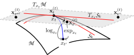
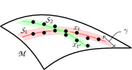
Consider a D𝐷D-dimensional Riemannian manifold \mathpzc{M} with metric g𝑔g. Based on g𝑔g, the (Riemannian) distance function distg(x,y)subscriptdist𝑔𝑥𝑦\operatorname{dist}_{g}(x,y) between points x,y𝑥𝑦x,y\in\mathpzc{M} is well-defined, and a geodesic is the (locally) distance-minimizing curve in \mathpzc{M} connecting x𝑥x and y𝑦y. Loosely speaking, geodesics generalize “straight lines” in Euclidean spaces to shortest paths in the “curved” \mathpzc{M} one. The RMMM hypothesis, which this paper advocates, postulates that the acquired data-points {xt}subscript𝑥𝑡\{x_{t}\} are located on or “close” to K𝐾K submanifolds (clusters) {𝒮𝓀}𝓀=1𝒦superscriptsubscriptsubscript𝒮𝓀𝓀1𝒦\{\mathpzc{S}_{k}\}_{k=1}^{K} of \mathpzc{M}, with possibly different dimensionalities. In contrast to the prevailing hypothesis for Kmeans, clusters in RMMM are allowed to have non-empty intersection. To accommodate noise and mis-modeling errors, data {xt}subscript𝑥𝑡\{x_{t}\} are considered to lie within the following γ𝛾\gamma-width (γ>0𝛾subscriptabsent0\gamma\in\mathbb{R}_{>0}) tubular neighborhood {x\nonscript|\nonscript(𝓈,𝓀)×{1,,𝒦}s.t.𝓈𝒮𝓀anddist(𝓍,𝓈)<γ}conditional-set𝑥\nonscript\nonscript𝓈𝓀1𝒦s.t.𝓈subscript𝒮𝓀andsubscriptdist𝓍𝓈𝛾\{x\in\mathpzc{M}\nonscript\,|\allowbreak\nonscript\,\mathopen{}\exists(s,k)\in\mathpzc{M}\times\{1,\ldots,K\}\ \text{s.t.}\ s\in\mathpzc{S}_{k}\ \text{and}\ \operatorname{dist}_{g}(x,s)<\gamma\}; see Fig. 3a. If Txtsubscript𝑇subscript𝑥𝑡T_{x_{t}}\mathpzc{M} denotes the tangent space of \mathpzc{M} at xtsubscript𝑥𝑡x_{t} (a D𝐷D-dimensional Euclidean space; see Fig. 3b), and assuming that xtsubscript𝑥𝑡x_{t} is located on a submanifold 𝒮𝓀subscript𝒮𝓀\mathpzc{S}_{k}, then Txt𝒮𝓀subscript𝑇subscript𝑥𝑡subscript𝒮𝓀T_{x_{t}}\mathpzc{S}_{k} stands for the tangent space of the dksubscript𝑑𝑘d_{k}-dimensional (dk<Dsubscript𝑑𝑘𝐷d_{k}<D) submanifold 𝒮𝓀subscript𝒮𝓀\mathpzc{S}_{k} at xtsubscript𝑥𝑡x_{t}. Loosely speaking, the exponential map expxt()subscriptsubscript𝑥𝑡\exp_{x_{t}}(\cdot) maps a D𝐷D-dimensional tangent vector 𝐯Txt𝐯subscript𝑇subscript𝑥𝑡\mathbf{v}\in T_{x_{t}}\mathpzc{M} to a point expxt(𝐯)subscriptsubscript𝑥𝑡𝐯\exp_{x_{t}}(\mathbf{v})\in\mathpzc{M}. If 𝒮𝓀subscript𝒮𝓀\mathpzc{S}_{k} is geodesic, i.e., it contains the geodesic defined by any two of its points, then 𝒮𝓀subscript𝒮𝓀\mathpzc{S}_{k} becomes the image of Txt𝒮𝓀subscript𝑇subscript𝑥𝑡subscript𝒮𝓀T_{x_{t}}\mathpzc{S}_{k} under expxtsubscriptsubscript𝑥𝑡\exp_{x_{t}}. The functional inverse of expxtsubscriptsubscript𝑥𝑡\exp_{x_{t}} is the logarithm map logxt:𝒯𝓍𝓉:subscriptsubscript𝑥𝑡subscript𝒯subscript𝓍𝓉\log_{x_{t}}:\mathpzc{M}\to T_{x_{t}}\mathpzc{M}, which maps xtsubscript𝑥𝑡x_{t} to the origin 𝟎0\mathbf{0} of Txtsubscript𝑇subscript𝑥𝑡T_{x_{t}}\mathpzc{M}. Let 𝐱t(t)superscriptsubscript𝐱superscript𝑡𝑡\mathbf{x}_{t^{\prime}}^{(t)} denote the image of a data point xtsubscript𝑥superscript𝑡x_{t^{\prime}} via the logarithm map at xtsubscript𝑥𝑡x_{t}, i.e., 𝐱t(t):=logxt(xt)assignsuperscriptsubscript𝐱superscript𝑡𝑡subscriptsubscript𝑥𝑡subscript𝑥superscript𝑡\mathbf{x}_{t^{\prime}}^{(t)}:=\log_{x_{t}}(x_{t^{\prime}}). Having the number of clusters/submanifolds K𝐾K known, the goal is to cluster data-set 𝒳:={𝓍𝓉}𝓉𝒯assign𝒳subscriptsubscript𝓍𝓉𝓉𝒯\mathpzc{X}:=\{x_{t}\}_{t\in\mathpzc{T}} (𝒯={1,,𝒯τw+1}𝒯1𝒯subscript𝜏w1\mathpzc{T}=\{1,\ldots,T-\tau_{\text{w}}+1\} in the context of Secs. II and III) into K𝐾K groups {𝒳𝓀}𝓀=1𝒦superscriptsubscriptsubscript𝒳𝓀𝓀1𝒦\{\mathpzc{X}_{k}\}_{k=1}^{K}\subset\mathpzc{M} s.t. points in 𝒳𝓀subscript𝒳𝓀\mathpzc{X}_{k} are associated with the submanifold 𝒮𝓀subscript𝒮𝓀\mathpzc{S}_{k}. Note that if \mathpzc{M} is a Euclidean space, and submanifolds are affine subspaces, then RMMM boils down to the subspace-clustering modeling [77].
Refer to caption
(a) Riemannian multi-manifold modeling (RMMM)
Refer to caption
(b) Logarithm and exponential map
Refer to caption
(c) Estimating tangent spaces
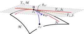
Figure 3: Two (K=2𝐾2K=2) submanifolds/clusters 𝒮1,𝒮2subscript𝒮1subscript𝒮2\mathpzc{S}_{1},\mathpzc{S}_{2} and their tubular neighborhoods on the Riemannian manifold \mathpzc{M}, as well as the associated exponential and logarithm maps. In contrast to classical Kmeans, clusters are allowed here to have non-empty intersection.

IV-B Algorithm

Since the submanifold 𝒮𝓀subscript𝒮𝓀\mathpzc{S}_{k}, that point xtsubscript𝑥𝑡x_{t} belongs to, is unknown, so is Txt𝒮𝓀subscript𝑇subscript𝑥𝑡subscript𝒮𝓀T_{x_{t}}\mathpzc{S}_{k}. To this end, an estimate of Txt𝒮𝓀subscript𝑇subscript𝑥𝑡subscript𝒮𝓀T_{x_{t}}\mathpzc{S}_{k}, denoted by T^xt𝒮subscript^𝑇subscript𝑥𝑡𝒮\hat{T}_{x_{t}}\mathpzc{S}, is associated with each point xtsubscript𝑥𝑡x_{t} of the data-set. Given a user-defined parameter NNNGCT>0superscriptsubscript𝑁NNGCTsubscriptabsent0N_{\text{NN}}^{\text{GCT}}\in\mathbb{Z}_{>0}, let the neighborhood

𝒯NN,𝓉GCT:={𝓉𝒯\nonscript|\nonscript𝓍𝓉is one of the𝒩NNGCTnearest neighbors of𝓍𝓉},assignsuperscriptsubscript𝒯NN𝓉GCTconditional-setsuperscript𝓉𝒯\nonscript\nonscriptmissing-subexpressionsubscript𝓍superscript𝓉is one of thesuperscriptsubscript𝒩NNGCTmissing-subexpressionnearest neighbors ofsubscript𝓍𝓉\displaystyle\mathpzc{T}_{\text{NN},t}^{\text{GCT}}:=\left\{t^{\prime}\in\mathpzc{T}\nonscript\,\middle|\allowbreak\nonscript\,\mathopen{}\begin{aligned} &x_{t^{\prime}}\ \text{is one of the}\ N_{\text{NN}}^{\text{GCT}}\\ &\text{nearest neighbors of}\ x_{t}\end{aligned}\right\}\,, (16)

where closeness is measured via distg(,)subscriptdist𝑔\operatorname{dist}_{g}(\cdot,\cdot), and define 𝐂^xtsubscript^𝐂subscript𝑥𝑡\hat{\mathbf{C}}_{x_{t}} as the “local” sample correlation matrix

𝐂^xt:=1NNNGCT1t𝒯NN,𝓉GCT𝐱t(t)𝐱t(t).\displaystyle\hat{\mathbf{C}}_{x_{t}}:=\tfrac{1}{N_{\text{NN}}^{\text{GCT}}-1}\sum\nolimits_{t^{\prime}\in\mathpzc{T}_{\text{NN},t}^{\text{GCT}}}\mathbf{x}_{t^{\prime}}^{(t)}\mathbf{x}_{t^{\prime}}^{(t)}{}^{\top}\,. (17)

Moreover, let 𝐂^xt=λmax(𝐂^xt)delimited-∥∥subscript^𝐂subscript𝑥𝑡subscript𝜆subscript^𝐂subscript𝑥𝑡\lVert\hat{\mathbf{C}}_{x_{t}}\rVert=\lambda_{\max}(\hat{\mathbf{C}}_{x_{t}}) denote the spectral norm of 𝐂^xtsubscript^𝐂subscript𝑥𝑡\hat{\mathbf{C}}_{x_{t}} as the maximum eigenvalue of the PSD 𝐂^xtsubscript^𝐂subscript𝑥𝑡\hat{\mathbf{C}}_{x_{t}}. Assuming that xtsubscript𝑥𝑡x_{t} lies close (in the Riemannian-distance sense) to submanifold 𝒮𝓀subscript𝒮𝓀\mathpzc{S}_{k}, estimates of the dimension dksubscript𝑑𝑘d_{k} of 𝒮𝓀subscript𝒮𝓀\mathpzc{S}_{k}, or equivalently, of Txt𝒮𝓀subscript𝑇subscript𝑥𝑡subscript𝒮𝓀T_{x_{t}}\mathpzc{S}_{k}, can be obtained by identifying a principal eigenspace T^xt𝒮subscript^𝑇subscript𝑥𝑡𝒮\hat{T}_{x_{t}}\mathpzc{S} of 𝐂^xtsubscript^𝐂subscript𝑥𝑡\hat{\mathbf{C}}_{x_{t}} via PCA arguments. Any method of estimating a principal eigenspace can be employed here; e.g., define T^xt𝒮subscript^𝑇subscript𝑥𝑡𝒮\hat{T}_{x_{t}}\mathpzc{S} as the linear subspace spanned by the eigenvalues larger than or equal to ηλmax(𝐂^xt)𝜂subscript𝜆subscript^𝐂subscript𝑥𝑡\eta\lambda_{\max}(\hat{\mathbf{C}}_{x_{t}}), for a user-defined parameter η(0,1)𝜂01\eta\in(0,1) (cf[6]). An illustration of T^xt𝒮subscript^𝑇subscript𝑥𝑡𝒮\hat{T}_{x_{t}}\mathpzc{S} can be found in Fig. 3c. If l(xt,xt)𝑙subscript𝑥𝑡subscript𝑥superscript𝑡l(x_{t},x_{t^{\prime}}) denotes the (shortest) geodesic connecting xtsubscript𝑥𝑡x_{t} and xtsubscript𝑥superscript𝑡x_{t^{\prime}} in \mathpzc{M}, and upon defining the tangent vector 𝐯tt:=logxt(xt)assignsubscript𝐯𝑡superscript𝑡subscriptsubscript𝑥𝑡subscript𝑥superscript𝑡\mathbf{v}_{tt^{\prime}}:=\log_{x_{t}}(x_{t^{\prime}}), standing as the “velocity” of l(xt,xt)𝑙subscript𝑥𝑡subscript𝑥superscript𝑡l(x_{t},x_{t^{\prime}}) at xtsubscript𝑥𝑡x_{t}, let the (empirical geodesic) angle θttsubscript𝜃𝑡superscript𝑡\theta_{tt^{\prime}} be defined as the angle between 𝐯ttsubscript𝐯𝑡superscript𝑡\mathbf{v}_{tt^{\prime}} and the estimated linear subspace T^xt𝒮subscript^𝑇subscript𝑥𝑡𝒮\hat{T}_{x_{t}}\mathpzc{S} of Txtsubscript𝑇subscript𝑥𝑡T_{x_{t}}\mathpzc{M}.

1:Manifold \mathpzc{M}; number of clusters K𝐾K; dataset {xt}t𝒯subscriptsubscript𝑥𝑡𝑡𝒯\{x_{t}\}_{t\in\mathpzc{T}}; the number of nearest neighbors NNNGCTsuperscriptsubscript𝑁NNGCTN_{\text{NN}}^{\text{GCT}}; distance parameter σdsubscript𝜎𝑑\sigma_{d} (default σd=1subscript𝜎𝑑1\sigma_{d}=1); angle parameter σasubscript𝜎𝑎\sigma_{a} (default σa=1subscript𝜎𝑎1\sigma_{a}=1); eigenvalue threshold η(0,1)𝜂01\eta\in(0,1).
2:Data-cluster associations.
3:for t=1,,|𝒯|𝑡1𝒯t=1,\ldots,\lvert\mathpzc{T}\rvert do
4:    Define neighborhood 𝒯NN,𝓉GCTsuperscriptsubscript𝒯NN𝓉GCT\mathpzc{T}_{\text{NN},t}^{\text{GCT}} [cf. (16)].
5:    Compute 𝐱t(t)=logxt(xt)superscriptsubscript𝐱superscript𝑡𝑡subscriptsubscript𝑥𝑡subscript𝑥superscript𝑡\mathbf{x}_{t^{\prime}}^{(t)}=\log_{x_{t}}(x_{t^{\prime}}), t𝒯NN,𝓉GCTfor-allsuperscript𝑡superscriptsubscript𝒯NN𝓉GCT\forall t^{\prime}\in\mathpzc{T}_{\text{NN},t}^{\text{GCT}}.
6:    (Local sparse coding:) Identify weights {αtt}t𝒯subscriptsubscript𝛼𝑡superscript𝑡superscript𝑡𝒯\{\alpha_{tt^{\prime}}\}_{t^{\prime}\in\mathpzc{T}} via (19).
7:    Compute the sample correlation matrix 𝐂^xtsubscript^𝐂subscript𝑥𝑡\hat{\mathbf{C}}_{x_{t}} by (17).
8:    (Local PCA:) Identify the eigenvalues which are larger than or equal to ηλmax(𝐂^xt)𝜂subscript𝜆subscript^𝐂subscript𝑥𝑡\eta\lambda_{\max}(\hat{\mathbf{C}}_{x_{t}}), and call the eigenspace spanned by the associated eigenvalues T^xt𝒮subscript^𝑇subscript𝑥𝑡𝒮\hat{T}_{x_{t}}\mathcal{S}.
9:    (Angular information:) Compute the empirical geodesic angles {θtt}t𝒯subscriptsubscript𝜃𝑡superscript𝑡superscript𝑡𝒯\{\theta_{tt^{\prime}}\}_{t^{\prime}\in\mathpzc{T}}.
10:end for
11:Form the |𝒯|×|𝒯|𝒯𝒯\lvert\mathpzc{T}\rvert\times\lvert\mathpzc{T}\rvert affinity matrix 𝐖:=[wtt](t,t)𝒯2assign𝐖subscriptdelimited-[]subscript𝑤𝑡superscript𝑡𝑡superscript𝑡superscript𝒯2\mathbf{W}:=[w_{tt^{\prime}}]_{(t,t^{\prime})\in\mathpzc{T}^{2}} as
wtt:=exp(|αtt|+|αtt|)exp(θtt+θttσa).assignsubscript𝑤𝑡superscript𝑡subscript𝛼𝑡superscript𝑡subscript𝛼superscript𝑡𝑡subscript𝜃𝑡superscript𝑡subscript𝜃superscript𝑡𝑡subscript𝜎𝑎\displaystyle w_{tt^{\prime}}:=\exp(|\alpha_{tt^{\prime}}|+|\alpha_{t^{\prime}t}|)\cdot\exp\left(-\tfrac{\theta_{tt^{\prime}}+\theta_{t^{\prime}t}}{\sigma_{a}}\right)\,. (18)
12:Apply spectral clustering [78] to 𝐖𝐖\mathbf{W} to identify data-cluster associations.
Algorithm 3 Geodesic clustering by tangent spaces (GCT).

Motivated by a very recent line of research [79, 80], this paper advocates the geodesic clustering by tangent spaces (GCT) algorithm, detailed in Alg. 3, to solve the clustering task at hand. Key-points of GCT are the local sparse coding of step 6, local PCA of step 8, and the extraction of the angular information at step 9. Regarding the sparse-coding step, after mapping data-points {xt}t𝒯subscriptsubscript𝑥𝑡𝑡𝒯\{x_{t}\}_{t\in\mathpzc{T}} to vectors {𝐱t(t)}t𝒯subscriptsuperscriptsubscript𝐱superscript𝑡𝑡superscript𝑡𝒯\{\mathbf{x}_{t^{\prime}}^{(t)}\}_{t^{\prime}\in\mathpzc{T}} in the tangent space Txtsubscript𝑇subscript𝑥𝑡T_{x_{t}}\mathpzc{M} at xtsubscript𝑥𝑡x_{t}, and motivated by the affine geometry of Txtsubscript𝑇subscript𝑥𝑡T_{x_{t}}\mathpzc{M} (cf. Fig. 3b), “relations” between data within neighborhood 𝒯NN,𝓉GCTsuperscriptsubscript𝒯NN𝓉GCT\mathpzc{T}_{\text{NN},t}^{\text{GCT}}, centered at 𝐱t(t)superscriptsubscript𝐱𝑡𝑡\mathbf{x}_{t}^{(t)}, are captured by the amount that neighbors {𝐱t(t)}t𝒯NN,𝓉GCT{𝓉}subscriptsuperscriptsubscript𝐱superscript𝑡𝑡superscript𝑡superscriptsubscript𝒯NN𝓉GCT𝓉\{\mathbf{x}_{t^{\prime}}^{(t)}\}_{t^{\prime}\in\mathpzc{T}_{\text{NN},t}^{\text{GCT}}\setminus\{t\}} (𝐱t(t)superscriptsubscript𝐱superscript𝑡𝑡\mathbf{x}_{t^{\prime}}^{(t)}, 𝐱t′′(t)superscriptsubscript𝐱superscript𝑡′′𝑡\mathbf{x}_{t^{\prime\prime}}^{(t)} and 𝐱t′′′(t)superscriptsubscript𝐱superscript𝑡′′′𝑡\mathbf{x}_{t^{\prime\prime\prime}}^{(t)} in Fig. 3b, for example) contribute in the description of 𝐱t(t)superscriptsubscript𝐱𝑡𝑡\mathbf{x}_{t}^{(t)} via affine combinations:

min{αtt}t𝒯NN,𝓉GCT{𝓉}subscriptsubscriptsubscript𝛼𝑡superscript𝑡superscript𝑡superscriptsubscript𝒯NN𝓉GCT𝓉\displaystyle\min_{\{\alpha_{tt^{\prime}}\}_{t^{\prime}\in\mathpzc{T}_{\text{NN},t}^{\text{GCT}}\setminus\{t\}}}\ 𝐱t(t)t𝒯NN,𝓉GCT{𝓉}αtt𝐱t(t)22Data-fit termsuperscriptsuperscriptsubscriptdelimited-∥∥superscriptsubscript𝐱𝑡𝑡subscriptsuperscript𝑡superscriptsubscript𝒯NN𝓉GCT𝓉subscript𝛼𝑡superscript𝑡superscriptsubscript𝐱superscript𝑡𝑡22Data-fit term\displaystyle\overbrace{\left\lVert\mathbf{x}_{t}^{(t)}-\sum\nolimits_{t^{\prime}\in\mathpzc{T}_{\text{NN},t}^{\text{GCT}}\setminus\{t\}}\alpha_{tt^{\prime}}\mathbf{x}_{t^{\prime}}^{(t)}\right\rVert_{2}^{2}}^{\text{Data-fit term}}
+t𝒯NN,𝓉GCT{𝓉}exp(𝐱t(t)𝐱t(t)2σd)|αtt|Sparsity-promoting termsubscriptsubscriptsuperscript𝑡superscriptsubscript𝒯NN𝓉GCT𝓉subscriptdelimited-∥∥superscriptsubscript𝐱𝑡𝑡superscriptsubscript𝐱superscript𝑡𝑡2subscript𝜎𝑑subscript𝛼𝑡superscript𝑡Sparsity-promoting term\displaystyle+\underbrace{\sum_{t^{\prime}\in\mathpzc{T}_{\text{NN},t}^{\text{GCT}}\setminus\{t\}}\exp\left(\tfrac{\lVert\mathbf{x}_{t}^{(t)}-\mathbf{x}_{t^{\prime}}^{(t)}\rVert_{2}}{\sigma_{d}}\right)\lvert\alpha_{tt^{\prime}}\rvert}_{\text{Sparsity-promoting term}}
s.tot𝒯NN,𝓉GCT{𝓉}αtt=1,s.tosubscriptsuperscript𝑡superscriptsubscript𝒯NN𝓉GCT𝓉subscript𝛼𝑡superscript𝑡1\displaystyle\text{s.to}\ \sum\nolimits_{t^{\prime}\in\mathpzc{T}_{\text{NN},t}^{\text{GCT}}\setminus\{t\}}\alpha_{tt^{\prime}}=1\,, (19)

where the constraint in (19) manifests that neighbors should cooperate affinely to describe 𝐱t(t)superscriptsubscript𝐱𝑡𝑡\mathbf{x}_{t}^{(t)} in the data-fit term. The regularization term in (19) enforces sparsity in the previous representation by penalizing, thus eliminating, contributions from neighbors which are located far from 𝐱t(t)superscriptsubscript𝐱𝑡𝑡\mathbf{x}_{t}^{(t)} via the weights exp(𝐱t(t)𝐱t(t)2/σd)subscriptdelimited-∥∥superscriptsubscript𝐱𝑡𝑡superscriptsubscript𝐱superscript𝑡𝑡2subscript𝜎𝑑\exp(\lVert\mathbf{x}_{t}^{(t)}-\mathbf{x}_{t^{\prime}}^{(t)}\rVert_{2}/\sigma_{d}): the larger the distance of 𝐱t(t)superscriptsubscript𝐱superscript𝑡𝑡\mathbf{x}_{t^{\prime}}^{(t)} from 𝐱t(t)superscriptsubscript𝐱𝑡𝑡\mathbf{x}_{t}^{(t)} in the tangent space Txtsubscript𝑇subscript𝑥𝑡T_{x_{t}}\mathpzc{M}, the larger the penalty on the modulus of the affine coefficient αttsubscript𝛼𝑡superscript𝑡\alpha_{tt^{\prime}}. Moreover, no relations are established between 𝐱t(t)superscriptsubscript𝐱𝑡𝑡\mathbf{x}_{t}^{(t)} and data points {𝐱t(t)}t𝒯𝒯NN,𝓉GCTsubscriptsuperscriptsubscript𝐱superscript𝑡𝑡superscript𝑡𝒯superscriptsubscript𝒯NN𝓉GCT\{\mathbf{x}_{t^{\prime}}^{(t)}\}_{t^{\prime}\in\mathpzc{T}\setminus\mathpzc{T}_{\text{NN},t}^{\text{GCT}}} which do not belong to neighborhood 𝒯NN,𝓉GCTsuperscriptsubscript𝒯NN𝓉GCT\mathpzc{T}_{\text{NN},t}^{\text{GCT}}, by setting αtt:=0assignsubscript𝛼𝑡superscript𝑡0\alpha_{tt^{\prime}}:=0 for any t𝒯𝒯NN,𝓉GCTsuperscript𝑡𝒯superscriptsubscript𝒯NN𝓉GCTt^{\prime}\in\mathpzc{T}\setminus\mathpzc{T}_{\text{NN},t}^{\text{GCT}}. All information collected in weights {αtt}subscript𝛼𝑡superscript𝑡\{\alpha_{tt^{\prime}}\} and {θtt}subscript𝜃𝑡superscript𝑡\{\theta_{tt^{\prime}}\} are gathered in the affinity matrix 𝐖𝐖\mathbf{W} (step 12 of Alg. 3) that is fed in any spectral clustering (SC) algorithm that provides data-cluster associations. The contribution of GCT [79, 80] in clustering on Riemannian surfaces is the novel way of extraction and incorporation of the angular information {θtt}subscript𝜃𝑡superscript𝑡\{\theta_{tt^{\prime}}\} in an SC affinity matrix. A performance analysis, with guarantees on the clustering accuracy and the number of mis-classified data-points, has been already provided for a simplified version of GCT, where submanifolds are considered to be “geodesic,” justifying thus the name GCT, the sparse-coding scheme of step 6 in Alg. 3 is not employed, and the affinity matrix of step 12 becomes a binary one, with entries either 111 or 00, depending on whether conditions on the dimensions of the estimated tangent subspaces, the angular information {θtt}subscript𝜃𝑡superscript𝑡\{\theta_{tt^{\prime}}\} and the Riemannian distance between data-points are satisfied or not [79].

IV-C Computational complexity

A major part of GCT computations take place within the neighborhood 𝒯NN,𝓉GCTsuperscriptsubscript𝒯NN𝓉GCT\mathpzc{T}_{\text{NN},t}^{\text{GCT}}. The complexity for computing the NNNGCTsuperscriptsubscript𝑁NNGCTN_{\text{NN}}^{\text{GCT}} (typically 100absent100\leq 100 in all numerical tests) nearest neighbors of xtsubscript𝑥𝑡x_{t} is (|𝒯|𝒞dist+𝒩NNGCTlog|𝒯|)𝒯subscript𝒞distsuperscriptsubscript𝒩NNGCT𝒯(\lvert\mathpzc{T}\rvert\mathcal{C}_{\operatorname{dist}}+N_{\text{NN}}^{\text{GCT}}\log\lvert\mathpzc{T}\rvert), where 𝒞distsubscript𝒞dist\mathcal{C}_{\operatorname{dist}} denotes the cost of computing the Riemannian distance between any two points, |𝒯|𝒞dist𝒯subscript𝒞dist\lvert\mathpzc{T}\rvert\mathcal{C}_{\operatorname{dist}} refers to the complexity of computing |𝒯|1𝒯1\lvert\mathpzc{T}\rvert-1 distances, and NNNGCTlog|𝒯|superscriptsubscript𝑁NNGCT𝒯N_{\text{NN}}^{\text{GCT}}\log\lvert\mathpzc{T}\rvert refers to the effort of identifying the NNNGCTsuperscriptsubscript𝑁NNGCTN_{\text{NN}}^{\text{GCT}} nearest neighbors of xtsubscript𝑥𝑡x_{t}. Notice that once the logarithm map logxt(xt)subscriptsubscript𝑥𝑡subscript𝑥superscript𝑡\log_{x_{t}}(x_{t^{\prime}}) is computed, under complexity 𝒞logsubscript𝒞\mathcal{C}_{\log} (cf. Appendix B), then 𝒞dist=𝒪(dim)subscript𝒞dist𝒪dimension\mathcal{C}_{\operatorname{dist}}=\mathcal{O}(\dim\mathpzc{M}). If \mathpzc{M} is the set PD(N𝒢)PDsubscript𝑁𝒢\text{PD}(N_{\mathpzc{G}}), then 𝒞log=𝒪[(N𝒢(N𝒢+1)/2)3 ]subscript𝒞𝒪delimited-[](N𝒢(N𝒢+1)/2)3 \mathcal{C}_{\log}=\mathcal{O}[\mathchoice{{\hbox{$\displaystyle\sqrt{(N_{\mathpzc{G}}(N_{\mathpzc{G}}+1)/2)^{3}\,}$}\lower 0.4pt\hbox{\vrule height=9.30444pt,depth=-7.44359pt}}}{{\hbox{$\textstyle\sqrt{(N_{\mathpzc{G}}(N_{\mathpzc{G}}+1)/2)^{3}\,}$}\lower 0.4pt\hbox{\vrule height=9.30444pt,depth=-7.44359pt}}}{{\hbox{$\scriptstyle\sqrt{(N_{\mathpzc{G}}(N_{\mathpzc{G}}+1)/2)^{3}\,}$}\lower 0.4pt\hbox{\vrule height=6.53888pt,depth=-5.23112pt}}}{{\hbox{$\scriptscriptstyle\sqrt{(N_{\mathpzc{G}}(N_{\mathpzc{G}}+1)/2)^{3}\,}$}\lower 0.4pt\hbox{\vrule height=5.03888pt,depth=-4.03113pt}}}], while 𝒞log=𝒪(p2ρ2mN𝒢)subscript𝒞𝒪superscript𝑝2superscript𝜌2𝑚subscript𝑁𝒢\mathcal{C}_{\log}=\mathcal{O}(p^{2}\rho^{2}mN_{\mathpzc{G}}) if \mathpzc{M} is the Grassmannian Gr(mN𝒢,pρ)Gr𝑚subscript𝑁𝒢𝑝𝜌\text{Gr}(mN_{\mathpzc{G}},p\rho).

Step 6 of Alg. 3 requires solving the sparsity-promoting optimization task of (19). Notice that due to 2subscriptdelimited-∥∥2\lVert\>\cdot\>\rVert_{2}, only inner products of Euclidean vectors are necessary to form the loss function in (19), which entails a complexity of order 𝒪(dim)𝒪dimension\mathcal{O}(\dim\mathpzc{M}). Given that only NNNGCTsuperscriptsubscript𝑁NNGCTN_{\text{NN}}^{\text{GCT}} vectors are involved, (19) is a small-scale convex-optimization task that can be determined efficiently (let 𝒞scsubscript𝒞sc\mathcal{C}_{\text{sc}} denote that complexity) by any off-the-shelf solver [9]. Step 8 of Alg. 3 involves the computation of the top eigenvectors of the sample covariance matrix 𝐂^xtsubscript^𝐂subscript𝑥𝑡\hat{\mathbf{C}}_{x_{t}}, under complexity of 𝒪[dim+(𝒩NNGCT)3]𝒪delimited-[]dimensionsuperscriptsuperscriptsubscript𝒩NNGCT3\mathcal{O}[\dim\mathpzc{M}+(N_{\text{NN}}^{\text{GCT}})^{3}]. Finally, to compute the empirical geodesic angles, 𝒪(|𝒯|𝒞log+|𝒯|dim)𝒪𝒯subscript𝒞𝒯dimension\mathcal{O}(\lvert\mathpzc{T}\rvert\mathcal{C}_{\log}+\lvert\mathpzc{T}\rvert\dim\mathpzc{M}) operations are necessary. Spectral clustering is invoked in step 12 of Alg. 3 on the |𝒯|×|𝒯|𝒯𝒯\lvert\mathpzc{T}\rvert\times\lvert\mathpzc{T}\rvert affinity matrix 𝐖𝐖\mathbf{W}. Its main computational burden is to identify K𝐾K eigenvectors (K𝐾K is the number of clusters) of 𝐖𝐖\mathbf{W}, which entails complexity of order 𝒪(K|𝒯|2)𝒪𝐾superscript𝒯2\mathcal{O}(K\lvert\mathpzc{T}\rvert^{2}). To summarize, the complexity of GCT is 𝒪[|𝒯|2(𝒞dist+𝒞log+dim+𝒦)+𝒩NNGCT|𝒯|log|𝒯|+|𝒯|𝒞sc+|𝒯|dim+|𝒯|(𝒩NNGCT)3]𝒪delimited-[]superscript𝒯2subscript𝒞distsubscript𝒞dimension𝒦superscriptsubscript𝒩NNGCT𝒯𝒯𝒯subscript𝒞sc𝒯dimension𝒯superscriptsuperscriptsubscript𝒩NNGCT3\mathcal{O}[\lvert\mathpzc{T}\rvert^{2}(\mathcal{C}_{\operatorname{dist}}+\mathcal{C}_{\log}+\dim\mathpzc{M}+K)+N_{\text{NN}}^{\text{GCT}}\lvert\mathpzc{T}\rvert\log\lvert\mathpzc{T}\rvert+\lvert\mathpzc{T}\rvert\mathcal{C}_{\text{sc}}+\lvert\mathpzc{T}\rvert\dim\mathpzc{M}+\lvert\mathpzc{T}\rvert(N_{\text{NN}}^{\text{GCT}})^{3}].

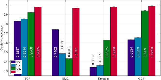
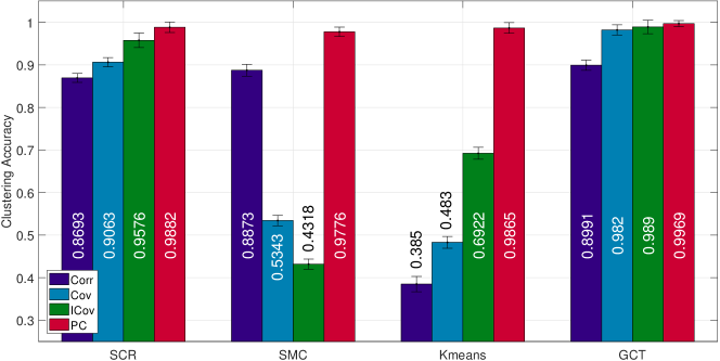
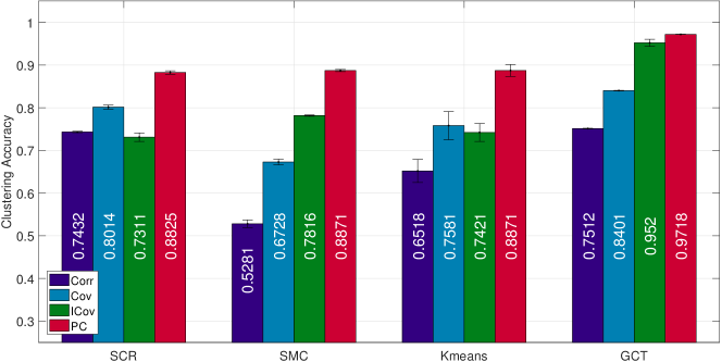
V Numerical tests

To assess performance, the proposed GCT algorithm is compared with the following methods:

  1. (i)

    Sparse manifold clustering (SMC) [24, 19]. SMC was introduced in [24] for clustering submanifolds within Euclidean spaces, and it was later modified in [19] for clustering submanifolds on the sphere. SMC is adapted here, according to our needs, to cluster submanifolds in a Riemannian manifold, and still referred to as SMC. SMC’s basic idea is as follows: Per each data-point x𝑥x, a local neighborhood is mapped to the tangent space Txsubscript𝑇𝑥T_{x}\mathpzc{M} by the logarithm map (cf. step 5 of Alg. 3), and a sparse-coding task (cf. step 6 of Alg. 3) is solved in Txsubscript𝑇𝑥T_{x}\mathpzc{M} to provide weights for an SC similarity matrix.

  2. (ii)

    Spectral clustering [78] equipped with Riemannian metric (SCR) of [27]. SCR [27] utilizes SC under the weighted affinity matrix [𝐖]tt:=exp[distg2(xt,xt)/(2σ2)]assignsubscriptdelimited-[]𝐖𝑡superscript𝑡superscriptsubscriptdist𝑔2subscript𝑥𝑡subscript𝑥superscript𝑡2superscript𝜎2[\mathbf{W}]_{tt^{\prime}}:=\exp[-\operatorname{dist}_{g}^{2}(x_{t},x_{t^{\prime}})/(2\sigma^{2})], where the Riemannian distance metric distg(,)subscriptdist𝑔\operatorname{dist}_{g}(\cdot,\cdot) is used to quantify affinity among data-points [27].

  3. (iii)

    Kmeans, where data lying in the Riemannian manifold are embedded into a Euclidean space, and then the classical Kmeans, under the classical (Euclidean) 2subscript2\ell_{2}-distance metric, is applied to the embedded dataset. In particular, Grassmannian manifolds are embedded into Euclidean spaces by the isometric embedding [45, 8], and PD(N𝒢)PDsubscript𝑁𝒢\text{PD}(N_{\mathpzc{G}}) is embedded into N𝒢(N𝒢+1)/2superscriptsubscript𝑁𝒢subscript𝑁𝒢12\mathbb{R}^{N_{\mathpzc{G}}(N_{\mathpzc{G}}+1)/2} by vectorizing the triangular upper part of the elements of PD(N𝒢)PDsubscript𝑁𝒢\text{PD}(N_{\mathpzc{G}}). This set of tests stands as a representative of all schemes that do not exploit the underlying Riemannian geometry, as detailed in Sec. I-B.

Unlike GCT, none of the previous methods utilizes the underlying submanifold tangential information (Kmeans is even Riemannian-geometry agnostic). In contrast to the prevailing hypothesis of Kmeans and variants, that clusters are not closely located to each other, RMMM allows for non-empty intersections of submanifolds (cf. Fig. 3a).

The ground-truth labels of clusters are available in each experiment, and assessment is done via the notion of clustering accuracy, defined as “(##\# of points with cluster labels equal to the ground-truth ones) // (##\# of total points).” Signal-to-noise ratio (SNR) is set to be 101010dB for all experiments. Tests are run for a number of 505050 realizations, and average clustering accuracies, as well as standard deviations, are depicted in the subsequent figures.

V-A Synthetically generated time series

This section refers to the setting of Fig. 1. Per state, there are up to three tasks/events/modules that need to be accomplished through the cooperation of nodes. Each node contributes to a specific task by sharing a common signal with other nodes assigned to the same task. Nodes that share a common task are considered to be connected to each other. Per node, the previous common signal is linearly combined with a signal characteristic of the node, and with a first-order auto-regressive (AR) process, with time-varying AR coefficient, contributing to the dynamics of the task-specific signal. The AR signal is described by the recursion yνt,AR:=cosθtyν(t1),AR+1cos2θt vtassignsubscript𝑦𝜈𝑡ARsubscript𝜃𝑡subscript𝑦𝜈𝑡1AR1cos2θt subscript𝑣𝑡y_{\nu t,\text{AR}}:=\cos\theta_{t}\cdot y_{\nu(t-1),\text{AR}}+\mathchoice{{\hbox{$\displaystyle\sqrt{1-\cos^{2}\theta_{t}\,}$}\lower 0.4pt\hbox{\vrule height=6.94444pt,depth=-5.55559pt}}}{{\hbox{$\textstyle\sqrt{1-\cos^{2}\theta_{t}\,}$}\lower 0.4pt\hbox{\vrule height=6.94444pt,depth=-5.55559pt}}}{{\hbox{$\scriptstyle\sqrt{1-\cos^{2}\theta_{t}\,}$}\lower 0.4pt\hbox{\vrule height=4.8611pt,depth=-3.8889pt}}}{{\hbox{$\scriptscriptstyle\sqrt{1-\cos^{2}\theta_{t}\,}$}\lower 0.4pt\hbox{\vrule height=3.47221pt,depth=-2.77779pt}}}\cdot v_{t}, where vtsubscript𝑣𝑡v_{t} is a zero-mean and unit-variance normal r.v., and θt:=θt1+Δθassignsubscript𝜃𝑡subscript𝜃𝑡1Δ𝜃\theta_{t}:=\theta_{t-1}+\Delta\theta, for some user-defined parameters θ0subscript𝜃0\theta_{0} and ΔθΔ𝜃\Delta\theta. The linear combination of all the previous time series is filtered by the model of [62] to yield the BOLD data {𝐲t}t=1Tsuperscriptsubscriptsubscript𝐲𝑡𝑡1𝑇\{\mathbf{y}_{t}\}_{t=1}^{T}.

Regarding Alg. 1 of Sec. II, parameters are set as follows: N𝒢:=10assignsubscript𝑁𝒢10N_{\mathpzc{G}}:=10, m=3𝑚3m=3, p=1𝑝1p=1, ρ=3𝜌3\rho=3, τf=20subscript𝜏f20\tau_{\text{f}}=20, τb=20subscript𝜏b20\tau_{\text{b}}=20, and τw{50,70,80}subscript𝜏w507080\tau_{\text{w}}\in\{50,70,80\}. Results pertaining to the observability-matrix features of Sec. II are denoted by the “OB” tag in the legents of all subsequent figures.

Regarding the methodology of Sec. III, several features are explored in the numerical tests. More specifically, with reference to (11), point xtPD(N𝒢)subscript𝑥𝑡PDsubscript𝑁𝒢x_{t}\in\text{PD}(N_{\mathpzc{G}}) takes the following values: (i) (diag𝐊t1)1/2𝐊t1(diag𝐊t1)1/2superscriptdiagsuperscriptsubscript𝐊𝑡112superscriptsubscript𝐊𝑡1superscriptdiagsuperscriptsubscript𝐊𝑡112(\operatorname{diag}\mathbf{K}_{t}^{-1})^{-1/2}\mathbf{K}_{t}^{-1}(\operatorname{diag}\mathbf{K}_{t}^{-1})^{-1/2}from step 10 of Alg. 2, denoted by the tag “kPC” in the subsequent figures; (ii) 𝐊tsubscript𝐊𝑡\mathbf{K}_{t}from step 8 of Alg. 2, denoted by tag “Cov”; (iii) 𝐊t1superscriptsubscript𝐊𝑡1\mathbf{K}_{t}^{-1}, denoted by tag “ICov”; and (iv) 𝚲tsubscript𝚲𝑡\bm{\Lambda}_{t}, where [𝚲t]νν:=κ(𝒚νt,𝒚νt)assignsubscriptdelimited-[]subscript𝚲𝑡𝜈superscript𝜈𝜅subscript𝒚𝜈𝑡subscript𝒚superscript𝜈𝑡[\bm{\Lambda}_{t}]_{\nu\nu^{\prime}}:=\kappa(\bm{y}_{\nu t},\bm{y}_{\nu^{\prime}t}), with {𝒚νt}ν=1N𝒢superscriptsubscriptsubscript𝒚𝜈𝑡𝜈1subscript𝑁𝒢\{\bm{y}_{\nu t}\}_{\nu=1}^{N_{\mathpzc{G}}} being the rows of 𝐘t:=[𝐲t,𝐲t+1,,𝐲t+τw1]assignsubscript𝐘𝑡subscript𝐲𝑡subscript𝐲𝑡1subscript𝐲𝑡subscript𝜏w1\mathbf{Y}_{t}:=[\mathbf{y}_{t},\mathbf{y}_{t+1},\ldots,\mathbf{y}_{t+\tau_{\text{w}}-1}], and denoted by tag “Corr”.

Constructing a reproducing kernel function κ𝜅\kappa, or the sequence of kernel matrices {𝐊t}subscript𝐊𝑡\{\mathbf{K}_{t}\} in step 6 of Alg. 2, plays a principal role in the methodology of Sec. III. To this end and along the lines of Sec. III-A, four ways of designing the kernel matrices are explored:

  1. (i)

    Linear kernel function: By choosing κlsubscript𝜅l\kappa_{\text{l}} of Appendix A as the kernel function, the feature space \mathpzc{H} becomes nothing but the input Euclidean τwsuperscriptsubscript𝜏w\mathbb{R}^{\tau_{\text{w}}} one, with κl(𝒚,𝒚)=𝒚𝒚\kappa_{\text{l}}(\bm{y},\bm{y}^{\prime})=\bm{y}\bm{y}^{\prime}{}^{\top}, for any 𝒚,𝒚τw𝒚superscript𝒚superscriptsubscript𝜏w\bm{y},\bm{y}^{\prime}\in\mathbb{R}^{\tau_{\text{w}}}. As such, the previously met 𝐊tsubscript𝐊𝑡\mathbf{K}_{t} and 𝚲tsubscript𝚲𝑡\bm{\Lambda}_{t} become the classical covariance and correlation matrices, respectively. As Figs. 48 demonstrate, the larger the values of the sliding window τwsubscript𝜏w\tau_{\text{w}} and the number of nearest neighbors NNNGCDsuperscriptsubscript𝑁NNGCDN_{\text{NN}}^{\text{GCD}} are, the better all methods perform. However, GCT exhibits the best performance even for small values of those parameters, particularly for the advocated features of kPC and observability matrices (“OB”). Further, focusing on these two features, it can be seen that “OB” outperforms kPC in almost all scenarios.
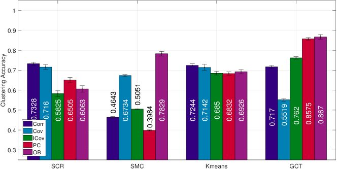
    Refer to caption
    Figure 4: Linear kernel: τw=50subscript𝜏w50\tau_{\text{w}}=50; NNNGCD=12superscriptsubscript𝑁NNGCD12N_{\text{NN}}^{\text{GCD}}=12.
    Refer to caption
    Figure 5: Linear kernel: τw=70subscript𝜏w70\tau_{\text{w}}=70; NNNGCT=12superscriptsubscript𝑁NNGCT12N_{\text{NN}}^{\text{GCT}}=12.
    Refer to caption
    Figure 6: Linear kernel: τw=80subscript𝜏w80\tau_{\text{w}}=80; NNNGCT=8superscriptsubscript𝑁NNGCT8N_{\text{NN}}^{\text{GCT}}=8.
    Refer to caption
    Figure 7: Linear kernel: τw=80subscript𝜏w80\tau_{\text{w}}=80; NNNGCT=12superscriptsubscript𝑁NNGCT12N_{\text{NN}}^{\text{GCT}}=12.
    Refer to caption
    Figure 8: Linear kernel: τw=80subscript𝜏w80\tau_{\text{w}}=80; NNNGCT=16superscriptsubscript𝑁NNGCT16N_{\text{NN}}^{\text{GCT}}=16.
  2. (ii)

    Single Gaussian kernel function: The Gaussian (reproducing) kernel function κσsubscript𝜅𝜎\kappa_{\sigma} of Appendix A is used here, with variance values σ2{0.5,1,2}superscript𝜎20.512\sigma^{2}\in\{0.5,1,2\}. As Appendix A suggests, the feature space σsubscript𝜎\mathpzc{H}_{\sigma} becomes an infinite-dimensional functional space. Notice that the “OB” tag is not included in Figs. 914, since the methodology of Sec. II does not include any kernel-based arguments. As the relevant figures demonstrate, all methods appear to be sensitive to the choice of the kernel’s variance value: the less the value is, the worse the clustering accuracies become. Still, under such a uniform behavior, GCT exhibits the best performance among employed methods.
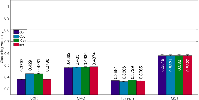
    Refer to caption
    Figure 9: Single Gaussian kernel: σ2=0.5superscript𝜎20.5\sigma^{2}=0.5; τw=50subscript𝜏w50\tau_{\text{w}}=50; NNNGCT=16superscriptsubscript𝑁NNGCT16N_{\text{NN}}^{\text{GCT}}=16.
    Refer to caption
    Figure 10: Single Gaussian kernel: σ2=1superscript𝜎21\sigma^{2}=1; τw=50subscript𝜏w50\tau_{\text{w}}=50; NNNGCT=16superscriptsubscript𝑁NNGCT16N_{\text{NN}}^{\text{GCT}}=16.
    Refer to caption
    Figure 11: Single Gaussian kernel: σ2=2superscript𝜎22\sigma^{2}=2; τw=50subscript𝜏w50\tau_{\text{w}}=50; NNNGCT=16superscriptsubscript𝑁NNGCT16N_{\text{NN}}^{\text{GCT}}=16.
    Refer to caption
    Figure 12: Single Gaussian kernel: σ2=0.5superscript𝜎20.5\sigma^{2}=0.5; τw=80subscript𝜏w80\tau_{\text{w}}=80; NNNGCT=16superscriptsubscript𝑁NNGCT16N_{\text{NN}}^{\text{GCT}}=16.
    Refer to caption
    Figure 13: Single Gaussian kernel: σ2=1superscript𝜎21\sigma^{2}=1; τw=80subscript𝜏w80\tau_{\text{w}}=80; NNNGCT=16superscriptsubscript𝑁NNGCT16N_{\text{NN}}^{\text{GCT}}=16.
    Refer to caption
    Figure 14: Single Gaussian kernel: σ2=2superscript𝜎22\sigma^{2}=2; τw=80subscript𝜏w80\tau_{\text{w}}=80; NNNGCT=16superscriptsubscript𝑁NNGCT16N_{\text{NN}}^{\text{GCT}}=16.
  3. (iii)

    Multi-kernel function: As Figs. 914 demonstrate, the choice of the value of variance of a Gaussian kernel hinders the clustering-accuracy performance of all employed techniques. To this end, a multi-kernel-function approach is adopted here to robustify all methods: κ:=(1/I)i=1Iκσiassign𝜅1𝐼superscriptsubscript𝑖1𝐼subscript𝜅subscript𝜎𝑖\kappa:=(1/I)\sum_{i=1}^{I}\kappa_{\sigma_{i}}, where the values of variances cover the wide range σi{0.25+0.01(i1)}i=1Isubscript𝜎𝑖superscriptsubscript0.250.01𝑖1𝑖1𝐼\sigma_{i}\in\{0.25+0.01(i-1)\}_{i=1}^{I}, with I:=376assign𝐼376I:=376, σ1=0.25subscript𝜎10.25\sigma_{1}=0.25, and σI=4subscript𝜎𝐼4\sigma_{I}=4. It can be easily verified that κ𝜅\kappa is a reproducing kernel (cf. Appendix A). Moreover, the resulting feature space \mathpzc{H} is an infinite-dimensional functional space. Needless to say that there are numerous ways of defining similar multi-kernel functions, such as the incorporation of polynomial or linear kernels in κ𝜅\kappa. Since this study is not meant to be exhaustive, such a path is not pursued. Figs. 1519 show results for several values of sliding-window length τwsubscript𝜏w\tau_{\text{w}} and NNNGCTsuperscriptsubscript𝑁NNGCTN_{\text{NN}}^{\text{GCT}}. As expected, multi-kernel functions enhance performance of all methods, with GCT exhibiting the best performance among employed techniques.
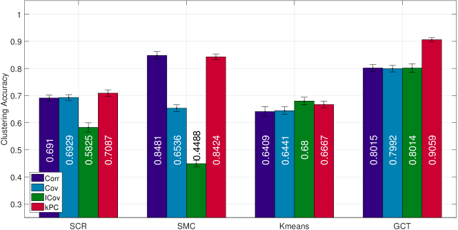
    Refer to caption
    Figure 15: Multi-kernel: τw=50subscript𝜏w50\tau_{\text{w}}=50; NNNGCT=12superscriptsubscript𝑁NNGCT12N_{\text{NN}}^{\text{GCT}}=12.
    Refer to caption
    Figure 16: Multi-kernel: τw=70subscript𝜏w70\tau_{\text{w}}=70; NNNGCT=12superscriptsubscript𝑁NNGCT12N_{\text{NN}}^{\text{GCT}}=12.
    Refer to caption
    Figure 17: Multi-kernel: τw=80subscript𝜏w80\tau_{\text{w}}=80; NNNGCT=8superscriptsubscript𝑁NNGCT8N_{\text{NN}}^{\text{GCT}}=8.
    Refer to caption
    Figure 18: Multi-kernel: τw=80subscript𝜏w80\tau_{\text{w}}=80; NNNGCT=12superscriptsubscript𝑁NNGCT12N_{\text{NN}}^{\text{GCT}}=12.
    Refer to caption
    Figure 19: Multi-kernel: τw=80subscript𝜏w80\tau_{\text{w}}=80; NNNGCT=16superscriptsubscript𝑁NNGCT16N_{\text{NN}}^{\text{GCT}}=16.
  4. (iv)

    SDE: Here, the kernel function is designed via the data-driven approach of Sec. III-A3, and results are demonstrated in Figs. 2022. To be able to vary meaningfully the neighborhood sizes {NνtSDE}subscriptsuperscript𝑁SDE𝜈𝑡\{N^{\text{SDE}}_{\nu t}\}, needed as parameters in SDE, the brain-network size N𝒢subscript𝑁𝒢N_{\mathpzc{G}} took the values of 101010 and 505050. As Figs. 2022 exhibit, the larger the network and SDE-neighborhood size are, the better SDE performs.
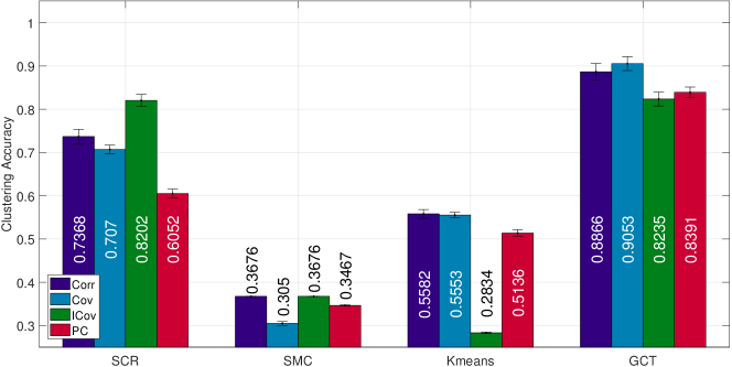
    Refer to caption
    Figure 20: SDE: NνtSDE=3subscriptsuperscript𝑁SDE𝜈𝑡3N^{\text{SDE}}_{\nu t}=3; N𝒢=10subscript𝑁𝒢10N_{\mathpzc{G}}=10; NNNGCT=16superscriptsubscript𝑁NNGCT16N_{\text{NN}}^{\text{GCT}}=16.
    Refer to caption
    Figure 21: SDE: NνtSDE=10subscriptsuperscript𝑁SDE𝜈𝑡10N^{\text{SDE}}_{\nu t}=10; N𝒢=50subscript𝑁𝒢50N_{\mathpzc{G}}=50; NNNGCT=16superscriptsubscript𝑁NNGCT16N_{\text{NN}}^{\text{GCT}}=16.
    Refer to caption
    Figure 22: SDE: NνtSDE=20subscriptsuperscript𝑁SDE𝜈𝑡20N^{\text{SDE}}_{\nu t}=20; N𝒢=50subscript𝑁𝒢50N_{\mathpzc{G}}=50; NNNGCT=16superscriptsubscript𝑁NNGCT16N_{\text{NN}}^{\text{GCT}}=16.

The best clustering-accuracy result among Figs. 422 is recorded for GCT in Figs. 8 and 19, with a value of 111 for the “kPC” feature.

V-B Real-data-driven time series

The brain activity analyzed in this section was obtained by the spatially embedded nonlinear model of [49], and the structural brain networks derived from diffusion spectrum imaging (DSI) of the data collected from 444 healthy adult subjects. All subjects volunteered with informed consent in writing and in accordance with the Institutional Review Board/Human Subjects Committee, Univ. of California, Santa Barbara.
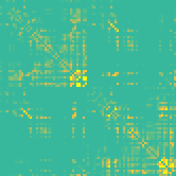
Refer to caption
(a) Subject 1
Refer to caption
(b) Subject 2
Refer to caption
(c) Subject 3
Refer to caption
(d) Subject 4
Figure 23: Real-data structural weighted adjacency matrices.

As described fully in [49], diffusion tractography was used to estimate the number of streamlines linking a number N𝒢=83subscript𝑁𝒢83N_{\mathpzc{G}}=83 of large-scale cortical and subcortical regions extracted from the Lausanne atlas [35]. The number of streamlines connecting two regions was normalized by the sum of the volumes of the regions, resulting in the weighted adjacency matrix 𝐁=[bνν]𝐁delimited-[]subscript𝑏𝜈superscript𝜈\mathbf{B}=[b_{\nu\nu^{\prime}}], where bννsubscript𝑏𝜈superscript𝜈b_{\nu\nu^{\prime}} reflects the density of streamlines connecting the ν𝜈\nuth and νsuperscript𝜈\nu^{\prime}th brain regions (Fig. 23). Additionally, the spatial distance between two brain regions was used to estimate the signal transmission time, assuming a signal propagation speed of 8m/sec8msec8\text{m}/\text{sec}.

Regional brain activity (EEG-type time series) was modeled using biologically motivated nonlinear Wilson-Cowan oscillators [83, 84]. Wilson-Cowan oscillators represent the mean-field dynamics of a spatially localized population of neurons, modeled through equations governing the firing rate of excitatory, yνtsubscript𝑦𝜈𝑡y_{\nu t}, and inhibitory, xνtsubscript𝑥𝜈𝑡x_{\nu t}, neuronal populations. As in [49], single Wilson-Cowan oscillators are linked as follows, via the individual’s adjacency and delay matrices which are unique for each of the four subjects:

dyνtdt𝑑subscript𝑦𝜈𝑡𝑑𝑡\displaystyle\tfrac{dy_{\nu t}}{dt} =\displaystyle= αyνt+ηyt𝛼subscript𝑦𝜈𝑡subscript𝜂𝑦𝑡\displaystyle-\alpha y_{\nu t}+\eta_{yt}
+0.9945yνt8fy(γ1yνtγ2xνt\displaystyle+\tfrac{0.9945-y_{\nu t}}{8}f_{y}\Bigl{(}\gamma_{1}y_{\nu t}-\gamma_{2}x_{\nu t}
+γ5ν=1N𝒢bννyν(tdνν)subscript𝛾5superscriptsubscriptsuperscript𝜈1subscript𝑁𝒢subscript𝑏𝜈superscript𝜈subscript𝑦superscript𝜈𝑡subscript𝑑𝜈superscript𝜈\displaystyle\hphantom{\frac{0.9945-y_{\nu t}}{8}f_{y}}+\gamma_{5}\sum\nolimits_{\nu^{\prime}=1}^{N_{\mathpzc{G}}}b_{\nu\nu^{\prime}}y_{\nu^{\prime}}(t-d_{\nu\nu^{\prime}})
+μνt),\displaystyle\hphantom{\frac{0.9945-y_{\nu t}}{8}f_{y}}+\mu_{\nu t}\Bigr{)}\,, (20a)
dxνtdt𝑑subscript𝑥𝜈𝑡𝑑𝑡\displaystyle\tfrac{dx_{\nu t}}{dt} =\displaystyle= αxνt+ηxt𝛼subscript𝑥𝜈𝑡subscript𝜂𝑥𝑡\displaystyle-\alpha x_{\nu t}+\eta_{xt}
+0.9994xνt8fx(γ3yνtγ4xνt),0.9994subscript𝑥𝜈𝑡8subscript𝑓𝑥subscript𝛾3subscript𝑦𝜈𝑡subscript𝛾4subscript𝑥𝜈𝑡\displaystyle+\tfrac{0.9994-x_{\nu t}}{8}f_{x}\bigl{(}\gamma_{3}y_{\nu t}-\gamma_{4}x_{\nu t}\bigr{)}\,, (20b)
fz(q)subscript𝑓𝑧𝑞\displaystyle f_{z}(q) :=assign\displaystyle:= 11+eζz(qθz)11+eζzθz,z{x,y},11superscript𝑒subscript𝜁𝑧𝑞subscript𝜃𝑧11superscript𝑒subscript𝜁𝑧subscript𝜃𝑧𝑧𝑥𝑦\displaystyle\tfrac{1}{1+e^{-\zeta_{z}(q-\theta_{z})}}-\tfrac{1}{1+e^{\zeta_{z}\theta_{z}}},\quad z\in\{x,y\}\,, (20c)

where ηztsubscript𝜂𝑧𝑡\eta_{zt} is a realization of a Gaussian random variables with mean 00 and variance σ2superscript𝜎2\sigma^{2}, per t𝑡t and z{x,y}𝑧𝑥𝑦z\in\{x,y\}. The external stimulation input is set equal to μνt:=1.25assignsubscript𝜇𝜈𝑡1.25\mu_{\nu t}:=1.25, if ν=1𝜈1\nu=1, and μνt:=0assignsubscript𝜇𝜈𝑡0\mu_{\nu t}:=0, if ν1𝜈1\nu\neq 1, tfor-all𝑡\forall t. Parameters (α,γ1,,γ5,σ2,ζx,θx,ζy,θy)𝛼subscript𝛾1subscript𝛾5superscript𝜎2subscript𝜁𝑥subscript𝜃𝑥subscript𝜁𝑦subscript𝜃𝑦(\alpha,\gamma_{1},\ldots,\gamma_{5},\sigma^{2},\zeta_{x},\theta_{x},\zeta_{y},\theta_{y}) are set equal to (1/8,16,12,15,3,1.1,1010,1.3,4,2,3.7)1816121531.1superscript10101.3423.7(1/8,16,12,15,3,1.1,10^{-10},1.3,4,2,3.7), similarly to [83, 49]. Node dynamics are measured using the firing rate of the excitatory population {yνt}subscript𝑦𝜈𝑡\{y_{\nu t}\}. Simulated data were generated by Matlab using Heun’s method under a sampling rate of 1msec1msec1\text{msec} in order to obtain 5sec5sec5\text{sec} (5,00050005,000 samples) of simulated brain activity per subject. For each subject, the simulated brain activity resulted in N𝒢=83subscript𝑁𝒢83N_{\mathpzc{G}}=83 time series. Each subject’s brain activity represents a unique state and the results of clustering are compared to this ground truth.
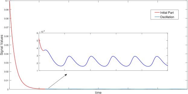
Refer to caption
Figure 24: Single regional-brain-activity signal generated by the structural connectivity matrices of Fig. 23 and model (20).

An example of the time series (yνt)tsubscriptsubscript𝑦𝜈𝑡𝑡(y_{\nu t})_{t}, for a single subject and a specific node, is shown in Fig. 24. As noted in the figure, there is an initial and an oscillation mode of the time series. Per node ν𝜈\nu, 500500500 samples from the initial phase and 500500500 ones from the oscillation phase of the signal comprise the time series (yνt)t=11,000superscriptsubscriptsubscript𝑦𝜈𝑡𝑡11000(y_{\nu t})_{t=1}^{1,000}. The sliding-window lengths τw{500,600,700,900}subscript𝜏w500600700900\tau_{\text{w}}\in\{500,600,700,900\} were tested. Length τw=700subscript𝜏w700\tau_{\text{w}}=700 produced better results than those of 500500500 and 600600600, for all clustering methods, while there was no significant improvement by setting τwsubscript𝜏w\tau_{\text{w}} equal to 900900900. For this reason, only results for τw=700subscript𝜏w700\tau_{\text{w}}=700 are shown here. As in Sec. V-A, both the methodologies of Secs. II and III are applied to this set of data, under choices of the linear, single Gaussian, and the multi-kernel functions, as well as the SDE approach. In the multi-kernel case, a weighted average of Gaussian kernels is used, i.e., κ:=(1/I)i=1Iκσiassign𝜅1𝐼superscriptsubscript𝑖1𝐼subscript𝜅subscript𝜎𝑖\kappa:=(1/I)\sum_{i=1}^{I}\kappa_{\sigma_{i}}, where σi{0.25+0.01(i1)}i=1Isubscript𝜎𝑖superscriptsubscript0.250.01𝑖1𝑖1𝐼\sigma_{i}\in\{0.25+0.01(i-1)\}_{i=1}^{I}, with I:=76assign𝐼76I:=76, σ1=0.25subscript𝜎10.25\sigma_{1}=0.25, and σI=1subscript𝜎𝐼1\sigma_{I}=1. Figs. 2529 show that GCT exhibits the most robust performance among all methods. The best clustering-accuracy result among Figs. 2529 is recorded for GCT in Fig. 25, with a value of 0.99970.99970.9997 for the “OB” feature.

Refer to caption
Figure 25: Linear kernel: NNNGCT=16superscriptsubscript𝑁NNGCT16N_{\text{NN}}^{\text{GCT}}=16.
Refer to caption
Figure 26: Single Gaussian kernel: σ2=0.5superscript𝜎20.5\sigma^{2}=0.5; NNNGCT=16superscriptsubscript𝑁NNGCT16N_{\text{NN}}^{\text{GCT}}=16.
Refer to caption
Figure 27: Single Gaussian kernel: σ2=1superscript𝜎21\sigma^{2}=1; NNNGCT=16superscriptsubscript𝑁NNGCT16N_{\text{NN}}^{\text{GCT}}=16.
Refer to caption
Figure 28: Multi-kernel: NNNGCT=16superscriptsubscript𝑁NNGCT16N_{\text{NN}}^{\text{GCT}}=16.
Refer to caption
Figure 29: SDE: NνtSDE=25subscriptsuperscript𝑁SDE𝜈𝑡25N^{\text{SDE}}_{\nu t}=25; N𝒢=83subscript𝑁𝒢83N_{\mathpzc{G}}=83; NNNGCT=16superscriptsubscript𝑁NNGCT16N_{\text{NN}}^{\text{GCT}}=16.

VI Conclusions and the Road Ahead

This paper introduced Riemannian multi-manifold modeling (RMMM) in the context of network-wide non-stationary time-series analysis. Features extracted sequentially from time series were used to define points in a Riemannian manifold, which under the RMMM hypothesis, are located in or close to a union of multiple Riemannian submanifolds. Two feature-generation mechanisms for network-wide time series were introduced: (i) Motivated by Granger-causality arguments, an auto-regressive moving average model was proposed to map low-rank linear vector subspaces, spanned by column vectors of appropriately defined observability matrices, to points into the Grassmann manifold; and (ii) to capture dynamic (non-linear) relations among nodes, kernel-based partial correlations were introduced to generate points in the manifold of positive-definite matrices. Furthermore, based on the very recent [79, 80], a clustering algorithm was introduced to segment the multiple Riemannian submanifolds which fit the data patterns. Extensive numerical tests demonstrated that the advocated framework outperforms classical and state-of-the-art techniques. On-going research focuses on (i) building an online spectral clustering scheme to alleviate the computational burden of Step 12 in Alg. 3; and (ii) applying the RMMM hypothesis to community detection scenarios, without any a-priori knowledge on the number of clusters.

Appendix A Reproducing Kernels

A real Hilbert space \mathpzc{H}, with elements denoted by f𝑓f and inner product |\langle\cdot\mathop{}|\mathop{}\cdot\rangle_{\mathpzc{H}}, is called a reproducing kernel Hilbert space (RKHS) [61, 7, 63] whenever, for an arbitrarily fixed row vector 𝒚τw𝒚superscriptsubscript𝜏w\bm{y}\in\mathbb{R}^{\tau_{\text{w}}}, the mapping ff(𝒚)maps-to𝑓𝑓𝒚f\mapsto f(\bm{y}) is continuous on \mathpzc{H}. This condition is equivalent to the existence of a (unique) reproducing kernel function κ(,):τw×τw:𝜅superscriptsubscript𝜏wsuperscriptsubscript𝜏w\kappa(\cdot,\cdot):\mathbb{R}^{\tau_{\text{w}}}\times\mathbb{R}^{\tau_{\text{w}}}\rightarrow\mathbb{R} which satisfies: (i) φ(𝒚):=κ(𝒚,)assign𝜑𝒚𝜅𝒚\varphi(\bm{y}):=\kappa(\bm{y},\cdot)\in\mathpzc{H}, 𝒚τwfor-all𝒚superscriptsubscript𝜏w\forall\bm{y}\in\mathbb{R}^{\tau_{\text{w}}}, and (ii) the following reproducing property holds: f(𝒚)=f|φ(𝒚)=f|κ(𝒚,)𝑓𝒚subscriptinner-product𝑓𝜑𝒚subscriptinner-product𝑓𝜅𝒚f(\bm{y})=\langle f\mathop{}|\mathop{}\varphi(\bm{y})\rangle_{\mathpzc{H}}=\langle f\mathop{}|\mathop{}\kappa(\bm{y},\cdot)\rangle_{\mathpzc{H}}, 𝒚τw,fformulae-sequencefor-all𝒚superscriptsubscript𝜏wfor-all𝑓\forall\bm{y}\in\mathbb{R}^{\tau_{\text{w}}},\forall f\in\mathpzc{H}. If f𝑓f is chosen to be κ(𝒚,)𝜅superscript𝒚\kappa(\bm{y}^{\prime},\cdot), then the previous reproducing property boils down to the so-called kernel trick: κ(𝒚,𝒚)=κ(𝒚,)|κ(𝒚,)𝜅superscript𝒚𝒚subscriptinner-product𝜅superscript𝒚𝜅𝒚\kappa(\bm{y}^{\prime},\bm{y})=\langle\kappa(\bm{y}^{\prime},\cdot)\mathop{}|\mathop{}\kappa(\bm{y},\cdot)\rangle_{\mathpzc{H}}, 𝒚,𝒚τwfor-all𝒚superscript𝒚superscriptsubscript𝜏w\forall\bm{y},\bm{y}^{\prime}\in\mathbb{R}^{\tau_{\text{w}}}. It turns out that =span¯{κ(y,):yτw}¯spanconditional-set𝜅yysuperscriptsubscript𝜏w\mathpzc{H}=\overline{\operatorname{span}}\{\kappa(\bm{y},\cdot):\bm{y}\in\mathbb{R}^{\tau_{\text{w}}}\}, where spanspan\operatorname{span} stands for the set of all linear combinations of the elements of a set, and the overline symbol denotes closure, in the strong-topology sense.

The previous definition has a more convenient algebraic characterization. Kernel κ𝜅\kappa is called positive definite if it is symmetric, i.e., κ(𝒚,𝒚)=κ(𝒚,𝒚)𝜅superscript𝒚𝒚𝜅𝒚superscript𝒚\kappa(\bm{y}^{\prime},\bm{y})=\kappa(\bm{y},\bm{y}^{\prime}), for any 𝒚,𝒚τw𝒚superscript𝒚superscriptsubscript𝜏w\bm{y},\bm{y}^{\prime}\in\mathbb{R}^{\tau_{\text{w}}}, and i=1Ij=1Iαiαjκ(𝒚i,𝒚j)0superscriptsubscript𝑖1𝐼superscriptsubscript𝑗1𝐼subscript𝛼𝑖subscript𝛼𝑗𝜅subscript𝒚𝑖subscript𝒚𝑗0\sum_{i=1}^{I}\sum_{j=1}^{I}\alpha_{i}\alpha_{j}\kappa(\bm{y}_{i},\bm{y}_{j})\geq 0, for any {αi}i=1Isuperscriptsubscriptsubscript𝛼𝑖𝑖1𝐼\{\alpha_{i}\}_{i=1}^{I}\subset\mathbb{R}, any {𝒚i}i=1Iτwsuperscriptsubscriptsubscript𝒚𝑖𝑖1𝐼superscriptsubscript𝜏w\{\bm{y}_{i}\}_{i=1}^{I}\subset\mathbb{R}^{\tau_{\text{w}}}, and any I>0𝐼subscriptabsent0I\in\mathbb{Z}_{>0}. The positive definiteness of κ𝜅\kappa can be stated equivalently via the property that the kernel matrix 𝐊𝐊\mathbf{K}, defined by [𝐊]ij:=κ(𝒚i,𝒚j)assignsubscriptdelimited-[]𝐊𝑖𝑗𝜅subscript𝒚𝑖subscript𝒚𝑗[\mathbf{K}]_{ij}:=\kappa(\bm{y}_{i},\bm{y}_{j}), is positive semidefinite, since ijαiαjκ(𝒚i,𝒚j)=𝜶𝐊𝜶subscript𝑖subscript𝑗subscript𝛼𝑖subscript𝛼𝑗𝜅subscript𝒚𝑖subscript𝒚𝑗superscript𝜶top𝐊𝜶\sum_{i}\sum_{j}\alpha_{i}\alpha_{j}\kappa(\bm{y}_{i},\bm{y}_{j})=\bm{\alpha}^{\top}\mathbf{K}\bm{\alpha}, for 𝜶:=[α1,,αI]assign𝜶superscriptsubscript𝛼1subscript𝛼𝐼top\bm{\alpha}:=[\alpha_{1},\ldots,\alpha_{I}]^{\top}. Remarkably, positive definiteness of a kernel characterizes its reproducing property. Indeed, the reproducing kernel κ𝜅\kappa of an RKHS \mathpzc{H} is positive definite [63], and given a positive definite kernel κ𝜅\kappa, there exists a unique RKHS \mathpzc{H} s.t. κ𝜅\kappa is the reproducing kernel of \mathpzc{H} [48].

Celebrated examples of reproducing kernels are the (i) linear kernel: κl(𝒚,𝒚):=𝒚𝒚\kappa_{\text{l}}(\bm{y},\bm{y}^{\prime}):=\bm{y}\bm{y}^{\prime}{}^{\top} (recall that 𝒚,𝒚𝒚superscript𝒚\bm{y},\bm{y}^{\prime} are row vectors). In this case, =τwsuperscriptsubscript𝜏w\mathpzc{H}=\mathbb{R}^{\tau_{\text{w}}}, φ(𝒚)=𝒚𝜑𝒚𝒚\varphi(\bm{y})=\bm{y}, and 𝐊=𝐘𝐘𝐊superscript𝐘𝐘top\mathbf{K}=\mathbf{Y}\mathbf{Y}^{\top}, where 𝐘𝐘\mathbf{Y} is the matrix whose rows are vectors {𝒚i}i=1Isuperscriptsubscriptsubscript𝒚𝑖𝑖1𝐼\{\bm{y}_{i}\}_{i=1}^{I}; (ii) polynomial kernel: κp(𝒚,𝒚):=(𝒚𝒚+1)q\kappa_{\text{p}}(\bm{y},\bm{y}^{\prime}):=(\bm{y}\bm{y}^{\prime}{}^{\top}+1)^{q}, where q>0𝑞subscriptabsent0q\in\mathbb{Z}_{>0}; and the (iii) Gaussian kernel: κσ(𝒚,𝒚):=exp[𝒚𝒚2/(2σ2)]assignsubscript𝜅𝜎𝒚superscript𝒚superscriptdelimited-∥∥𝒚superscript𝒚22superscript𝜎2\kappa_{\sigma}(\bm{y},\bm{y}^{\prime}):=\exp[-\lVert\bm{y}-\bm{y}^{\prime}\rVert^{2}/(2\sigma^{2})], for some σ>0𝜎subscriptabsent0\sigma\in\mathbb{R}_{>0}. It turns out that dimσ=+dimensionsubscript𝜎\dim\mathpzc{H}_{\sigma}=+\infty, e.g., [63].

Appendix B Logarithm Maps of Gr(mN𝒢,pρ)Gr𝑚subscript𝑁𝒢𝑝𝜌\text{Gr}(mN_{\mathpzc{G}},p\rho) and PD(N𝒢)PDsubscript𝑁𝒢\text{PD}(N_{\mathpzc{G}})

An efficient way to compute the logarithm map of the Grassmannian Gr(mN𝒢,pρ)Gr𝑚subscript𝑁𝒢𝑝𝜌\text{Gr}(mN_{\mathpzc{G}},p\rho), under a computational complexity of 𝒪(mN𝒢p2ρ2)𝒪𝑚subscript𝑁𝒢superscript𝑝2superscript𝜌2\mathcal{O}(mN_{\mathpzc{G}}p^{2}\rho^{2}), is provided in [25]. Per point xtsubscript𝑥𝑡x_{t} of Gr(mN𝒢,pρ)Gr𝑚subscript𝑁𝒢𝑝𝜌\text{Gr}(mN_{\mathpzc{G}},p\rho), [25] requires an mN𝒢×mN𝒢𝑚subscript𝑁𝒢𝑚subscript𝑁𝒢mN_{\mathpzc{G}}\times mN_{\mathpzc{G}} orthogonal matrix 𝐎𝐎\mathbf{O}, having its first pρ𝑝𝜌p\rho columns, denoted by the mN𝒢×pρ𝑚subscript𝑁𝒢𝑝𝜌mN_{\mathpzc{G}}\times p\rho matrix 𝐋𝐋\mathbf{L}, span the subspace xtsubscript𝑥𝑡x_{t}. Given xtsubscript𝑥𝑡x_{t} and xtsubscript𝑥superscript𝑡x_{t^{\prime}} of the Grassmannian, or equivalently, pairs (𝐎,𝐋𝐎𝐋\mathbf{O},\mathbf{L}) and (𝐎,𝐋superscript𝐎superscript𝐋\mathbf{O}^{\prime},\mathbf{L}^{\prime}), to compute logxt(xt)subscriptsubscript𝑥𝑡subscript𝑥superscript𝑡\log_{x_{t}}(x_{t^{\prime}}), the SVDs of 𝐋𝐋superscript𝐋topsuperscript𝐋\mathbf{L}^{\top}\mathbf{L}^{\prime} and 𝐎𝐋superscript𝐎topsuperscript𝐋\mathbf{O}^{\top}\mathbf{L}^{\prime} are needed.

Regarding manifold PD(N𝒢)PDsubscript𝑁𝒢\text{PD}(N_{\mathpzc{G}}), [76] computes logarithm log𝐌(𝐌)subscript𝐌superscript𝐌\log_{\mathbf{M}}(\mathbf{M}^{\prime}), 𝐌,𝐌PD(N𝒢)𝐌superscript𝐌PDsubscript𝑁𝒢\mathbf{M},\mathbf{M}^{\prime}\in\text{PD}(N_{\mathpzc{G}}), by first computing the Cholesky decomposition 𝐌=𝐆2𝐌superscript𝐆2\mathbf{M}=\mathbf{G}^{2}, for a symmetric 𝐆𝐆\mathbf{G}, and by forming log𝐌(𝐌)=𝐆log(𝐆1𝐌𝐆1)𝐆subscript𝐌superscript𝐌𝐆superscript𝐆1superscript𝐌superscript𝐆1𝐆\log_{\mathbf{M}}(\mathbf{M}^{\prime})=\mathbf{G}\log(\mathbf{G}^{-1}\mathbf{M}^{\prime}\mathbf{G}^{-1})\mathbf{G}, where log\log denotes the matrix logarithm, under overall complexity 𝒪(N𝒢3)𝒪superscriptsubscript𝑁𝒢3\mathcal{O}(N_{\mathpzc{G}}^{3}).

Appendix C Proof of Proposition 1

To reduce clutter, subscript t𝑡t will be dropped from all subsequent symbols. Moreover, 𝒚~ν:=𝒚~νtassignsubscript~𝒚𝜈subscript~𝒚𝜈𝑡\tilde{\bm{y}}_{\nu}:=\tilde{\bm{y}}_{\nu t}, 𝐘~12:=𝐘~12,tassignsubscript~𝐘12subscript~𝐘12𝑡\tilde{\mathbf{Y}}_{-12}:=\tilde{\mathbf{Y}}_{-12,t}, φν:=φ(𝒚~ν)assignsubscript𝜑𝜈𝜑subscript~𝒚𝜈\varphi_{\nu}:=\varphi(\tilde{\bm{y}}_{\nu}), and 𝝋12:=𝝋(𝐘~12)assignsubscript𝝋12𝝋subscript~𝐘12\bm{\varphi}_{-12}:=\bm{\varphi}(\tilde{\mathbf{Y}}_{-12}).

Assuming w.l.o.g. that i<j𝑖𝑗i<j, then there exists an N𝒢×N𝒢subscript𝑁𝒢subscript𝑁𝒢N_{\mathpzc{G}}\times N_{\mathpzc{G}} permutation matrix 𝐐𝐐\mathbf{Q} s.t.

Indeed, 𝐐𝐐\mathbf{Q} can be defined by swapping the 111st and i𝑖ith row, as well as the 222nd and j𝑗jth row of the identity matrix 𝐈N𝒢subscript𝐈subscript𝑁𝒢\mathbf{I}_{N_{\mathpzc{G}}}. According to (15a), 𝐊/𝐊ij=𝚷/𝐊ij=𝚷/𝚷22𝐊subscript𝐊𝑖𝑗𝚷subscript𝐊𝑖𝑗𝚷subscript𝚷22\mathbf{K}/\mathbf{K}_{-ij}=\bm{\Pi}/\mathbf{K}_{-ij}=\bm{\Pi}/\bm{\Pi}_{22}.

By standard arguments of LS estimation, for l{i,j}𝑙𝑖𝑗l\in\{i,j\},

𝜷^lsubscript^𝜷𝑙\displaystyle\hat{\bm{\beta}}_{l} argmin𝜷N𝒢2φl𝜷𝝋ij2\displaystyle\in\operatorname*{arg\,min}\nolimits_{\bm{\beta}\in\mathbb{R}^{N_{\mathpzc{G}}-2}}\,\left\lVert\varphi_{l}-\bm{\beta}\bm{\varphi}_{-{ij}}\right\rVert_{\mathpzc{H}}^{2}
=argmin𝜷φ(𝒚~l)ν𝒱𝒾𝒿βνφ(𝒚~ν)2\displaystyle=\operatorname*{arg\,min}\nolimits_{\bm{\beta}}\,\left\lVert\varphi(\tilde{\bm{y}}_{l})-\sum\nolimits_{\nu\in\mathpzc{V}_{-ij}}\beta_{\nu}\varphi(\tilde{\bm{y}}_{\nu})\right\rVert_{\mathpzc{H}}^{2} (21)

yields the orthogonal projection φ^l:=𝜷^l𝝋12assignsubscript^𝜑𝑙subscript^𝜷𝑙subscript𝝋12\hat{\varphi}_{l}:=\hat{\bm{\beta}}_{l}\bm{\varphi}_{-{12}} of φlsubscript𝜑𝑙\varphi_{l} onto the closed linear subspace spanned by {φν}ν𝒱𝒾𝒿subscriptsubscript𝜑𝜈𝜈subscript𝒱𝒾𝒿\{\varphi_{\nu}\}_{\nu\in\mathpzc{V}_{-ij}}. As such, 𝜷^lsubscript^𝜷𝑙\hat{\bm{\beta}}_{l} satisfies the normal equations 𝜷^l𝐊12=𝒌12,lsubscript^𝜷𝑙subscript𝐊12subscript𝒌12𝑙\hat{\bm{\beta}}_{l}\mathbf{K}_{-{12}}=\bm{k}_{-12,l}, since 𝐊12subscript𝐊12\mathbf{K}_{-{12}} in (12) is the Gram matrix formed by {φν}ν𝒱𝒾𝒿subscriptsubscript𝜑𝜈𝜈subscript𝒱𝒾𝒿\{\varphi_{\nu}\}_{\nu\in\mathpzc{V}_{-ij}}. Hence, the minimum-norm 𝜷^lsubscript^𝜷𝑙\hat{\bm{\beta}}_{l} of (21) can be obtained by 𝒌12,l𝐊12subscript𝒌12𝑙superscriptsubscript𝐊12\bm{k}_{-12,l}\mathbf{K}_{-{12}}^{\dagger}. Clearly, φ^l:=𝒌12,l𝐊12𝝋12assignsubscript^𝜑𝑙subscript𝒌12𝑙superscriptsubscript𝐊12subscript𝝋12\hat{\varphi}_{l}:=\bm{k}_{-12,l}\mathbf{K}_{-{12}}^{\dagger}\bm{\varphi}_{-{12}}, which justifies (13).

Now, it can be verified that

r~iκ|r~jκsubscriptinner-productsubscriptsubscript~𝑟𝑖𝜅subscriptsubscript~𝑟𝑗𝜅\displaystyle\left\langle\prescript{}{\kappa}{\tilde{r}}_{i}\mathop{}\middle|\mathop{}\prescript{}{\kappa}{\tilde{r}}_{j}\right\rangle_{\mathpzc{H}} =\displaystyle\,\mathbin{=}\, φiφ^i|φjφ^jsubscriptinner-productsubscript𝜑𝑖subscript^𝜑𝑖subscript𝜑𝑗subscript^𝜑𝑗\displaystyle\left\langle\varphi_{i}-\hat{\varphi}_{i}\mathop{}\middle|\mathop{}\varphi_{j}-\hat{\varphi}_{j}\right\rangle_{\mathpzc{H}}
=\displaystyle\,\mathbin{=}\, φiν𝒱𝒾𝒿[𝒌ij,i𝐊ij]νφν|brasubscript𝜑𝑖subscript𝜈subscript𝒱𝒾𝒿subscriptdelimited-[]subscript𝒌𝑖𝑗𝑖superscriptsubscript𝐊𝑖𝑗𝜈subscript𝜑𝜈\displaystyle\left\langle\left.{\varphi_{i}-\sum\nolimits_{\nu\in\mathpzc{V}_{-ij}}[\bm{k}_{-ij,i}\mathbf{K}_{-{ij}}^{\dagger}]_{\nu}\varphi_{\nu}}\right|\right.
φjν𝒱𝒾𝒿[𝒌ij,j𝐊ij]νφν\displaystyle\qquad\left.{\varphi_{j}-\sum\nolimits_{\nu^{\prime}\in\mathpzc{V}_{-ij}}[\bm{k}_{-ij,j}\mathbf{K}_{-{ij}}^{\dagger}]_{\nu^{\prime}}\varphi_{\nu^{\prime}}}\right\rangle_{\mathpzc{H}}
=\displaystyle\,\mathbin{=}\, φi|φj2𝒌ij,i𝐊ij𝒌ij,jsubscriptinner-productsubscript𝜑𝑖subscript𝜑𝑗2subscript𝒌𝑖𝑗𝑖superscriptsubscript𝐊𝑖𝑗superscriptsubscript𝒌𝑖𝑗𝑗top\displaystyle\langle\varphi_{i}\mathop{}|\mathop{}\varphi_{j}\rangle_{\mathpzc{H}}-2\bm{k}_{-ij,i}\mathbf{K}_{-{ij}}^{\dagger}\bm{k}_{-ij,j}^{\top}
+𝒌ij,1𝐊ij𝐊ij𝐊ij𝒌ij,jsubscript𝒌𝑖𝑗1superscriptsubscript𝐊𝑖𝑗subscript𝐊𝑖𝑗superscriptsubscript𝐊𝑖𝑗superscriptsubscript𝒌𝑖𝑗𝑗top\displaystyle+\bm{k}_{-ij,1}\mathbf{K}_{-{ij}}^{\dagger}\mathbf{K}_{-{ij}}\mathbf{K}_{-ij}^{\dagger}\bm{k}_{-ij,j}^{\top} (22a)
=\displaystyle\,\mathbin{=}\, φi|φj2𝒌ij,i𝐊ij𝒌ij,jsubscriptinner-productsubscript𝜑𝑖subscript𝜑𝑗2subscript𝒌𝑖𝑗𝑖superscriptsubscript𝐊𝑖𝑗superscriptsubscript𝒌𝑖𝑗𝑗top\displaystyle\langle\varphi_{i}\mathop{}|\mathop{}\varphi_{j}\rangle_{\mathpzc{H}}-2\bm{k}_{-ij,i}\mathbf{K}_{-{ij}}^{\dagger}\bm{k}_{-ij,j}^{\top}
+𝒌ij,i𝐊ij𝒌ij,jsubscript𝒌𝑖𝑗𝑖superscriptsubscript𝐊𝑖𝑗superscriptsubscript𝒌𝑖𝑗𝑗top\displaystyle+\bm{k}_{-ij,i}\mathbf{K}_{-{ij}}^{\dagger}\bm{k}_{-ij,j}^{\top} (22b)
=\displaystyle\,\mathbin{=}\, φi|φj𝒌ij,i𝐊ij𝒌ij,jsubscriptinner-productsubscript𝜑𝑖subscript𝜑𝑗subscript𝒌𝑖𝑗𝑖superscriptsubscript𝐊𝑖𝑗superscriptsubscript𝒌𝑖𝑗𝑗top\displaystyle\langle\varphi_{i}\mathop{}|\mathop{}\varphi_{j}\rangle_{\mathpzc{H}}-\bm{k}_{-ij,i}\mathbf{K}_{-{ij}}^{\dagger}\bm{k}_{-ij,j}^{\top}
=\displaystyle\,\mathbin{=}\, [𝚷/𝚷22]12,subscriptdelimited-[]𝚷subscript𝚷2212\displaystyle[\bm{\Pi}/\bm{\Pi}_{22}]_{12}\,, (22c)

where the linearity of the inner product was used in (22a), and the properties of the Moore-Penrose pseudoinverse in (22b). In a similar way to (22), it can be verified that

r~lκ2subscriptsuperscriptdelimited-∥∥subscriptsubscript~𝑟𝑙𝜅2\displaystyle\left\lVert\prescript{}{\kappa}{\tilde{r}}_{l}\right\rVert^{2}_{\mathpzc{H}} =φlφ^l2=φl2𝒌ij,l𝐊ij𝒌ij,labsentsubscriptsuperscriptdelimited-∥∥subscript𝜑𝑙subscript^𝜑𝑙2subscriptsuperscriptdelimited-∥∥subscript𝜑𝑙2subscript𝒌𝑖𝑗𝑙superscriptsubscript𝐊𝑖𝑗superscriptsubscript𝒌𝑖𝑗𝑙top\displaystyle=\left\lVert\varphi_{l}-\hat{\varphi}_{l}\right\rVert^{2}_{\mathpzc{H}}=\lVert\varphi_{l}\rVert^{2}_{\mathpzc{H}}-\bm{k}_{-ij,l}\mathbf{K}_{-{ij}}^{\dagger}\bm{k}_{-ij,l}^{\top}
=[𝚷/𝚷22]ll,l{1,2}.formulae-sequenceabsentsubscriptdelimited-[]𝚷subscript𝚷22𝑙𝑙𝑙12\displaystyle=[\bm{\Pi}/\bm{\Pi}_{22}]_{ll}\,,\quad l\in\{1,2\}\,. (23)

Hence, (15b) follows from (22c) and (23).

If 𝐊𝟎succeeds𝐊0\mathbf{K}\succ\mathbf{0}, then also 𝚷𝟎succeeds𝚷0\bm{\Pi}\succ\mathbf{0}. This implies that 𝐊ij=𝚷22𝟎subscript𝐊𝑖𝑗subscript𝚷22succeeds0\mathbf{K}_{-ij}=\bm{\Pi}_{22}\succ\mathbf{0}, 𝚷110succeedssubscript𝚷110\bm{\Pi}_{11}\succ 0, 𝚷/𝚷22𝟎succeeds𝚷subscript𝚷220\bm{\Pi}/\bm{\Pi}_{22}\succ\mathbf{0}, and 𝚷/𝚷11𝟎succeeds𝚷subscript𝚷110\bm{\Pi}/\bm{\Pi}_{11}\succ\mathbf{0} [10, 3]. Consequently, 𝐊12=𝐊121superscriptsubscript𝐊12superscriptsubscript𝐊121\mathbf{K}_{-{12}}^{\dagger}=\mathbf{K}_{-{12}}^{-1} [10]. If 𝚵:=[ξll]:=(𝚷/𝚷22)1assign𝚵delimited-[]subscript𝜉𝑙superscript𝑙assignsuperscript𝚷subscript𝚷221\bm{\Xi}:=[\xi_{ll^{\prime}}]:=(\bm{\Pi}/\bm{\Pi}_{22})^{-1}, and if Minorll()subscriptMinor𝑙superscript𝑙\operatorname{Minor}_{ll^{\prime}}(\cdot) stands for the (l,l)𝑙superscript𝑙(l,l^{\prime})th minor of a square matrix, Cramer’s rule dictates that [𝚵1]ll=(1/det𝚵)(1)l+lMinorll(𝚵)subscriptdelimited-[]superscript𝚵1𝑙superscript𝑙1𝚵superscript1𝑙superscript𝑙subscriptMinorsuperscript𝑙𝑙𝚵[\bm{\Xi}^{-1}]_{ll^{\prime}}=(1/\det\bm{\Xi})\cdot(-1)^{l+l^{\prime}}\cdot\operatorname{Minor}_{l^{\prime}l}(\bm{\Xi}). Recall also the well-known fact [10, p. 30]:

𝚷1=[(𝚷/𝚷22)1𝚷111𝚷12(𝚷/𝚷11)1𝚷221𝚷21(𝚷/𝚷22)1(𝚷/𝚷11)1],superscript𝚷1matrixsuperscript𝚷subscript𝚷221superscriptsubscript𝚷111subscript𝚷12superscript𝚷subscript𝚷111superscriptsubscript𝚷221subscript𝚷21superscript𝚷subscript𝚷221superscript𝚷subscript𝚷111\displaystyle\bm{\Pi}^{-1}=\begin{bmatrix}(\bm{\Pi}/\bm{\Pi}_{22})^{-1}&-\bm{\Pi}_{11}^{-1}\bm{\Pi}_{12}(\bm{\Pi}/\bm{\Pi}_{11})^{-1}\\ -\bm{\Pi}_{22}^{-1}\bm{\Pi}_{21}(\bm{\Pi}/\bm{\Pi}_{22})^{-1}&(\bm{\Pi}/\bm{\Pi}_{11})^{-1}\end{bmatrix}\,,

which suggests that 𝚵𝚵\bm{\Xi} is the 2×2222\times 2 upper-left submatrix of 𝚷1superscript𝚷1\bm{\Pi}^{-1}. By (15b), (15c) is established as follows:

ϱ^ijκsubscriptsubscript^italic-ϱ𝑖𝑗𝜅\displaystyle\prescript{}{\kappa}{\hat{\varrho}}_{ij} =[𝐊/𝐊ij]12[𝐊/𝐊ij]11[𝐊/𝐊ij]22 absentsubscriptdelimited-[]𝐊superscript𝐊𝑖𝑗12[𝐊/𝐊ij]11[𝐊/𝐊ij]22 \displaystyle=\frac{[\mathbf{K}/\mathbf{K}^{-ij}]_{12}}{\mathchoice{{\hbox{$\displaystyle\sqrt{[\mathbf{K}/\mathbf{K}_{-ij}]_{11}\cdot[\mathbf{K}/\mathbf{K}_{-ij}]_{22}\,}$}\lower 0.4pt\hbox{\vrule height=7.5pt,depth=-6.00003pt}}}{{\hbox{$\textstyle\sqrt{[\mathbf{K}/\mathbf{K}_{-ij}]_{11}\cdot[\mathbf{K}/\mathbf{K}_{-ij}]_{22}\,}$}\lower 0.4pt\hbox{\vrule height=7.5pt,depth=-6.00003pt}}}{{\hbox{$\scriptstyle\sqrt{[\mathbf{K}/\mathbf{K}_{-ij}]_{11}\cdot[\mathbf{K}/\mathbf{K}_{-ij}]_{22}\,}$}\lower 0.4pt\hbox{\vrule height=5.25pt,depth=-4.20003pt}}}{{\hbox{$\scriptscriptstyle\sqrt{[\mathbf{K}/\mathbf{K}_{-ij}]_{11}\cdot[\mathbf{K}/\mathbf{K}_{-ij}]_{22}\,}$}\lower 0.4pt\hbox{\vrule height=3.75pt,depth=-3.00002pt}}}}
=[𝚷/𝚷22]12[𝚷/𝚷22]11[𝚷/𝚷22]22 =[𝚵1]12[𝚵1]11[𝚵1]22 absentsubscriptdelimited-[]𝚷subscript𝚷2212[𝚷/𝚷22]11[𝚷/𝚷22]22 subscriptdelimited-[]superscript𝚵112[𝚵1]11[𝚵1]22 \displaystyle=\frac{[\bm{\Pi}/\bm{\Pi}_{22}]_{12}}{\mathchoice{{\hbox{$\displaystyle\sqrt{[\bm{\Pi}/\bm{\Pi}_{22}]_{11}\cdot[\bm{\Pi}/\bm{\Pi}_{22}]_{22}\,}$}\lower 0.4pt\hbox{\vrule height=7.5pt,depth=-6.00003pt}}}{{\hbox{$\textstyle\sqrt{[\bm{\Pi}/\bm{\Pi}_{22}]_{11}\cdot[\bm{\Pi}/\bm{\Pi}_{22}]_{22}\,}$}\lower 0.4pt\hbox{\vrule height=7.5pt,depth=-6.00003pt}}}{{\hbox{$\scriptstyle\sqrt{[\bm{\Pi}/\bm{\Pi}_{22}]_{11}\cdot[\bm{\Pi}/\bm{\Pi}_{22}]_{22}\,}$}\lower 0.4pt\hbox{\vrule height=5.25pt,depth=-4.20003pt}}}{{\hbox{$\scriptscriptstyle\sqrt{[\bm{\Pi}/\bm{\Pi}_{22}]_{11}\cdot[\bm{\Pi}/\bm{\Pi}_{22}]_{22}\,}$}\lower 0.4pt\hbox{\vrule height=3.75pt,depth=-3.00002pt}}}}=\frac{[\bm{\Xi}^{-1}]_{12}}{\mathchoice{{\hbox{$\displaystyle\sqrt{[\bm{\Xi}^{-1}]_{11}\cdot[\bm{\Xi}^{-1}]_{22}\,}$}\lower 0.4pt\hbox{\vrule height=8.63776pt,depth=-6.91023pt}}}{{\hbox{$\textstyle\sqrt{[\bm{\Xi}^{-1}]_{11}\cdot[\bm{\Xi}^{-1}]_{22}\,}$}\lower 0.4pt\hbox{\vrule height=8.63776pt,depth=-6.91023pt}}}{{\hbox{$\scriptstyle\sqrt{[\bm{\Xi}^{-1}]_{11}\cdot[\bm{\Xi}^{-1}]_{22}\,}$}\lower 0.4pt\hbox{\vrule height=6.0722pt,depth=-4.85779pt}}}{{\hbox{$\scriptscriptstyle\sqrt{[\bm{\Xi}^{-1}]_{11}\cdot[\bm{\Xi}^{-1}]_{22}\,}$}\lower 0.4pt\hbox{\vrule height=4.70554pt,depth=-3.76445pt}}}}
=(1)1+2Minor21(𝚵)[(1)1+1Minor11(𝚵)(1)2+2Minor22(𝚵)]1/2absentsuperscript112subscriptMinor21𝚵superscriptdelimited-[]superscript111subscriptMinor11𝚵superscript122subscriptMinor22𝚵12\displaystyle=\frac{(-1)^{1+2}\cdot\operatorname{Minor}_{21}(\bm{\Xi})}{\left[(-1)^{1+1}\operatorname{Minor}_{11}(\bm{\Xi})\cdot(-1)^{2+2}\operatorname{Minor}_{22}(\bm{\Xi})\right]^{1/2}}
=ξ12ξ22ξ11 =[𝚷1]12[𝚷1]22[𝚷1]11 absentsubscript𝜉12ξ22ξ11 subscriptdelimited-[]superscript𝚷112[𝚷1]22[𝚷1]11 \displaystyle=\frac{-\xi_{12}}{\mathchoice{{\hbox{$\displaystyle\sqrt{\xi_{22}\xi_{11}\,}$}\lower 0.4pt\hbox{\vrule height=6.94444pt,depth=-5.55559pt}}}{{\hbox{$\textstyle\sqrt{\xi_{22}\xi_{11}\,}$}\lower 0.4pt\hbox{\vrule height=6.94444pt,depth=-5.55559pt}}}{{\hbox{$\scriptstyle\sqrt{\xi_{22}\xi_{11}\,}$}\lower 0.4pt\hbox{\vrule height=4.8611pt,depth=-3.8889pt}}}{{\hbox{$\scriptscriptstyle\sqrt{\xi_{22}\xi_{11}\,}$}\lower 0.4pt\hbox{\vrule height=3.47221pt,depth=-2.77779pt}}}}=\frac{-[\bm{\Pi}^{-1}]_{12}}{\mathchoice{{\hbox{$\displaystyle\sqrt{[\bm{\Pi}^{-1}]_{22}\cdot[\bm{\Pi}^{-1}]_{11}\,}$}\lower 0.4pt\hbox{\vrule height=8.63776pt,depth=-6.91023pt}}}{{\hbox{$\textstyle\sqrt{[\bm{\Pi}^{-1}]_{22}\cdot[\bm{\Pi}^{-1}]_{11}\,}$}\lower 0.4pt\hbox{\vrule height=8.63776pt,depth=-6.91023pt}}}{{\hbox{$\scriptstyle\sqrt{[\bm{\Pi}^{-1}]_{22}\cdot[\bm{\Pi}^{-1}]_{11}\,}$}\lower 0.4pt\hbox{\vrule height=6.0722pt,depth=-4.85779pt}}}{{\hbox{$\scriptscriptstyle\sqrt{[\bm{\Pi}^{-1}]_{22}\cdot[\bm{\Pi}^{-1}]_{11}\,}$}\lower 0.4pt\hbox{\vrule height=4.70554pt,depth=-3.76445pt}}}}
=[𝐐𝐊1𝐐]12[𝐐𝐊1𝐐]11[𝐐𝐊1𝐐]22 absentsubscriptdelimited-[]superscript𝐐𝐊1superscript𝐐top12[𝐐𝐊1𝐐]11[𝐐𝐊1𝐐]22 \displaystyle=\frac{-[\mathbf{Q}\mathbf{K}^{-1}\mathbf{Q}^{\top}]_{12}}{\mathchoice{{\hbox{$\displaystyle\sqrt{[\mathbf{Q}\mathbf{K}^{-1}\mathbf{Q}^{\top}]_{11}\cdot[\mathbf{Q}\mathbf{K}^{-1}\mathbf{Q}^{\top}]_{22}\,}$}\lower 0.4pt\hbox{\vrule height=8.77776pt,depth=-7.02223pt}}}{{\hbox{$\textstyle\sqrt{[\mathbf{Q}\mathbf{K}^{-1}\mathbf{Q}^{\top}]_{11}\cdot[\mathbf{Q}\mathbf{K}^{-1}\mathbf{Q}^{\top}]_{22}\,}$}\lower 0.4pt\hbox{\vrule height=8.77776pt,depth=-7.02223pt}}}{{\hbox{$\scriptstyle\sqrt{[\mathbf{Q}\mathbf{K}^{-1}\mathbf{Q}^{\top}]_{11}\cdot[\mathbf{Q}\mathbf{K}^{-1}\mathbf{Q}^{\top}]_{22}\,}$}\lower 0.4pt\hbox{\vrule height=6.17221pt,depth=-4.93779pt}}}{{\hbox{$\scriptscriptstyle\sqrt{[\mathbf{Q}\mathbf{K}^{-1}\mathbf{Q}^{\top}]_{11}\cdot[\mathbf{Q}\mathbf{K}^{-1}\mathbf{Q}^{\top}]_{22}\,}$}\lower 0.4pt\hbox{\vrule height=4.80554pt,depth=-3.84445pt}}}}
=[𝐊1]ij[𝐊1]ii[𝐊1]jj .absentsubscriptdelimited-[]superscript𝐊1𝑖𝑗[𝐊1]ii[𝐊1]jj \displaystyle=\frac{-[\mathbf{K}^{-1}]_{ij}}{\mathchoice{{\hbox{$\displaystyle\sqrt{[\mathbf{K}^{-1}]_{ii}\cdot[\mathbf{K}^{-1}]_{jj}\,}$}\lower 0.4pt\hbox{\vrule height=8.63776pt,depth=-6.91023pt}}}{{\hbox{$\textstyle\sqrt{[\mathbf{K}^{-1}]_{ii}\cdot[\mathbf{K}^{-1}]_{jj}\,}$}\lower 0.4pt\hbox{\vrule height=8.63776pt,depth=-6.91023pt}}}{{\hbox{$\scriptstyle\sqrt{[\mathbf{K}^{-1}]_{ii}\cdot[\mathbf{K}^{-1}]_{jj}\,}$}\lower 0.4pt\hbox{\vrule height=6.0722pt,depth=-4.85779pt}}}{{\hbox{$\scriptscriptstyle\sqrt{[\mathbf{K}^{-1}]_{ii}\cdot[\mathbf{K}^{-1}]_{jj}\,}$}\lower 0.4pt\hbox{\vrule height=4.70554pt,depth=-3.76445pt}}}}\,.

Appendix D Semidefinite Embedding

Along the lines of the discussion in Appendix A, it is likely that the geometry of {𝒚~νt}subscript~𝒚𝜈𝑡\{\tilde{\bm{y}}_{\nu t}\} is “destroyed” during the transfer {𝒚~νt}{φ(𝒚~νt)}maps-tosubscript~𝒚𝜈𝑡𝜑subscript~𝒚𝜈𝑡\{\tilde{\bm{y}}_{\nu t}\}\mapsto\{\varphi(\tilde{\bm{y}}_{\nu t})\}, if no constraints are imposed on φ𝜑\varphi. To this end, the geometry of {𝒚~νt}subscript~𝒚𝜈𝑡\{\tilde{\bm{y}}_{\nu t}\} needs to be learned first. A graph is built on {𝒚~νt}subscript~𝒚𝜈𝑡\{\tilde{\bm{y}}_{\nu t}\}, and a weighted adjacency matrix 𝛀tsubscript𝛀𝑡\bm{\Omega}_{t}, as well as neighborhoods {𝒩νtSDE}ν=1N𝒢superscriptsubscriptsubscriptsuperscript𝒩SDE𝜈𝑡𝜈1subscript𝑁𝒢\{\mathcal{N}^{\text{SDE}}_{\nu t}\}_{\nu=1}^{N_{\mathpzc{G}}} are constructed. A straightforward way is: (i) Per node ν𝜈\nu, gather in 𝒩νtSDEsubscriptsuperscript𝒩SDE𝜈𝑡\mathcal{N}^{\text{SDE}}_{\nu t} the (user-defined) P>0𝑃subscriptabsent0P\in\mathbb{Z}_{>0} nearest neighbors (in a Euclidean-distance sense, for example) of 𝒚~νtsubscript~𝒚𝜈𝑡\tilde{\bm{y}}_{\nu t} among {𝒚~νt}ννsubscriptsubscript~𝒚superscript𝜈𝑡superscript𝜈𝜈\{\tilde{\bm{y}}_{\nu^{\prime}t}\}_{\nu^{\prime}\neq\nu}, including also 𝒚~νtsubscript~𝒚𝜈𝑡\tilde{\bm{y}}_{\nu t}; (ii) define 𝛀t:=[ωνν,t]assignsubscript𝛀𝑡delimited-[]subscript𝜔𝜈superscript𝜈𝑡\bm{\Omega}_{t}:=[\omega_{\nu\nu^{\prime},t}] as follows: wνν,t:=1/Passignsubscript𝑤𝜈superscript𝜈𝑡1𝑃w_{\nu\nu^{\prime},t}:=1/P, if 𝒚~νt𝒩νtSDEsubscript~𝒚superscript𝜈𝑡subscriptsuperscript𝒩SDE𝜈𝑡\tilde{\bm{y}}_{\nu^{\prime}t}\in\mathcal{N}^{\text{SDE}}_{\nu t}, and wνν:=0assignsubscript𝑤𝜈superscript𝜈0w_{\nu\nu^{\prime}}:=0, otherwise. Clearly, data vectors 𝒚~νtsubscript~𝒚𝜈𝑡\tilde{\bm{y}}_{\nu t} and 𝒚~νtsubscript~𝒚superscript𝜈𝑡\tilde{\bm{y}}_{\nu^{\prime}t} belong to the same neighborhood iff there exists ν′′superscript𝜈′′\nu^{\prime\prime} s.t. 𝒚~νt,𝒚~νt𝒩ν′′tSDEsubscript~𝒚𝜈𝑡subscript~𝒚superscript𝜈𝑡subscriptsuperscript𝒩SDEsuperscript𝜈′′𝑡\tilde{\bm{y}}_{\nu t},\tilde{\bm{y}}_{\nu^{\prime}t}\in\mathcal{N}^{\text{SDE}}_{\nu^{\prime\prime}t} iff ν′′superscript𝜈′′\exists\nu^{\prime\prime} with ων′′ν,tων′′ν,t>0subscript𝜔superscript𝜈′′𝜈𝑡subscript𝜔superscript𝜈′′superscript𝜈𝑡0\omega_{\nu^{\prime\prime}\nu,t}\cdot\omega_{\nu^{\prime\prime}\nu^{\prime},t}>0.

SDE postulates that data geometry, at least within neighborhoods defined via the previous step (i), should be preserved even after mapping data into \mathpzc{H}. For neighbors 𝒚~νt,𝒚~νtsubscript~𝒚𝜈𝑡subscript~𝒚superscript𝜈𝑡\tilde{\bm{y}}_{\nu t},\tilde{\bm{y}}_{\nu^{\prime}t}, distances should satisfy the isometric condition: φ(𝒚~νt)φ(𝒚~νt)2=𝒚~νt𝒚~νt22superscriptsubscriptdelimited-∥∥𝜑subscript~𝒚𝜈𝑡𝜑subscript~𝒚superscript𝜈𝑡2subscriptsuperscriptdelimited-∥∥subscript~𝒚𝜈𝑡subscript~𝒚superscript𝜈𝑡22\lVert\varphi(\tilde{\bm{y}}_{\nu t})-\varphi(\tilde{\bm{y}}_{\nu^{\prime}t})\rVert_{\mathpzc{H}}^{2}=\lVert\tilde{\bm{y}}_{\nu t}-\tilde{\bm{y}}_{\nu^{\prime}t}\rVert^{2}_{2}. By the kernel trick, the previous constraint translates to [𝐊t]νν2[𝐊t]νν+[𝐊t]νν=𝒚~νt𝒚~νt22subscriptdelimited-[]subscript𝐊𝑡𝜈𝜈2subscriptdelimited-[]subscript𝐊𝑡𝜈superscript𝜈subscriptdelimited-[]subscript𝐊𝑡superscript𝜈superscript𝜈subscriptsuperscriptdelimited-∥∥subscript~𝒚𝜈𝑡subscript~𝒚superscript𝜈𝑡22[\mathbf{K}_{t}]_{\nu\nu}-2[\mathbf{K}_{t}]_{\nu\nu^{\prime}}+[\mathbf{K}_{t}]_{\nu^{\prime}\nu^{\prime}}=\lVert\tilde{\bm{y}}_{\nu t}-\tilde{\bm{y}}_{\nu^{\prime}t}\rVert^{2}_{2}. Moreover, data are required to be “centered” around 00, i.e., ν=1N𝒢φ(𝒚~νt)=0superscriptsubscript𝜈1subscript𝑁𝒢𝜑subscript~𝒚𝜈𝑡0\sum_{\nu=1}^{N_{\mathpzc{G}}}\varphi(\tilde{\bm{y}}_{\nu t})=0. Again, by the kernel trick, νφ(𝒚~νt)=0νφ(𝒚~νt)|νφ(𝒚~νt)=0νν[𝐊t]νν=0subscript𝜈𝜑subscript~𝒚𝜈𝑡0subscriptinner-productsubscript𝜈𝜑subscript~𝒚𝜈𝑡subscriptsuperscript𝜈𝜑subscript~𝒚superscript𝜈𝑡0subscript𝜈subscriptsuperscript𝜈subscriptdelimited-[]subscript𝐊𝑡𝜈superscript𝜈0\sum_{\nu}\varphi(\tilde{\bm{y}}_{\nu t})=0\Leftrightarrow\langle\sum_{\nu}\varphi(\tilde{\bm{y}}_{\nu t})\mathop{}|\mathop{}\sum_{\nu^{\prime}}\varphi(\tilde{\bm{y}}_{\nu^{\prime}t})\rangle_{\mathpzc{H}}=0\Leftrightarrow\sum_{\nu}\sum_{\nu^{\prime}}[\mathbf{K}_{t}]_{\nu\nu^{\prime}}=0. Finally, the data cloud {φ(𝒚~νt)}t=1Tsuperscriptsubscript𝜑subscript~𝒚𝜈𝑡𝑡1𝑇\{\varphi(\tilde{\bm{y}}_{\nu t})\}_{t=1}^{T} should occupy “as much space as possible” within \mathpzc{H}. This can be achieved by the maximization of the “sample variance,” which, according to the previous constraints, becomes: ν=1N𝒢φ(𝒚~νt)(1/N𝒢)ν=1N𝒢φ(𝒚~νt)2=ν=1N𝒢φ(𝒚~νt)2=ν=1N𝒢φ(𝒚~νt)|φ(𝒚~νt)=ν=1N𝒢κ(𝒚~νt,𝒚~νt)=trace(𝐊t)superscriptsubscript𝜈1subscript𝑁𝒢subscriptsuperscriptdelimited-∥∥𝜑subscript~𝒚𝜈𝑡1subscript𝑁𝒢superscriptsubscriptsuperscript𝜈1subscript𝑁𝒢𝜑subscript~𝒚superscript𝜈𝑡2superscriptsubscript𝜈1subscript𝑁𝒢subscriptsuperscriptdelimited-∥∥𝜑subscript~𝒚𝜈𝑡2superscriptsubscript𝜈1subscript𝑁𝒢subscriptinner-product𝜑subscript~𝒚𝜈𝑡𝜑subscript~𝒚𝜈𝑡superscriptsubscript𝜈1subscript𝑁𝒢𝜅subscript~𝒚𝜈𝑡subscript~𝒚𝜈𝑡tracesubscript𝐊𝑡\sum_{\nu=1}^{N_{\mathpzc{G}}}\lVert\varphi(\tilde{\bm{y}}_{\nu t})-(1/N_{\mathpzc{G}})\sum_{\nu^{\prime}=1}^{N_{\mathpzc{G}}}\varphi(\tilde{\bm{y}}_{\nu^{\prime}t})\rVert^{2}_{\mathpzc{H}}=\sum_{\nu=1}^{N_{\mathpzc{G}}}\lVert\varphi(\tilde{\bm{y}}_{\nu t})\rVert^{2}_{\mathpzc{H}}=\sum_{\nu=1}^{N_{\mathpzc{G}}}\langle\varphi(\tilde{\bm{y}}_{\nu t})\mathop{}|\mathop{}\varphi(\tilde{\bm{y}}_{\nu t})\rangle_{\mathpzc{H}}=\sum_{\nu=1}^{N_{\mathpzc{G}}}\kappa(\tilde{\bm{y}}_{\nu t},\tilde{\bm{y}}_{\nu t})=\operatorname{trace}(\mathbf{K}_{t}).

SDE is posed as the following linear (convex) programming task over the set of PSD matrices: given data {𝒚~νt}ν=1N𝒢superscriptsubscriptsubscript~𝒚𝜈𝑡𝜈1subscript𝑁𝒢\{\tilde{\bm{y}}_{\nu t}\}_{\nu=1}^{N_{\mathpzc{G}}} per t𝑡t, as well as the weighted adjacency matrix 𝛀tsubscript𝛀𝑡\bm{\Omega}_{t}, find

𝐊tsubscript𝐊𝑡absent\displaystyle\mathbf{K}_{t}\in argmax𝐊trace(𝐊)subscript𝐊trace𝐊\displaystyle\arg\max\nolimits_{\mathbf{K}}\operatorname{trace}(\mathbf{K})
s.to[𝐊𝟎,ν=1N𝒢ν=1N𝒢[𝐊]νν=0,[[𝐊]νν2[𝐊]νν+[𝐊]νν=𝒚~νt𝒚~νt22,(ν,ν)s.t.ν′′withων′′ν,tων′′ν,t>0.\displaystyle\text{s.to}\ \left[\begin{aligned} &\mathbf{K}\succeq\mathbf{0}\,,\\ &\sum\nolimits_{\nu=1}^{N_{\mathpzc{G}}}\sum\nolimits_{\nu^{\prime}=1}^{N_{\mathpzc{G}}}[\mathbf{K}]_{\nu\nu^{\prime}}=0\,,\\ &\left[\begin{aligned} &[\mathbf{K}]_{\nu\nu}-2[\mathbf{K}]_{\nu\nu^{\prime}}+[\mathbf{K}]_{\nu^{\prime}\nu^{\prime}}=\lVert\tilde{\bm{y}}_{\nu t}-\tilde{\bm{y}}_{\nu^{\prime}t}\rVert^{2}_{2}\,,\\ &\forall(\nu,\nu^{\prime})\ \text{s.t.}\ \exists\nu^{\prime\prime}\ \text{with}\ \omega_{\nu^{\prime\prime}\nu,t}\cdot\omega_{\nu^{\prime\prime}\nu^{\prime},t}>0\,.\end{aligned}\right.\end{aligned}\right.

References

  • [1] G. Aggarwal, A. Roy-Chowdhury, and R. Chellappa, “A system identification approach for video-based face recognition,” in Proc. ICPR, Cambridge: UK, Aug. 2004.
  • [2] S. Aghabozorgi, A. S. Shirkhorshidi, and T. Y. Wah, “Time-series clustering — A decade review,” Information Systems, vol. 53, pp. 16–38, 2015.
  • [3] A. Albert, “Conditions for positive and nonnegative definiteness in terms of pseudoinverses,” SIAM J. Appl. Math., vol. 17, pp. 434–440, 1969.
  • [4] E. A. Allen, E. Damaraju, S. M. Plis, E. B. Erhardt, T. Eichele, and V. D. Calhoun, “Tracking whole-brain connectivity dynamics in the resting state,” Cerebral Cortex, vol. 24, pp. 663–676, 2014.
  • [5] E. Arias-Castro, G. Chen, and G. Lerman, “Spectral clustering based on local linear approximations,” Electron. J. Statist., vol. 5, pp. 1537–1587, 2011.
  • [6] E. Arias-Castro, G. Lerman, and T. Zhang, “Spectral clustering based on local PCA,” arXiv e-prints, 2013.
  • [7] N. Aronszajn, “Theory of reproducing kernels,” Trans. American Mathematical Society, vol. 68, no. 3, pp. 337–404, 1950.
  • [8] R. Basri, T. Hassner, and L. Zelnik-Manor, “Approximate nearest subspace search,” IEEE Trans. Pattern Analysis Machine Intell., vol. 33, no. 2, pp. 266–278, 2011.
  • [9] H. H. Bauschke and P. L. Combettes, Convex Analysis and Monotone Operator Theory in Hilbert Spaces.   New York: Springer, 2011.
  • [10] A. Ben-Israel and T. N. E. Greville, Generalized Inverses: Theory and Applications, 2nd ed.   New York: Springer-Verlag, 2003.
  • [11] H. Boudjellaba, J.-M. Dufour, and R. Roy, “Testing causality between two vectors in multivariate autoregressive moving average models,” J. American Statistical Assoc., vol. 87, no. 420, pp. 1082–1090, 1992.
  • [12] U. Braun, S. F. Muldoon, and D. S. Bassett, “On human brain networks in health and disease,” eLS, 2015.
  • [13] J. Britz, D. Van De Ville, and C. M. Michel, “BOLD correlates of EEG topography reveal rapid resting-state network dynamics,” NeuroImage, vol. 52, pp. 1162–1170, 2010.
  • [14] S. J. Broyd, C. Demanuele, S. Debener, S. K. Helps, C. J. James, and E. J. Sonuga-Barke, “Default-mode brain dysfunction in mental disorders: A systematic review,” Neuroscience & Biobehavioral Reviews, vol. 33, no. 3, pp. 279–296, 2009.
  • [15] R. L. Buckner and J. L. Vincent, “Unrest at rest: Default activity and spontaneous network correlations,” NeuroImage, vol. 37, no. 4, pp. 1091–1096, 2007.
  • [16] E. Bullmore and O. Sporns, “Complex brain networks: Graph theoretical analysis of structural and functional systems,” Nature Reviews Neuroscience, vol. 10, no. 3, pp. 186–198, 2009.
  • [17] V. D. Calhoun, R. Miller, G. Pearlson, and T. Adali, “The chronnectome: Time-varying connectivity networks as the next frontier in fMRI data discovery,” Neuron, vol. 84, pp. 262–274, Oct. 2014.
  • [18] H. Cetingul and R. Vidal, “Intrinsic mean shift for clustering on Stiefel and Grassmann manifolds,” in Proc. CVPR, June 2009, pp. 1896–1902.
  • [19] H. Cetingul, M. J. Wright, P. M. Thompson, and R. Vidal, “Segmentation of high angular resolution diffusion MRI using sparse Riemannian manifold clustering,” IEEE Trans. Medical Imag., vol. 33, no. 2, pp. 301–317, Feb. 2014.
  • [20] G. Chen and G. Lerman, “Foundations of a multi-way spectral clustering framework for hybrid linear modeling,” Found. Comput. Math., vol. 9, no. 5, pp. 517–558, 2009.
  • [21] Y. Chen, S. L. Bressler, and M. Ding, “Frequency decomposition of conditional Granger causality and application to multivariate neural field potential data,” J. Neuroscience Methods, vol. 150, no. 2, pp. 228–237, 2006.
  • [22] E. Damaraju, E. A. Allen, A. Belger, J. M. Ford et al., “Dynamic functional connectivity analysis reveals transient states of dysconnectivity in schizophrenia,” NeuroImage: Clinical, vol. 5, pp. 298–308, 2014.
  • [23] M. P. do Carmo, Riemannian Geometry.   Boston: Birkhäuser, 1992.
  • [24] E. Elhamifar and R. Vidal, “Sparse manifold clustering and embedding,” in Proc. NIPS, 2011, pp. 55–63.
  • [25] K. Gallivan, A. Srivastava, X. Liu, and P. V. Dooren, “Efficient algorithms for inferences on Grassmann manifolds,” in Proc. SSP, 2003, pp. 315–318.
  • [26] J. F. Geweke, “Measures of conditional linear dependence and feedback between time series,” J. American Statistical Assoc., vol. 79, no. 388, pp. 907–915, 1984.
  • [27] A. Goh and R. Vidal, “Clustering and dimensionality reduction on Riemannian manifolds,” in Proc. CVPR, June 2008, pp. 1–7.
  • [28] X. Golay, S. Kollias, G. Stoll, D. Meier, A. Valavanis, and P. Boesiger, “A new correlation-based fuzzy logic clustering algorithm for fMRI,” Magnetic Resonance in Medicine, vol. 40, no. 2, pp. 249–260, 1998.
  • [29] A. Goldberg, X. Zhu, A. Singh, Z. Xu, and R. Nowak, “Multi-manifold semi-supervised learning,” in Proc. CVPR, vol. 5, 2009, pp. 169–176.
  • [30] D. Gong, X. Zhao, and G. Medioni, “Robust multiple manifolds structure learning,” in Proc. ICML, 2012, pp. 321–328.
  • [31] C. W. J. Granger, “Investigating causal relations by econometric models and cross-spectral methods,” Econometrica, vol. 37, no. 3, pp. 424–438, Aug. 1969.
  • [32] M. D. Greicius, B. H. Flores, V. Menon, G. H. Glover, H. B. Solvason, H. Kenna, A. L. Reiss, and A. F. Schatzberg, “Resting-state functional connectivity in major depression: Abnormally increased contributions from subgenual cingulate cortex and thalamus,” Biological Psychiatry, vol. 62, no. 5, pp. 429–437, 2007.
  • [33] M. D. Greicius, G. Srivastava, A. L. Reiss, and V. Menon, “Default-mode network activity distinguishes Alzheimer’s disease from healthy aging: Evidence from functional MRI,” Proc. National Academy of Sciences, vol. 101, no. 13, pp. 4637–4642, 2004.
  • [34] P. Gruber and F. Theis, “Grassmann clustering,” in Proc. EUSIPCO, 2006.
  • [35] P. Hagmann, L. Cammoun, X. Gigandet, R. Meuli, C. J. Honey, V. J. Wedeen, and O. Sporns, “Mapping the structural core of human cerebral cortex,” PLoS Biol., vol. 6, no. 7, p. e159, 2008.
  • [36] G. Haro, G. Randall, and G. Sapiro, “Stratification learning: Detecting mixed density and dimensionality in high dimensional point clouds,” in Proc. NIPS, 2006.
  • [37] K. Kalpakis, D. Gada, and V. Puttagunta, “Distance measures for effective clustering of ARIMA time-series,” in Proc. of ICDM.   IEEE, 2001, pp. 273–280.
  • [38] G. V. Karanikolas, G. B. Giannakis, K. Slavakis, and R. M. Leahy, “Multi-kernel based nonlinear models for connectivity identification of brain networks,” in Proc. ICASSP, Shanghai: China, Mar. 2016.
  • [39] E. D. Kolaczyk, Statistical Analysis of Network Data: Methods and Models.   New York: Springer, 2009.
  • [40] D. Kushnir, M. Galun, and A. Brandt, “Fast multiscale clustering and manifold identification,” Pattern Recogn., vol. 39, no. 10, pp. 1876–1891, 2006.
  • [41] N. Leonardi, W. R. Shirer, M. D. Greicius, and D. Van De Ville, “Disentangling dynamic networks: Separated and joint expressions of functional connectivity patterns in time,” Human Brain Mapping, vol. 35, no. 12, pp. 5984–5995, 2014.
  • [42] G. Lerman and T. Zhang, “Robust recovery of multiple subspaces by geometric psubscript𝑝\ell_{p} minimization,” Annals of Statistics, vol. 39, no. 5, pp. 2686–2715, 2011.
  • [43] L. Ljung, System Identification: Theory for the User, 2nd ed.   Upper Saddle River, NJ: Prentice-Hall, 1999.
  • [44] D. G. Luenberger, Optimization by vector space methods.   John Wiley & Sons, 1969.
  • [45] A. Machado and I. Salavessa, “Grassmannian manifolds as subsets of Euclidean spaces,” Res. Notes in Math., vol. 131, pp. 85–102, 1985.
  • [46] A. G. Mahyari, D. M. Zoltowski, E. M. Bernat, and S. Aviyente, “A tensor decomposition based approach for detecting dynamic network states from EEG,” IEEE Trans. Biomedical Eng., 2016, to appear.
  • [47] P. C. M. Molenaar, A. M. Beltz, K. M. Gates, and S. J. Wilson, “State-space modeling of time-varying contemporaneous and lagged relations in connectivity maps,” NeuroImage, vol. 125, pp. 791–802, 2016.
  • [48] E. H. Moore, “On properly positive Hermitian matrices,” Bull. Amer. Math. Soc., vol. 23, no. 59, pp. 66–67, 1916.
  • [49] S. F. Muldoon, F. Pasqualetti, S. Gu, M. Cieslak, S. T. Grafton, J. M. Vettel, and D. S. Bassett, “Stimulation-based control of dynamic brain networks,” PLoS Comput Biol., vol. 8, no. 12, p. e1005076, 2016.
  • [50] M. E. Newman, “Modularity and community structure in networks,” Proc. Nat. Acad. Sci., vol. 103, no. 23, pp. 8577–8582, 2006.
  • [51] S. Ogawa, T.-M. Lee, A. R. Kay, and D. W. Tank, “Brain magnetic resonance imaging with contrast dependent on blood oxygenation,” Proc. National Academy of Sciences, vol. 87, no. 24, pp. 9868–9872, 1990.
  • [52] S. O’Hara, Y. M. Lui, and B. A. Draper, “Unsupervised learning of human expressions, gestures, and actions,” in Proc. Automatic Face Gesture Recognition and Workshops, March 2011, pp. 1–8.
  • [53] J. Ou, L. Xie, C. Jin, X. Li, D. Zhu, R. Jiang, Y. Chen, J. Zhang, L. Li, and T. Liu, “Characterizing and differentiating brain state dynamics via hidden Markov models,” Brain Topography, vol. 28, no. 5, pp. 666–679, 2015.
  • [54] A. Ozdemir, M. Bolanõs, E. Bernat, and S. Aviyente, “Hierarchical spectral consensus clustering for group analysis of functional brain networks,” IEEE Trans. Biomedical Eng., vol. 62, no. 9, pp. 2158–2169, Sept. 2015.
  • [55] H.-J. Park and K. Friston, “Structural and functional brain networks: From connections to cognition,” Science, vol. 342, no. 6158, p. 1238411, 2013.
  • [56] R. D. Pascual-Marqui, C. M. Michel, and D. Lehmann, “Segmentation of brain electrical activity into microstates: Model estimation and validation,” IEEE Trans. Biomedical Eng., vol. 42, no. 7, pp. 658–665, July 1995.
  • [57] I. U. Rahman, I. Drori, V. C. Stodden, D. L. Donoho, and P. Schröder, “Multiscale representations for manifold-valued data,” Multiscale Model. Simul., vol. 4, no. 4, pp. 1201–1232 (electronic), 2005.
  • [58] J. Richiardi, S. Achard, H. Bunke, and D. Van De Ville, “Machine learning with brain graphs: Predictive modeling approaches for functional imaging in systems neuroscience,” IEEE Signal Process. Magaz., vol. 30, no. 3, pp. 58–70, 2013.
  • [59] S. A. R. B. Rombouts, F. Barkhof, R. Goekoop, C. J. Stam, and P. Scheltens, “Altered resting state networks in mild cognitive impairment and mild Alzheimer’s disease: An fMRI study,” Human Brain Mapping, vol. 26, no. 4, pp. 231–239, 2005.
  • [60] U. Sakoğlu, G. D. Pearlson, K. A. Kiehl, Y. M. Wang, A. M. Michael, and V. D. Calhoun, “A method for evaluating dynamic functional network connectivity and task-modulation: Application to schizophrenia,” Magnetic Resonance Materials in Physics, Biology and Medicine, vol. 23, no. 5, pp. 351–366, 2010.
  • [61] B. Schölkopf and A. J. Smola, Learning with Kernels: Support Vector Machines, Regularization, Optimization, and Beyond.   MIT press, 2002.
  • [62] “SimTB,” http://mialab.mrn.org/software/simtb.
  • [63] K. Slavakis, P. Bouboulis, and S. Theodoridis, “Online learning in reproducing kernel Hilbert spaces,” in Academic Press Library in Signal Processing: Volume 1 Signal Processing Theory and Machine Learning.   Elsevier, 2014, vol. 1, ch. 17, pp. 883–987.
  • [64] K. Slavakis, S. Salsabilian, D. S. Wack, and S. F. Muldoon, “Clustering time-varying connectivity networks by Riemannian geometry: The brain-network case,” in Proc. of Statist. Signal Process., Palma de Mallorca: Spain, June 2016.
  • [65] K. Slavakis, S. Salsabilian, D. S. Wack, S. F. Muldoon, H. E. Baidoo-Williams, J. M. Vettel, M. Cieslak, and S. T. Grafton, “Clustering brain-network-connectivity states using kernel partial correlations,” in Proc. of Asilomar Conference on Signals, Systems and Computers, Pacific Grove: USA, Nov. 2016.
  • [66] S. Smith, K. Miller, G. Salimi-Khorshidi, M. Webster, C. Beckmann, T. Nichols, J. Ramsey, and M. Woolrich, “Network modelling methods for fMRI,” NeuroImage, vol. 54, no. 2, pp. 875–891, 2011.
  • [67] M. Soltanolkotabi and E. Candès, “A geometric analysis of subspace clustering with outliers,” Annals of Statistics, vol. 40, no. 4, pp. 2195–2238, 2012.
  • [68] R. Souvenir and R. Pless, “Manifold clustering,” in Proc. ICCV, vol. 1, 2005, pp. 648–653.
  • [69] O. Sporns, Networks of the Brain.   Cambridge: MIT press, 2011.
  • [70] C. J. Stam, W. De Haan, A. Daffertshofer, B. F. Jones, I. Manshanden, A. M. Van Cappellen Van Walsum, T. Montez, J. P. A. Verbunt, J. C. De Munck, B. W. Van Dijk, H. W. Berendse, and P. Scheltens, “Graph theoretical analysis of magnetoencephalographic functional connectivity in Alzheimer’s disease,” Brain, vol. 132, no. 1, pp. 213–224, 2009.
  • [71] R. Subbarao and P. Meer, “Nonlinear mean shift for clustering over analytic manifolds,” in Proc. CVPR, 2006, pp. 1168–1175.
  • [72] E. Tagliazucchi and H. Laufs, “Decoding wakefulness levels from typical fMRI resting-state data reveals reliable drifts between wakefulness and sleep,” Neuron, vol. 82, no. 3, pp. 695–708, 2014.
  • [73] S. Theodoridis and K. Koutroumbas, Pattern Recognition, 4th ed.   Academic Press, 2009.
  • [74] L. W. Tu, An Introduction to Manifolds.   New York: Springer, 2008.
  • [75] P. Turaga, A. Veeraraghavan, A. Srivastava, and R. Chellappa, “Statistical computations on Grassmann and Stiefel manifolds for image and video-based recognition,” IEEE Trans. Pattern Analysis Machine Intell., vol. 33, no. 11, pp. 2273–2286, 2011.
  • [76] O. Tuzel, F. Porikli, and P. Meer, “Human detection via classification on Riemannian manifolds,” in Proc. CVPR, 2007, pp. 1–8.
  • [77] R. Vidal, “Subspace clustering,” IEEE Signal Process. Magaz., vol. 28, pp. 52–68, 2011.
  • [78] U. Von Luxburg, “A tutorial on spectral clustering,” Statistics and Computing, vol. 17, no. 4, pp. 395–416, 2007.
  • [79] X. Wang, K. Slavakis, and G. Lerman, “Riemannian multi-manifold modeling,” arXiv e-prints, 2014. [Online]. Available: 1410.0095v1
  • [80] ——, “Multi-manifold modeling in non-Euclidean spaces,” in Proc. AISTATS, 2015.
  • [81] Y. Wang, Y. Jiang, Y. Wu, and Z.-H. Zhou, “Spectral clustering on multiple manifolds,” IEEE Trans. Neural Nets., vol. 22, no. 7, pp. 1149–1161, 2011.
  • [82] K. Q. Weinberger and L. K. Saul, “Unsupervised learning of image manifolds by semidefinite programming,” International J. Computer Vision, vol. 70, no. 1, pp. 77–90, 2006.
  • [83] H. R. Wilson and J. D. Cowan, “Excitatory and inhibitory interactions in localized populations of model neurons,” Biophysical Journal, vol. 12, no. 1, p. 1, 1972.
  • [84] ——, “A mathematical theory of the functional dynamics of cortical and thalamic nervous tissue,” Kybernetik, vol. 13, no. 2, pp. 55–80, 1973.
  • [85] A. Zalesky, A. Fornito, L. Cocchi, L. L. Gollo, and M. Breakspear, “Time-resolved resting-state brain networks,” Proc. National Academy of Sciences, vol. 111, no. 28, pp. 10 341–10 346, 2014.