Markov Chain Monte Carlo technics applied to Parton Distribution Functions determination: proof of concept

Abstract

We present a new procedure to determine Parton Distribution Functions (PDFs), based on Markov Chain Monte Carlo (MCMC) methods. The aim of this paper is to show that we can replace the standard $\chi^{2}$ minimization by procedures grounded on Statistical Methods, and on Bayesian inference in particular, thus offering additional insight into the rich field of PDFs determination. After a basic introduction to these technics, we introduce the algorithm we have chosen to implement – namely Hybrid (or Hamiltonian) Monte Carlo. This algorithm, initially developed for Lattice QCD, turns out to be very interesting when applied to PDFs determination by global analyses; we show that it allows to circumvent the difficulties due to the high dimensionality of the problem, in particular concerning the acceptance. A first feasibility study is performed and presented, which indicates that Markov Chain Monte Carlo can successfully be applied to the extraction of PDFs and of their uncertainties.

I Introduction and motivation

Quantum Chromodynamics (QCD) is the theory of strong interaction, whose ambition is to explain nuclei cohesion as well as neutron and proton structure, i.e. most of the visible matter in the Universe. Its application domain is even wider, since QCD controls the structure and interactions of all hadrons: proton, neutron, hyperons, pions, kaons,…It is one of the most elegant theory of Science History (with General Relativity); it has only very few parameters and allows to give a physical interpretation to a very broad range of phenomena using a well defined and very compact formalism.

Among the fundamental ingredients of QCD, Parton Distribution Functions (PDFs) are key elements and play an essential role to connect the QCD dynamics of quarks and gluons to the measured hard scattering cross sections of colliding hadron(s). They carry an invaluable source of information on hadrons partonic structure and enormous theoretical and experimental efforts since years have been devoted to the extraction of these distribution functions.

PDFs are all the more important nowadays that, with the start of data taking at the LHC, they are essential for the computation of a large class of observables. Built for the discovery of the Higgs boson and the study of physics beyond Standard Model, the LHC is indeed essentially a QCD factory , producing events in an unexplored energy range. The LHC potential of discovery crucially depends on the quality of predictions for QCD signals and backgrounds and thus on the PDFs quality.

PDFs are intrinsically non-perturbative objects and thus cannot be determined using only perturbative QCD tools. One of the most efficient method to perform non perturbative QCD calculations is Lattice QCD. However, although nucleon structure has been the subject of intensive activity in Lattice QCD since years and even if promising technics to compute PDFs directly on the lattice have recently being proposed PDF_LQCD , ab initio calculations of PDFs are very challenging and still not a competitive alternative to global analyses. These latter thus remain the chosen method to obtain PDFs, which are parametrized by functional forms whose parameters are constrained by fits to the data.

Parton Distribution Function determination thus consists in extensive exploitation of datasets collected at colliders to constrain the parameters of the PDF functional forms given at a fixed scale in energy. Such analyses are usually based on a least square fit method, i.e. on the minimization of a $\chi^{2}$, which compares the input data and theory predictions. PDFs determined this way did not for a long time include any estimate of uncertainties, other than the mere comparison of results provided by different global analyses collaborations. However, with the advent, at the dawn of the 21st century, of the new generation of colliders and the active search for New Physics, the need to assess the uncertainties of the PDFs became clear Lai_PRD97 ; Martin_DTP96 ; Giele_98 ; Huston_96 . Many studies have since been devoted to the estimates of uncertainties on physical predictions due to the uncertainties of PDFs (see for instance J_Pumplin_PRD2001 ; D_Stump_PRD2001 ; Giele_2001 and references therein) and considerable progress has been made. Nevertheless, this task is far from being trivial and many issues remain open J_Pumplin_PRD2001 .

Our current understanding of PDFs uncertainties is mainly based – however with the notable exception of neural network technics – on the Hessian method or the Lagrange multiplier one J_Pumplin_PRD2001 ; D_Stump_PRD2001 . The determination of the uncertainties then relies on an assumption on the permissible range of ”acceptable” $\Delta\chi^{2}$ for the fit and the choice of a tolerance parameter. In order to improve on this point and get a deeper insight, we propose to use Markov Chain Monte Carlo (MCMC) techniques to define the uncertainties in a way based as much as possible on robust statistical methods. Markov Chain Monte Carlo algorithms have been an extremely popular tool in statistics. While these techniques are already widely used in many areas of physics (see for instance Gilks ; Sokal_1989 ) they have not yet been employed as a standalone method to compute PDFs parameters and their errors – i.e. without resorting to a $\chi^{2}$ minimization procedure.

The Markov Chain Monte Carlo method allows to estimate a posteriori probability densities for multi-dimensional models and provides reliable estimates of errors. MCMC consist in sequentially simulating a single Markov chain whose limit distribution is the chosen one.

The main challenge of the present paper is to demonstrate that Markov Chain Monte Carlo technics can be applied to PDFs extraction. The higher the dimension of the chain (i.e. in our case, the more PDFs free parameters to be determined), the more computing time is needed to generate the chain. The large number of parameters to be computed in a full PDFs determination has led us to make use of a Monte Carlo algorithm based on molecular dynamics, initially developed for lattice field theory. We apply this algorithm to a realistic (though not full) extraction of PDFs, based on 10-parameter functional forms and four data sets, to demonstrate that Markov Chain Monte Carlo can successfully be applied to PDFs computation.

This paper is organized as follows: in section II, we formulate the PDFs determination problem in terms of Bayesian inference. In the next section, the basic principles of Markov Chain Monte Carlo methods are recalled and illustrated utilizing the widely used Metropolis algorithm. The fourth section briefly presents the Hybrid Monte Carlo algorithm and shows how it allows to deal with the large number of PDFs parameters to be determined. Section V details the MCMC analysis procedure and section VI displays first results with a realistic run using 10 parameters and 4 sets of data. Conclusions and outlook are discussed in the last section.

II Formulation of the problem in terms of Bayesian inference

Parton Distribution Functions are usually (with the exception of Neural Network procedure DelDebbio:2007ee ) parametrized at a given energy scale by functional forms, which are then evolved at any other scale thanks the DGLAP equations (this also excepts dipole models Nikolaev_1991 and transverse-momentum dependent Collins_2011 and unintegrated PDFs Aybat_2011 for instance, that we will not consider here). These PDFs are convoluted with partonic cross-sections to obtain hadronic cross-sections for various processes and a $\chi^{2}$ function, constructed from these theoretical cross-sections and corresponding experimental data, is then minimized to constrain the PDFs parameters. Rather than using a minimization procedure and a Hessian method to estimate PDFs uncertainties, we propose a Bayesian parameter inference approach. These technics have already been successfully applied in many areas Gilks and we only sketch the main principles in what follows. The interested reader can referred for instance to MCMC_Neal for a more extensive review of the subject.

For compactness, we note $\hat{q}$ the vector of PDFs parameters to be determined: $\hat{q}=(q^{(1)},q^{(2)},\ldots,q^{(m)})^{T}$ where $m$ is typically, in the case of a full analysis, of the order of 25-30, and $D$ the data. From a Bayesian perspective, both model parameters and observables are considered random quantities, and Bayesian inference aims formally to determine a joint probability distribution $P(D,\hat{q})$ over all random quantities. This joint distribution can be written as $P(D,\hat{q})=P(D|\hat{q})P(\hat{q})$, where $P(\hat{q})$ is a prior distribution – quantifying the degree of belief one has a priori before observing the data – and $P(D|\hat{q})$ is the likelihood of the data: $\mathcal{L}(\hat{q})\stackrel{{\scriptstyle\textup{\tiny def}}}{{=}}P(D|\hat{q})$. Bayes theorem is used to express the distribution of $\hat{q}$ conditional on $D$, $P(\hat{q}|D)$, in terms of the likelihood $P(D|\hat{q})$:

$$P(\hat{q}|D)=\frac{P(D|\hat{q})P(\hat{q})}{\int\,d\hat{q}P(D|\hat{q})P(\hat{q})}$$ (1)

The denominator in (1) does not depend on the parameters and can be considered only as a normalization. This so-called posterior probability density $P(\hat{q}|D)$ quantifies the probability to have the model parameters $\hat{q}$ given the observed data $D$ and is the object we deal with in all Bayesian inference. To determine this conditional probability, we thus need to set a prior distribution for the parameters, and to compute the likelihood of the data. The probability density $P(\hat{q}|D)$ is then sampled using a Monte Carlo algorithm.

Assuming that the fluctuations of the $n$ experimental data points under consideration around their corresponding theoretical values are uncorrelated and distributed according to a Gaussian law (assumption whose validity can be assessed a posteriori - see section VI), the least square method and the maximum likelihood are equivalent and the logarithmic likelihood function can be written as

$$\log\mathcal{L}(\hat{q})=-\frac{1}{2}\displaystyle\sum_{i=1}^{n}\frac{(D_{i}-T_{i})^{2}}{\sigma_{i}^{2}}=-\frac{1}{2}\chi^{2}$$ (2)

where $D_{i}$ and $T_{i}$ denote respectively the $i^{th}$ experimental point and the corresponding theoretical calculation, and $\sigma^{2}_{i}$ is the uncertainty associated with the measured data $i$. The inclusive cross-section $T_{i}$ in hadron collision can be written as a convolution of PDFs with a partonic cross-section, computed at a given order in perturbation theory. The likelihood function (2) thus contains the PDFs. Correlated experimental uncertainties can also be taken into account by introducing for instance a covariant matrix and properly modifying the $\chi^{2}$ HeraFitter .

For this work, we have used the $\chi^{2}$ function given by the default settings provided by the HeraFitter package HeraFitter with 10 parameters (default HeraFitter steering file and minuit.in.txt.10pHERAPDF input file) and four data sets with an initial PDFs parametrization set at $Q^{2}_{0}=1.9$ GeV² and a lower cut on the data at $\mathrm{Q}_{min}^{2}=10$ GeV² . These settings provide already a computation of PDFs realistic enough for this feasibility study.

We thus apply Bayesian inference to the likelihood function defined in (2), that is, we compute the probability density function of the model parameters, based on selected experimental data. To this purpose, we use Monte Carlo Markov Chain procedure, whose principles are briefly sketched in the next section. One of the crucial interest of these methods is the fact that the mean value and uncertainty in these parameters are by-products of the probability density functions computed.

III Principle of Markov Chain Monte Carlo

III.1 Basics of the method

The Markov Chain Monte Carlo method allows to estimate a posteriori probability densities for multi-dimensional models – which, as explained briefly in the previous section, is exactly what we want – and provides reliable estimates of errors. MCMC algorithms enable us to draw samples from a probability distribution known up to a multiplicative constant. They consist in sequentially simulating a single Markov chain whose limiting distribution is the chosen one (in our case, the maximum likelihood times a prior density). More precisely, a Markov Chain is a stochastic process characterized by the fact that the conditional distribution of the random variable at iteration $t$, denoted $\hat{q}_{t}$, given the ensemble of random variables at all previous steps $\hat{q}_{0},\ldots,\hat{q}_{t-1}$, depends only on $\hat{q}_{t-1}$, and not on the previous history. Such a chain can be used to sample a probability density. To converge to a given stationary distribution, the chain needs to satisfy important properties: it has to be irreducible, aperiodic and positive recurrent. We will not expand further on Markov chain theory and we refer the reader interested by formal details to Gilks and references therein.

Two ingredients are necessary to define a Markov Chain: (i) the initial values (that is the marginal distribution) of parameters and (ii) the transition kernel between two sets of parameters: $T(\hat{q}\longrightarrow\hat{q}^{\prime})$, for going from a set $\hat{q}$ to another set $\hat{q}^{\prime}$. There are several issues arising when implementing MCMC: the influence of the starting point of the chain (leading to the ”burn-in” time), the choice of the transition kernel, the rate of convergence, the acceptance of the algorithm,…. These questions will be illustrated in detail in the following sections.

III.2 Metropolis algorithm

The so called ”Metropolis-Hastings algorithm”, proposed in 1953 by Metropolis et al.Metropolis and generalized by Hastings in 1970 Hastings , is one of the simplest Monte Carlo algorithm. It is the standard computational workhorse of MCMC methods both for its simplicity and its versatility, and is in principle applicable to any system. It is extremely straightforward to implement and to sample a target density $P(\hat{q}|D)$ (see section II) it proceeds as follows: at each Monte Carlo time $t-1$, the next state $\hat{q}_{t}$ is chosen by sampling a candidate point $\hat{q}^{\prime}$ from a proposal distribution $\pi(.|\hat{q}_{t-1})$. The candidate point is then accepted with the probability

$$\alpha(\hat{q}_{t-1},\hat{q}^{\prime})=\min\Big{(}1,\frac{P(\hat{q}^{\prime}|D)\pi(\hat{q}_{t-1}|\hat{q}^{\prime})}{P(\hat{q}_{t-1}|D)\pi(\hat{q}^{\prime}|\hat{q}_{t-1})}\Big{)}$$

and the Metropolis-Hastings transition kernel is thus

$$T(\hat{q}_{t-1}\longrightarrow\hat{q}^{\prime})=\pi(\hat{q}^{\prime}|\hat{q}_{t-1})\alpha(\hat{q}_{t-1},\hat{q}^{\prime}).$$

If the new set of parameters $\hat{q}^{\prime}$ is accepted, the next state of the chain becomes $\hat{q}_{t}=\hat{q}^{\prime}$. If it is rejected, the chain does not move and the point at $t$ is identical to the point at $t-1$: $\hat{q}_{t}=\hat{q}_{t-1}$.

A special case of the Metropolis-Hastings algorithm is the random walk Metropolis, for which the proposal distribution is chosen to be such that $\pi(\hat{q}^{\prime}|\hat{q}_{t-1})=\pi(|\hat{q}_{t-1}-\hat{q}^{\prime}|)$. The acceptance probability then reduces to $\alpha(\hat{q}_{t},\hat{q}^{\prime})=\min\Big{(}1,\frac{P(\hat{q}^{\prime}|D)}{P(\hat{q}_{t}|D)}\Big{)}$. Frequently, the proposal for the random walk jump has a form which depends on a scale parameter, giving the typical ”size” of the leap from one site to the other. For instance the proposal distribution for $\hat{q}^{\prime}$ could be a normal distribution centered in $\hat{q}_{t-1}$ with a standard deviation $\sigma$. A meticulous attention has to be taken when choosing this scale parameter. If it is too large, a very high percentage of the iterations will be rejected, leading to an inefficient algorithm. If it is too small, the random walk will explore the parameter space very slowly, leading again to inefficiency. This problem is all the more difficult to handle that the number of parameters (i.e. the dimension of the vector $\hat{q}$) to be sampled increases.

Ideally, to optimize the efficiency of the MCMC, the proposal distribution should be as close as possible to the target distribution. In practice, the performance of the algorithm is obviously highly dependent on the choice of proposal distribution $\pi(.|\hat{q}_{t-1})$ and several options are usually considered in the literature to explore the parameter space: one-dimensional Gaussian distributions, multivariate Gaussian distributions, a distribution obtained by binary space partitioning deBerg_2000 …. However, even if adjustments of the proposal distributions improve the Metropolis efficiency, they are not effective enough to efficiently deal with several dozen parameters within a reasonable CPU and user time. To circumvent these problems – since in the case of PDFs extraction, the number of free parameters to determine (that is the number of parameters in the PDFs functional form) is of the order of $\sim 25-30$ – we have implemented a much more efficient algorithm, based on Molecular Dynamics, which has initially been developed for Lattice QCD and is widely used in this field.

IV Hybrid (or Hamiltonian) Monte Carlo

As mentioned before, the main problem of Metropolis type algorithms, relies on the choice of the candidate point at each move of the chain. Choosing a trial point far from the initial one will lead to a large change in the distribution to sample, and thus to a small acceptance probability, while choosing a point close to the initial one will not lead to an efficient exploration of the parameter space, and thus to a slow convergence of the chain.

Hamiltonian (or ”hybrid”) dynamics HMC_Duane1987 , developed originally for lattice field theory, is used to produce candidate proposals for Metropolis algorithm, in a very elegant and efficient way. It is an exact algorithm which combines molecular dynamics evolution with a Metropolis accept/reject step. This latter is used to correct for discretization errors in the numerical integration of the corresponding equations of motion. Very good reviews and papers exist, which detail the properties of this algorithm (see for instance MCMC_Neal ), and only the main ideas will be recalled here for completeness.

To implement hybrid Monte Carlo algorithm, one introduces for each set of parameters $\hat{q}$ (see previous section) a set of conjugate momenta $\hat{p}$ and associates to this joint state of ”position” $\hat{q}$ and ”momentum” $\hat{p}$ an Hamiltonian $H(\hat{q},\hat{p})=\hat{p}^{T}M^{-1}\hat{p}/2+\mathcal{U}(q)$, where $M$ is a mass matrix, generally taken to be diagonal, and $\mathcal{U}(q)$ an arbitrary potential energy. This allows to define a joint distribution as

$$P(q,p)=\frac{1}{Z}e^{-H(q,p)}=\frac{1}{Z}e^{-\mathcal{K}(p)}e^{-\mathcal{U}(q)}$$

where $Z$ is the normalizing constant. We use for the potential energy $\mathcal{U}(q)=-\log[P(D|\hat{q})P(\hat{q})]$. Starting from a point $\hat{q}_{0}$ of the chain, the HMC procedure consists in selecting some initial momenta $\hat{p}_{0}$ normally distributed around zero and let the system evolve deterministically for some time according to Hamilton’s equations of motion for $H(\hat{q},\hat{p})$. It reaches a candidate point $(\hat{q}_{1},\hat{p}_{1})$ which, according to Metropolis procedure described above, is accepted with probability $min(1,e^{-\Delta H})$. Since the dynamics conserves energy, i.e. $\Delta H=0$ along a trajectory, the acceptance rate is 100%, independently of the dimension of the vector $\hat{q}$.

In practice, this acceptance is degraded because of the numerical resolution of Hamilton equations, but remains still at a very high level (typically of the order of 70-90%, independently of the dimension of the chain). HMC algorithm is thus very well suited to multi-parameter determination. To discretize Hamilton’s equation, we use the LeapFrog method, a convenient second order integration method that gives the time reversal invariance needed for the Metropolis transition kernel.

We have implemented both Metropolis and Hybrid Hamiltonian Monte Carlo algorithms in the open-source package HeraFitter and its successor xFitter HeraFitter . This software provides a modular framework to determine PDFs by fitting a large ensemble of experimental data. In what follows, we focus on the proton PDFs and we use for the PDFs parametrization, the HERAPDF functional form, that we just recall here for the sake of clarity: the parametrized HERA PDFs are the valence distribution $xu_{v}$ and $xd_{v}$, the gluon distribution $xg$, and the $\overline{U}$ and $\overline{D}$ distribution defined as $x\overline{U}=x\overline{u}$, $x\overline{D}=x\overline{d}+x\overline{s}$. Their functional form reads

$$xf_{a}(x)=A_{a}\,x^{B_{a}}\,(1-x)^{C_{a}}\,(1+D_{a}x+E_{a}x^{2})$$ (3)

where $a$ labels a parton ($g$, $u_{val}$, $d_{val}$, …. See HeraFitter for more details). The analysis procedure we apply to the Markov Chain we have produced is explained in the next section.

V Markov chain analysis

Assessing statistical errors for observables in Monte Carlo simulations is a subtle task and requires a careful treatment of the Markov chain. This section presents the different stages of analysis and the checks we have performed.

The procedure to analyze a Markov Chain consists of several steps. In particular, it is necessary to remove the thermalization (or burn-in) region, to verify the convergence of the chain and to properly examine correlations between neighboring points in the chain. We have also checked the chain reversibility and the fact that the distribution was correctly sampled.

V.1 Thermalization

The thermalization time (or burn-in length) $b$ of a Markov chain corresponds to a number of states $\{\hat{q}_{t}\}_{t=1,\ldots,b}$ to be discarded from the beginning so that the chain forgets its starting point. It can be estimated as being the first state of the random walk – that is the first set of parameters $\hat{q}$, denoted $\hat{q}_{b}$ – reaching the median value of its target distribution $P_{1/2}$ computed using the entire chain, i.e.

$$P(\hat{q}_{b}|D)>P_{1/2}$$ (4)

To illustrate thermalization features, we have represented in Figure 1 the Monte Carlo history of parameter $B_{g}$ for three independent chains, each starting from a different point. For illustration purposes, we have fixed all parameters to their value given by the standard minimization procedure of xFitter, except this parameter $B_{g}$, which is obtained by a Monte Carlo procedure.

We can identify in Figure 1 the thermalization region, whose extent depends on the starting point. The chain represented in solid green line has been started from the output value of a MINUIT minimization of the $\chi^{2}$ with respect to parameter $B_{g}$ and is thus thermalized very quickly, specifically after one iteration, whereas the other chains, started far from the minimum $\chi^{2}$, exhibits a thermalization of about 150 iterations for the chain represented in dashed red line and 210 iterations for the one represented by the dotted blue line; as expected, the farther from the minimum the starting point is, the longer the thermalization.

Figure 1: Values of the parameter $B_{g}$ as a function of the Monte Carlo time for three independent Markov chains. The green solid line represents a chain starting from the value given by MINUIT minimization, whereas the two other chains start from values much higher (blue dotted) or much lower (red dashed). The initial corresponding $\chi^{2}/d.o.f.$ values are, from chain 1 to chain 3, respectively $\chi^{2}/d.o.f.=67.44$, $\chi^{2}/d.o.f.=0.87$ and $\chi^{2}/d.o.f.=81.58$. We identify clearly on this plot the thermalization region, which is limited to the first $\sim$ 100 - 210 iterations.

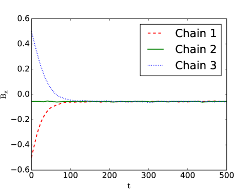
Starting from a point far from its value given by the minimization procedure is useful to check that this latter did not get stuck in a local minimum and that simulations starting from different points converge to the same region (see also section V.3). In practice, we have generated several chains (36 chains, to be more precise), starting from random points. We determined the thermalization time using equation (4) for each chain, and we removed from each chain its burn-in length.

V.2 Treatment of autocorrelations

By construction of a Markov chain, the state $\hat{q}_{t}$ depends strongly on the state $\hat{q}_{t-1}$ and quantities computed from this chain form themselves a Markov chain with inherent correlations from one member to the next. These type of correlations are often referred to as ”autocorrelations” in simulation time.

Let us consider that we would like to extract an observable $O$ from a Markov chain simulation with $N$ points. For this estimation, we use the $N$ successive Monte Carlo estimates $O_{t}$ (we assume in what follows, that the thermalization region has already been discarded, i.e. that the chain has been equilibrated before recording data) and we compute the usual mean $\langle O\rangle$ where $\langle.\rangle$ means averaging over the $N$ data points. The usual estimate of root-mean-square deviation of this average can be computed as

$$\sigma^{2}_{naive}=\frac{N}{N-1}\left(\langle O^{2}\rangle-\langle O\rangle^{2}\right)$$

This ”naive” error relies on the assumption that the measurements performed on the Markov chain are not correlated, which is in general not true. In order to account for the correlations, one can introduce for the given observable $O$, the integrated autocorrelation time $\tau_{int}$, which can be defined as follows:

$$\tau_{int}=\frac{1}{2}\displaystyle{\sum_{-\infty}^{+\infty}}\rho(s)$$

where $\rho(s)$ is the normalized autocorrelation function

$$\rho(s)=\frac{\left(O_{t}-\langle O\rangle\right)\left(O_{t+s}-\langle O\rangle\right)}{\left(O_{t}-\langle O\rangle\right)^{2}}$$

The dependence of $\rho(s)$ on the time separation $s$ only is a consequence of the chain being in equilibrium. The integrated autocorrelation time controls the statistical error in Monte Carlo measurement of $\langle O\rangle$ and there are mostly two possibilities to incorporate this autocorrelation time in the assessment of the statistical errors. The first one consists in leaving out $2\tau_{int}$ points between two effective points, or in other terms, to do a subsampling by rejecting all states which are closer than $2\tau_{int}$ to each other, in order to get independent states. This approach has the disadvantage of requiring the a priori knowledge of $\tau_{int}$. The second approach consists in keeping all measurements, but taking into account the autocorrelation time to estimate the statistical errors. The statistical error of correlated measurements can indeed by computed by Sokal_1989 ; Wolff_2003

$$\sigma^{2}_{\tau}=2\tau_{int}\sigma^{2}_{naive}$$

This means that the number of ”effectively independent data points” in a run of length $N$ is roughly $N/(2\tau_{int})$. If the integrated autocorrelation time is used to assess statistical errors, this means of course that a reliable estimate of $\tau_{int}$ and its error itself are needed. Such estimates require a delicate procedure. An efficient method – called $\Gamma$-method – has been developed in Wolff_2003 , which relies on the explicit determination of autocorrelation functions and autocorrelation times. This method provides not only numerical estimators of the integrated autocorrelation time, but also estimates for mean values and statistical errors for arbitrary functions of elementary observables in Monte Carlo simulations. We refer the interested reader to Wolff_2003 and references therein for details. We have used the $\Gamma$-method both to obtain the autocorrelation time and to compute observables.

A further method to reliably estimate the error on uncorrelated measurements is the so called Jackknife binning Quenouille_1956 . It consists in building $N$ subsets of data from the initial ensemble of size $N$, by removing one observation, leaving samples of size $N-1$. Pre-averaging over the blocks of data provides $N$ estimates of the average:

$$\langle O\rangle_{B}=\frac{1}{N-1}\left(\displaystyle{\sum_{t=1}^{(B-1)}}O_{t}+\displaystyle{\sum_{t=B+1}^{N}}O_{t}\right),\qquad B=1,\ldots,N$$

The jackknife mean and variance for the observable $O$ are then constructed from:

$${\langle O\rangle}_{Jack.}=\frac{1}{N}\displaystyle{\sum_{B=1}^{N}}\langle O\rangle_{B},\ \quad\sigma^{2}_{Jack.}=\frac{N-1}{N}\displaystyle{\sum_{B=1}^{N}}(\langle O\rangle_{B}-{\langle O\rangle}_{Jack.})^{2}$$

The jackknife method – and its extensions – is a widely used procedure, in particular in Lattice QCD. For cross-checks and comparison, we applied in our analysis both $\Gamma$-method and jackknife binning technics. For this latter, to un-correlate the points of a given chain, we performed a subsampling of this chain using the value of the autocorrelation time provided by the $\Gamma$-method.

V.3 Reversibility and convergence

We have verified that our implementation of HMC algorithm satisfies reversibility with a very good precision (relative accuracy better than $10^{-6}$) and that the average acceptance – computed using jackknife method, after removing thermalization region and decorrelating the chain – is $\langle e^{-\Delta H}\rangle=1.002\pm 0.016$, thus insuring that our chains indeed converge towards a stationary distribution. In addition, to exclude the risk of a non-identified lack of convergence, we have simulated several chains, with different (and random) starting points. This is illustrated in Figure 2 in the case of one varying parameter, namely $B_{g}$ (all others being fixed to their value obtained by standard $\chi^{2}$ minimization procedure), where the chains are clearly seen to converge towards the same stationary distribution.

Figure 2: Values of the parameter $B_{g}$ as a function of the Monte Carlo time for three independent Markov chains (l.h.s.). The starting points of the chains and the color code are the same as in Figure 1. The chains are clearly converging towards the same stationary distribution, what is confirmed by plotting the parameter distribution for each chain (r.h.s., after removing thermalization points and taking into account autocorrelation).

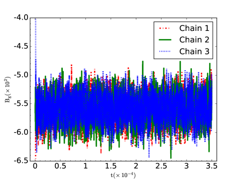
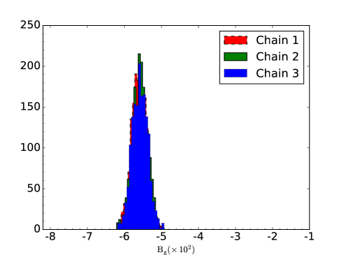
The results displayed in the next section have been obtained after skipping thermalization and properly taking into account the autocorrelation, using either the $\Gamma$-method or the Jackknife binning procedure as explained above.

VI Preliminary results

VI.1 Set-up and simulation parameters

The results shown in this section are obtained from a Markov Chain using the HERAPDF functional forms for initial PDFs at a scale $\mathrm{Q}_{0}=1.9$ GeV² with 10 free parameters: $B_{g}$, $C_{g}$, $B_{u_{val}}$, $C_{u_{val}}$, $E_{u_{val}}$, $C_{d_{val}}$, $C_{\overline{U}}$, $A_{\overline{D}}$, $B_{\overline{D}}$ and $C_{\overline{D}}$ (see expression (3) for the definition of these parameters, and HeraFitter for more details). We have used uniform priors for the parameters, and we consider the same data ensembles than the ones used to produce HERAPDF1.0 distributions.

These data are a combination of inclusive deep inelastic scattering cross-sections measured by the H1 and ZEUS Collaborations in neutral and charged current unpolarized $e^{\pm}p$ scattering at HERA, during the period 1994-2000 HeraFitter . Other settings and cuts – with the exception of the heavy flavor scheme, see below – were also identical to the ones of HERAPDF1.0 distributions. In particular, we do not rely of K factors, nor on grids techniques. The latter could however interestingly be used to speed up the computation.

Since the aim of this work is to demonstrate the applicability of MCMC methods to PDFs determination – rather than producing competitive PDF sets – we apply the ZMVFN scheme in order to speed up the computation of the $\chi^{2}$, and a lower cut on the data at $\mathrm{Q}_{min}^{2}=10$ GeV². These settings give a total number of data points of 537. We will denote by ”HERAPDF1.0 ZMVFNS” the PDFs thus obtained by minimization.

As already mentioned in the previous section, we have generated 36 Monte Carlo chains, each chain starting from a different random point, using the HMC algorithm.

The HMC algorithm requires the tuning of essentially two parameters: the number of leapfrog steps $L$ and the step size $\varepsilon$, this latter potentially depending on the direction in the parameter space. These two quantities are chosen such as to keep both the acceptance high (requiring small $\varepsilon$, to minimize the numerical errors in solving Hamilton equations), and the correlation between two successive Monte Carlo iterations small (thus requiring large trajectory length $L\varepsilon$). We have chosen $L=100$ and one leapfrog step size for each parameter, depending on the parameter typical standard deviation. Namely we took $\varepsilon_{i}=3.10^{-2}\Delta q^{typ}_{i}$, where $\Delta q^{typ}_{i}$ is, for each parameter, the value of its standard deviation provided by the minimization. With these HMC parameters, we obtain an acceptance of 80% and chains which have almost no correlation, since the integrated autocorrelation time $\tau_{int}$ computed by the $\Gamma$-method is less than 2 for all parameters.

The HMC algorithm also requires the computation of the potential energy (that is in our case the $\chi^{2}$) with respect to the parameters. These derivatives are computed numerically, using a symmetric derivative. We thus need, for 10 parameters, 20 evaluations of the $\chi^{2}$ for each step of the Leapfrog algorithm. We have run 36 jobs in parallel, and collected the results after three days of running. We computed for each of our 36 chains the burn-in length, and we removed the maximum burn-in (namely 28) to all of them, to obtain a total of 4 400 points per chain. To analyze these chains with the $\Gamma-$method, we kept all 158 400 points, while the jackknife analysis was done considering one point every four (i.e. $2\tau_{int}$), that is 39 600 points .

VI.2 PDFs parameter values, marginal distributions and correlations

Table 1 compares the mean value and its statistical error for each of the 10 PDFs parameters under consideration, using the two analysis procedures we have presented above, namely $\Gamma$-method and jackknife binning. The computation of the integrated autocorrelation time by the $\Gamma$-method gives values of $\tau_{int}$ less than 2 and we have used for the jackknife one point of the chain every four. As can be seen from Table 1, both methods give very close results, showing that we have analyze our Markov chain in a consistent way. For the rest of this paper, we will thus display only the results obtained using jackknife binning technics. We also notice that for the chain length considered ($\sim$ 40 000 thermalized and decorrelated points), the statistical errors on the mean values are tiny.

Table 1: Comparison of mean values and their statistical errors obtained for PDFs parameters using two different analysis methods. The jackknife binning has been applied after subsampling the chain, selecting points not closer than $2\tau_{int}=4$ from each other. Since the number of points considered for the jackknife analysis is thus four times less than for the $\Gamma-$method, the errors are expected to be smaller by roughly a factor 2 for this latter procedure, which is indeed the case.

parameter	$\Gamma$-method	jackknife binning
${\bf B}_{\bf g}$	$-0.0537\pm 0.0001$	$-0.0537\pm 0.0002$
${\bf C}_{\bf g}$	$5.9449\pm 0.0015$	$5.9483\pm 0.0025$
${\bf B}_{\mathrm{\bf u}_{\mathrm{\bf val}}}$	$0.6124\pm 0.0001$	$0.6125\pm 0.0002$
${\bf C}_{\mathrm{\bf u}_{\mathrm{\bf val}}}$	$4.7458\pm 0.0003$	$4.7455\pm 0.0006$
${\bf E}_{\mathrm{\bf u}_{\mathrm{\bf val}}}$	$14.965\pm 0.008$	$14.961\pm 0.012$
${\bf C}_{\mathrm{\bf d}_{\mathrm{\bf val}}}$	$3.2054\pm 0.0014$	$3.2077\pm 0.0016$
${\bf C}_{\overline{\bf U}}$	$4.0917\pm 0.0038$	$4.0961\pm 0.0048$
${\bf A}_{\overline{\bf D}}$	$0.3096\pm 0.0002$	$0.3098\pm 0.0002$
${\bf B}_{\overline{\bf D}}$	$-0.0174\pm 0.0001$	$-0.0173\pm 0.0002$
${\bf C}_{\overline{\bf D}}$	$6.2203\pm 0.0054$	$6.2096\pm 0.0076$

In Table 2 are displayed the results provided by MCMC method – using jackknife binning for error estimate – for the parameters mean, best fit and standard deviation, compared with the output of the standard MINUIT minimization.

Table 2: Comparison of results obtained for PDFs parameter values extracted from an independent Markov Chain of length 39 600, and the results provided from a MINUIT minimization. We compute from the MCMC the best fit value, the mean value and the standard deviation value for each of the 10 parameters considered, together with their statistical errors estimated by jackknife binning method. The standard deviation given by the minimization is the usual one-sigma deviation.

parameter	values	MCMC	MINUIT minimization
${\bf B}_{\bf g}$	mean	$\quad-0.0537\pm 0.0002\quad$
	best fit	$\quad-0.0632\pm 0.0168\quad$	$\qquad-0.0559\qquad$
	standard deviation	$\quad 0.0299\pm 0.0001\quad$	$\qquad 0.0288\qquad$
${\bf C}_{\bf g}$	mean	$\quad 5.9483\pm 0.0025\quad$
	best fit	$\quad 5.8952\pm 0.0615\quad$	$\qquad 5.9274\qquad$
	standard deviation	$\quad 0.5037\pm 0.0019\quad$	$\qquad 0.5078\qquad$
${\bf B}_{\mathrm{\bf u}_{\mathrm{\bf val}}}$	mean	$\quad 0.6125\pm 0.0002\quad$
	best fit	$\quad 0.6092\pm 0.0121\quad$	$\qquad 0.6098\qquad$
	standard deviation	$\quad 0.0371\pm 0.0001\quad$	$\qquad 0.0389\qquad$
${\bf C}_{\mathrm{\bf u}_{\mathrm{\bf val}}}$	mean	$\quad 4.7455\pm 0.0006\quad$
	best fit	$\quad 4.7467\pm 0.0525\quad$	$\qquad 4.7122\qquad$
	standard deviation	$\quad 0.1280\pm 0.0005\quad$	$\qquad 0.1332\qquad$
${\bf E}_{\mathrm{\bf u}_{\mathrm{\bf val}}}$	mean	$\quad 14.961\pm 0.012\quad$
	best fit	$\quad 15.42\pm 0.94\quad$	$\qquad 14.76\qquad$
	standard deviation	$\quad 2.494\pm 0.010\quad$	$\qquad 2.571\qquad$
${\bf C}_{\mathrm{\bf d}_{\mathrm{\bf val}}}$	mean	$\quad 3.2077\pm 0.0016\quad$
	best fit	$\quad 3.084\pm 0.076\quad$	$\qquad 3.143\qquad$
	standard deviation	$\quad 0.3183\pm 0.0016\quad$	$\qquad 0.2830\qquad$
${\bf C}_{\overline{\bf U}}$	mean	$\quad 4.0961\pm 0.0048\quad$
	best fit	$\quad 4.323\pm 0.814\quad$	$\qquad 4.052\qquad$
	standard deviation	$\quad 0.9617\pm 0.0035\quad$	$\qquad 0.9782\qquad$
${\bf A}_{\overline{\bf D}}$	mean	$\quad 0.3098\pm 0.0002\quad$
	best fit	$\quad 0.320\pm 0.039\quad$	$\qquad 0.305\qquad$
	standard deviation	$\quad 0.0485\pm 0.0002\quad$	$\qquad 0.0488\qquad$
${\bf B}_{\overline{\bf D}}$	mean	$\quad-0.0173\pm 0.0002\quad$
	best fit	$\quad-0.0097\pm 0.0237\quad$	$\qquad-0.0178\qquad$
	standard deviation	$\quad 0.0304\pm 0.0001\quad$	$\qquad 0.0306\qquad$
${\bf C}_{\overline{\bf D}}$	mean	$\quad 6.2096\pm 0.0076\quad$
	best fit	$\quad 5.888\pm 0.142\quad$	$\qquad 5.875\qquad$
	standard deviation	$\quad 1.505\pm 0.009\quad$	$\qquad 1.290\qquad$

We notice, as already stated above, that the determination of parameters by Monte Carlo methods, gives much more information than a minimization. We can in particular extract the statistical errors on the quantities we are interested in and this error decreases with the length of the Markov chain. As seen from the table, the most probable value extracted from the parameter probability distributions are compatible with the parameter values provided by the minimization procedure. For what concerns standard deviations however, although MCMC and minimization gives similar results, no precise comparison can be made since the minimization does not provide estimates of errors for the usual one-standard deviation of the parameters. In addition, both quantities (MCMC standard deviation and minimization deviation) should coincide only if the probability density of the parameter considered is Gaussian, which is not necessarily true (see below). This fact is already visible in Table 2, where we can see that the mean and best fit values do not coincide within errors for some of the parameters ($C_{d_{val}}$, $C_{\overline{D}}$ for instance).

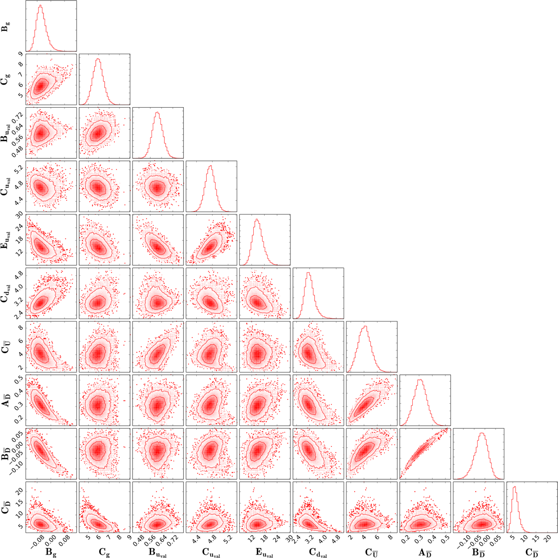
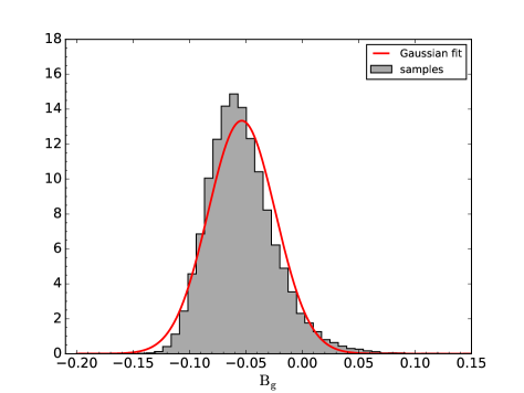
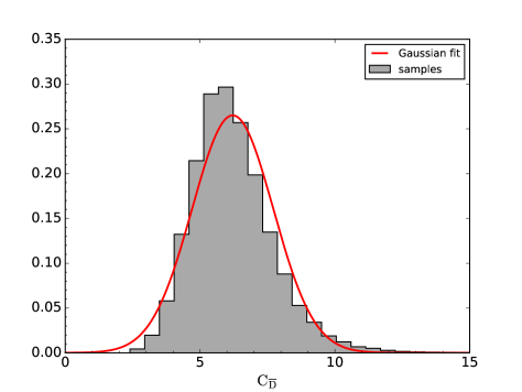
The probability distribution functions of the parameters, together with the 2D correlation plots between parameters are displayed in Figure 3. The marginal posterior parameter distributions are shown on the diagonal graphs, and 2D-correlations on the off-diagonal plots. The inner and outer contours of these latter are taken to be regions containing respectively 68% and 95% of the probability density. We note that the probability distribution of some parameters cannot properly be described by a Gaussian law, as illustrated in Figure 4, and are even non symmetric. We have also checked that our correlation plots are compatible with the values provided by the covariant matrix.

Figure 3: Probability distribution functions of the PDFs parameters (diagonal) and 2D correlation plots between parameters (off-diagonal).

Figure 4: Marginal probability distribution of parameters $B_{g}$ and $C_{\overline{D}}$. They do not follow a Gaussian law, as can be seen from the gaussian fit (solid red line).

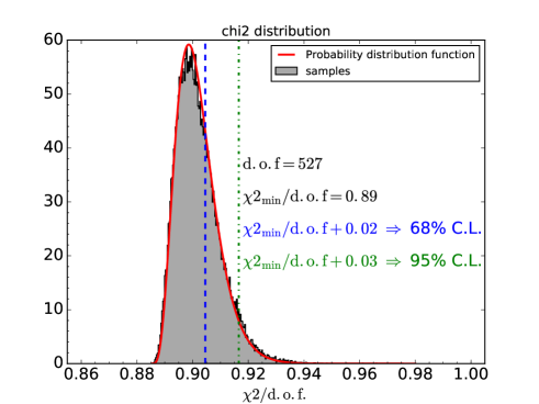
In Figure 5 is shown the $\chi^{2}/d.o.f.$ distribution for our 10-dimensional Monte Carlo chain. The solid red line is an adjustment with a $\chi^{2}$ distribution law with 10 degrees of freedom, which perfectly describes our results. The fact that the $\chi^{2}$ function built in equation (2) follows a $\chi^{2}$ distribution law with the expected number of degrees of freedom is a strong indication (though not a formal proof) that our assumptions concerning the fluctuations of the experimental data points around their corresponding theoretical values, are justified.

Figure 5: $\chi^{2}$ distribution for a 10D Monte Carlo chain. The solid red line is an adjustment of these data with a $\chi^{2}$ distribution law with 10 degrees of freedom. The dashed (dashdot) vertical line indicates the 68% (95%) confidence limit.

Though this is not the case in the example we present, we would also like to note that potential flat directions in the parameter space are less problematic for MCMC method than for minimization techniques.

We need now to calculate, from the Markov chain of parameters, the parton distribution functions we are interested in. The procedure we use is explained in the next section, and is more generally valid for any observable we want to compute from the MCMC.

VI.3 PDFs marginal distributions and confidence interval

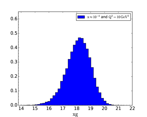
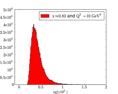
To extract parton distribution functions from the Markov chain, we compute, from the set of 10 parameters obtained at each Monte Carlo iteration, the corresponding PDFs for a range of $x$ and $Q^{2}$ values. This provides the marginal probability density functions of PDFs at fixed $(x,Q^{2})$, as illustrated on Figure 6 for the gluon, for two different $x$ values.

Figure 6: Gluon PDF probability distribution function for $x\approx 10^{-4}$ (l.h.s.) and $x\approx 0.83$ at fixed $Q^{2}=10$ GeV². The $68\%$ confidence interval is obtained from this distribution, considering the region of the distribution containing $68$% of the data remaining on each side of the best fit value.

For each $(x,Q^{2})$, we determine the $\alpha$%-confidence interval around the best fit value of the PDF (with typically $\alpha=68$ or $\alpha=95$) by considering the region of the distribution on each side of the best fit, and taking $\alpha$% of the data on each of these regions. This provides the (non necessarily symmetric) $\alpha$%-confidence limit envelops we show in Figures 7 to 11.

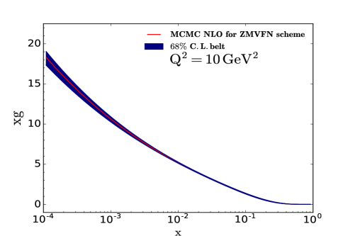
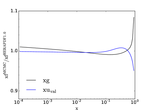
The gluon and $u_{val}$ parton distributions obtained this way are plotted as functions of $x$ and for $Q^{2}=10$ GeV² in Figure 7. The central PDF is the best fit value. These MCMC PDFs are compared with the HERAPDF1.0 PDFs (ZMVFN scheme), with a direct comparison in Figure 7, and a ratio plot in Figure 8. They are, as expected, very close, both in central value and in confidence interval. Maximum likelihood estimator and least square method are indeed equivalent under Gaussian assumption, which in our case can be reasonably applied, as mentioned in the previous section.

Figure 7: The parton distribution functions obtained using MCMC (right) compared to HERAPDF1.0 (ZMVFN scheme) from xFitter output (left) for $\mathrm{xu}_{\mathrm{val}}$ and $\mathrm{xg}$, at $\mathrm{Q^{2}}$ = $10\ \mathrm{GeV^{2}}$. The bands show the $68\%$ confidence interval around the central value (in solid red line) for the MCMC PDFs, and the standard $\Delta\chi^{2}=1$ deviation for HERAPDF.

Figure 8: Ratio of MCMC PDFs and HERAPDF1.0 (ZMVFN scheme) central values for $\mathrm{xu}_{\mathrm{val}}$ and $\mathrm{xg}$ at $\mathrm{Q^{2}}=10~{}\mathrm{GeV^{2}}$.

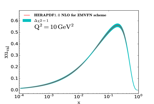
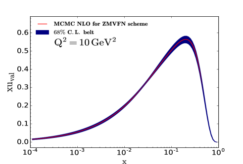
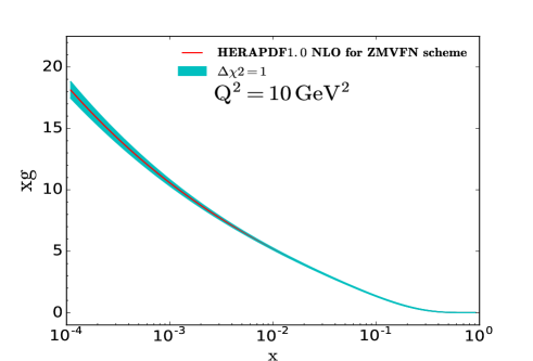
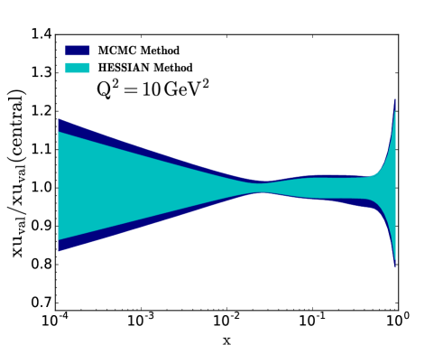
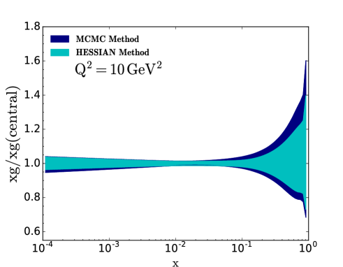
The uncertainties obtained by the MCMC method and the Hessian method are also consistent within the kinematic range of HERA. This is demonstrated in figure 9 where experimental uncertainties – normalized by the best fit value – obtained for HERAPDF1.0 NLO and MCMC NLO respectively by the Hessian and MCMC methods are compared for the $u_{val}$ and the gluon distributions. The MCMC uncertainties tend to be slightly larger than the standard deviations obtained in the Hessian approach.

Figure 9: Comparison of the PDF uncertainties, normalized by the best fit value, as determined by the Hessian and MCMC methods at NLO for the valence distribution $xu_{val}$ and the gluon distribution $xg$, at a scale $\mathrm{Q^{2}}$ = $10\ \mathrm{GeV^{2}}$.

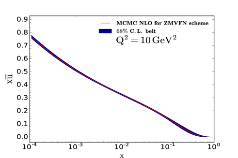
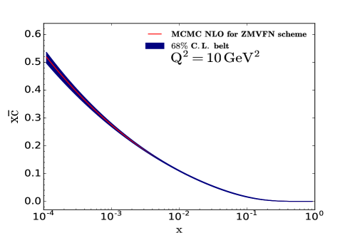
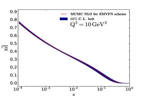
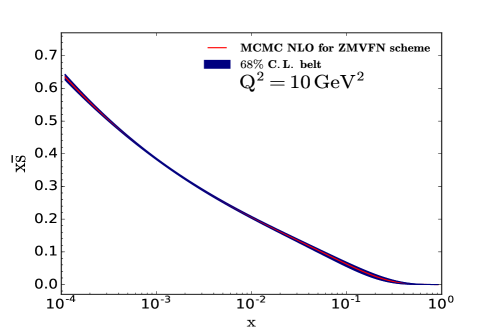
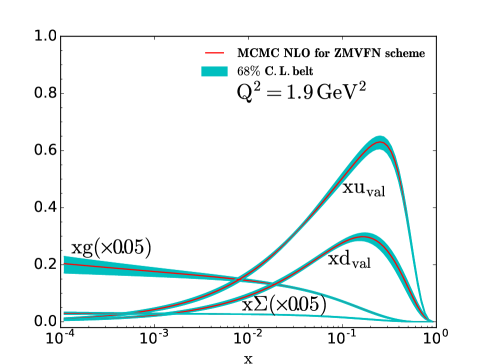
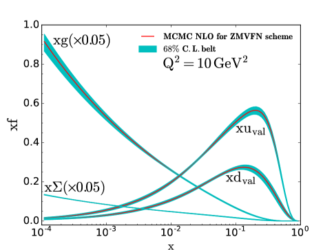
For completeness, we also display in Figure 10 the anti-quark PDFs at $Q^{2}=10$ GeV², and in Figure 11 the central value and 68% confidence limit interval for $xu_{val}$, $xd_{val}$, $xg$ and $x\Sigma$ ($x\Sigma=x\overline{u}+x\overline{d}+x\overline{s}+x\overline{c}$, with $x\overline{c}=0$ for $Q^{2}<m_{c}^{2}$) on the same plot, at $Q^{2}=1.9$ GeV² and $Q^{2}=10$ GeV².

Figure 10: The MCMC parton distribution functions $\mathrm{x\overline{u}}$, $\mathrm{x\overline{d}}$, $\mathrm{x\overline{s}}$ and $\mathrm{x\overline{c}}$ at $\mathrm{Q^{2}}$ = $10\ \mathrm{GeV^{2}}$. The bands show the $68\%$ confidence interval around the best fit value (in solid red line).

Figure 11: PDFs of valence quarks ($xu_{val}$, $xd_{val}$), sea quarks ($x\Sigma=x\overline{u}+x\overline{d}+x\overline{s}+x\overline{c}$, with $x\overline{c}=0$ for $Q^{2}<m_{c}^{2}$), and gluon ($xg$) using MCMC at the scale $\mathrm{Q^{2}}$ = $1.9\ \mathrm{GeV^{2}}$ (l.h.s.) and $\mathrm{Q^{2}}$ = $10\ \mathrm{GeV^{2}}$ (r.h.s.) obtained with the ZMVFN scheme. The gluon and the sea distributions are scaled down by a factor of 20. The experimental uncertainties (68% confidence limit as defined in the text from the probability density of PDFs) are represented by the green-shaded region.

VII Conclusion and outlook

We have shown that MCMC, known to be well suited to multi-parameter determination, is applicable to PDFs determination and that Bayesian parameter inference approach applied to global PDFs analysis can lead to a deeper insight into PDFs uncertainties. The innovative procedure we implemented, which combines Monte Carlo technics, lattice-developed algorithms and global PDFs analysis is complementary to the existing methods. We have for the first time applied Hybrid Monte Carlo algorithm to PDFs determination and computed marginal probability densities of PDFs parameters, and PDFs themselves. This allows to study the probability distribution of these functions, to determine mean, most probable and median values, and to extract confidence intervals in a statistically controlled way.

This work will lead to an innovative PDFs uncertainties determination, and thus to reliable determination of uncertainties for many collider observables, in a way complementary to the existing methods. This will also open new ways to analyze the impact of new data sets being added to the analysis, to check which dataset has outliers and if these latter can be tolerated.

This feasibility study paves the way for a more complete PDFs determination by MCMC technics, and our goal is to extend the present work to the full ensemble of PDFs free parameters, including also as parameters, the strong coupling constant and $c$ and $b$ quark masses. We will consider more complex $\chi^{2}$ functions including correlation and complete our analysis on a fully realistic case, studying in particular the impact of priors. No doubt that Markov Chain Monte Carlo methods will give interesting and valuable informations on PDFs and will contributed to our deeper understanding of these key elements of QCD.

VIII Acknowledgments

We thank L. Derome and D. Maurin for fruitful discussions, and the xFITTER support team for their help. We are also grateful to the CFM Foundation for Research for its financial support. Most of the computation has been done in Lyon-CCIN2P3, thanks to the CPUs resources provided. We are grateful to the staff members of this Computing Center for their constant support.

References

- (1) X. Ji, Phys.Rev.Lett. 110, 262002 (2013).
- (2) H. L. Lai, J. Huston, S. Kuhlmann, F. Olness, J. Owens, D. Soper, W. K. Tung, and H. Weerts, Phys. Rev. D55, 1280 (1997).
- (3) A. D. Martin, R. G. Roberts, M. G. Ryskin, W. J. Stirling, Eur. Phys. J. C2, 287 (1998); A. D. Martin, R. G. Roberts, W. J. Stirling and R. S. Thorne, Eur. Phys. J. C 28, 455 (2003); A.D. Martin, R.G. Roberts, W.J. Stirling, R.S. Thorne, Eur. Phys. J. C35, 325 (2004).
- (4) Walter T. Giele and Stephane Keller, Phys. Rev. D58, 094023 (1998).
- (5) J. Huston, E. Kovacs, S. Kuhlmann, H. L. Lai, J. F. Owens, D. Soper, and W. K. Tung, Phys. Rev. Lett. 77, 444 (1996).
- (6) J. Pumplin, D. Stump, R. Brock, D. Casey, J. Huston, J. Kalk, H.L. Lai, W.K. Tung, Phys. Rev. D65, 014013 (2001); J. Pumplin, D. R. Stump and W. K. Tung, Phys. Rev. D65, 014011 (2001); D. Stump, J. Pumplin, R. Brock, D. Casey, J. Huston, J. Kalk, H.L. Lai, W. K. Tung, Phys. Rev. D65, 014012 (2001);
- (7) D. Stump, J. Pumplin, R. Brock, D. Casey, J. Huston, J. Kalk, H.L. Lai, W.K. Tung, Phys. Rev. D65, 014012 (2001).
- (8) W. T. Giele and S. Keller, Phys. Rev. D58, 094023 (1998): W. T. Giele, S. Keller and D. Kosower, FERMILAB-PUB-01-498-T, arXiv:0104052 [hep-ph] (2001).
- (9) W.R. Gilks, S. Richardson and D.J. Speigelhalter, Markov Chain Monte Carlo in practice, Chapman & Hall/CRC Interdisciplinary Statistics ed., ISBN 9780412055515.
- (10) A. D. Sokal, Monte Carlo Methods in statistical machanics: foundations and new algorithms, Cours de Troisième Cycle de la Physique en Suisse Romande (Lausanne, Switzerland) (1989).
- (11) L. Del Debbio, S. Forte, J. I. Latorre, A. Piccione, and J. Rojo [NNPDF Collaboration], JHEP 0703, 039 (2007); J. C. Rojo, PhD thesis, hep-ph/0607122 (2006).
- (12) N. N. Nikolaev and B. Zakharov, Z. Phys. C49, 607 (1991); A. H. Mueller, Nucl. Phys. B 415, 373 (1994).
- (13) J. Collins, Foundations of perturbative QCD, vol. 32 (Cambridge monographs on particle physics, nuclear physics and cosmology, 2011).
- (14) S. M. Aybat and T. C. Rogers, Phys. Rev. D83, 114042 (2011); M. G. A. Buffing, A. Mukherjee, and P. J. Mulders, Phys. Rev. D86, 074030 (2012): P. Mulders, Pramana 72, 83 (2009) arXiv:0806.1134 [hep-ph]; S. Jadach and M. Skrzypek, Acta Phys. Polon. B40, 2071 (2009); F. Hautmann, Acta Phys. Polon. B40, 2139 (2009).
- (15) R. M. Neal in Handbook of Markov Chain Monte Carlo, S. Brooks, A. Gelman, G. L. Jones and X. Meng Ed., Chapman and Hall/CRC Press (2011).
- (16) N. Metropolis, A. W. Rosenbluth, M. N. Rosenbluth, A. H. Teller, and E. Teller, J. Chem Phys. 21, 1087 (1953).
- (17) W. K. Hastings, Biometrica, 57, 97 (1970).
- (18) M. de Berg, O. Cheong. M. van Kreveld and M. Overmars, Computational Geometry - Algorithms and Applications (Springer-Verlag), 2nd revised edition, ISBN: 978-3-662-04247-2.
- (19) S. Duane, A. D. Kennedy, B. J. Pendleton and D. Roweth, Phys. Lett. B195, 216 (1987).
- (20) A. Putze and L. Derome, Physics of the Dark Universe Vol. 5, 29 (2014).
- (21) A. Putze, L. Derome, D. Maurin, L. Perotto, and R. Taillet, Astron. Astrophys. Vol. 497 No 3, 991 (2009).
- (22) U. Wolff, Comput. Phys. Commun. 156, 143 (2004).
- (23) M. H. Quenouille, Biometrika, Vol. 43, No 3/4, 353 (1956).
- (24) S. Alekhin et al., Eur. Phys. J. C75 No 7, 304 (2015), http://www.xfitter.org/; H1 and ZEUS Collaboration (F.D. Aaron et al.), J.H.E.P. 1001, 109 (2010). H1 Collaboration (F.D. Aaron et al.), Eur. Phys. J. C64, 561 (2009); M. Botje, Comput. Phys. Commun. 182, 490 (2011); F. James, M. Roos (CERN), Comput. Phys. Commun. 10, 343 (1975); H1 Collaboration (C. Adloff et al.), Eur. Phys. J. C30,1 (2003); ZEUS Collaboration (S. Chekanov et al.), Phys. Rev. D67, 012007(2003); F.D. Aaron et al., Eur. Phys. J. C63, 625 (2009); ZEUS Collaboration (S. Chekanov et al.), Eur. Phys. J. C42, 1 (2005); J. Pumplin, D.R. Stump, J. Huston, H.L. Lai, P. M. Nadolsky, W.K. Tung, J.H.E.P. 0207, 012 (2002).