Non-Uniformly Coupled LDPC Codes: Better Thresholds, Smaller Rate-loss, and Less Complexity

Abstract

We consider spatially coupled low-density parity-check codes with finite smoothing parameters. A finite smoothing parameter is important for designing practical codes that are decoded using low-complexity windowed decoders. By optimizing the amount of coupling between spatial positions, we show that we can construct codes with excellent thresholds and small rate loss, even with the lowest possible smoothing parameter and large variable node degrees, which are required for low error floors. We also establish that the decoding convergence speed is faster with non-uniformly coupled codes, which we verify by density evolution of windowed decoding with a finite number of iterations. We also show that by only slightly increasing the smoothing parameter, practical codes with potentially low error floors and thresholds close to capacity can be constructed. Finally, we give some indications on protograph designs.

I Introduction

Low-density parity-check (LDPC) codes are widely used due to their outstanding performance under low-complexity belief propagation (BP) decoding. However, an error probability exceeding that of maximum-a-posteriori (MAP) decoding has to be tolerated with (sub-optimal) low-complexity BP decoding. A few years ago, it has been empirically observed that the BP performance of some protograph-based, spatially coupled (SC) LDPC ensembles (also termed convolutional LDPC codes) can improve towards the MAP performance of the underlying LDPC ensemble [1]. Around the same time, this threshold saturation phenomenon has been proven rigorously in [2, 3] for a newly introduced, randomly coupled SC-LDPC ensemble. In particular, the BP threshold of that SC-LDPC ensemble tends towards its MAP threshold on any binary memoryless symmetric channel (BMS).

SC-LDPC ensembles are characterized by two parameters: the replication factor $L$, which denotes the number of copies of LDPC codes to be places along a spatial dimension, and the smoothing parameter $w$. This latter parameter indicates that each edge of the graph is allowed to connect to $w$ neighboring spatial positions (for details, see [2] and Sec. II). The proof of threshold saturation was given in the context of uniform spatial coupling and requires both $L\to\infty$ and $w\to\infty$. This poses a serious disadvantage for realizing practical codes, as relatively large structures are required to build efficient codes.

In practice, the main challenges for implementing SC-LDPC codes are the rate-loss due to termination and the decoding complexity. The rate-loss, which scales with $w$, can be made arbitrarily small by increasing $L$, however, a large $L$ can worsen the finite-length performance of SC-LDPC codes [4]. Known approaches to mitigate the rate-loss (e.g., [5, 6]) often introduce extra structure at the boundaries, which is usually undesired. Therefore, we would like to keep the rate-loss as small as possible for a fixed, but small $L$. Additionally, the decoding complexity can be managed by employing windowed decoding (WD) [7], however, the window length and complexity scale with the smoothing parameter $w$. For both reasons, $w$ should be as small as possible, ideally $w\in\{2,3\}$, to keep the rate-loss and complexity small, e.g., in high-speed optical communications [8].

In this paper, we construct code ensembles that have excellent thresholds for small $w$, that have smaller rate-loss than SC-LDPC ensembles and can be decoded with less complexity by maximizing the speed of the decoding wave. We achieve these properties by generalizing the uniformly coupled SC-LDPC codes of [2] to allow for non-uniform coupling. It was already recognized in [9, 10] that non-uniform protographs can lead to improved thresholds in some circumstances by sacrificing a one-sided converge of the chain, which is not problematic when using WD. A very particular, exponential coupling was used in [11] to guarantee anytime reliability.

We extend non-uniform coupling to randomly coupled SC-LDPC ensembles and protograph-based ensembles. We analyze their performance under message passing with and without windowed decoding. We show that we can achieve excellent close-to-capacity thresholds by optimizing the coupling, for small $w$ and large $d_{v}$, which is required for codes with low error floors. Furthermore, we introduce a new multi-type-based non-uniform coupling that further improves the thresholds without increasing $w$. We find that the rate-loss is decreased by non-uniform coupling as well. We finally show that the decoding speed, which is an indicator of the complexity, can be increased by non-uniform coupling.

II Spatially Coupled LDPC Codes

We briefly describe two construction types of non-uniformly coupled LDPC codes: the random ensemble and the protograph-based ensemble. The former is easier to analyze and exhibits the general advantages of non-uniform coupling while the latter is more of practical interest.

II-A The Random $(d_{v},d_{c},\bm{\nu},L,M)$ Ensemble

We now briefly review how to sample a code from a random, non-uniformly coupled ($d_{v},d_{c},\bm{\nu},L,M$) SC-LDPC ensemble with regular degree distributions. We first lay out a set of positions indexed from $z=1$ to $L$ on a spatial dimension. At each spatial position (SP) $z$, there are $M$ variable nodes (VNs) and $M\frac{d_{v}}{d_{c}}$ check nodes (CNs), where $M\frac{d_{v}}{d_{c}}\in\mathbb{N}$ and $d_{v}$ and $d_{c}$ denote the variable and check node degrees, respectively. The non-uniformly coupled structure is based on the smoothing distribution $\bm{\nu}=[\nu_{0},\dots,\nu_{w-1}]$ where $\nu_{i}>0$, $\sum_{i}\nu_{i}=1$ and $w>1$ denotes the smoothing (coupling) width. The special case of $\nu_{i}=\frac{1}{w}$ leads to the usual, well-known spatial coupling with the uniform smoothing distribution [3].

For termination, we additionally consider $w-1$ sets of $M\frac{d_{v}}{d_{c}}$ CNs in SPs $L+1,\dots,L+w-1$. Every CN is assigned with $d_{c}$ “sockets” and imposes an even parity constraint on its $d_{c}$ neighboring VNs. Each VN in SP $z$ is connected to $d_{v}$ CNs in SPs $z,\ldots,z+w-1$ as follows: For each of the $d_{v}$ edges of this VN, an SP $z^{\prime}\in\{z,\ldots,z+w-1\}$ is randomly selected according to the distribution $\bm{\nu}$, and then, the edge is uniformly connected to any free socket of the $Md_{v}$ sockets arising from the CNs in that SP $z^{\prime}$. This graph represents the code with $n=LM$ code bits, distributed over $L$ SPs. Because of additional CNs in SPs $L+1,\ldots,L+w-1$, but also because of potentially unconnected CNs in SPs $1,\ldots,w-1$, the design rate is slightly decreased to $r=1-\frac{d_{v}}{d_{c}}-\frac{1}{L}\Delta$ where

$$\Delta=\frac{d_{v}}{d_{c}}\left(w\!-\!1\!-\!\sum_{k=0}^{w-2}\left[\left(\sum_{i=0}^{k}\nu_{i}\right)^{d_{c}}\!\!\!+\left(\sum_{i=k+1}^{w-1}\nu_{i}\right)^{d_{c}}\right]\right)$$

which increases linearly with $w$.

In the limit of $M$, the asymptotic performance of this ensemble on a binary erasure channel (BEC) can be analyzed using density evolution, with

$$x_{z}^{(t+1)}=\varepsilon\!\left(\!1\!-\!\sum_{i=0}^{w-1}\nu_{i}\left(1\!-\!\sum_{j=0}^{w-1}\nu_{j}x_{z+i-j}^{(t)}\right)^{d_{c}-1}\right)^{d_{v}-1}$$ (1)

where $\varepsilon$ denotes the channel erasure probability and $x_{z}^{(t)}$ the average erasure probability of the outgoing messages from VNs in SP $z$ at iteration $t$. The messages are initialized as $x_{z}^{(0)}=\varepsilon$, if $z\in[1,L]$ and $x_{z}^{(0)}=0$ otherwise. For $\nu_{i}=\frac{1}{w}$, (1) becomes the known DE equation for SC-LDPC codes with uniform coupling [2, Eq. (7)].

II-B Protograph-based SC-LDPC Ensembles

SC-LDPC ensembles with a certain predefined structure can be constructed by means of protographs [12]. The Tanner graph of the protograph-based SC-LDPC code is some $M$-cover of the protograph, i.e., $M$ copies of the protograph are bound together by random permutation of the edges between the same type of sockets. Protograph-based SC-LDPC codes are of practical interest because of their simple hardware implementation and their excellent finite-length performance [13]. An exemplary protograph of an SC-LDPC code with non-uniform coupling is shown in Fig. 1-a). As the coupled protograph is a chain of repeating segments, we represent coupled protographs by their distinct elementary segment shown in Fig. 1-b). We use the 3-tuple $(d_{v},b_{1},b_{2})$ to describe the elementary segment, with $d_{v}$ the regular variable node degree, $b_{1}$ the number of parallel edges between VN $v_{1}$ and CN $c_{1}$ and $b_{2}$ the number of parallel edges between VN $v_{2}$ and CN $c_{1}$.

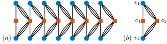
Figure 1: Protograph of a $(d_{v}=4,d_{c}=8,L=7,w=2)$ SC-LDPC ensemble with non-uniform coupling $(b)$ The elementary segment of the chain denoted by the 3-tuple $(4,1,1)$.

II-C Windowed Decoder Complexity

The decoding complexity is an important parameter for practical SC-LDPC codes. Consider the profile of densities $[x_{0}^{(t)},x_{1}^{(t)},\dots]$ in (1). It has been shown in [2, 14] that the profile behaves like a “wave”: it shifts along the spatial dimension with “a constant speed” as the BP decoder iterates. The wave propagation speed is analytically analyzed and bounded in [15],[16].

The wave-like behaviour enables efficient sliding windowed decoding [7]: the decoder updates the BP messages of edges lying in a window of $W_{D}$ SPs $I$ times, and then shifts the window one SP forward and repeats. Thus, the decoding complexity scales with $O(W_{D}ILMd_{v})$ as there are $2MLd_{v}$ BP messages and each BP message is updated $W_{D}I$ times.

The required window size $W_{D}$ is an increasing function of the smoothing factor $w$ [7] which implies that we should keep $w$ small. The number of iterations $I>\frac{1}{v}$ where $v$ is the speed of the wave. In the continuum limit of the spatial dimension, $v$ is defined as the amount displacement of the profile along the spatial dimension after one iteration. For the discrete case of (1), the speed can be estimated by

$$v\approx v_{D}=\frac{D}{T_{D}},$$ (2)

where $T_{D}$ in the minimum number of iterations required for the displacement of the profile by more than $D$ SPs, i.e.,

$$T_{D}=\min\{T\in\mathbb{N}\mid x_{z}^{(t+T)}\leq x_{z-D}^{(t)},\;{\rm for}\;t>0\;\wedge\;z\leq\lfloor L/2\rfloor\}.$$

The approximation of $v$ becomes more precise by choosing larger $D$. We chose $D=10$ in this paper.

We quickly recapitulate the asymptotic analysis for the windowed decoder here. Instead of the windowed decoder proposed in [7, Def. 4], we employ a slightly modified, more practical version, which updates the complete window after one decoding step. For every windowed decoding step, indexed by $c\in[1,L]$, we generate a copy $\bm{y}_{c,z}^{(0)}$ of the vector $\bm{x}=(x_{1}^{(c-1)},\ldots,x_{L+w-1}^{(c-1)})$ on which we apply the update rule (1) for SPs $z\in\{c,c+1,\ldots,c+W_{D}-1\}$ only, for a total of $I$ iterations. After $I$ iterations, we update the SPs as

$$x_{z}^{(c)}=\left\{\begin{array}[]{ll}x_{z}^{(c-1)}&\text{if }z\not\in[c,c+W_{D})\\ y_{z-c+1}^{(I)}&\text{otherwise}\end{array}\right.$$

We use a finite number of iterations in the windowed decoder to accurately predict the performance of a practical decoder.

III Non-Uniform Coupling: Random Ensembles

In this section, we optimize non-uniformly SC-LDPC ensembles with random coupling for the BEC. First, we consider $w=2$, the smallest possible smoothing parameter. This case has a high practical interest as $w$ should be kept as small as possible in order to keep the decoding latency and window length $W_{D}$ manageable when employing windowed decoding. We show numerically that non-uniform coupling improves the BP threshold and also the decoding complexity as the total number of iterations decreases. Afterwards, we show the advantages of non-uniform coupling $w>2$.

III-A Non-Uniform Unit-Memory Coupling ($w=2$)

Consider a random $(d_{v},d_{c},\bm{\nu},L,M)$ SC-LDPC ensemble with smoothing vector $\bm{\nu}=[\alpha,1-\alpha]$. It is enough to assume $0\leq\alpha\leq\frac{1}{2}$ because of symmetry. In the limit of $M$, the asymptotic performance of the ensemble over BEC can be evaluated using DE. We consider the BP threshold

$$\varepsilon_{\rm\scriptscriptstyle BP}(\alpha)=\sup\{\varepsilon:x_{z}^{(\ell)}\to 0\text{ as }\ell\to\infty,\forall z\in[1,L]\},$$

where $x_{z}^{(\ell)}$ is updated according to (1). Figure 2 illustrates $\varepsilon_{\rm\scriptscriptstyle BP}(\alpha)$ in terms of $\alpha$ for different values of $d_{v}$.

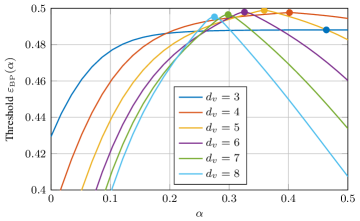
Figure 2: Thresholds for the $(d_{v},2d_{v},[\alpha,1-\alpha],L=100)$ ensemble (with $w=2$ and rate $\approx\frac{1}{2}(1-\frac{1}{L})$).

Each curve has two minima and a maximum. The two minima are at $\alpha=0$ and $\alpha=\frac{1}{2}$ where $\varepsilon_{\rm\scriptscriptstyle BP}(\alpha=0)=\varepsilon_{\rm\scriptscriptstyle BP,uncoupl.}$ corresponds to the BP threshold of the uncoupled ensemble and $\varepsilon_{\rm\scriptscriptstyle BP}(\alpha=\frac{1}{2})$ corresponds to the BP threshold of the SC-LDPC ensemble with uniform coupling. The respective maxima of the curves are indicated by a marker and obtained for $\alpha^{*}$. We can see that uniform coupling ($\alpha=1/2$) does not lead to the best thresholds. In particular, if we increase $d_{v}$, which is required for constructing codes with very low error floors, uniform coupling with $w=2$ is not efficient anymore, and the thresholds are significantly away from the BEC capacity. With an optimized $\alpha^{\star}$, we can achieve thresholds that are close to capacity (and the MAP threshold of the uncoupled LDPC ensemble $\varepsilon_{\rm\scriptscriptstyle MAP,uncoupl.}$) and significantly outperform the uncoupled and the uniformly coupled cases. Table I gives the thresholds of the optimized codes together with the unoptimized, uniformly coupled and uncoupled cases. Although coupling always improves the threshold, with $w=2$, uniform coupling is not a good solution and significantly better thresholds are obtained by non-uniform coupling, especially for larger $d_{v}$. Moreover, it is easy to show that the rate-loss $\Delta$ is maximized for uniform coupling ($\alpha=1/2$). Hence non-uniform coupling will always reduce the rate-loss. We can see that as $d_{v}$ increases, $\alpha^{\star}$ decreases as well. An interesting open question is whether $\alpha$ saturates to some constant or if it will converge to zero.

TABLE I: Optimal $\alpha^{\star}$ and the BP and MAP thresholds of the uncoupled codes, $\varepsilon_{\rm\scriptscriptstyle BP,uncoupl.}$ and $\varepsilon_{\rm\scriptscriptstyle MAP,uncoupl.}$, and BP thresholds of the uniformly coupled codes, $\varepsilon_{\rm\scriptscriptstyle BP}(\alpha=1/2)$, and with optimized $\alpha^{\star}$ for different rate $\approx\frac{1}{2}(1-\frac{1}{L})$ with regular VN degree $d_{v}$.

$d_{v}$	$\alpha^{\star}$	$\varepsilon_{\rm\scriptscriptstyle BP,uncoupl.}$	$\varepsilon_{\rm\scriptscriptstyle MAP,uncoupl.}$	$\varepsilon_{\rm\scriptscriptstyle BP}(\alpha=1/2)$	$\varepsilon_{\rm\scriptscriptstyle BP}(\alpha^{\star})$
3	0.4517	0.4294	0.48815	0.4880(8)	0.4881(0)
4	0.4017	0.3834	0.49774	0.4944	0.4976
5	0.3590	0.3415	0.49949	0.4827	0.4989
6	0.3252	0.3075	0.49988	0.4603	0.4979
7	0.2978	0.2798	0.49997	0.4338	0.4965
8	0.2745	0.2570	0.49999	0.4074	0.4953
9	0.2544	0.2378	0.49999	0.3829	0.4943
10	0.2368	0.2215	0.49999	0.3606	0.4936

Non-uniform coupling can also decrease the decoding complexity of windowed decoding. Figure 3 illustrates the effect of non-uniform coupling on the wave propagation. While uniform coupling ($\alpha=\frac{1}{2}$) leads to a wave propagation from both ends towards the middle, non-uniform coupling sacrifices one of those waves in favor of the other one, which will (usually) travel at a faster velocity.

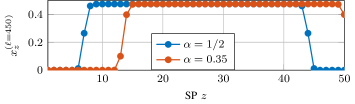
Figure 3: Average message erasure probability $x_{z}^{(\ell)}$ for the $(5,10,\alpha,50)_{w=2}$ ensemble for $\alpha\in\{0.35,1/2\}$ and with $\ell=450$ for $\epsilon=0.48$.

We compute the speed $v$ according to (2) for different values of $\alpha\in[0,1/2]$ and different values of $\varepsilon\in[\varepsilon_{\rm\scriptscriptstyle BP}(\alpha=0),\varepsilon_{\rm\scriptscriptstyle BP}(\alpha^{\star})]$ and show the contour lines of equal decoding speed $v$ in Fig. 4 for $d_{v}=5$ and $d_{v}=10$. Points along a contour line indicate that the decoding wave moves with the same speed. When building practical decoders, usually a hardware constraint is imposed which limits the amount of operations that can be done. Hence also the decoding speed is limited. We can see that for a fixed speed $v$, non-uniformly coupled codes can be operated at much higher erasure probability than with uniform coupling. Note that the maxima of the speed contours coincide practically with the $\alpha^{\star}$ maximizing the threshold.

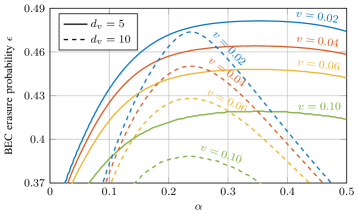
Figure 4: Decoding speed contour lines for the random $(5,10,[\alpha,1-\alpha],L=100)$ SC-LDPC ensemble (solid curves) and the $(10,20,[\alpha,1-\alpha],L=100)$ SC-LDPC ensemble (dashed curves) with design rate $\approx\frac{1}{2}(1-\frac{1}{L})$.

Figure 4 suggests that windowed decoding also benefits from non-uniform coupling. For this reason, we use density evolution including windowed decoding, as detailed in Sec. II-C. Figure 5 exemplarily shows the thresholds for windowed decoding for the $(5,10,[\alpha,1-\alpha],L=100)$ and the $(10,20,[\alpha,1-\alpha],L=100)$ SC-LDPC ensembles for four window configurations: $W_{D}\in\{10,20\}$ and $I\in\{3,9\}$. We see a good agreement between the speed contour lines of Fig. 4 and the windowed decoding thresholds. Again we can see that for non-uniformly coupled codes and identical window configurations, we can significantly increase the decoding threshold.

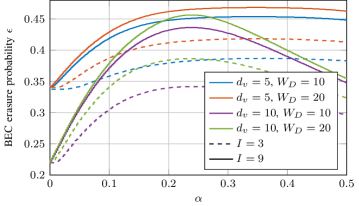
Figure 5: Windowed decoding thresholds for the $(5,10,[\alpha,1-\alpha],L=100)$ and $(10,20,[\alpha,1-\alpha],L=100)$ ensembles for different window configurations as a function of $\alpha$.

III-B Non-Uniform Coupling with $w>2$

We have seen in the previous section that non-uniform coupling can increase the BP threshold if we constrain $w=2$. However, for $d_{v}>5$, we have to tolerate a gap to capacity. In this case, we can relax the constraint on $w$. In fact, for $w>2$, non-uniform coupling can be more beneficial as there are more degrees of freedom for optimizing the smoothing vector $\bm{\nu}$. We numerically show in the following that it results in a faster saturation of the BP threshold to capacity even for small values of $w$, e.g., $w=3$.

Consider the DE equation (1) for a random $(d_{v},d_{c},\bm{\nu},L)$ SC-LDPC ensemble over a BEC. Let $\bm{\nu}=[\nu_{1},\nu_{2},1-\nu_{1}-\nu_{2}]$ with $w=\text{dim}(\bm{\nu})=3$. For regular ensembles with asymptotic rate $r=\frac{1}{2}$ ($d_{c}=2d_{v}$), we observe that the BP threshold, $\varepsilon_{\rm\scriptscriptstyle BP}(\bm{\nu})$, depends on the choice of $\bm{\nu}$ and can get very close to the capacity. We used a grid search with a fine resolution to numerically optimize the BP threshold for the ensembles with $d_{v}\in\{4,\ldots,10\}$. The results are given in Tab. II where the optimized smoothing distribution is denoted by $\bm{\nu}^{\star}=[\nu_{1}^{\star},\nu_{2}^{\star},1-\nu_{1}^{\star}-\nu_{2}^{\star}]$. We observe that the BP thresholds almost saturate to the capacity (or $\varepsilon_{\rm\scriptscriptstyle MAP,uncoupl.}$, respectively), while the BP threshold of uniformly coupled ensembles ($\varepsilon_{\rm\scriptscriptstyle BP}(\bm{\nu}=[\frac{1}{3},\frac{1}{3},\frac{1}{3}])$) have a gap to capacity which increases for larger $d_{v}$. Note that especially for small $d_{v}$, many different choices of $\bm{\nu}$ lead to good thresholds $\varepsilon_{\rm\scriptscriptstyle BP}$. In that case, we select the optimum $\bm{\nu}^{\star}$ which leads to a good threshold and also yields a small rate loss $\Delta$. Note that in contrast to the $w=2$ case, where the rate-loss was maximal for uniform coupling, it is not hard to show that the rate-loss $\Delta$ for $w=3$ is maximized with $\bm{\nu}=[\frac{1}{2},0,\frac{1}{2}]$. It is an interesting open question whether it is possible to construct capacity-achieving codes with a finite $w$.

TABLE II: Optimal $\bm{\nu}$ and the BP thresholds of the uniformly coupled codes $\varepsilon_{\rm\scriptscriptstyle BP}(\bm{\nu}=[\frac{1}{3},\frac{1}{3},\frac{1}{3}])$ and with optimized $\bm{\nu}^{\star}=[\nu_{1}^{\star},\nu_{2}^{\star},1-\nu_{1}^{\star}-\nu_{2}^{\star}]$ for the random $(d_{v},2d_{v},\bm{\nu},L=100)$ SC-LDPC ensembles with rate $\approx\frac{1}{2}(1-\frac{2}{L})$, as well as rate-losses $\Delta$ for both uniform and non-uniform coupling.

$d_{v}$	$\nu_{1}^{\star}$	$\nu_{2}^{\star}$	$\varepsilon_{\rm\scriptscriptstyle BP}([\frac{1}{3},\frac{1}{3},\frac{1}{3}])$	$\varepsilon_{\rm\scriptscriptstyle BP}(\bm{\nu}^{\star})$	$\Delta([\frac{1}{3},\frac{1}{3},\frac{1}{3}])$	$\Delta(\bm{\nu}^{\star})$
3	0.0789	0.4737	0.48815	0.4881(5)	0.911	0.676
4	0.1842	0.4211	0.4977	0.4977(4)	0.961	0.893
5	0.2632	0.2105	0.4989	0.4994(7)	0.983	0.975
6	0.2465	0.1496	0.4967	0.4998(7)	0.992	0.982
7	0.2355	0.1247	0.4904	0.4999(7)	0.997	0.987
8	0.2244	0.1025	0.4797	0.4999(8)	0.998	0.991
9	0.2147	0.0803	0.4652	0.4999(5)	0.999	0.993
10	0.2063	0.0665	0.4486	0.4999(4)	1.000	0.994

III-C Non-Uniform Coupling with Different Types

Non-uniform coupling is a general concept. So far, we presented the simplest way of non-uniform coupling in which the edges of all VNs in an SP are randomly connected according to a distribution $\bm{\nu}$. Generally, the edges of each VN can be connected according to a set of distributions. Let us illustrate the benefits of such coupling by an example. Consider again a coupled LDPC ensemble with $w=2$ and $d_{c}=2d_{v}$. Inspired by the protograph structure shown in Fig. 1, we partition the VNs in each SP into two sets of equal size, called “upper set” and “lower set”. As described in Sec. II-A, the edges of VNs in the upper set are randomly connected to CNs according to the “upper” smoothing distribution $\overline{\bm{\nu}}=[\overline{\alpha},1-\overline{\alpha}]$. Similarly, the edges of VNs in the lower set are distributed according to the “lower” smoothing distribution $\underline{\bm{\nu}}=[\underline{\alpha},1-\underline{\alpha}]$. Therefore, each CN receives two types of BP messages from VNs. Let $\overline{x}_{z}^{(t)}$ ($\underline{x}_{z}^{(t)}$) denote the average erasure probability of the BP messages flowing from VNs of the upper set (lower set) in SP $z$ at iteration $t$. Then the DE equations become

$$\overline{y}_{z}^{(t)}\!=\!\left(1\!-\!(\overline{\alpha}\overline{x}_{z}^{(t)}\!+\!(1\!-\!\overline{\alpha})\overline{x}_{z-1}^{(t)})\right)^{d_{v}\!-\!1}\!\!\left(1\!-\!(\underline{\alpha}\underline{x}_{z}^{(t)}\!+\!(1\!-\!\underline{\alpha})\underline{x}_{z-1}^{(t)})\right)^{d_{v}}$$

$$\underline{y}_{z}^{(t)}\!=\!\left(1\!-\!(\overline{\alpha}\overline{x}_{z}^{(t)}\!+\!(1\!-\!\overline{\alpha})\overline{x}_{z-1}^{(t)})\right)^{d_{v}}\!\!\left(1\!-\!(\underline{\alpha}\underline{x}_{z}^{(t)}\!+\!(1\!-\!\underline{\alpha})\underline{x}_{z-1}^{(t)})\right)^{d_{v}\!-\!1}$$

$$\overline{x}_{z}^{(t+1)}=\varepsilon\left(1-(\overline{\alpha}\overline{y}_{z}^{(t)}+(1-\overline{\alpha})\overline{y}_{z+1}^{(t)})\right)^{d_{v}-1}$$

$$\underline{x}_{z}^{(t+1)}=\varepsilon\left(1-(\underline{\alpha}\underline{y}_{z}^{(t)}+(1-\underline{\alpha})\underline{y}_{z+1}^{(t)})\right)^{d_{v}-1}$$

Using DE analysis and a rough exhaustive search, we optimized $\overline{\alpha}$ and $\underline{\alpha}$ to find the largest BP threshold for different values of $d_{v}$. The thresholds are summarized in Tab. III. We observe that the thresholds almost saturate to capacity for $d_{v}=6$ and $d_{v}=7$ with only $w=2$.

TABLE III: Non-uniform coupling with two types: BP thresholds of random non-uniformly coupled ensembles with $d_{c}=d_{v}$, $w=2$, $L=100$ and optimal $[\overline{\alpha}^{\star},1-\overline{\alpha}^{\star}]$ and $[\underline{\alpha}^{\star},1-\underline{\alpha}^{\star}]$.

$d_{v}$ $\overline{\alpha}^{\star}$ $\underline{\alpha}^{\star}$ $\varepsilon_{\rm\scriptscriptstyle BP}$ 5 0.350 0.362 0.4989 6 0.278 0.375 0.4998 7 0.248 0.349 0.4998

$d_{v}$ $\overline{\alpha}^{\star}$ $\underline{\alpha}^{\star}$ $\varepsilon_{\rm\scriptscriptstyle BP}$ 8 0.227 0.323 0.4996 9 0.209 0.300 0.4995 10 0.195 0.279 0.4994

IV Non-Uniform Coupling: Protograph Ensembles

As most practical codes are based on protographs, we extend the findings of this paper to protograph-based codes with the elementary building segment of Fig. 1-b). In comparison to the random ensembles, there is less room for optimization as there are finite choices for $b_{1}$ and $b_{2}$, each requiring a separate DE analysis, which is also slightly more complicated as the BP messages come from different edge types (multi-edge types DE). We computed DE thresholds for all possible protographs based on a simple elementary segment with 2 VNs and 2 CNs for $L=100$ ($r=0.495$). In Tab. IV, we summarize the best protographs and the respective thresholds that we find for different choices of $d_{v}$. Some of the best elementary segments are shown in Fig. 6. Up to $d_{v}=6$, protographs with $b_{1}=b_{2}=1$ are optimal, however, when $d_{v}>6$, interestingly, the choice $b_{1}=1$ and $b_{2}=5$ becomes optimal.

TABLE IV: Thresholds of non-uniformly coupled regular protograph ensembles with simple elementary protographs.

$(d_{v},b_{1},b_{2})$ Threshold $\varepsilon_{\rm BP}$ $(3,1,1)$ 0.48815 $(4,1,1)$ 0.49741 $(5,1,1)$ 0.49811 $(6,1,1)$ 0.49667 $(7,1,5)$ 0.49257 $(8,1,5)$ 0.49451 $(9,1,5)$ 0.49627 $(10,1,5)$ 0.49711

$(d_{v},b_{1},b_{2})$ Threshold $\varepsilon_{\rm BP}$ $(11,1,5)$ 0.49693 $(12,1,5)$ 0.49612 $(13,1,5)$ 0.49502 $(14,1,5)$ 0.49377 $(15,1,5)$ 0.49246 $(16,1,5)$ 0.49113 $(17,1,5)$ 0.48981 $(18,1,5)$ 0.48850

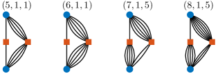
Figure 6: Example of optimized protographs, represented by their elementary segment, with various unequal coupling for $d_{v}\in\{5,6,7,8\}$.

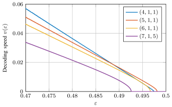
Figure 7: Decoding speeds for different optimal protographs.

In Fig. 7, we plot the decoding speeds for the best protographs with $d_{v}\in\{4,5,6,7\}$. We can see that for $\varepsilon<0.488$, the protograph $(4,1,1)$ has the highest decoding speed and thus leads to the smallest decoding complexity, while for $\varepsilon\geq 0.488$, the protograph $(5,1,1)$ has the highest speed due to its different slope. Using an exhaustive search over all possible elementary protograph segments with 2 VNs and 2 CNs and with $d_{v}\leq 18$, we have verified that these two protographs are indeed the ones yielding the highest overall speeds and are good candidates for implementation.

References

- [1] M. Lentmaier, G. P. Fettweis, K. Zigangirov, and D. J. Costello, Jr., “Approaching capacity with asymptotically regular LDPC codes,” in Proc. ITA, 2009.
- [2] S. Kudekar, T. Richardson, and R. Urbanke, “Threshold saturation via spatial coupling: Why convolutional LDPC ensembles perform so well over the BEC,” IEEE Trans. Inf. Theory, vol. 57, no. 2, Feb 2011.
- [3] ——, “Spatially coupled ensembles universally achieve capacity under belief propagation,” IEEE Trans. Inf. Theory, vol. 59, no. 12, 2013.
- [4] P. M. Olmos and R. Urbanke, “A scaling law to predict the finite-length performance of spatially-coupled LDPC codes,” IEEE Trans. Inf. Theory, vol. 61, no. 6, pp. 3164–3184, June 2015.
- [5] S. Kudekar, C. Méasson, T. Richardson, and R. Urbanke, “Threshold saturation on BMS channels via spatial coupling,” in Proc. ISTC, 2010.
- [6] M. R. Sanatkar and H. D. Pfister, “Increasing the rate of spatially-coupled codes via optimized irregular termination,” in Proc. ISTC, 2016.
- [7] A. R. Iyengar, P. H. Siegel, R. L. Urbanke, and J. K. Wolf, “Windowed decoding of spatially coupled codes,” IEEE Trans. Inf. Theory, 2013.
- [8] L. Schmalen, V. Aref, J. Cho, D. Suikat, D. Rösener, and A. Leven, “Spatially coupled soft-decision error correction for future lightwave systems,” J. Lightw. Technol., vol. 33, no. 5, pp. 1109–1116, 2015.
- [9] L. Schmalen and S. ten Brink, “Combining spatially coupled LDPC codes with modulation and detection,” in Proc. ITG SCC, 2013.
- [10] F. Jardel and J. J. Boutros, “Non-uniform spatial coupling,” in Proc. ITW, Nov. 2014.
- [11] M. Noor-A-Rahim, K. D. Nguyen, and G. Lechner, “Anytime reliability of spatially coupled codes,” IEEE Trans. Commun., vol. 63, 2015.
- [12] D. G. Mitchell, M. Lentmaier, and D. J. Costello, “Spatially coupled LDPC codes constructed from protographs,” IEEE Trans. Inf. Theory, vol. 61, no. 9, pp. 4866–4889, 2015.
- [13] M. Stinner and P. M. Olmos, “On the waterfall performance of finite-length SC-LDPC codes constructed from protographs,” IEEE J. Sel. Areas Commun., vol. 34, no. 2, pp. 345–361, 2016.
- [14] S. Kudekar, T. J. Richardson, and R. L. Urbanke, “Wave-like solutions of general 1-d spatially coupled systems,” IEEE Trans. Inf. Theory, 2015.
- [15] V. Aref, L. Schmalen, and S. ten Brink, “On the convergence speed of spatially coupled LDPC ensembles,” in Proc. Allerton Conf., 2013.
- [16] R. El-Khatib and N. Macris, “The velocity of the decoding wave for spatially coupled codes on BMS channels,” in Proc. ISIT, 2016.