A fully discretised filtered polynomial approximation on spherical shells

Abstract

A fully implementable filtered polynomial approximation on spherical shells is considered. The method proposed is a quadrature-based version of a filtered polynomial approximation. The radial direction and the angular direction of the shells are treated separately with constructive filtered polynomial approximation. The approximation error with respect to the supremum norm is shown to decay algebraically for functions in suitable differentiability classes. Numerical experiments support the results.

Keywords: Filtered polynomial approximation, Filtered hyperinterpolation, Spherical shells

1 Introduction

This paper is concerned with constructive global polynomial approximation on spherical shells. Problems on such domains naturally arise in a wide range of geosciences, and numerous computational methods are proposed [7, 8, 13, 20, 25]. Nonetheless, theoretical analysis does not seem to have attracted much attention. One recent result considered in [12] is a fully discretised polynomial approximation on spherical shells. The method considered there can be seen as an approximation of the $L^{2}$-orthogonal projection. However, $L^{2}$-projection is not the best choice when one wants a small point-wise error—recall how the Fourier series of $f$ on the torus may fail to converge on any measure zero set if $f$ is merely continuous [11]. This paper considers a method with good uniform convergence using filtering. Our ultimate goal is to construct a fully discretised filtered polynomial approximation method and analyse the errors.

A classical remedy for the failure of the Fourier series on the torus mentioned above is to use a smoothing (or filtering) process such as Cesáro sums, Lanczos smoothing, or the raised cosine smoothing [2]. An underlying idea is to smoothly truncate the series by multiplying the Fourier coefficients of higher order by a suitably small factor.

Filtered approximations have also been considered for other regions, including the sphere and the ball. A standard approach to show the convergence rate is to show the uniform boundedness of the family of linear operators defined by the approximation, which readily reduces the problem to the best polynomial approximation rate. To show such boundedness, the assumption that the Fourier coefficients are given exactly is often fully utilised. See [18, 21, 3, 4] and references therein.

In most realistic applications the Fourier coefficients are not known, as integrals are not computable exactly. As an alternative, quadrature-based approximations of these filtered methods have been considered for various settings, particularly on the sphere [15, 23]. The present paper considers a quadrature-based filtered polynomial approximation for spherical shells $\mathbb{S}_{\varepsilon}=\{\bm{x}\in\mathbb{R}^{3}\ |\ {r_{\mkern 0.0mu\mathrm{in}}}\leq\left\|\bm{x}\right\|_{2}\leq{r_{\mkern-2.5mu\mathrm{out}}}={r_{\mkern 0.0mu\mathrm{in}}}+\varepsilon\}$, where ${r_{\mkern 0.0mu\mathrm{in}}}\leq 1\leq{r_{\mkern-2.5mu\mathrm{out}}}$ and ${r_{\mkern-2.5mu\mathrm{out}}}-{r_{\mkern 0.0mu\mathrm{in}}}=\varepsilon>0$ as a domain. That is, given a function $f$, we smoothly truncate its Fourier series by a suitable ‘filter’ $h$, and approximate Fourier coefficients by quadrature rules. The motivation is to propose an implementable technique with a good point-wise convergence. Our results give, to the best of our knowledge, the first theoretical results on constructive filtered polynomial approximation on spherical shells. Our method requires only point values of the function we approximate, and thus can be implemented exactly in a real number model of computation.

We regard $\mathbb{S}_{\varepsilon}$ as a product of the interval $[{r_{\mkern 0.0mu\mathrm{in}}},{r_{\mkern-2.5mu\mathrm{out}}}]$ in the radial direction and the unit sphere $S^{2}$ in the angular direction. The product setting is natural, since in practice functions on a spherical shell vary on different scales in the radial and angular directions. For example, the mantle can be seen as a set of spherical layers with different characteristics [1, 10, 5]. Some properties of the atmosphere, such as the ionisation rate [9, p. 151], electric field [9, p. 155], depend strongly on the altitude, and hence vary rapidly in the radial direction.

For a continuous function $f\in C(\mathbb{S}_{\varepsilon})$ we consider the approximation taking the following form. Let $J_{k}^{(\alpha,\beta)}$ $(\alpha,\beta>-1)$ be the Jacobi polynomial of degree $k$ mapped affinely to $[{r_{\mkern 0.0mu\mathrm{in}}},{r_{\mkern-2.5mu\mathrm{out}}}]$ from $[-1,1]$, and $Y_{\ell m}$ be the spherical harmonics of degree $\ell$ and order $m$. More detailed definitions are given later. Let $h\colon[0,\infty)\times[0,\infty)\to[0,\infty)$ be a function with a compact support that is non-increasing in each variable. Then, the method we propose takes the form

$${V}_{KL{}}f:=\sum_{k,\ell=0}^{\infty}\sum_{m=-\ell}^{\ell}h\left(\frac{k}{K},\frac{\ell}{N}\right)c_{k\ell m}J^{(\alpha,\beta)}_{k}Y_{\ell m}.$$ (1.1)

Note that this is actually a finite sum. Here, the coefficients $\{c_{k\ell m}\}\subset\mathbb{R}$ are quadrature approximations of Fourier coefficients,

$$c_{k\ell m}\approx\frac{1}{\gamma_{k}^{2}}\int_{\mathbb{S}_{\varepsilon}}fJ^{(\alpha,\beta)}_{k}Y_{\ell m}.$$

The quadrature approximation, the measure used in the integral, and the normalising constant $\gamma_{k}$ are defined later.

Following [23, 27], we shall call ${V}_{KL{}}f$ filtered hyperinterpolation of $f$ on $\mathbb{S}_{\varepsilon}$, if the quadrature is of suitably high polynomial precision.

Our main result Corollary 5.4 gives error convergence orders of the method we propose in terms of the supremum norm. Our strategy for the proof is similar to [23, 27] in that we reduce the error estimate to suitable best polynomial approximations. What differs in our setting is that we have the radial direction as well. We treat the error in the radial and angular directions separately by introducing the filtered hyperinterpolation operator $R_{K}$ in the radial direction and ${A}_{L}$ in the angular direction. The error $f-{V}_{KL{}}f$ in terms of the supremum norm turns out to be bounded by the sum of the error bounds for each direction.

The outline of this paper is as follows. Section 2 introduces notations we need. In Section 3 and 4, we introduce the filtered hyperinterpolation approximations in the radial direction and the angular direction. Section 5 develops the filtered hyperinterpolation on spherical shells and analyses the error. We give numerical results in Section 6, and Section 7 concludes the paper.

2 Preliminaries

We set up some notations and introduce the problem we consider.

With ${r_{\mkern 0.0mu\mathrm{in}}}\in(0,1]$ and ${r_{\mkern-2.5mu\mathrm{out}}}\in[1,\infty)$ (${r_{\mkern 0.0mu\mathrm{in}}}\neq{r_{\mkern-2.5mu\mathrm{out}}}$), we consider a spherical shell $\mathbb{S}_{\varepsilon}=\{\bm{x}\in\mathbb{R}^{3}\ |\ {r_{\mkern 0.0mu\mathrm{in}}}\leq\left\|\bm{x}\right\|_{2}\leq{r_{\mkern-2.5mu\mathrm{out}}}\}$. We assume ${r_{\mkern-2.5mu\mathrm{out}}}-{r_{\mkern 0.0mu\mathrm{in}}}=\varepsilon>0$. We use the spherical coordinate system

$$\bm{x}\!=\!r\bm{\sigma}\!=(r\sin\theta\cos\varphi,r\sin\theta\sin\varphi,r\cos\theta)\quad(r\in[0,\infty),\ \!\theta\in[0,\pi],\ \varphi\in[0,2\pi)),$$

where $r=\left\|\bm{x}\right\|_{2}$, $\bm{\sigma}=\frac{\bm{x}}{r}$, and for $\theta\in\{0,\pi\}$ we let $\varphi=0$.

For $\bm{\sigma}\in S^{2}$, we often write a function $f(\theta,\varphi)$ on the unit sphere $S^{2}$ as $f(\bm{\sigma})$.

In the following, we introduce orthogonal polynomials on the interval and the sphere. Further, we introduce the approximation method we consider.

2.1 Orthogonal polynomials

Let $J^{*}_{k}=J^{*(\alpha,\beta)}_{k}$ be the Jacobi polynomial of degree $k$ with the parameters $\alpha,\beta>-1$ on $[-1,1]$. Define $J_{k}$ $(k=0,\dotsc,{K})$ by

$$J_{k}(r)=J^{*}_{k}\left(\frac{2r-(r_{\rm in}+r_{\rm out})}{r_{\rm out}-r_{\rm in}}\right),\qquad r\in[{r_{\mkern 0.0mu\mathrm{in}}},{r_{\mkern-2.5mu\mathrm{out}}}]$$

Let $w^{*}(x):=(1-x)^{\alpha}(1+x)^{\beta}$ ($x\in(-1,1)$) be the weight function associated with $\{J^{*}_{k}\}=\{J^{*(\alpha,\beta)}_{k}\}$, that is, with $\gamma_{k}=\left(\int_{-1}^{1}(J_{k}^{*}(x))^{2}w^{*}(x)\mathrm{d}x\right)^{\frac{1}{2}}$ we have

$$\int_{-1}^{1}J_{j}^{*}(x)J_{k}^{*}(x)w^{*}(x){\mathrm{d}}x=\delta_{jk}\gamma_{k}^{2},$$ (2.1)

where $\delta_{jk}=1$ if $j=k$ and $\delta_{jk}=0$ otherwise. For example, the weight associated with Legendre polynomials ($\alpha=\beta=0$) is $w^{*}_{\mathrm{Legendre}}(x)=1$ ($x\in(-1,1)$), and for Chebyshev polynomials ($\alpha=\beta=-\frac{1}{2}$) we have $w^{*}_{\mathrm{Chebyshev}}(x)=\frac{1}{\sqrt{1-x^{2}}}$ ($x\in(-1,1)$). We always consider a fixed pair of parameters $(\alpha,\beta)$, and thus we omit them in the notation $J^{*}_{k}$, and $J_{k}$.

Define the measure $\mu^{\mathrm{rad}}$ on $[{r_{\mkern 0.0mu\mathrm{in}}},{r_{\mkern-2.5mu\mathrm{out}}}]$ by

$$\mu^{\mathrm{rad}}(A)=\int_{A}w^{*}\left(\frac{2r-({r_{\mkern-2.5mu\mathrm{out}}}+{r_{\mkern 0.0mu\mathrm{in}}})}{{r_{\mkern-2.5mu\mathrm{out}}}-{r_{\mkern 0.0mu\mathrm{in}}}}\right)\frac{2}{{r_{\mkern-2.5mu\mathrm{out}}}-{r_{\mkern 0.0mu\mathrm{in}}}}\,{\rm d}r,$$

for any Lebesgue measurable set $A$ in $[{r_{\mkern 0.0mu\mathrm{in}}},{r_{\mkern-2.5mu\mathrm{out}}}]$. Then, we have

$$\int_{{r_{\mkern 0.0mu\mathrm{in}}}}^{{r_{\mkern-2.5mu\mathrm{out}}}}J_{j}(r)J_{k}(r)\,\mathrm{d}\mu^{\mathrm{rad}}(r) =\int_{-1}^{1}J_{j}^{*}(x)J_{k}^{*}(x)w^{*}(x)\mathrm{d}x=\delta_{jk}\gamma_{k}^{2}.$$ (2.2)

Let $Y_{\ell,m}(\theta,\varphi)$ be the real spherical harmonics on the unit sphere $S^{2}$ defined by

$$\left\{\begin{array}[]{ll}Y_{\ell,0}(\theta,\varphi)&=\displaystyle\frac{1}{\sqrt{2\pi}}\mathcal{P}_{\ell,0}(\cos\theta)\vspace{2pt}\\ Y_{\ell,m}(\theta,\varphi)&=\displaystyle\frac{1}{\sqrt{\pi}}\mathcal{P}_{\ell,m}(\cos\theta)\cos m\varphi\quad(m=1,...,\ell)\vspace{2pt}\\ Y_{\ell,-m}(\theta,\varphi)&=\displaystyle\frac{1}{\sqrt{\pi}}\mathcal{P}_{\ell,m}(\cos\theta)\sin m\varphi\quad(m=1,...,\ell),\end{array}\right.$$

where $\mathcal{P}_{\ell,m}$ are defined as follows. Consider the associated Legendre polynomials

$$\left\{\begin{array}[]{ll}\displaystyle P_{\ell}^{0}(x)=P_{\ell}(x)&(m=0)\vspace{3pt}\\ \displaystyle P_{\ell}^{m}(x)=(1-x^{2})^{m/2}\ \frac{\mathrm{d}^{m}P_{\ell}}{\mathrm{d}x^{m}}(x)&(m=1,...,\ell)\vspace{3.9pt}\\ \displaystyle P^{-m}_{\ell}(x)=(-1)^{m}\frac{(\ell-m)!}{(\ell+m)!}P^{m}_{\ell}(x)&(m=1,...,\ell),\end{array}\right.$$

where $P_{\ell}(x)$ $(x\in[-1,1])$ is the Legendre polynomial of degree $\ell\in\{0\}\cup\mathbb{N}$. Then, $\{\mathcal{P}_{\ell,m}(x)\}_{\ell=0,1,2,\dotsc\atop m=-\ell,\dotsc,\ell}$ are defined by

$$\left\{\mathcal{P}_{\ell,m}(x)\equiv\sqrt{\frac{2\ell+1}{2}\frac{(\ell-m)!}{(\ell+m)!}}P^{m}_{\ell}(x)\right\}_{|m|\leq\ell,\ell=0,1,2,\cdots}.$$

We often write the integral $\int_{0}^{2\pi}\!\!\!\int_{0}^{\pi}f(\theta,\varphi)\sin\theta{\rm d}\theta{\rm d}\varphi$ as $\int_{S^{2}}f(\theta,\varphi)\,{\rm d}{S}$ or $\int_{S^{2}}f(\bm{\sigma})\,{\rm d}{S}$. The above normalisation gives us

$$\int_{S^{2}}Y_{\ell,m}(\theta,\varphi)Y_{\mu,\nu}(\theta,\varphi)\,{\rm d}{S}=\delta_{l\mu}\delta_{m\nu}.$$ (2.3)

Finally, we let $\mathbb{P}_{k}([{r_{\mkern 0.0mu\mathrm{in}}},{r_{\mkern-2.5mu\mathrm{out}}}])$, and $\mathbb{P}_{\ell}(S^{2})$ be the space of polynomials of degree $\leq k$ on $[{r_{\mkern 0.0mu\mathrm{in}}},{r_{\mkern-2.5mu\mathrm{out}}}]$, and respectively the space of spherical polynomial of degree $\leq\ell$ on $S^{2}$. For details of orthogonal polynomials, see, for example, [24, 26]. Consider functions $h^{\mathrm{ang}},h^{\mathrm{rad}}\colon[0,\infty)\to[0,\infty)$ with $\operatorname{supp}{(h^{\mathrm{ang}})}\subset[0,a]$, and $\operatorname{supp}{(h^{\mathrm{rad}})}\subset[0,b]$ ($a,b\in(1,2]$). Further, we assume $h^{\mathrm{ang}}(s)=h^{\mathrm{rad}}(t)=1$ for $s,t\in[0,1]$. Let us define the filter function $h\colon[0,\infty)\times[0,\infty)\to[0,\infty)$ by

$$h\colon(s,t)\mapsto h^{\mathrm{rad}}(s)h^{\mathrm{ang}}(t).$$ (2.4)

We consider an approximation of a real-valued function $f$ on the shell $[{r_{\mkern 0.0mu\mathrm{in}}},{r_{\mkern-2.5mu\mathrm{out}}}]\times S^{2}$ of the form

$${V}_{KL{}}f:=\sum_{k,\ell=0}^{\infty}\sum_{m=-\ell}^{\ell}h\left(\frac{k}{K},\frac{\ell}{L}\right)c_{k\ell m}\,J_{k}(r)Y_{\ell,m}(\theta,\varphi),$$ (2.5)

where coefficients $\{c_{k\ell m}\}\subset\mathbb{R}$ shall be defined in Section 5, (5.1). They are approximations of Fourier coefficients, that is,

$$c_{k\ell m} \approx\frac{1}{\gamma_{k}^{2}}\int_{0}^{2\pi}\!\!\!\!\int_{0}^{\pi}\!\!\!\int_{{r_{\mkern 0.0mu\mathrm{in}}}}^{{r_{\mkern-2.5mu\mathrm{out}}}}\!\!f(r,\theta,\varphi)J_{k}(r)Y_{\ell,m}(\theta,\varphi)\,\mathrm{d}\mu^{\mathrm{rad}}(r)\sin\theta\mathrm{d}\theta\mathrm{d}\varphi.$$ (2.6)

3 Filtered hyperinterpolation on the radial interval

In this section we define filtered hyperinterpolation in the radial direction, and we will see that it is bounded as an operator from $C(\mathbb{S}_{\varepsilon})$ to $C(\mathbb{S}_{\varepsilon})$.

In order to develop properties of the filtered hyperinterpolation, as an intermediate step we define the continuous filtered approximation in the radial direction.

Let $\left\langle f,g\right\rangle_{L^{2}_{\mu}([{r_{\mkern 0.0mu\mathrm{in}}},{r_{\mkern-2.5mu\mathrm{out}}}])}:=\int_{{r_{\mkern 0.0mu\mathrm{in}}}}^{{r_{\mkern-2.5mu\mathrm{out}}}}fg\,\mathrm{d}\mu^{\mathrm{rad}}$, and ${\overline{K}(a)}=\max\{\lceil aK\rceil-1,K\}$ with $a\in(1,2]$. For $f\in C([{r_{\mkern 0.0mu\mathrm{in}}},{r_{\mkern-2.5mu\mathrm{out}}}])$, we define the filtered approximation $\mathcal{R}_{K}f$ ($K\geq 1$) by

$$\mathcal{R}_{K}f(r) =\sum_{k=0}^{\infty}h^{\mathrm{rad}}\left(\frac{k}{K}\right)\left\langle f,\frac{J_{k}}{\gamma_{k}}\right\rangle_{L^{2}_{\mu}([{r_{\mkern 0.0mu\mathrm{in}}},{r_{\mkern-2.5mu\mathrm{out}}}])}\frac{J_{k}(r)}{\gamma_{k}}$$ (3.1)

$$=\sum_{k=0}^{\overline{K}(a)}h^{\mathrm{rad}}\left(\frac{k}{K}\right)\left\langle f,\frac{J_{k}}{\gamma_{k}}\right\rangle_{L^{2}_{\mu}([{r_{\mkern 0.0mu\mathrm{in}}},{r_{\mkern-2.5mu\mathrm{out}}}])}\frac{J_{k}(r)}{\gamma_{k}}$$ (3.2)

$$=\left\langle f,\mathcal{G}_{K}(\cdot,r)\right\rangle_{L^{2}_{\mu}([{r_{\mkern 0.0mu\mathrm{in}}},{r_{\mkern-2.5mu\mathrm{out}}}])},$$ (3.3)

where

$$\mathcal{G}_{K}(s,r):=\sum\limits_{k=0}^{{\overline{K}(a)}}h^{\mathrm{rad}}\left(\frac{k}{K}\right)\frac{J_{k}(s)}{\gamma_{k}}\frac{J_{k}(r)}{\gamma_{k}}\quad\text{ for }(s,r)\in[{r_{\mkern 0.0mu\mathrm{in}}},{r_{\mkern-2.5mu\mathrm{out}}}]\times[{r_{\mkern 0.0mu\mathrm{in}}},{r_{\mkern-2.5mu\mathrm{out}}}].$$ (3.4)

Note that this is a finite sum.

The following proposition is standard.

Proposition 3.1.

For $\mathcal{R}_{K}$ defined by (3.1) we have

$$\|\mathcal{R}_{K}\|_{C({[{r_{\mkern 0.0mu\mathrm{in}}},{r_{\mkern-2.5mu\mathrm{out}}}]})\to C({[{r_{\mkern 0.0mu\mathrm{in}}},{r_{\mkern-2.5mu\mathrm{out}}}]})}=\sup_{r\in[{r_{\mkern 0.0mu\mathrm{in}}},{r_{\mkern-2.5mu\mathrm{out}}}]}\int_{{r_{\mkern 0.0mu\mathrm{in}}}}^{{r_{\mkern-2.5mu\mathrm{out}}}}|\mathcal{G}_{K}(s,r)|\,\mathrm{d}\mu^{\mathrm{rad}}(s).$$ (3.5)

Proof.

Clearly, we have

$$\|\mathcal{R}_{K}\|_{C({[{r_{\mkern 0.0mu\mathrm{in}}},{r_{\mkern-2.5mu\mathrm{out}}}]})\to C({[{r_{\mkern 0.0mu\mathrm{in}}},{r_{\mkern-2.5mu\mathrm{out}}}]})}\leq\sup_{r\in[{r_{\mkern 0.0mu\mathrm{in}}},{r_{\mkern-2.5mu\mathrm{out}}}]}\int_{{r_{\mkern 0.0mu\mathrm{in}}}}^{{r_{\mkern-2.5mu\mathrm{out}}}}|\mathcal{G}_{K}(s,r)|\,\mathrm{d}\mu^{\mathrm{rad}}(s),$$

since $|\mathcal{R}_{K}f(r)|\leq\Big{(}\sup_{t\in[{r_{\mkern 0.0mu\mathrm{in}}},{r_{\mkern-2.5mu\mathrm{out}}}]}|f(t)|\Big{)}\int_{{r_{\mkern 0.0mu\mathrm{in}}}}^{{r_{\mkern-2.5mu\mathrm{out}}}}|\mathcal{G}_{K}(s,r)|\,\mathrm{d}\mu^{\mathrm{rad}}(s)$ for each $r\in[{r_{\mkern 0.0mu\mathrm{in}}},{r_{\mkern-2.5mu\mathrm{out}}}]$. Conversely, let

$$\mathrm{sgn}_{r}(s):=\begin{cases}\frac{\mathcal{G}_{K}(s,r)}{|\mathcal{G}_{K}(s,r)|}&\mathcal{G}_{K}(s,r)\neq 0,\\ 0&\text{otherwise}.\end{cases}$$

Since $\mathcal{G}_{K}(\cdot,r)$ is measurable, so is $\mathrm{sgn}_{r}(\cdot)$. Clearly, $\mathrm{sgn}_{r}(\cdot)\in L^{1}_{\mu}:=L^{1}_{\mu^{\mathrm{rad}}}([{r_{\mkern 0.0mu\mathrm{in}}},{r_{\mkern-2.5mu\mathrm{out}}}])$. Thus, there exists a sequence $\{g_{n}\}_{n}\subset C([{r_{\mkern 0.0mu\mathrm{in}}},{r_{\mkern-2.5mu\mathrm{out}}}])$ such that $g_{n}\to\mathrm{sgn}_{r}$ $(n\to\infty)$ in $L^{1}_{\mu}$. Therefore, there exists a subsequence $\{g_{n,k}\}_{k}\subset\{g_{n}\}$ such that

$$g_{n,k}(s)\to\mathrm{sgn}_{r}(s)\qquad(k\to\infty)\quad\text{ for $\mu^{\mathrm{rad}}$-almost every }s.$$

Replacing, if necessary, each function $g_{n,k}$ with $\min\{\,\max\{-1,g_{n,k}\},1\}$, we can assume $|g_{n,k}|\leq 1$ independently of $k$, so that

$$|g_{n,k}(\cdot)\mathcal{G}_{K}(\cdot,r)|\leq\max\limits_{s,t\in[{r_{\mkern 0.0mu\mathrm{in}}},{r_{\mkern-2.5mu\mathrm{out}}}]}|\mathcal{G}_{K}(s,t)|.$$

Thus, from the dominated convergence theorem we have

$$\int_{{r_{\mkern 0.0mu\mathrm{in}}}}^{{r_{\mkern-2.5mu\mathrm{out}}}}|\mathcal{G}_{K}(s,r)|\,\mathrm{d}\mu^{\mathrm{rad}}(s) =\int_{{r_{\mkern 0.0mu\mathrm{in}}}}^{{r_{\mkern-2.5mu\mathrm{out}}}}\mathrm{sgn}_{r}(s)\mathcal{G}_{K}(s,r)\,\mathrm{d}\mu^{\mathrm{rad}}(s)$$

$$=\lim_{k\to\infty}\int_{{r_{\mkern 0.0mu\mathrm{in}}}}^{{r_{\mkern-2.5mu\mathrm{out}}}}g_{n,k}(s)\mathcal{G}_{K}(s,r)\,\mathrm{d}\mu^{\mathrm{rad}}(s)$$

$$=\lim_{k\to\infty}\mathcal{R}_{K}g_{n,k}(r)\leq\|\mathcal{R}_{K}\|_{C({[{r_{\mkern 0.0mu\mathrm{in}}},{r_{\mkern-2.5mu\mathrm{out}}}]})\to C({[{r_{\mkern 0.0mu\mathrm{in}}},{r_{\mkern-2.5mu\mathrm{out}}}]})}.$$

∎

The following result essentially due to Mhaskar [14] establishes the uniform boundedness of $\{\mathcal{R}_{K}\}_{K}$.

Theorem 3.2 ([14]).

Let the parameters $(\alpha,\beta)$ for the Jacobi polynomial satisfy $\alpha,\beta\geq-\frac{1}{2}$, and let $\iota\geq\alpha+\beta+1$ be an integer. Suppose that the filter function $h^{\mathrm{rad}}\colon[0,\infty)\to[0,\infty)$ satisfies $h^{\mathrm{rad}}(s)=1$ for $s\in[0,1]$, $\mathrm{supp}(h^{\mathrm{rad}})\subset[0,a]$ for some $a\in(1,2]$. Further, suppose that $h^{\mathrm{rad}}$ and its derivatives of all orders up to $\iota-1$ are absolutely continuous, and the $\iota$-th derivative is of bounded variation. Then, $\mathcal{R}_{K}\colon C({[{r_{\mkern 0.0mu\mathrm{in}}},{r_{\mkern-2.5mu\mathrm{out}}}]})\to C({[{r_{\mkern 0.0mu\mathrm{in}}},{r_{\mkern-2.5mu\mathrm{out}}}]})$ defined by (3.1) satisfies

$$\sup_{K\geq 1}\|\mathcal{R}_{K}\|_{C({[{r_{\mkern 0.0mu\mathrm{in}}},{r_{\mkern-2.5mu\mathrm{out}}}]})\to C({[{r_{\mkern 0.0mu\mathrm{in}}},{r_{\mkern-2.5mu\mathrm{out}}}]})}<\infty.$$ (3.6)

Proof.

Following [14, Proof of Theorem 3.1], we see that the current assumption on the filter $h^{\mathrm{rad}}$ implies [14, Theorem 3.1], and thus from [14, (2.10)] we have

$$\sup_{r\in[{r_{\mkern 0.0mu\mathrm{in}}},{r_{\mkern-2.5mu\mathrm{out}}}]}\int_{{r_{\mkern 0.0mu\mathrm{in}}}}^{{r_{\mkern-2.5mu\mathrm{out}}}}|\mathcal{G}_{K}(s,r)|\,\mathrm{d}\mu^{\mathrm{rad}}(s)<\infty.$$

Then, the statement follows from Proposition 3.1.

∎

The filtered hyperinterpolation defined in the next section is obtained by approximating $\left\langle\cdot,\cdot\right\rangle_{L^{2}_{\mu}([{r_{\mkern 0.0mu\mathrm{in}}},{r_{\mkern-2.5mu\mathrm{out}}}])}$ by the Gauss-type quadrature.

3.1 Filtered hyperinterpolation

We first recall the Gauss-Jacobi quadrature rule. Let $\kappa_{Q}:=\left\lceil\frac{{\overline{K}(a)}+K-1}{2}\right\rceil$, and $\{r_{j}\}_{j=0,\dotsc,\kappa_{Q}}\subset[{r_{\mkern 0.0mu\mathrm{in}}},{r_{\mkern-2.5mu\mathrm{out}}}]$ be the zeros of a Jacobi polynomial $J_{\kappa_{Q}+1}=J^{(\alpha,\beta)}_{\kappa_{Q}+1}$. Then, there exists the corresponding positive weight $\{w^{\mathrm{rad}}_{j}\}_{j=0,\dotsc,\kappa_{Q}}$ that defines a quadrature rule ${Q_{\mathrm{rad}}}(2\kappa_{Q}+1)$ with the precision $2\kappa_{Q}+1(\geq{\overline{K}(a)}+K)$. That is, for $f\in C([{r_{\mkern 0.0mu\mathrm{in}}},{r_{\mkern-2.5mu\mathrm{out}}}])$ let ${Q_{\mathrm{rad}}}(2\kappa_{Q}+1)f:=\sum_{j=0}^{\kappa_{Q}}f(r_{j})w^{\mathrm{rad}}_{j}$. Then, we have

$${Q_{\mathrm{rad}}}(2\kappa_{Q}+1)q =\int_{{r_{\mkern 0.0mu\mathrm{in}}}}^{{r_{\mkern-2.5mu\mathrm{out}}}}q(r)w^{*}\left(\frac{2r-({r_{\mkern-2.5mu\mathrm{out}}}+{r_{\mkern 0.0mu\mathrm{in}}})}{{r_{\mkern-2.5mu\mathrm{out}}}-{r_{\mkern 0.0mu\mathrm{in}}}}\right)\frac{2}{{r_{\mkern-2.5mu\mathrm{out}}}-{r_{\mkern 0.0mu\mathrm{in}}}}\,{\rm d}r$$

$$=\int_{{r_{\mkern 0.0mu\mathrm{in}}}}^{{r_{\mkern-2.5mu\mathrm{out}}}}q(r)\mathrm{d}\mu^{\mathrm{rad}}(r),$$ (3.7)

for any $q\in\mathbb{P}_{2\kappa_{Q}+1}([{r_{\mkern 0.0mu\mathrm{in}}},{r_{\mkern-2.5mu\mathrm{out}}}])$, in particular, for any $q\in\mathbb{P}_{{\overline{K}(a)}+K}([{r_{\mkern 0.0mu\mathrm{in}}},{r_{\mkern-2.5mu\mathrm{out}}}])$.

In the following, for a function $f\colon\mathbb{S}_{\varepsilon}\to{\mathbb{R}}$ on $\mathbb{S}_{\varepsilon}$ we often write $f(r\bm{\sigma})$ $(r\bm{\sigma}\in\mathbb{S}_{\varepsilon})$ as $f(r,\bm{\sigma})$. For the sake of simplicity, we introduce the notation

$$\left\langle f(\cdot,\bm{\sigma}),g(\cdot,\bm{\sigma})\right\rangle^{\mathrm{rad}}_{{Q_{\mathrm{rad}}}(2\kappa_{Q}+1)}:=\sum_{j=0}^{\kappa_{Q}}w^{\mathrm{rad}}_{j}f(r_{j},\bm{\sigma})g(r_{j},\bm{\sigma}),\ \ f,g\in C(\mathbb{S}_{\varepsilon}),$$ (3.8)

where a quadrature rule ${Q_{\mathrm{rad}}}(2\kappa_{Q}+1)$ is used on the right hand side.

We defined the filtered approximation $\mathcal{R}_{K}$ as (3.5) with the calligraphic character. Here, we define the discretised filtered approximation operator $R_{K}\colon C(\mathbb{S}_{\varepsilon})\to C(\mathbb{S}_{\varepsilon})$ for the radial direction, a quadrature-based approximation of $\mathcal{R}_{K}$. For a function $f$ in $C(\mathbb{S}_{\varepsilon}),$ we define the operator $R_{K}$ ($K\geq 1$) as

$$R_{K}f(r,\bm{\sigma})=\sum_{k=0}^{\overline{K}(a)}h^{\mathrm{rad}}\left(\frac{k}{K}\right)\left\langle f(\cdot,\bm{\sigma}),\frac{J_{k}}{\gamma_{k}}\right\rangle^{\mathrm{rad}}_{{Q_{\mathrm{rad}}}(2\kappa_{Q}+1)}\frac{J_{k}(r)}{\gamma_{k}}.$$ (3.9)

Following [23], we call $R_{K}f$ filtered hyperinterpolation of $f$ in the radial direction. We now develop a bound of $R_{K}$ on the interval $[{r_{\mkern 0.0mu\mathrm{in}}},{r_{\mkern-2.5mu\mathrm{out}}}]$ in terms of the supremum norm over $[{r_{\mkern 0.0mu\mathrm{in}}},{r_{\mkern-2.5mu\mathrm{out}}}]$. Later, we use the result to analyse the error of filtered hyperinterpolation on spherical shells.

3.2 Supremum norm bound of $R_{K}f$

In this section, we obtain a bound of $R_{K}f$ in terms of the supremum norm. We have the following bound.

Proposition 3.3.

Let the parameters $(\alpha,\beta)$ for the Jacobi polynomial satisfy $\alpha,\beta\geq-\frac{1}{2}$, and let $\iota\geq\alpha+\beta+1$ be an integer. Suppose that the filter function $h^{\mathrm{rad}}\colon[0,\infty)\to[0,\infty)$ satisfies $h^{\mathrm{rad}}(s)=1$ for $s\in[0,1]$, $\mathrm{supp}(h^{\mathrm{rad}})\subset[0,a]$ for some $a\in(1,2]$. Further, suppose that $h^{\mathrm{rad}}$ and its derivatives of all orders up to $\iota-1$ are absolutely continuous, and the $\iota$-th derivative is of bounded variation. For $f\in C(\mathbb{S}_{\varepsilon})$, let $R_{K}f$ ($K\geq 1$) be defined by (3.9) with ${\overline{K}(a)}=\max\{\lceil aK\rceil-1,K\}$ ($a\in(1,2]$). Then, for each $\bm{\sigma}\in S^{2}$ we have

$$\sup_{r\in[{r_{\mkern 0.0mu\mathrm{in}}},{r_{\mkern-2.5mu\mathrm{out}}}]}|R_{K}f(r,\bm{\sigma})|\leq C_{1}\sup_{r\in[{r_{\mkern 0.0mu\mathrm{in}}},{r_{\mkern-2.5mu\mathrm{out}}}]}|f(r,\bm{\sigma})|,$$ (3.10)

where the constant $C_{1}$ is independent of $\bm{\sigma}$, $K$ and $f$.

Proof.

Fix $\bm{\sigma}\in S^{2}$. Clearly, we have

$$|R_{K}f(r,\bm{\sigma})|\leq(\sup_{r\in[{r_{\mkern 0.0mu\mathrm{in}}},{r_{\mkern-2.5mu\mathrm{out}}}]}|f(r,\bm{\sigma})|)\left(\sum_{j=0}^{\kappa_{Q}}w^{\mathrm{rad}}_{j}|\mathcal{G}_{K}(r_{j},r)|\right).$$ (3.11)

Note that $\mathcal{G}_{K}(\cdot,r)$ is a polynomial of degree $\leq{\overline{K}(a)}$. From a non-trivial result by Nevai which gives a bound on Gauss-Jacobi quadrature formulae in terms of the integral the quadrature approximates, (see, for example [16, p. 35, theorem 4.7.4]) we have

$$\sum_{j=0}^{\kappa_{Q}}w^{\mathrm{rad}}_{j}|\mathcal{G}_{K}(r_{j},r)|\leq C\left(\frac{{\overline{K}(a)}}{\kappa_{Q}+1}+1\right)\int_{{r_{\mkern 0.0mu\mathrm{in}}}}^{{r_{\mkern-2.5mu\mathrm{out}}}}|\mathcal{G}_{K}(s,r)|\,\mathrm{d}\mu^{\mathrm{rad}}(s),$$ (3.12)

where $C$ depends only on the measure $\mu^{\mathrm{rad}}$.

Since $\frac{{\overline{K}(a)}+K-1}{2}\leq\kappa_{Q}$, we have

$$\frac{{\overline{K}(a)}}{(\kappa_{Q}+1)}\leq\frac{2{\overline{K}(a)}}{K+{\overline{K}(a)}}\leq 2,$$ (3.13)

and thus

$$\sum_{j=0}^{\kappa_{Q}}w^{\mathrm{rad}}_{j}|\mathcal{G}_{K}(r_{j},r)|\leq 3C\int_{{r_{\mkern 0.0mu\mathrm{in}}}}^{{r_{\mkern-2.5mu\mathrm{out}}}}|\mathcal{G}_{K}(s,r)|\,\mathrm{d}\mu^{\mathrm{rad}}(s).$$ (3.14)

This, together with (3.5) and (3.11), we have

$$\sup_{r\in[{r_{\mkern 0.0mu\mathrm{in}}},{r_{\mkern-2.5mu\mathrm{out}}}]}| R_{K}f(r,\bm{\sigma})|$$

$$\leq 3C\bigg{(}\sup_{r\in[{r_{\mkern 0.0mu\mathrm{in}}},{r_{\mkern-2.5mu\mathrm{out}}}]}|f(r,\bm{\sigma})|\bigg{)}\sup_{r\in[{r_{\mkern 0.0mu\mathrm{in}}},{r_{\mkern-2.5mu\mathrm{out}}}]}\int_{{r_{\mkern 0.0mu\mathrm{in}}}}^{{r_{\mkern-2.5mu\mathrm{out}}}}|\mathcal{G}_{K}(s,r)|\,\mathrm{d}\mu^{\mathrm{rad}}(s)$$ (3.15)

$$=3C\bigg{(}\sup_{r\in[{r_{\mkern 0.0mu\mathrm{in}}},{r_{\mkern-2.5mu\mathrm{out}}}]}|f(r,\bm{\sigma})|\bigg{)}\|\mathcal{R}_{K}\|_{C([{r_{\mkern 0.0mu\mathrm{in}}},{r_{\mkern-2.5mu\mathrm{out}}}])\to C([{r_{\mkern 0.0mu\mathrm{in}}},{r_{\mkern-2.5mu\mathrm{out}}}])}.$$ (3.16)

In view of Theorem 3.2, we can conclude that

$${\sup_{r\in[{r_{\mkern 0.0mu\mathrm{in}}},{r_{\mkern-2.5mu\mathrm{out}}}]}|R_{K}f(r,\bm{\sigma})|\leq C_{1}\sup_{r\in[{r_{\mkern 0.0mu\mathrm{in}}},{r_{\mkern-2.5mu\mathrm{out}}}]}|f(r,\bm{\sigma})|,}$$ (3.17)

where the constant $C_{1}$ is independent of $\bm{\sigma}$, $K$ and $f$. ∎

4 Filtered hyperinterpolation on sphere

We now introduce filtered hyperinterpolation in the angular direction. Let ${\overline{L}(b)}=\max\{\lceil bL\rceil-1,L\}$ with $b\in(1,2]$. Let $Q_{\mathrm{ang}}({\overline{L}(b)}+L)$ be a positive-weight $(\nu_{Q}+1)$-point spherical numerical integration rule

$$Q_{\mathrm{ang}}({\overline{L}(b)}+L)f(r):=\sum_{j=0}^{\nu_{Q}}w^{\mathrm{ang}}_{j}f(r,\bm{\sigma}_{j}),\quad f\in C(\mathbb{S}_{\varepsilon}),$$ (4.1)

with points $\bm{\sigma}_{0},\dotsc,\bm{\sigma}_{\nu_{Q}}\in S^{2}$ and corresponding weights $w^{\mathrm{ang}}_{0},\dotsc,w^{\mathrm{ang}}_{\nu_{Q}}$, which integrates all spherical polynomials of degree $\leq{\overline{L}(b)}+L$ exactly. That is, we have

$$\int_{S^{2}}p\,{\rm d}{S}=Q_{\mathrm{ang}}({\overline{L}(b)}+L)p,\quad p\in\mathbb{P}_{{\overline{L}(b)}+L}(S^{2}).$$ (4.2)

Using this quadrature rule, let us define a bilinear map $\left\langle\cdot,\cdot\right\rangle^{\mathrm{ang}}_{Q_{\mathrm{ang}}({\overline{L}(b)}+L)}\colon C(\mathbb{S}_{\varepsilon})\times C(\mathbb{S}_{\varepsilon})\to C(\mathbb{S}_{\varepsilon})$ by

$$\left\langle f,g\right\rangle^{\mathrm{ang}}_{Q_{\mathrm{ang}}({\overline{L}(b)}+L)}\!\!(r):=\sum_{j=0}^{\nu_{Q}}w^{\mathrm{ang}}_{j}f(r,\bm{\sigma}_{j})g(r,\bm{\sigma}_{j}),\quad f,g\in C(\mathbb{S}_{\varepsilon}).$$ (4.3)

Similarly to the radial direction, we consider a filter function $h^{\mathrm{ang}}\colon[0,\infty)\to[0,\infty)$ with $h^{\mathrm{ang}}(s)=1$ for $s\in[0,1]$ and $\mathrm{supp}(h^{\mathrm{ang}})\subset[0,b]$ with a suitable smoothness. We define the filtered hyperinterpolation operator ${A}_{L}\colon C(\mathbb{S}_{\varepsilon})\to C(\mathbb{S}_{\varepsilon})$ in the angular direction by

$$({A}_{L}f)(r,\bm{\sigma}) :=\sum_{\ell=0}^{\infty}\sum_{m=-\ell}^{\ell}\left\langle f(r,\cdot),Y_{\ell,m}(\cdot)\right\rangle^{\mathrm{ang}}_{Q_{\mathrm{ang}}({\overline{L}(b)}+L)}Y_{\ell,m}(\bm{\sigma})$$ (4.4)

$$=\sum_{\ell=0}^{\overline{L}(b)}\sum_{m=-\ell}^{\ell}\left\langle f(r,\cdot),Y_{\ell,m}(\cdot)\right\rangle^{\mathrm{ang}}_{Q_{\mathrm{ang}}({\overline{L}(b)}+L)}Y_{\ell,m}(\bm{\sigma}).$$ (4.5)

4.1 Supremum norm estimate on the sphere

To obtain our error estimate on spherical shells, we need the following supremum norm error estimate for the hyperinterpolation in the angular direction.

Theorem 4.1 (supremum norm estimate on $S^{2}$, [27]).

Let $r\in[{r_{\mkern 0.0mu\mathrm{in}}},{r_{\mkern-2.5mu\mathrm{out}}}]$. Suppose that the filter function $h^{\mathrm{ang}}\colon[0,\infty)\to[0,\infty)$ satisfies $h^{\mathrm{ang}}(s)=1$ for $s\in[0,1]$, $\mathrm{supp}(h^{\mathrm{ang}})\subset[0,b]$ for some $b\in(1,2]$. Further, suppose that $h^{\mathrm{ang}}$ is absolutely continuous and its derivative is of bounded variation. Then, for $f(r,\cdot)\in C(S^{2})$ and $L\geq 1$, we have

$$\sup_{\bm{\sigma}\in S^{2}}|f(r,\bm{\sigma})-{A}_{L}f(r,\bm{\sigma})|\leq C_{2}\inf_{p\in\mathbb{P}_{L}(S^{2})}\sup_{\bm{\sigma}\in S^{2}}|f(r,\bm{\sigma})-p(\bm{\sigma})|.$$ (4.6)

where the constant $C_{2}$ is independent of $r$, $f$ and $L$.

Proof.

From [27, Proof of Theorem 1.1], for any $g\in C(S^{2})$ we have

$$\sup_{\bm{\sigma}\in S^{2}}|{A}_{L}g(\bm{\sigma})|\leq C\sup_{\bm{\sigma}\in S^{2}}|g(\bm{\sigma})|,$$

with a constant $C>0$ independent of $g$ and $L$. In particular, for any $f(r,\cdot)\in C(S^{2})$ we have $\sup_{\bm{\sigma}\in S^{2}}|{A}_{L}f(r,\bm{\sigma})|\leq C\sup_{\bm{\sigma}\in S^{2}}|f(r,\bm{\sigma})|$ with the same constant $C$, which is independent of $r$, $f$, and $L$. Now, observe ${A}_{L}p(\bm{\sigma})=p(\bm{\sigma})$ for any $p\in\mathbb{P}_{L}(S^{2})$. Then, the statement follows using the standard technique

$$|f(r,\bm{\sigma})-{A}_{L}f(r,\bm{\sigma})|\leq|f(r,\bm{\sigma})-p(\bm{\sigma})|+|{A}_{L}(p(\bm{\sigma})-f(r,\bm{\sigma}))|,$$

for arbitrary $p\in\mathbb{P}_{L}(S^{2})$. ∎

5 Filtered hyperinterpolation on spherical shells

We finally define the filtered hyperinterpolation operator on $\mathbb{S}_{\varepsilon}$, and give an error estimate in terms of the supremum norm over $\mathbb{S}_{\varepsilon}$.

First, note that for $f\in C(\mathbb{S}_{\varepsilon})$, we have ${A}_{L}R_{K}f=R_{K}{A}_{L}f$. We define the operator ${V}_{KL{}}$ on $C(\mathbb{S}_{\varepsilon})$ as

$$( {V}_{KL{}}f)(r,\bm{\sigma})$$

$$= \!\sum_{k,\ell=0}^{\infty}\sum_{m=-\ell}^{\ell}h\bigg{(}\frac{k}{K},\frac{\ell}{L}\bigg{)}\Bigg{(}\sum_{j=0}^{\kappa_{Q}}\sum_{n=0}^{\nu_{Q}}W_{jn}f(r_{j},\bm{\sigma}_{n})\frac{J_{k}(r_{j})}{\gamma_{k}^{2}}Y_{\ell,m}(\bm{\sigma}_{n})\Bigg{)}{J_{k}(r)}Y_{\ell,m}(\bm{\sigma}),$$ (5.1)

where $h\left(\frac{m}{M},\frac{\ell}{L}\right)=h^{\mathrm{rad}}\left(\frac{k}{K}\right)$, $W_{jn}=w^{\mathrm{rad}}_{j}w^{\mathrm{ang}}_{n}$, $\kappa_{Q}=\Big{\lceil}\frac{{\overline{K}(a)}+K-1}{2}\Big{\rceil}$ so that the radial quadrature has the precision ${\overline{K}(a)}+K$, and $\nu_{Q}$ is taken so that the angular quadrature has the precision $L+{\overline{L}(b)}$.

We estimate the error by following decomposition. For an arbitrary norm $\|\cdot\|$, from ${V}_{KL{}}=R_{K}{A}_{L}$ we have

$$\left\|f-{V}_{KL{}}f\right\| =\left\|f-R_{K}{A}_{L}f+R_{K}f-R_{K}f\right\|$$

$$\leq\left\|f-R_{K}f\right\|+\left\|R_{K}(f-{A}_{L}f)\right\|.$$ (5.2)

We derive estimates for both terms $\left\|f-R_{K}f\right\|$ and $\left\|R_{K}(f-{A}_{L}f)\right\|$, with $\|\cdot\|$ being the supremum norm.

5.1 Best approximation by polynomials

We record classical results of estimates on best approximation by polynomials. Later, we reduce the error of the filtered hyperinterpolation approximation to the best approximation error.

On the interval, we have the following well-known results (see for example, [19, pp. 196–197, p. 26]).

Theorem 5.1.

Let

$$\mathcal{E}^{\mathrm{rad}}_{K,\infty}(f)=\inf_{p\in\mathbb{P}_{K}([{r_{\mkern 0.0mu\mathrm{in}}},{r_{\mkern-2.5mu\mathrm{out}}}])}\sup_{r\in[{r_{\mkern 0.0mu\mathrm{in}}},{r_{\mkern-2.5mu\mathrm{out}}}]}|f(r)-p(r)|.$$

Then, for $f\in C^{\eta}([{r_{\mkern 0.0mu\mathrm{in}}},{r_{\mkern-2.5mu\mathrm{out}}}])$ with $\eta\in\{1,\dotsc,K\}$, we have

$$\mathcal{E}^{\mathrm{rad}}_{K,\infty}(f)\leq C_{3}^{\eta}\frac{(K-\eta)!}{K!}\bigg{(}\sup_{r\in[{r_{\mkern 0.0mu\mathrm{in}}},{r_{\mkern-2.5mu\mathrm{out}}}]}|f^{(\eta)}(r)|\bigg{)},$$ (5.3)

where the constant $C_{3}$ is independent of $f$ and $K$.

On the sphere, we have the following classical result by Pawelke [17].

Theorem 5.2 (Pawelke [17]).

Let

$$\mathcal{E}^{\mathrm{ang}}_{L,\infty}(f)=\inf_{p\in\mathbb{P}_{L}(S^{2})}\sup_{\bm{\sigma}\in S^{2}}|f(\bm{\sigma})-p(\bm{\sigma})|.$$

Then, for each $f\in C^{2t}(S^{2})$, ($t=1,2,\dotsc$), there exists a constant $C_{4}>0$ independent of $f$ and $L$, such that

$$\mathcal{E}^{\mathrm{ang}}_{L,\infty}(f)\leq C_{4}^{t}L^{-2t}\bigg{(}\sup_{\bm{\sigma}\in S^{2}}|\Delta_{S}^{t}f(\bm{\sigma})|\bigg{)}$$ (5.4)

holds, where $\Delta_{S}$ is the Laplace–Beltrami operator on $S^{2}$.

Remark 1.

Note that we could also use the recent result on the best polynomial approximation on the sphere by Dai and Xu [3, Corollary 3.7], see also [4, Corollary 4.5.6]. They considered a filtered approximation with a smooth filter, and reduced the error estimate to the best polynomial approximation. To analyse the convergence rate of the best polynomial approximation, they introduced a new class of Sobolev spaces on the sphere. In this paper, we adopt the classical result as above.

5.2 Error estimate

We have the following estimate.

Theorem 5.3.

For $f\in C(\mathbb{S}_{\varepsilon})$, let ${V}_{KL{}}f$ be defined by (5.1). Then, under the same assumptions as Proposition 3.3 and Theorem 4.1, we have

$$\sup\limits_{(r,\bm{\sigma})\in\mathbb{S}_{\varepsilon}} |f(r,\bm{\sigma})-{V}_{KL{}}f(r,\bm{\sigma})|$$

$$\leq(1+C_{1})\sup_{\bm{\sigma}\in S^{2}}\mathcal{E}^{\mathrm{rad}}_{K,\infty}(f(\cdot,\bm{\sigma}))+C_{1}C_{{\color[rgb]{0,0,0}2}}\sup_{r\in[{r_{\mkern 0.0mu\mathrm{in}}},{r_{\mkern-2.5mu\mathrm{out}}}]}\mathcal{E}^{\mathrm{ang}}_{L,\infty}(f(r,\cdot)),$$ (5.5)

for $f\in C(\mathbb{S}_{\varepsilon})$, where the constants $C_{1}$, $C_{{\color[rgb]{0,0,0}2}}>0$ are independent of $r$, $\bm{\sigma}$, $K$, $L$, and $f$.

Proof.

We first obtain a bound for the first term of (5.2) with the supremum norm over $\mathbb{S}_{\varepsilon}$. For an arbitrary $p\in\mathbb{P}_{K}([{r_{\mkern 0.0mu\mathrm{in}}},{r_{\mkern-2.5mu\mathrm{out}}}])$, we have

$$\sup_{(r,\bm{\sigma})\in\mathbb{S}_{\varepsilon}}|f(r,\bm{\sigma})-R_{K}f(r,\bm{\sigma})| \leq\sup_{\bm{\sigma}\in S^{2}}\sup_{r\in[{r_{\mkern 0.0mu\mathrm{in}}},{r_{\mkern-2.5mu\mathrm{out}}}]}(|(f-p)|+|R_{K}(f-p)|).$$ (5.6)

From (3.10), it follows that

$$\sup_{\bm{\sigma}\in S^{2}}\sup_{r\in[{r_{\mkern 0.0mu\mathrm{in}}},{r_{\mkern-2.5mu\mathrm{out}}}]}(|(f-p)| +|R_{K}(f-p)|)$$

$$\leq(1+C_{1})\sup_{\bm{\sigma}\in S^{2}}\sup_{r\in[{r_{\mkern 0.0mu\mathrm{in}}},{r_{\mkern-2.5mu\mathrm{out}}}]}|f(r,\bm{\sigma})-p(r)|.$$ (5.7)

Therefore, we have

$$\sup_{(r,\bm{\sigma})\in\mathbb{S}_{\varepsilon}}|f(r,\bm{\sigma})-R_{K}f(r,\bm{\sigma})|\leq(1+C_{1})\sup_{\bm{\sigma}\in S^{2}}\mathcal{E}^{\mathrm{rad}}_{K,\infty}(f(\cdot,\bm{\sigma})).$$ (5.8)

On the other hand, again from (3.10) we have

$$\sup_{(r,\bm{\sigma})\in\mathbb{S}_{\varepsilon}}\big{|}R_{K} \big{(}f(r,\bm{\sigma})-{A}_{L}f(r,\bm{\sigma})\big{)}\big{|}$$

$$\leq C_{1}\sup_{\bm{\sigma}\in S^{2}}\sup_{r\in[{r_{\mkern 0.0mu\mathrm{in}}},{r_{\mkern-2.5mu\mathrm{out}}}]}|f(r,\bm{\sigma})-{A}_{L}f(r,\bm{\sigma})|$$ (5.9)

$$=C_{1}\sup_{r\in[{r_{\mkern 0.0mu\mathrm{in}}},{r_{\mkern-2.5mu\mathrm{out}}}]}\sup_{\bm{\sigma}\in S^{2}}|f(r,\bm{\sigma})-{A}_{L}f(r,\bm{\sigma})|.$$ (5.10)

In view of Theorem 4.1, it follows that

$$C_{1}\sup_{r\in[{r_{\mkern 0.0mu\mathrm{in}}},{r_{\mkern-2.5mu\mathrm{out}}}]}\sup_{\bm{\sigma}\in S^{2}}|f(r,\bm{\sigma})-{A}_{L}f(r,\bm{\sigma})|\leq C_{1}{\color[rgb]{0,0,0}C_{2}}\sup_{r\in[{r_{\mkern 0.0mu\mathrm{in}}},{r_{\mkern-2.5mu\mathrm{out}}}]}\mathcal{E}^{\mathrm{ang}}_{L,\infty}(f(r,\cdot)).$$ (5.11)

Thus, the left hand side of (5.9) can be bounded as

$$\sup_{(r,\bm{\sigma})\in\mathbb{S}_{\varepsilon}}\big{|}R_{K}\big{(}f(r,\bm{\sigma})-{A}_{L}f(r,\bm{\sigma})\big{)}\big{|}\leq C_{1}{\color[rgb]{0,0,0}C_{2}}\sup_{r\in[{r_{\mkern 0.0mu\mathrm{in}}},{r_{\mkern-2.5mu\mathrm{out}}}]}\mathcal{E}^{\mathrm{ang}}_{L,\infty}(f(r,\cdot)).$$ (5.12)

From (5.2), (5.8), and (5.12) the result (5.5) follows.

∎

Together with Theorem 5.1 and 5.2, we have the following corollary of the previous theorem.

Corollary 5.4.

For $f\in C(\mathbb{S}_{\varepsilon})$, let ${V}_{KL{}}f$ be defined by (5.1). Suppose the same assumptions as Proposition 3.3 and Theorem 4.1 hold. Further, suppose that $f$ is $\eta$-times continuously partially differentiable with respect to $r$ ($\eta\in\{1,\dotsc,K\}$) and satisfies

$$\|f^{(\eta,0)}\|_{\infty,\infty}:=\sup_{\bm{\sigma}\in S^{2}}\sup_{r\in[{r_{\mkern 0.0mu\mathrm{in}}},{r_{\mkern-2.5mu\mathrm{out}}}]}\bigg{|}\frac{\partial^{\eta}}{\partial r^{\eta}}f(r,\bm{\sigma})\bigg{|}<\infty.$$

Suppose furthermore that $f(r,\cdot)\in C^{2t}(S^{2})$ ($t\in\{1,2,3,\dots\}$) for each $r$ and satisfies

$$\|f^{(0,2t)}\|_{\infty,\infty}:=\sup_{r\in[{r_{\mkern 0.0mu\mathrm{in}}},{r_{\mkern-2.5mu\mathrm{out}}}]}\sup_{\bm{\sigma}\in S^{2}}|\Delta^{t}_{S}f(r,\bm{\sigma})|<\infty.$$

Then, we have

$$\sup\limits_{(r,\bm{\sigma})\in\mathbb{S}_{\varepsilon}} |f(r,\bm{\sigma})-{V}_{KL{}}f(r,\bm{\sigma})|$$

$$\leq(1+C_{1})C_{3}^{\eta}\frac{(K-\eta)!}{K!}\|f^{(\eta,0)}\|_{\infty,\infty}+C_{1}{\color[rgb]{0,0,0}C_{2}}\,C_{4}^{t}L^{-2t}\|f^{(0,2t)}\|_{\infty,\infty},$$ (5.13)

where the constants $C_{1},C_{2},C_{3},C_{4}>0$ are independent of $r$, $\bm{\sigma}$, $K$, $L$, and $f$.

5.3 Comparison with the non-filtered approximation in [12]

In [12] the author considered a fully discretised polynomial approximation on the shells; polynomial interpolation in the radial, and hyperinterpolation in the angular direction. We note that, when approximating smooth functions, the non-filtered approximation considered in [12] is not substantially worse than the filtered hyperinterpolation considered in this paper.

We can derive an error estimate in terms of the supremum norm for the method considered in [12] following the argument in this paper. Then, in comparison with the method proposed in this paper, the convergence rate in terms the supremum norm will get worse only up to the factor of the product of the operator norms for the radial and angular approximations—interpolation and hyperinterpolation—as an operator from $C(\mathbb{S}_{\varepsilon})$ to $C(\mathbb{S}_{\varepsilon})$. The affinely mapped Chebyshev zeros as the interpolation points for the radial direction, for example, will yield the bound $O(\log K)$ for the operator norm in the radial direction, where $K$ is the highest degree of polynomial used for the radial direction. For the angular direction, under a mild condition on the spherical quadrature points, we have the bound $O(L^{\frac{1}{2}})$ (see [22, Theorem 5.5.4]), where $L$ is the highest degree of spherical harmonics used for the angular direction. For smooth functions, the effect of these factors will be insignificant relative to the convergence rate of the best polynomial approximations.

On the other hand, as the numerical results in the next section demonstrate, for non-smooth functions the filtered approximation works better.

6 Numerical results

In this section, we provide numerical results. Let $[{r_{\mkern 0.0mu\mathrm{in}}},{r_{\mkern-2.5mu\mathrm{out}}}]=[1,1.001]$ so that $\varepsilon=0.001$. We let $a=b=2$ so that $\overline{K}(2)=2K-1$ ($K\geq 1$), and $\overline{L}(2)=2L-1$ ($L\geq 1$). For the Jacobi polynomials we use Chebyshev polynomials of the first kind, that is, $(\alpha,\beta)=(-\frac{1}{2},-\frac{1}{2})$. For the radial direction, we use Gauss-Chebyshev quadrature with $\left\lceil\frac{3K-1}{2}\right\rceil+1$ points $x_{0},\dotsc,x_{\left\lceil\frac{3K-1}{2}\right\rceil}$ mapped to $[{r_{\mkern 0.0mu\mathrm{in}}},{r_{\mkern-2.5mu\mathrm{out}}}]$, and weights $w^{x}_{0},\dotsc,w^{x}_{\left\lceil\frac{3K-1}{2}\right\rceil}$. For the angular direction, we use the Spherical $t$-designs with $N$ = $t^{2}/2+t+O(1)$ points given by Womersley [28]. As for the filter, we use the following $C^{\infty}$ exponential filter proposed in [6] for both directions:

$$h^{\mathrm{rad}}(x),h^{\mathrm{ang}}(x):=\begin{cases}1&\text{for }x\in[0,1]\\ \exp\Big{(}\frac{-2\exp\big{(}\frac{2}{1-x}\big{)}}{2-x}\Big{)}&\text{for }x\in(1,2)\\ 0&\text{for }x\in[2,\infty).\end{cases}$$ (6.1)

For a comparison, we provide the error plot using the discretised polynomial approximation on spherical shells proposed in [12]. Specifically, for the comparison we employ interpolation at the Chebyshev zeros in the radial direction, and hyperinterpolation on the sphere in the angular direction. The error using this method will be simply referred to as (non-filtered) hyperinterpolation error.

Let $r\in[1,1.001]$, $\theta\in[0,\pi]$, and $\varphi\in[0,2\pi)$. We first approximate $f_{1}(r,\theta,\varphi)=\frac{1}{0.0005^{\frac{17}{2}}}|r-1.0005|^{\frac{17}{2}}\cos^{4}\theta$, and $f_{2}(r,\theta,\varphi)=\frac{1}{0.001^{2}}(r-1)^{2}|\cos\theta|^{\frac{17}{2}}$. The function $f_{1}$ is smooth in the angular but less so in the radial direction; $f_{2}$ is smooth in the radial but less so in the angular direction.

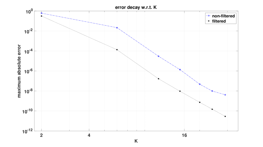
Figure 1: Approximand is $f_{1}(r,\theta,\varphi)=\frac{1}{0.0005^{\frac{17}{2}}}|r-1.0005|^{\frac{17}{2}}\cos^{4}\theta$. We fix $L=4$ and change $K$. We observe the algebraic decay of the error with respect to $K$ for both filtered and non-filtered hyperinterpolations.

To approximate the function $f_{1}$, we fix $L=4$ and vary the value of $K$. We observe the algebraic decay of the maximum absolute error with respect to $K$ for both filtered and non-filtered hyperinterpolations. See Fig. 1. The function $f_{1}$ is a $C^{8}([{r_{\mkern 0.0mu\mathrm{in}}},{r_{\mkern-2.5mu\mathrm{out}}}])$-function for a fixed angular variable.

As discussed in Section 5.3, for this reasonably smooth function $f_{1}$ we observe that non-filtered hyperinterpolation converges at a rate not much worse than the filtered case. For the filtered approximation, we observe an almost the same convergence rate, but with a smaller error. Since $f_{1}$ is in $C^{8}([{r_{\mkern 0.0mu\mathrm{in}}},{r_{\mkern-2.5mu\mathrm{out}}}])$, from Corollary 5.4 we expect that the logarithm of the error decays no slower than $-8\log_{10}K$. The experiment shows roughly $\log_{10}(\mathrm{error})\approx-10\log_{10}K$. This seems to show our result might not be sharp, but at least it is consistent with the experiment.

Next, we approximate the function $f_{2}$. We fix $K=2$, so that the radial part can be approximated exactly, and vary the value of $L$. See Fig. 2. We observe the algebraic decay of the error with respect to $K$. The function $f_{2}$ is a $C^{8}(S^{2})$-function for a fixed radial variable.

As discussed in Section 5.3, for this reasonably smooth function $f_{2}$ we observe that non-filtered hyperinterpolation converges at a rate not much worse than the filtered case. For the filtered approximation, we observe an almost the same convergence rate, but with a smaller error. Since $f_{2}$ is in $C^{8}(S^{2})$, from Corollary 5.4 we expect the logarithm of the error decays no slower than $-8\log_{10}L$. The experiment shows that roughly $\log_{10}(\mathrm{error})\approx-11\log_{10}L$, which is consistent with Corollary 5.4.

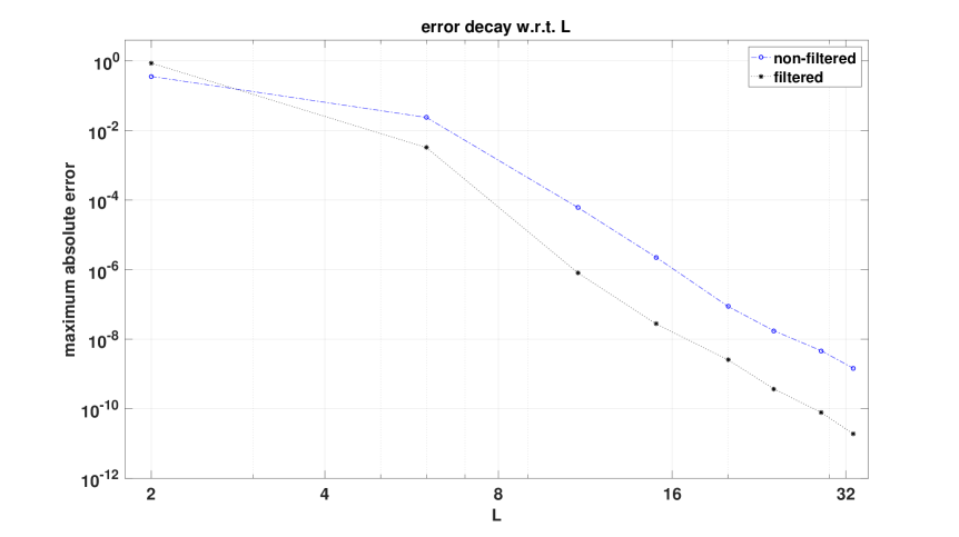
Figure 2: Approximand is $f_{2}(r,\theta,\varphi)=\frac{1}{0.001^{2}}(r-1)^{2}|\cos\theta|^{\frac{17}{2}}$. We fix $K=2$ and change $L$. We observe algebraic decay of the maximum absolute error with respect to $L$ for both filtered and non-filtered hyperinterpolations.

Next, we consider a non-smooth function which goes beyond the theory. It is constructed as a sum of following two functions. First, the Franke function $f_{\mathrm{Franke}}$ is a $C^{\infty}$-function defined by

$$f_{\mathrm{Franke}}(\bm{x})= 0.75\exp\left(-\frac{1}{4}((9x_{1}-2)^{2}+(9x_{2}-2)^{2}+(9x_{3}-2)^{2})\right)$$

$$+0.75\exp\left(-\frac{1}{49}((9x_{1}+1)^{2})-\frac{1}{10}(9x_{2}+1+9x_{3}+1)\right)$$

$$+0.5\exp\left(-\frac{1}{4}((9x_{1}-7)^{2}+(9x_{2}-3)^{2}+(9x_{3}-5)^{2})\right)$$

$$-0.2\exp\left(-(9x_{1}-4)^{2}-(9x_{2}-7)^{2}-(9x_{3}-5)^{2}\right),$$ (6.2)

for $\bm{x}=(x_{1},x_{2},x_{3})\in\mathbb{S}_{\varepsilon}$. Further, we define the cone function $f_{\mathrm{cone}}$ as follows

$$f_{\mathrm{cone}}(\bm{x}):=\begin{cases}1000\big{|}\|\bm{x}\|_{2}-1.0005\big{|}\Big{(}1-2\arccos\Big{(}\frac{\bm{x}}{\|\bm{x}\|_{2}}\cdot\bm{x}_{\mathrm{c}}\Big{)}\Big{)}&\bm{x}\in\mathcal{C}(\bm{x}_{\mathrm{c}})\\ 0&\text{otherwise},\end{cases}$$ (6.3)

where $\mathcal{C}(\bm{x}_{\mathrm{c}}):=\{\bm{x}\in\mathbb{S}_{\varepsilon}\mid\arccos(\bm{x}/\|\bm{x}\|_{2}\cdot\bm{x}_{\mathrm{c}}))\leq\frac{1}{2}\}$, and $\bm{x}_{\mathrm{c}}:=(-1/2,-1/2,1/\sqrt{2})\in S^{2}$. We approximate

$$f_{3}(\bm{x}):=f_{\mathrm{Franke}}(\bm{x})+f_{\mathrm{cone}}(\bm{x}).$$ (6.4)

Note that $f_{3}$ is not differentiable in the angular direction along the boundary of the spherical cap $\mathcal{C}(\bm{x}_{\mathrm{c}})$ nor at the centre of the cap, and in the radial direction at the midpoint of the interval $[1,1.001]$.

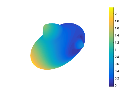
(a)

(b)

(c)

Figure 3: Top: function $f_{3}(1,\theta,\varphi)$. Left: hyperinterpolation error. Right: filtered hyperinterpolation error. $K=L=20$ is used.

We let $K=20$ and $L=20$ and observe the behaviour of the error. For a comparison, we again employ interpolation at the Chebyshev zeros in the radial direction, and hyperinterpolation on the sphere in the angular direction. We plot the exact functions at the top, the hyperinterpolation errors at the bottom left, the filtered hyperinterpolation error at the bottom right. Fig. 3–5 show the error on the spherical layers ($r=1,1.0005,1.001$), and Fig. 6 shows the error for the radial line $(-1/2r,-1/2r,1/\sqrt{2}r)$ $(r\in[1,1.001])$. We observe that the filtered hyperinterpolation errors are smaller, and more localised.

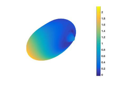
(a)

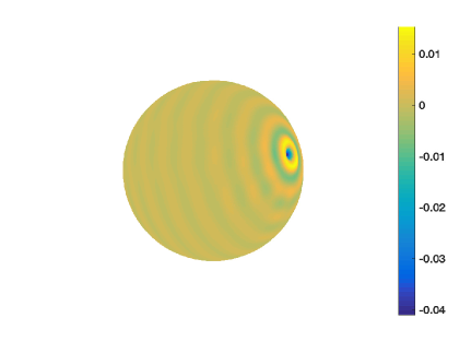
(b)

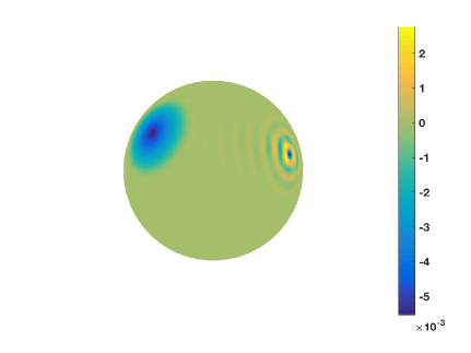
(c)

Figure 4: Top: function $f_{3}(1.0005,\theta,\varphi)$. Left: hyperinterpolation error. Right: filtered hyperinterpolation error. $K=L=20$ is used.

(a)

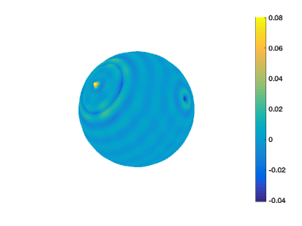
(b)

(c)

Figure 5: Top: function $f_{3}(1.001,\theta,\varphi)$. Left: hyperinterpolation error. Right: filtered hyperinterpolation error. $K=L=20$ is used.

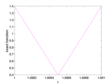
(a)

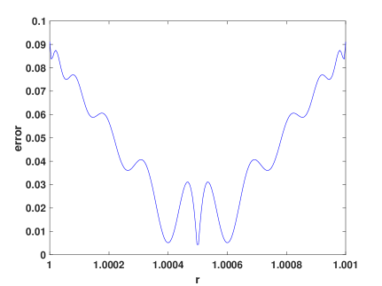
(b)

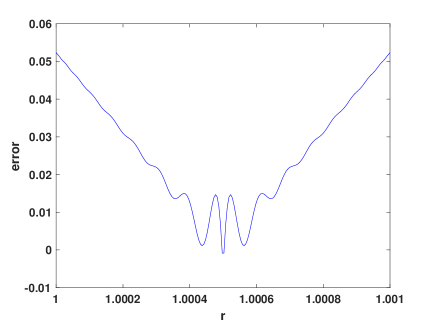
(c)

Figure 6: Top: function $f_{3}(r,\theta_{\mathrm{c}},\varphi_{\mathrm{c}})$, where $\theta_{\mathrm{c}}$ and $\varphi_{\mathrm{c}}$ are taken so that $(\sin\theta_{\mathrm{c}}\cos\varphi_{\mathrm{c}},\sin\theta_{\mathrm{c}}\sin\varphi_{\mathrm{c}},\cos\theta_{\mathrm{c}})=(-0.5,-0.5,1/\sqrt{2})$ Left: hyperinterpolation error. Right: filtered hyperinterpolation error.

7 Conclusion

We proposed a fully discrete filtered polynomial approximation on spherical shells. Our method is based on the filtered hyperinterpolation in the radial and angular directions. We provided an error analysis in terms of the supremum norm by reducing the approximation error to the best polynomial approximations. Numerical results are consistent with the theory.

References

[1]Wolfgang Bangerth, Juliane Dannberg, Rene Gassmöller and Timo Heister
“Computational modeling of convection in the Earth’s mantle”
In SIAM News49.2, 2016, pp. 1–3
[2]C. Canuto, M.Y. Hussaini, A. Quarteroni and T.A. Zang
“Spectral Methods Fundamentals in Single Domains”
Springer, 2006
[3]F. Dai and Y. Xu
“Polynomial approximation in Sobolev spaces on the unit
sphere and the unit ball”
In J. Approx. Theory163.10, 2011, pp. 1400–1418
DOI: 10.1016/j.jat.2011.05.001
[4]F. Dai and Y. Xu
“Approximation Theory and Harmonic Analysis on Spheres and
Balls”
Springer, 2013
DOI: 10.1007/978-1-4614-6660-4
[6]F. Filbir, H.N. Mhaskar and J. Prestin
“On a filter for exponentially localized kernels based on
Jacobi polynomials”
In J. Approx. Theory160.1-2, 2009, pp. 256–280
DOI: 10.1016/j.jat.2009.01.004
[7]Natasha Flyer, Grady B. Wright and Bengt Fornberg
“Radial basis function-generated finite differences: a
mesh-free method for computational geosciences”
In Handbook of GeomathematicsBerlin, Heidelberg: Springer, 2013, pp. 1–30
DOI: 10.1007/978-3-642-27793-1˙61-1
[8]Bengt Fornberg and Natasha Flyer
“Solving PDEs with radial basis functions”
In Acta Numer.24, 2015, pp. 215–258
[9] Geophysics Study Committee, Geophysics Research Forum, Commission on Physical Sciences, Mathematics and Resources and Commission on Physical Sciences, Mathematics, andΩApplications and Division on Engineering and Physical Sciences andΩNational Research Council
“The Earth’s Electrical Environment”
Washington, D.C: National Academies Press, 1986
URL: http://www.amazon.com/Earths-Electrical-Environment-Studies-Geophysics/dp/0309036801
[11]Jean Pierre Kahane and Yitzhak Katznelson
“Sur les ensembles de divergence des séries
trigonométriques”
In Studia Math.26, 1966, pp. 305–306
[12]Yoshihito Kazashi
“A fully discretised polynomial approximation on spherical
shells”
In GEM Int. J. Geomath.7.2, 2016, pp. 299–323
DOI: 10.1007/s13137-016-0084-1
[13]James C McWilliams
“Modeling the oceanic general circulation”
In Annu. Rev. Fluid Mech.28.1, 1996, pp. 215–248
[14]H. N. Mhaskar
“Polynomial operators and local smoothness classes on the
unit interval”
In J. Approx. Theory131.2, 2004, pp. 243–267
DOI: 10.1016/j.jat.2004.10.002
[15]H. N. Mhaskar and J. Prestin
“Polynomial frames: a fast tour”, Mod. Methods Math.
Nashboro Press, 2005, pp. 287–318
[16]Paul Nevai
“Géza Freud, orthogonal polynomials and Christoffel
functions. A case study”
In J. Approx. Theory48.1, 1986, pp. 3–167
DOI: 10.1016/0021-9045(86)90016-X
[17]Siegfried Pawelke
“Über die Approximationsordnung bei Kugelfunktionen und
algebraischen Polynomen”
In Tohoku Math. J.24.3, 1972, pp. 473–486
DOI: 10.2748/tmj/1178241489
[18]Pencho Petrushev and Yuan Xu
“Localized polynomial frames on the interval with Jacobi
weights”
In J. Fourier Anal. Appl.11.5, 2005, pp. 557–575
[19]M. J. D. Powell
“Approximation Theory and Methods”
Cambridge University Press, 1981, pp. x+339
[20]Ataru Sakuraba and Masaru Kono
“Effect of the inner core on the numerical solution of the
magnetohydrodynamic dynamo”
In Phys. Earth Planet. Inter.111.1-2, 1999, pp. 105–121
DOI: 10.1016/S0031-9201(98)00150-2
[22]Ian H. Sloan and Robert S. Womersley
“Constructive Polynomial Approximation on the Sphere”
In J. Approx. Theory103.1, 2000, pp. 91–118
DOI: 10.1006/jath.1999.3426
[23]Ian H. Sloan and Robert S. Womersley
“Filtered hyperinterpolation: a constructive polynomial
approximation on the sphere”
In GEM Int. J. Geomath.3.1, 2012, pp. 95–117
DOI: 10.1007/s13137-011-0029-7
[24]Gábor Szegő
“Orthogonal Polynomials”
American Mathematical Society, 1975, pp. xiii+432
[25]Paul J. Tackley
“Modelling compressible mantle convection with large
viscosity contrasts in a three-dimensional spherical shell using the yin-yang
grid”
In Phys. Earth Planet. Inter.171.1-4, 2008, pp. 7–18
DOI: 10.1016/j.pepi.2008.08.005
[26]Naum I͡Akovlevich Vilenkin
“Special Functions and the Theory of Group Representations”
American Mathematical Society, 1978, pp. 628
URL: http://books.google.co.jp/books?id=08hPoGgSQFIC
[27]Heping Wang and Ian H. Sloan
“On Filtered Polynomial Approximation on the Sphere”
In J. Fourier Anal. Appl.23.4, 2017, pp. 863–876
DOI: 10.1007/s00041-016-9493-7