Dispersion and viscous attenuation of capillary waves with finite amplitude

Abstract

We present a comprehensive study of the dispersion of capillary waves with finite amplitude, based on direct numerical simulations. The presented results show an increase of viscous attenuation and, consequently, a smaller frequency of capillary waves with increasing initial wave amplitude. Interestingly, however, the critical wavenumber as well as the wavenumber at which the maximum frequency is observed remain the same for a given two-phase system, irrespective of the wave amplitude. By devising an empirical correlation that describes the effect of the wave amplitude on the viscous attenuation, the dispersion of capillary waves with finite initial amplitude is shown to be, in very good approximation, self-similar throughout the entire underdamped regime and independent of the fluid properties. The results also shown that analytical solutions for capillary waves with infinitesimal amplitude are applicable with reasonable accuracy for capillary waves with moderate amplitude.

1 Introduction

Waves on fluid interfaces for which surface tension is the main restoring and dispersive mechanism, so-called capillary waves, play a key role in many physical phenomena, natural processes and engineering applications. Prominent examples are the heat and mass transfer between the atmosphere and the ocean (Witting, 1971; Szeri, 1997), capillary wave turbulence (Falcon et al., 2007; Deike et al., 2014; Abdurakhimov et al., 2015) and the stability of liquid and capillary bridges (Hoepffner and Paré, 2013; Castrejón-Pita et al., 2015).

The dispersion relation for a capillary wave with small amplitude on a fluid interface between two inviscid fluids is (Lamb, 1932)

$$\omega_{0}^{2}=\frac{\sigma k^{3}}{\tilde{\rho}}\ ,$$ (1)

where $\omega_{0}$ is the undamped angular frequency, $\sigma$ is the surface tension coefficient, $k$ is the wavenumber and $\tilde{\rho}=\rho_{\mathrm{a}}+\rho_{\mathrm{b}}$ is the relevant fluid density, where subscripts $\mathrm{a}$ and $\mathrm{b}$ denote properties of the two interacting bulk phases. The dispersion relation given in Eq. (1) is only valid for waves with infinitesimal amplitude (Lamb, 1932). In reality, however, capillary waves typically have a finite amplitude. Crapper (1957) was the first to provide an exact solution for progressive capillary waves of finite amplitude in fluids of infinite depth. The frequency of capillary waves with finite amplitude $a$ (measured from the equilibrium position to the wave crest or trough) and wavelength $\lambda$ is given as (Crapper, 1957)

$$\omega=\omega_{0}\,\left(1+\frac{\pi^{2}\,a^{2}}{\lambda^{2}}\right)^{-1/4}\ .$$ (2)

The solution of Crapper (1957) was extended to capillary waves on liquid films of finite depth by Kinnersley (1976) and to general gravity and capillary waves by Bloor (1978). However, these studies neglected viscous stresses, in order to make an analytical solution feasible.

Since capillary waves typically have a short wavelength (otherwise the influence of gravity also has to be considered) and because viscous stresses act preferably at small lengthscales (Lamb, 1932; Longuet-Higgins, 1992), understanding how viscous stresses affect the dispersion of capillary waves is crucial for a complete understanding of the associated processes and for optimising the related applications. Viscous stresses are known to attenuate the wave motion, with the frequency of capillary waves in viscous fluids being $\omega=\omega_{0}+i\Gamma$. This complex frequency leads to three damping regimes: the underdamped regime for $k<k_{\mathrm{c}}$, critical damping for $k=k_{\mathrm{c}}$ and the overdamped regime for $k>k_{\mathrm{c}}$. A wave with critical wavenumber $k_{\mathrm{c}}$ requires the shortest time to return to its equilibrium state without oscillating, with the real part of its complex angular frequency vanishing, $\mathrm{Re}(\omega)=0$. Critical damping, thus, represents the transition from the underdamped (oscillatory) regime, with $k<k_{\mathrm{c}}$ and $\mathrm{Re}(\omega)>0$, to the overdamped (non-oscillatory) regime, with $k>k_{\mathrm{c}}$ and $\mathrm{Re}(\omega)=0$. Based on the linearised Navier-Stokes equations, in this context usually referred to as the weak damping assumption, the dispersion relation of capillary waves in viscous fluids is given as (Levich, 1962; Landau and Lifshitz, 1966; Byrne and Earnshaw, 1979)

$$\omega_{0}^{2}+\left(i\omega+2\nu k^{2}\right)^{2}-4\nu^{2}k^{4}\sqrt{1+\frac{i\omega}{\nu k^{2}}}=0\ ,$$ (3)

where $\nu=\mu/\rho$ is the kinematic viscosity and $\mu$ is the dynamic viscosity. The damping rate based on Eq. (3) is $\Gamma=2\nu k^{2}$, applicable for $k\ll\sqrt{\omega_{0}/\nu}$ (Jeng et al., 1998). Note that Eq. (3) has been derived for a single fluid with a free surface (Levich, 1962). Previous analytical and numerical studies showed that the damping coefficient $\Gamma$ is not a constant, but is dependent on the wavenumber and changes significantly throughout the underdamped regime (Jeng et al., 1998; Denner, 2016). Denner (2016) recently proposed a consistent scaling for small-amplitude capillary waves in viscous fluids, which leads to a self-similar characterisation of the frequency dispersion of capillary waves in the entire underdamped regime. The results reported by Denner (2016) also suggest that the weak damping assumption is not appropriate when viscous stresses dominate the dispersion of capillary waves, close to critical damping. With regards to finite-amplitude capillary waves in viscous fluids, the interplay between wave amplitude and viscosity as well as the effect of the amplitude on the frequency and critical wavelength have yet to be studied and quantified.

In this article, direct numerical simulation (DNS) is applied to study the dispersion and viscous attenuation of freely-decaying capillary waves with finite amplitude in viscous fluids. The presented results show a nonlinear increase in viscous attenuation and, hence, a lower frequency for an increasing initial amplitude of capillary waves. Nevertheless, the critical wavenumber for a given two-phase system is found to be independent of the initial wave amplitude and is accurately predicted by the harmonic oscillator model proposed by Denner (2016). An empirical correction to the characteristic viscocapillary timescale is proposed that leads to a self-similar solution for the dispersion of finite-amplitude capillary waves in viscous fluids.

In Sect. 2 the characterisation of capillary waves is discussed and Sect. 3 describes the computational methods used in this study. In Sect. 4, the dispersion of capillary waves with finite amplitude is studied and Sect. 5 analyses the validity of linear wave theory based on an infinitesimal wave amplitude. The article is summarised and conclusions are drawn in Sect. 6.

2 Characterisation of capillary waves

Assuming that no gravity is acting, the fluids are free of surfactants and inertia is negligible, only two physical mechanisms govern the dispersion of capillary waves; surface tension (dispersion) and viscous stresses (dissipation). The main characteristic of a capillary wave in viscous fluids is its frequency

$$\omega=\omega_{0}+i\Gamma=\omega_{0}\,\sqrt{1-\zeta^{2}}\ ,$$ (4)

with $\zeta=\Gamma/\omega_{0}$ being the damping ratio. In the underdamped regime (for $k<k_{\mathrm{c}}$) the damping ratio is $\zeta<1$, $\zeta=1$ for critical damping ($k=k_{\mathrm{c}}$) and $\zeta>1$ in the overdamped regime (for $k>k_{\mathrm{c}}$). As recently shown by Denner (2016), the dispersion of capillary waves can be consistently parameterised by the critical wavenumber $k_{\mathrm{c}}$ together with an appropriate timescale.

The wavenumber at which capillary waves are critically damped, the so-called critical wavenumber, is given as (Denner, 2016)

$$k_{\mathrm{c}}=\frac{2^{2/3}}{l_{\mathrm{vc}}}\,\left(1.0625-\beta\right)\ ,$$ (5)

where the viscocapillary lengthscale is

$$l_{\mathrm{vc}}=\frac{\tilde{\mu}^{2}}{\sigma\,\tilde{\rho}}\ ,$$ (6)

with $\tilde{\mu}=\mu_{\mathrm{a}}+\mu_{\mathrm{b}}$, and

$$\beta=\frac{\rho_{\mathrm{a}}\rho_{\mathrm{b}}}{\tilde{\rho}^{2}}\frac{\nu_{\mathrm{a}}\nu_{\mathrm{b}}}{\tilde{\nu}^{2}}$$ (7)

is a property ratio, with $\tilde{\nu}=\nu_{\mathrm{a}}+\nu_{\mathrm{b}}$. Note that $l_{\mathrm{vc}}$ follows from a balance of capillary and viscous timescales (Denner, 2016). Based on the governing mechanisms, the characteristic timescale of the dispersion of capillary waves is the viscocapillary timescale (Denner, 2016)

$$t_{\mathrm{vc}}=\frac{\tilde{\mu}^{3}}{\sigma^{2}\,\tilde{\rho}}\ .$$ (8)

Defining the dimensionless wavenumber as $\hat{k}=k/k_{\mathrm{c}}$ and the dimensionless frequency as $\hat{\omega}=\omega t_{\mathrm{vc}}$ results in a self-similar characterisation of the dispersion of capillary waves with small (infinitesimal) amplitude (Denner, 2016), i.e. there exists a single dimensionless frequency $\hat{\omega}$ for every dimensionless wavenumber $\hat{k}$.

3 Computational methods

The incompressible flow of isothermal, Newtonian fluids is governed by the momentum equations

$$\frac{\partial u_{i}}{\partial t}+u_{j}\frac{\partial u_{i}}{\partial x_{j}}=-\frac{1}{\rho}\frac{\partial p}{\partial x_{i}}+\frac{\partial}{\partial x_{j}}\left[\nu\left(\frac{\partial u_{i}}{\partial x_{j}}+\frac{\partial u_{j}}{\partial x_{i}}\right)\right]+\frac{f_{\mathrm{\sigma},i}}{\rho}$$ (9)

and the continuity equation

$$\frac{\partial u_{i}}{\partial x_{i}}=0\ ,$$ (10)

where $\boldsymbol{x}\equiv(x,y,z)$ denotes a Cartesian coordinate system, $t$ represents time, $\boldsymbol{u}$ is the velocity, $p$ is the pressure and $\boldsymbol{f}_{\sigma}$ is the volumetric force due to surface tension acting at the fluid interface. The hydrodynamic balance of forces acting at the fluid interface is given as Levich and Krylov (1969)

$$\left(p_{\mathrm{a}}-p_{\mathrm{b}}\right.+\left.\sigma\,\kappa\right)\hat{m}_{i}=\left[\mu_{\mathrm{a}}\left(\left.\frac{\partial u_{i}}{\partial x_{j}}\right|_{\mathrm{a}}+\left.\frac{\partial u_{j}}{\partial x_{i}}\right|_{\mathrm{a}}\right)\right.-\left.\mu_{\mathrm{b}}\left(\left.\frac{\partial u_{i}}{\partial x_{j}}\right|_{\mathrm{b}}+\left.\frac{\partial u_{j}}{\partial x_{i}}\right|_{\mathrm{b}}\right)\right]\hat{m}_{j}-\frac{\partial\sigma}{\partial x_{i}}\ ,$$ (11)

where $\kappa$ is the curvature and $\boldsymbol{\hat{m}}$ is the unit normal vector (pointing into fluid b) of the fluid interface. In the current study the surface tension coefficient $\sigma$ is taken to be constant and, hence, $\nabla\sigma=0$. Delgado-Buscalioni et al. (2008) performed extensive molecular dynamics simulations, showing that hydrodynamic theory is applicable to capillary waves in the underdamped regime as well as at critical damping.

3.1 DNS methodology

The governing equations are solved numerically in a single linear system of equations using a coupled finite-volume framework with collocated variable arrangement (Denner and van Wachem, 2014), resolving all relevant scales in space and time. The momentum equations, Eq. (9), are discretised using a Second-Order Backward Euler scheme for the transient term and convection is discretised using central differencing (Denner, 2013). The continuity equation, Eq. (10), is discretised using the momentum-weighted interpolation method for two-phase flows proposed by Denner and van Wachem (2014), providing an accurate and robust pressure-velocity coupling.

The Volume-of-Fluid (VOF) method (Hirt and Nichols, 1981) is adopted to capture the interface between the immiscible bulk phases. The local volume fraction of both phases is represented by the colour function $\gamma$, with the interface located in mesh cells with a colour function value of $0<\gamma<1$. The local density $\rho$ and viscosity $\mu$ are interpolated using an arithmetic average based on the colour function $\gamma$ (Denner and van Wachem, 2014), e.g. $\rho(\boldsymbol{x})=\rho_{\mathrm{a}}[1-\gamma(\boldsymbol{x})]+\rho_{\mathrm{b}}\gamma(\boldsymbol{x})$ for density. The colour function $\gamma$ is advected by the linear advection equation

$$\frac{\partial\gamma}{\partial t}+u_{i}\frac{\partial\gamma}{\partial x_{i}}=0\ ,$$ (12)

which is discretised using a compressive VOF method (Denner and van Wachem, 2014).

Surface tension is modelled as a surface force per unit volume, described by the CSF model (Brackbill et al., 1992) as $\boldsymbol{f}_{s}=\sigma\,\kappa\,\nabla\gamma$. The interface curvature is computed as $\kappa=h_{xx}/\left(1+h_{x}^{2}\right)^{3/2}$, where $h_{x}$ and $h_{xx}$ represent the first and second derivatives of the height function $h$ of the colour function with respect to the $x$-axis of the Cartesian coordinate system, calculated by means of central differences. No convolution is applied to smooth the colour function field or the surface force (Denner and van Wachem, 2013).

A standing capillary wave with wavelength $\lambda$ and initial amplitude $a_{0}$ in four different two-phase systems is simulated. The fluid properties of the considered cases, which have previously also been considered in the study on the dispersion of small-amplitude capillary waves in viscous fluids by Denner (2016), are given in Table 1. The computational domain, sketched in Fig. 1, has the dimensions $\lambda\times 3\lambda$ and is represented by an equidistant Cartesian mesh with mesh spacing $\Delta x=\lambda/100$, which has previously been shown to provide an adequate spatial resolution Denner (2016). The applied computational time-step is $\Delta t=(200\,\omega_{0})^{-1}$, which satisfies the capillary time-step constraint (Denner and van Wachem, 2015) and results in a Courant number of $\mathit{Co}=\Delta t\,|\boldsymbol{u}|/\Delta x<10^{-2}$. The domain boundaries oriented parallel to the interface are treated as free-slip walls, whereas periodic boundary conditions are applied at the other domain boundaries. The flow field is initially stationary and no gravity is acting.

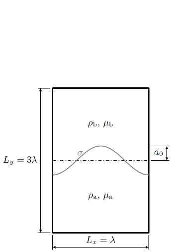
Figure 1: Sketch (not to scale) of the two-dimensional computational domain with a standing capillary wave with amplitude $a_{0}$ indicated in grey.

Table 1: Fluid properties and property ratio $\beta$ of the considered cases.

Case	$\rho_{\mathrm{a}}\ [\mathrm{kg}\,\mathrm{m}^{-3}]$	$\mu_{\mathrm{a}}\ [\mathrm{Pa}\,\mathrm{s}]$	$\rho_{\mathrm{b}}\ [\mathrm{kg}\,\mathrm{m}^{-3}]$	$\mu_{\mathrm{b}}\ [\mathrm{Pa}\,\mathrm{s}]$	$\sigma\ [\mathrm{N}\,\mathrm{m}^{-1}]$	$\beta$
A	$5.0$	$0.7$	$5.0$	$0.7$	$10^{-3}$	$6.250\times 10^{-2}$
B	$800.0$	$0.319$	$1450.0$	$2.0$	$7.5\times 10^{-4}$	$3.986\times 10^{-2}$
C	$2.0$	$0.01$	$200.0$	$1.0$	$2.1\times 10^{-2}$	$2.451\times 10^{-3}$
D	$1.205$	$1.82\times 10^{-5}$	$1000.0$	$0.001$	$10^{-5}$	$7.001\times 10^{-5}$

3.2 Analytical initial-value solution

The analytical initial-value solution (AIVS) for small-amplitude capillary waves in viscous fluids, as proposed by Prosperetti (1976, 1981) based on the linearised Navier-Stokes equations, for the special cases of a single fluid with a free-surface (i.e. $\rho_{\textrm{b}}=\mu_{\textrm{b}}=0$) (Prosperetti, 1976) and for two-phase systems with equal bulk phases of equal kinematic viscosity (i.e. $\nu_{\textrm{a}}=\nu_{\textrm{b}}$) (Prosperetti, 1981) is considered as reference solution. Since the AIVS is based on the linearised Navier-Stokes equations, it is only valid in the limit of infinitesimal wave amplitude $a_{0}\rightarrow 0$. In the present study, the AIVS is computed at time intervals $\Delta t=(200\,\omega_{0})^{-1}$, i.e. with $200$ solutions per undamped period, which provides a sufficient temporal resolution of the evolution of the capillary wave.

3.3 Validation

The dimensionless frequency $\hat{\omega}=\omega t_{\mathrm{vc}}$ as a function of dimensionless wavenumber $\hat{k}=k/k_{\mathrm{c}}$ for Case A with initial wave amplitude $a_{0}=0.01\lambda$ is shown in Fig. 2a, where the results obtained with the DNS methodology described in Sect. 3.1 are compared against AIVS, see Sect. 3.2, as well as results obtained with the open-source DNS code Gerris (Popinet, 2003, 2009). The applied DNS methodology is in very good agreement with the results obtained with Gerris and is excellent agreement with the analytical solution up to $\hat{k}\approx 0.9$. For $\hat{k}>0.9$ the very small amplitude at the first extrema ($|a_{1}|\sim 10^{-6}$) is indistinguishable from the error caused by the underpinning modelling assumption and numerical discretisation errors. Hence, the applied numerical method can provide accurate and reliable results for $\hat{k}\leq 0.9$, as previously reported in Ref. (Denner, 2016). Figure 2b shows DNS result of the dimensionless frequency as a function of dimensionless wavenumber for Case A with an initial amplitude of $a_{0}=0.1\lambda$, compared against results obtained with Gerris, exhibiting a very good agreement. Note that Gerris has previously been successfully applied to a variety of related problems, such as capillary wave turbulence Deike et al. (2014, 2015) and capillary-driven jet breakup (Moallemi et al., 2016).

(a) $a_{0}=0.01\lambda$

(b) $a_{0}=0.1\lambda$

Figure 2: Dimensionless frequency $\hat{\omega}$ as a function of dimensionless wavenumber $\hat{k}$ obtained with the applied DNS methodology and the open-source code Gerris for initial wave amplitudes $a_{0}=0.01\lambda$ and $a_{0}=0.1\lambda$.

4 Dispersion and damping of finite-amplitude capillary waves

The damping ratio $\zeta$ as a function of dimensionless wavenumber $\hat{k}$ for Cases A and D with different initial wave amplitudes $a_{0}$ is shown in Fig. 3. The damping ratio increases with increasing amplitude for any given wavenumber $\hat{k}<1$. This trend is particularly pronounced for smaller wavenumbers, i.e. longer wavelength. Irrespective of the initial amplitude $a_{0}$ of the capillary wave, however, critical damping ($\zeta=1$) is observed at $\hat{k}=k/k_{\mathrm{c}}=1$, with $k_{\mathrm{c}}$ defined by Eq. (5). Hence, the critical wavenumber and, consequently, the characteristic lengthscale $l_{\mathrm{vc}}$ remain unchanged for different initial amplitudes of the capillary wave.

(a) Case A

(b) Case D

Figure 3: Damping ratio $\zeta$ as a function of dimensionless wavenumber $\hat{k}$ for Cases A and D with different initial wave amplitudes $a_{0}$.

As a result of the increased damping for capillary waves with larger initial amplitude, the frequency of capillary waves with large initial amplitude is lower than the frequency of capillary waves with the same wavenumber but smaller initial amplitude, as observed in Fig. 4, which shows the dimensionless frequency $\hat{\omega}=\omega t_{\textrm{vc}}$ as a function of dimensionless wavenumber $\hat{k}=k/k_{\textrm{c}}$ for Cases A and D with different initial wave amplitudes. Interestingly, the wavenumber at which the maximum frequency is observed, $k_{\textrm{m}}\approx 0.751k_{\textrm{c}}$, is unchanged by the initial amplitude of the capillary wave. This concurs with the earlier observation that the critical wavenumber is not dependent on the initial wave amplitude. Furthermore, comparing Figs. 4a and 4b suggests that there exists a single dimensionless frequency $\hat{\omega}=\omega t_{\textrm{vc}}$ for any given dimensionless wavenumber $\hat{k}$ and initial wave amplitude $a_{0}$.

(a) Case A

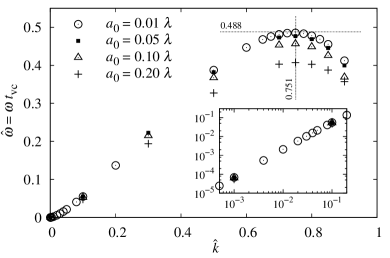
(b) Case D

Figure 4: Dimensionless frequency $\hat{\omega}=\omega t_{\mathrm{vc}}$ as a function of dimensionless wavenumber $\hat{k}$ for Cases A and D with different initial wave amplitudes $a_{0}$.

Based on the DNS results for the considered cases and different initial amplitudes, an amplitude-correction to the viscocapillary timescale $t_{\textrm{vc}}$ can be devised. Figure 5 shows the correction factor $C=t_{\textrm{vc}}^{\ast}/t_{\textrm{vc}}$, where $t_{\textrm{vc}}^{\ast}$ is the viscocapillary timescale obtained from DNS results with various initial amplitudes, as a function of the dimensionless initial amplitude $\hat{a}_{0}=a_{0}/\lambda$. This correction factor is well approximated at $\hat{k}=0.75$ by the correlation

$$C\approx-4.5\,\hat{a}_{0}^{3}+5.3\,\hat{a}_{0}^{2}+0.18\,\hat{a}_{0}+1\ ,$$ (13)

as seen in Fig. 5. The amplitude-corrected viscocapillary timescale then readily follows as

$$t_{\textrm{vc}}^{\ast}\approx C\,t_{\textrm{vc}}\ .$$ (14)

Thus, the change in frequency as a result of a finite initial wave amplitude is independent of the fluid properties. Note that this correction is particularly accurate for moderate wave amplitudes of $a_{0}\lesssim 0.1\lambda$.

Figure 5: Correction factor $C$ of the amplitude-corrected viscocapillary timescale $t_{\mathrm{vc}}^{\ast}$ as a function of dimensionless initial wave amplitude $\hat{a_{0}}=a_{0}/\lambda$ for different cases. The solid line shows the correlation for $C$ defined in Eq. (13).

By redefining the dimensionless frequency $\hat{\omega}^{\ast}=\omega t_{\textrm{vc}}^{\ast}$ with the amplitude-corrected viscocapillary timescale $t_{\textrm{vc}}^{\ast}$ as defined in Eq. (14), a (approximately) self-similar solution of the dispersion of capillary waves with initial wave amplitude $a_{0}$ can be obtained, as seen in Fig. 6. Thus, for every dimensionless wavenumber $\hat{k}$ there exists, in good approximation, only one dimensionless frequency $\hat{\omega}^{\ast}$. The maximum frequency is $\hat{\omega}_{\textrm{m}}^{\ast}\approx 0.488$ at $\hat{k}_{\textrm{m}}\approx 0.751$, as previously reported for small-amplitude capillary waves (Denner, 2016).

(a) $a_{0}=0.05\lambda$

(b) $a_{0}=0.2\lambda$

Figure 6: Dimensionless frequency $\hat{\omega}^{\ast}=\omega t_{\mathrm{vc}}^{\ast}$, with $t_{\mathrm{vc}}^{\ast}$ being the amplitude-corrected viscocapillary timescale, as a function of dimensionless wavenumber $\hat{k}$ for all considered cases with initial wave amplitude $a_{0}=0.05\lambda$ and $a_{0}=0.2\lambda$.

5 Validity of linear wave theory

As observed and discussed in the previous section, an increasing initial wave amplitude results in a lower frequency of the capillary wave. The influence of the amplitude is small if $\tilde{\mu}=0$. According to the analytical solution derived by Crapper (1957) for inviscid fluids, see Eq. (2), the frequency error

$$\varepsilon(\hat{k},\hat{a}_{0})=\frac{|\omega_{\mathrm{AIVS}}(\hat{k})-\omega(\hat{k},\hat{a}_{0})|}{{\omega}_{\mathrm{AIVS}}(\hat{k})}\ ,$$ (15)

where $\omega_{\mathrm{AIVS}}$ is the frequency according to the AIVS solution, is $\varepsilon=0.06\%$ for $a_{0}=0.05\lambda$ and $\varepsilon=2.32\%$ for $a_{0}=0.10\lambda$.

The influence of the initial wave amplitude on the frequency of capillary waves increases significantly in viscous fluids. As seen in Fig. 7a for Case A with $\hat{k}=0.01$, the time to the first extrema increases noticeably for increasing initial wave amplitude $a_{0}$. However, this frequency shift diminishes for subsequent extrema as the wave decays rapidly and the wave amplitude reduces. The frequency error $\varepsilon$ associated with a finite initial wave amplitude, shown in Fig. 7b, is approximately constant for the considered range of dimensionless wavenumbers and is, hence, predominantly a function of the wave amplitude. For an initial amplitude of $a_{0}=0.05\lambda$ the frequency error is $\varepsilon\approx 2.5\%$, as observed in Fig. 7b, and rises to $\varepsilon\approx 7.5\%$ for $a_{0}=0.10\lambda$.

(a) Evolution of the dimensionless amplitude $a/a_{0}$ as a function of dimensionless time $\tau=t\,\omega_{0}$ for Case A with $\hat{k}=0.01$. The insets highlight particular time intervals.

(b) Comparison of the frequency error $\epsilon$ of Case A as a function of the dimensionless wavenumber $\hat{k}$ for different initial wave amplitudes $a_{0}$.

Figure 7: Changes in the evolution of the capillary wave amplitude for different initial wave amplitudes and frequency error associated with different initial wave amplitudes as a function of dimensionless wavenumber $\hat{k}$.

6 Conclusions

The dispersion and viscous attenuation of capillary waves is considerably affected by the wave amplitude. Using direct numerical simulation in conjunction with an analytical solution for small-amplitude capillary waves, we have studied the frequency and the damping ratio of capillary waves with finite amplitude in the underdamped regime, including critical damping.

The presented numerical results show that capillary waves with a given wavenumber experience a larger viscous attenuation and exhibit a lower frequency if their initial amplitude is increased. Interestingly, however, the critical wavenumber of a capillary wave in a given two-phase system is independent of the wave amplitude. Similarly, the wavenumber at which the maximum frequency of the capillary wave is observed remains unchanged by the wave amplitude, although the maximum frequency depends on the wave amplitude, with a smaller maximum frequency for increasing wave amplitude. Consequently, the viscocapillary lengthscale $l_{\mathrm{vc}}$ is independent of the wave amplitude and $k\sim l_{\textrm{vc}}^{-1}$ irrespective of the wave amplitude. The reported reduction in frequency for increasing wave amplitude has been consistently observed for all considered two-phase systems, meaning that a larger amplitude leads to an increase of the viscocapillary timescale $t_{\mathrm{vc}}$. The viscocapillary timescale has been corrected for the wave amplitude with an empirical correlation, which leads to an approximately self-similar solution of the dispersion of capillary waves with finite amplitude in arbitrary viscous fluids.

Comparing the frequency of finite-amplitude capillary waves with the analytical solution for infinitesimal amplitude, we found that the analytical solution based on the infinitesimal-amplitude assumption is applicable with reasonable accuracy ($\varepsilon\lesssim 2.5\%$) for capillary waves with an amplitude of $a_{0}\lesssim 0.05\lambda$.