Charge states and FIP bias of the solar wind from coronal holes, active regions, and quiet Sun

Abstract

Connecting in-situ measured solar-wind plasma properties with typical regions on the Sun can provide an effective constraint and test to various solar wind models. We examine the statistical characteristics of the solar wind with an origin in different types of source regions. We find that the speed distribution of coronal hole (CH) wind is bimodal with the slow wind peaking at $\sim$400 km s^-1 and a fast at $\sim$600 km s^-1. An anti-correlation between the solar wind speeds and the O⁷⁺/O⁶⁺ ion ratio remains valid in all three types of solar wind as well during the three studied solar cycle activity phases, i.e. solar maximum, decline and minimum. The $N_{Fe}/N_{O}$ range and its average values all decrease with the increasing solar wind speed in different types of solar wind. The $N_{Fe}/N_{O}$ range (0.06–0.40, FIP bias range 1–7) for AR wind is wider than for CH wind (0.06–0.20, FIP bias range 1–3) while the minimum value of $N_{Fe}/N_{O}$ ($\sim$ 0.06) does not change with the variation of speed, and it is similar for all source regions. The two-peak distribution of CH wind and the anti-correlation between the speed and O⁷⁺/O⁶⁺ in all three types of solar wind can be explained qualitatively by both the wave-turbulence-driven (WTD) and reconnection-loop-opening (RLO) models, whereas the distribution features of $N_{Fe}/N_{O}$ in different source regions of solar wind can be explained more reasonably by the RLO models.

1 Introduction

It is common knowledge that the in-situ solar wind has two basic components: a steady fast ($\sim$800 km s^-1) and a variable slow ($\sim$400 km s^-1) component (e.g. Schwenn, 2006, and the references therein). While it is widely accepted that the fast solar wind (FSW) originates in coronal holes (Krieger et al., 1973; Zirker, 1977; Gosling & Pizzo, 1999), the source regions of the slow solar wind (SSW) are still poorly understood. One of the sources of the SSW has been linked to sources at the edges of active regions (e.g. Kojima et al., 1999; Sakao et al., 2007; Culhane et al., 2014, etc.) and it is also believed that the SSW originates in the quiet Sun (e.g. Woo & Habbal, 2000; Feldman et al., 2005; Fu et al., 2015).

Intuitively, identification of wind sources can be done by tracing wind parcels back to the Sun. By applying a potential-field-source-surface (PFSS) model, Luhmann et al. (2002) mapped a low latitude solar wind back to the photosphere for nearly three solar activity cycles. They showed, for instance, that polar coronal holes contribute to the solar wind only over about the half solar cycle, while for the rest of the time the low-latitude solar wind originates from “isolated low-latitude and midlatitude coronal holes or polar coronal hole extensions that have a flow character distinct from that of the large polar hole flows”. Using a standard two-step mapping procedure, Neugebauer et al. (2002) traced solar wind parcels back to the solar surface for four Carrington rotations during a solar maximum phase. The solar wind was divided into two categories: coronal hole and active region wind, and their statistical parameters were analyzed separately. The authors reported that the O⁷⁺/O⁶⁺ ion ratio is lower for the coronal-hole wind in comparison to the active-region wind. Fu et al. (2015) traced the solar wind back to its sources and classified the solar wind by the type of the source region, i.e. active region (AR), quiet Sun (QS) and coronal hole (CH) wind. They found that the fractions occupied by each type of solar wind change with the solar cycle activity and established that the quiet Sun regions are an important source of the solar wind during the solar minimum phase.

Alternatively, wind sources can be determined by examining in-situ charge states and elemental abundances. For the former, the charge states of species such as oxygen and carbon are regarded as a telltale signature of the solar wind sources. For example, the density ratio of n(O⁷⁺) to n(O⁶⁺) (i.e. ionic charge state ratio, hereafter O⁷⁺/O⁶⁺) does not vary with the distance beyond several solar radii above the solar surface, and, therefore, it reflects the electron temperature in the coronal sources (Owocki et al., 1983; Buergi & Geiss, 1986). As the temperatures in different source regions are different, therefore, the source regions can be identified by the charge states detected in situ (Zhao et al., 2009; Landi et al., 2012). The first ionization potential (FIP) effect describes the element anomalies in the upper solar atmosphere and the solar wind (especially in the SSW), i.e. the abundance increase of elements with a FIP of less than 10 eV (e.g., Mg, Si, and Fe) to those with a higher FIP (e.g., O, Ne, and He). The in-situ measured FIP bias is usually represented by $N_{Fe}/N_{O}$  and it can be expressed as

$$FIP~{}bias=\frac{(N_{Fe}/N_{O})_{solar~{}wind}}{(N_{Fe}/N_{O})_{photosphere}},$$ (1)

where $N_{Fe}/N_{O}$ is the abundance ratio of iron (Fe) and oxygen (O). In the slow wind the FIP bias is $\sim$3, while in the fast streams it is found to be smaller but still above 1 (von Steiger et al., 2000). As the FIP bias in coronal holes, the quiet Sun, and active regions has significant differences, the solar wind detected in situ can be linked to those source regions (e.g., Feldman et al., 2005; Laming, 2015, and the references thererin). In the present study, we only present the in-situ measurements of $N_{Fe}/N_{O}$ that can easily be translated to a FIP bias by considering $N_{Fe}/N_{O}$ in the photosphere to be a constant at $\sim$0.06 (Asplund et al., 2009).

Two theoretical frameworks, the wave-turbulence-driven (WTD) models and the reconnection-loop-opening (RLO) models, have been proposed to account for the observational results. In the WTD models, the magnetic funnels are jostled by the photosphere convection, and waves are produced that propagate into the upper atmosphere. These waves can dissipate to heat and accelerate the nascent solar wind (Hollweg, 1986; Wang & Sheeley, 1991; Cranmer et al., 2007; Verdini et al., 2009). In the RLO models the magnetic-field line of loops reconnect with open field lines and during this process mass and energy are released (Fisk et al., 1999; Fisk, 2003; Schwadron & McComas, 2003; Woo et al., 2004; Fisk & Zurbuchen, 2006). For more details on these two classes of models please see the review by Cranmer (2009). There are two important differences between the two models. First, in the WTD models the plasma escapes directly along open magnetic-field lines, whereas in the RLO models the plasma is released from closed loops through magnetic reconnection. Second, in the WTD models the speed of the solar wind is determined by the super radial expansion (Wang & Sheeley, 1990) and curvature degree (Li et al., 2011) of the open magnetic-field lines. In the RLO models, the speed of the solar wind depends on the temperature of the loops that reconnect with the open magnetic-field lines with hotter loops producing slow wind, and cooler loops producing fast wind (Fisk, 2003).

Observations can be used to test any of the above mentioned models. For this purpose, the following three questions need to be addressed. First, where do the two components (a steady fast component and a variable slow portion (Schwenn, 2006)) of the solar wind originate from? Second, why does the charge state anti-correlate with the solar wind speed (Geiss et al., 1995; von Steiger et al., 2000; Gloeckler et al., 2003; Wang & Sheeley, 2003; Wang et al., 2009)? Third, why is the FIP bias (FIP bias value range) higher (wider) in the slow solar wind than in the fast wind (Geiss et al., 1995; von Steiger et al., 2000; Abbo et al., 2016)?

Traditionally, solar wind is classified by its speeds. The speed, however, is not the only characteristic feature of the solar wind (Antiochos et al., 2012; Abbo et al., 2016). The plasma properties and magnetic-field structures can be significantly different depending on the solar regions, i.e. coronal holes, quiet Sun, and active regions. The differences in the source regions would then influence the solar wind streams they generate (Feldman et al., 2005). Therefore, connecting in-situ measured solar-wind plasma properties with typical regions on the Sun can provide an effective constraint and test to various solar wind models (Landi et al., 2014). In an earlier study, we classified the solar wind by the source region type (CHs, QS, and ARs) (Fu et al., 2015). Here, we analyze the relationship between in-situ solar wind parameters and source regions in different phases of the solar cycle activity. We aim at answering the following outstanding questions: 1) Are there any differences in the speed, O⁷⁺/O⁶⁺, and $N_{Fe}/N_{O}$ distributions of the different types of solar wind, i.e. AR, QS and CH? 2) Is the anti-correlation between the solar wind speed and O⁷⁺/O⁶⁺ charge state still valid for each type of solar wind? 3) What are the characteristics of the distribution in speed and $N_{Fe}/N_{O}$ space for the different types of solar wind? We also discuss our new results in the light of the WTD and RLO models.

The paper is organized as follows. In Section 2 we describe the data and the analysis methods. The statistical results are discussed in Section 3. The summary and concluding remarks are given in Section 4.

2 Data and Analysis

In Fu et al. (2015), the source regions were categorized into three groups: CHs, ARs, and QS, and the wind streams originating from these regions were given the corresponding names CH wind, AR wind, and QS wind, respectively. We used hourly averaged solar wind speeds measured by the Solar Wind Electron, Proton, and Alpha Monitor onboard the Advanced Composition Explorer (ACE, Stone et al., 1998). The charge state O⁷⁺/O⁶⁺ and FIP bias $N_{Fe}/N_{O}$  (also hourly averaged) were recorded by the Solar Wind Ion Composition Spectrometer, ( SWICS/ACE Gloeckler et al., 1998). In the present study we are only interested in the non-transient solar wind, and therefore, the intervals occupied by Interplanetary Coronal Mass Ejections (ICMEs) were excluded. We used the method suggested by Richardson & Cane (2004) where charge state O⁷⁺/O⁶⁺ exceeding $6.008exp(-0.00578v)$ ($v$ is the ICME speed) were discarded. In this study, the threshold for FSW and SSW is chosen as 500 km s^-1 (Fu et al., 2015; Abbo et al., 2016).

The two-step mapping procedure (Neugebauer et al., 1998, 2002) was applied to trace the solar wind parcels back to the solar surface. The footpoints were then placed on the EUV images observed by the Extreme-ultraviolet Imaging Telescope (EIT, Delaboudinière et al., 1995) and the photospheric magnetograms taken by the Michelson Doppler imager (MDI, Scherrer et al. 1995) onboard SoHO (Solar and Heliospheric Observatory, Domingo et al., 1995). Here, the EIT 284 Å passband was used as coronal holes are best distinguishable there.

The scheme for classifying the source regions is illustrated in the top panels (a–d) of Figure 1 where the footpoint locations (red crosses) are overplotted on the EIT images (a1, b1, c1, d1) and the photospheric magnetograms (a2, b2, c2, d2). The wind with footpoints located within CHs is classified as “CH wind”. A quantitative approach which follows that of Krista & Gallagher (2009) for identifying coronal hole boundaries is implemented. In this approach, a rectangular box which includes apparently dark area and its brighter surrounding area is chosen. There would be a multipeak distribution for its intensity histogram (see Figure 3 in Krista & Gallagher (2009) and Figure 2 in Fu et al. (2015)). The minimum between the first two peaks was defined as the threshold for the CH boundary (see the green contours in Figure 1, a1–d1). This scheme can define CH boundaries more objectively and it is not influenced by the emission variation of the corona with the solar activity. The definition of the AR wind relies on the magnetic field strength at photospheric level and corresponds to magnetically concentrated areas (MCAs). MCAs conform an area defined by the value of contour levels that are 1.5–4 times the mean of the radial component of the photospheric magnetic field. We found that the morphology of MCA is not sensitive to contour levels if it is in the above mentioned range. This means that the MCAs have a strong spatial gradient of the radial magnetic-field component. The defined MCAs encompass all active regions numbered by NOAA as given by the solarmonitor . However, not all MCAs correspond to an AR numbered by NOAA. As CH boundaries are defined quantitatively, we need only to consider the regions outside CHs when we identify AR and QS regions. An AR wind is defined when its footpoint is located inside an MCA that is a numbered NOAA AR. The QS wind is defined when the footpoints are located outside any MCA and CH. The regions for which a footpoint is located in MCA that is not numbered by NOAA are named as “Undefined” in order to keep the selection of the three groups solar wind “pure”. The fractions of the undefined group range from $\sim$ 5% to $\sim$ 20% for the years 2000 to 2008. More details on the background work can be found in Fu et al. (2015).

In the present study, the temporal resolution of the data used for tracing the solar wind back to the solar surface is enhanced to 12 hours. The data for which the polarities are inconsistent at the two ends are removed as done in Neugebauer et al. (2002) and Fu et al. (2015). The statistical results for the solar wind parameters are almost the same as those of Fu et al. (2015) in which the temporal resolution is 1-day. More detailed analysis shows that the footpoints stay in a particular region (CH, AR or QS) for several days. One example is shown in Figure 1 (a1), where a footpoint is located in the same big equatorial hole for almost 7 days. This means that a higher temporal resolution can only influence the classification when a footpoint lies near the edge of a certain region. The analysed data cover the time period from 2000 to 2008 which is further divided into a solar maximum (2000–2001), decline (2002–2006), and minimum phases (2007–2008) based on the monthly sunspot number.

3 Results and discussion

3.1 Parameter distributions

To demonstrate the linkage of in-situ measured solar wind speeds, $N_{Fe}/N_{O}$ and O⁷⁺/O⁶⁺ to particular solar regions, we describe in detail a randomly chosen example of a period of time with typical CH, AR, and QS wind.  Figure 1 provides an illustration of the classification scheme of the solar wind (a–d) and the solar wind parameters for the time period from day 313 to day 361 of 2003 (e–g). The footpoint of solar wind parcel detected by ACE on day 316 is shown in Figure 1, a1 and a2, day 336 corresponds to b1 and b2, day 341 to c1 and c2, day 346 to d1 and d2. The solar wind was classified as CH, AR, QS and CH wind, respectively. The period of time from day 315 to day 322 and 345 to 349 show two fast solar wind streams with an average speed of   $\sim$700 km s^-1 and $\sim$800 km s^-1. These two streams are separated approximately 27 days during which the streams from two active regions, an  equatorial coronal hole and two quiet-Sun periods are identified. The two fastest streams are associated with a low charge state and a $N_{Fe}/N_{O}$ ratio of   0.03$\pm$0.015 and   0.1$\pm$0.01, respectively.  As shown in Figure 1, d1, the fast stream (from day 345 to day 349 ) originates from a big equatorial coronal hole. Thus, the start (days 342.0-343.5) and end (days 350.5 to 352.0) periods are considered as coronal-hole-boundary origin regions. They have parameters characteristic for slow solar wind, i.e. the charge state O⁷⁺/O⁶⁺ is 0.14$\pm$0.07 and 0.13$\pm$0.03, and $N_{Fe}/N_{O}$ – 0.20$\pm$0.04 and 0.14$\pm$0.01, respectively. In contrast to the two fastest CH streams, the AR wind has a lower speed of $\sim$500 km s^-1 and $\sim$400 km s^-1, and higher O⁷⁺/O⁶⁺ and $N_{Fe}/N_{O}$ (0.20$\pm$0.05 and 0.29$\pm$0.05, and 0.15$\pm$0.01 and 0.14$\pm$0.02, respectively). The QS wind has parameters comparable to the AR speeds ($\sim$450 km s^-1), O⁷⁺/O⁶⁺ (0.19$\pm$0.04 and 0.18$\pm$0.05) and $N_{Fe}/N_{O}$ ratios (0.10$\pm$0.01 and 0.12$\pm$0.02). The speed, O⁷⁺/O⁶⁺ and $N_{Fe}/N_{O}$ ratios for the wind that originates from the equatorial CH (day 327.5-332.5) are 524$\pm$80 km s^-1, 0.10$\pm$0.04 and 0.12$\pm$0.01.

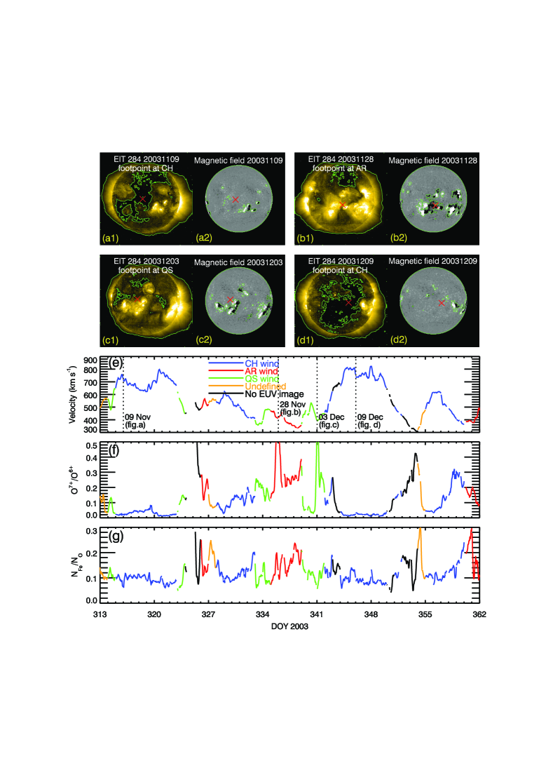
Figure 1:   Top panel (a–d) illustrates the classification scheme of the solar wind. Figures a1, b1, c1 and d1 present the EIT 284 Å images, while a2, b2, c2, d2 give the corresponding photospheric magnetograms, with green contours outlining the CHs and MCA boundaries, respectively. The footpoints of the solar wind are denoted by red crosses. The solar wind detected by ACE is classified as CH wind (a1, a2 and d1, d2), AR wind (b1, b2) and QS wind (c1, c2). Bottom panels: Solar wind parameters for days 313–361 of 2003. Panel (e)–(g) show the speeds, O⁷⁺/O⁶⁺, and $N_{Fe}/N_{O}$Ṫhe wind streams from CHs, ARs, and the QS are represented by blue, red, and green lines, respectively. The orange lines denote the undefined wind type, and the black lines represent the days during which there is no EUV image taken by EIT. The vertical lines represent the solar wind flows whose footpoint is shown in figure (a)–(d), respectively.

Table 1: The contribution of different source regions to FSW and SSW   determined from the ACE measurements during a given solar cycle phase.

		FSW			SSW
	CH	AR	QS	CH	AR	QS
ALL	39.3%	25.2%	35.5%	13.4%	42.9%	43.7%
MAX	34.1%	40.3%	25.6%	12.1%	58.8%	29.1%
DEC	48.2%	24.0%	27.8%	16.1%	41.5%	42.3%
MIN	23.2%	12.4%	64.3%	11.2%	15.9%	72.9%

Table 2: The proportion of FSW and SSW   determined from the ACE measurements for a given source region during different solar cycle phases.

	ALL		MAX		DEC		MIN
	FSW	SSW	FSW	SSW	FSW	SSW	FSW	SSW
CHs	59.3%	40.7%	39.5%	60.5%	64.3%	35.7%	57.8%	42.2%
ARs	22.6%	77.4%	13.7%	86.3%	25.8%	74.2%	34.0%	66.0%
QS	28.8%	71.2%	17.0%	83.0%	28.4%	71.6%	36.8%	63.2%

As the magnetic field configurations and plasma properties are significantly different for the different types of source regions, we investigate here whether there also exist differences between the three sources of solar wind. In Figure 2, we show the   normalized (to the maximum for each wind type) distributions of the solar wind speed and the O⁷⁺/O⁶⁺ and $N_{Fe}/N_{O}$ ratios for the solar wind as a whole (in order to compare with earlier studies) and the different source regions, i.e. AR, QS and CH. As these parameters are expected to change with the solar activity (Lepri et al., 2013; Fu et al., 2015), the results are shown for three different phases of solar cycle 23. From Figure 2 (a1) we note that as expected the average speed of the CH wind is higher than the AR and QS wind. Further, we estimated the contribution of each of the source regions to the fast and the slow solar wind (Table 1). If the whole cycle is considered as one, the CHs (39.3%) have just a $\sim$4% higher contribution to the FSW than the QS (35.5%), with ARs having the smallest input of 25.2%. For a given solar cycle phase, however, the true contribution of each type of solar wind becomes more evident. During the maximum phase of the solar cycle, the ARs are the dominant FSW source at 40.3% followed by the CHs at 34.1% and the QS at 25.6%. At the time of the decline phase the CHs are prevailing at 48.2% and the rest of the FSW input comes almost equally from the QS (24.0%) and ARs (27.8%). The most dominant during the minimum is the QS at 64.3%. With regard to the SSW, if all the whole cycle is examined, the QS (43.7%) and ARs (42.9%) have an almost equal contribution. At the maximum ARs are the main source of SSW at 58.8%, while in the decline phase again the AR and QS have almost the same contribution of $\sim$42%. The predominant source of the SSW during the minimum of the solar activity is the QS at 72.9%.

The fractional contribution of each wind for a given source region is shown in Table  2. Again if all solar cycle phases together are studied, then CHs produce $\sim$60% FSW ($\sim$40% SSW), ARs $\sim$77% SSW of their total solar wind input, while $\sim$29% of the total QS contribution goes into the FSW. More interesting is, however, how the fractions change during the different phases of the solar cycle activity. During the maximum CH SSW rises to $\sim$60%, while the solar main contribution of ARs and QS (of more than $\sim$80%) is to the SSW. In the decline phase the CH produces more FSW ($\sim$64%) than SSW ($\sim$36%). Again the ARs and QS are predominantly contributing to the SSW at a bit more than $\sim$70% of their total wind contribution. During the minimum the CH FSW contribution decreases slightly to $\sim$58% while the emission of SSW grows to $\sim$42%. In the minimum the FSW contribution of the ARs and QS goes further up to  34% and  37%, respectively, while their SSW contribution decrease.  It is important to point out that the above results only reflect the wind detected by ACE which lies in the ecliptic plane. Also we have to note that the heliospheric structures (such as neutral line and heliospheric current sheet) which may influence the statistical results were not removed during the investigated years. Usually, those structures are associated with the boundaries between different source regions of the solar wind (Neugebauer et al., 2002).

Case and statistical studies have already shown that CHs are sources of both the fast and slow wind (Neugebauer et al., 2002; Ko et al., 2014). Woo & Habbal (2000) compared the flow speed derived from Doppler dimming and density observations by UVCS/SoHO (UltraViolet Coronagraph Spectrometer) and suggested that the QS regions are an additional source of the fast solar wind, thus questioning the   traditional belief that the fast solar wind originates only from CHs.   There are many small regions (size of several arcsec across) in a typical QS region that are similar in brightness to CH regions as observed in, for instance, coronal spectral lines Ne viii (T_max $\sim$ 6$\times$10⁵ K) and Mg x (T_max $\sim$ 10⁶ K) (from SUMER), as well as EIT and TRACE coronal solar-disk images. Thus, Feldman et al. (2005) speculated that those dark QS regions may be the source regions of the fast solar wind suggested by Woo & Habbal (2000). In the present study, the solar wind is classified by source regions which differs from classifications that are based on solar wind parameters (such as solar wind speed and charge state O⁷⁺/O⁶⁺) (Zhao et al., 2009; Landi et al., 2012). Bearing the uncertainties of our solar-wind classification scheme as discussed in Fu et al. (2015) (such as the reliability of the PFSS model and the simple ballistic treatment in the mapping procedure), our results demonstrate the complexity of the fast and slow solar wind origin.

A significant feature for the CH wind speeds are their two peak distributions for all three solar activity phases. We   suggest that the fast and slow distribution peaks come from the CH center and the boundary regions that include both CH open and QS/AR close magnetic fields, respectively. For instance, as shown in the wind-source identification example in Figure 1, the solar wind streams coming from CH core regions are faster, while the CH boundary streams are slower. Similar results are shown by Neugebauer et al. (2002, see Figure 11 in their paper) and Ko et al. (2014, Figure 1 in their paper). Several studies have suggested that structures like coronal bright points and plumes which are located in CH boundary regions may also be sources of the SSW (e.g., Madjarska et al., 2004; Subramanian et al., 2010; Madjarska et al., 2012; Fu et al., 2014; Karpen et al., 2016). This can be interpreted by both the WTD and RLO models. In the WTD models, it means that the super radial expansion and curvature degree of the open magnetic-field lines are smaller and lower at the center of CHs compared to CH boundary regions. RLO models suggest that loops that reconnect with open magnetic-field lines have lower temperature at CH central regions than loops located in the boundary regions. The two peak distribution of solar wind speeds may, therefore, reflect either the super radial expansion and the curvature degree of the open magnetic-field lines, or loop temperature.

As shown in Figure 2, (b1) the CH solar-wind speed distribution has a stronger peak at $\sim$400 km s^-1, and a second weaker peak at $\sim$600 km s^-1 during the solar maximum. During the decline and minimum phases, the second peak at $\sim$600 km s^-1 is stronger than the peak at lower speeds.   The two-peak distribution variation of the CH wind may be related to the different average areas and physical properties (such as magnetic field strength) of CHs during different solar activity phases (Wang, 2009). Another possible explanation is the difference of the heliospheric structure during the different solar cycle phases. During solar maximum, ACE may encounter a longer period of neutral line or heliospheric current sheet which usually corresponds to the SSW, thus the slow wind peak is higher. The faster peak at $\sim$600 km s^-1 is stronger because there are more equatorial CHs during the decline phase (Wang, 2009).

As it can be seen from the middle and bottom rows in Figure 2, in all three phases of the solar cycle discussed here the average values of O⁷⁺/O⁶⁺ and $N_{Fe}/N_{O}$ are the highest for the AR wind, the lowest for the CH wind with the QS wind in between. Consistent with Kilpua et al. (2016), our study demonstrates that the distributions of the speed, O⁷⁺/O⁶⁺, and $N_{Fe}/N_{O}$ ratios for the different types of solar wind have a large overlap, and therefore, it is hard to distinguish the source regions only by those wind parameters. The other characteristics for the parameters of O⁷⁺/O⁶⁺ and $N_{Fe}/N_{O}$ ratio will be discussed in Section 3.2 and 3.3

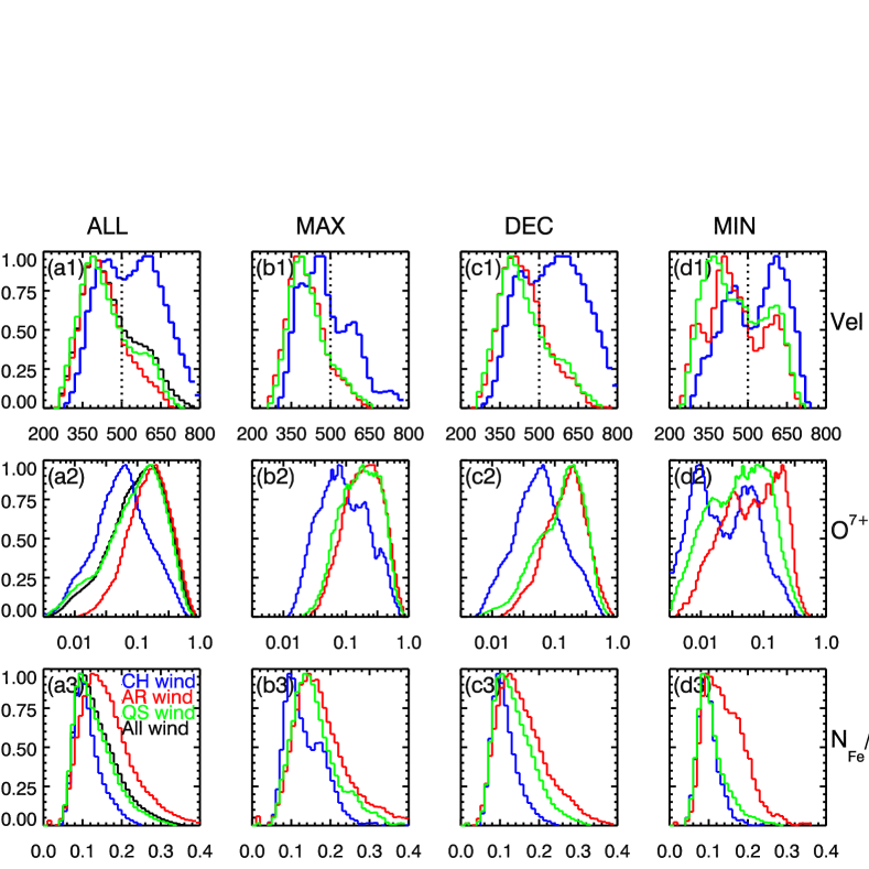
Figure 2: The  normalized distributions of the solar wind parameters. The rows represent the parameters speed, O⁷⁺/O⁶⁺, and $N_{Fe}/N_{O}$  while the first column is the solar wind as a whole, and the second (third, and fourth) column corresponds to the solar maximum (declining, and minimum) phase. Blue, red, and green represents the CH, AR, and QS wind separately. Although there are some differences in parameter distributions for different types of solar wind, it has a big over-lap. The significant characteristic is a bimodal speed distribution for CH wind in all three solar phases.

3.2 Distributions in the space of speed vs O⁷⁺/O⁶⁺

Figure 3 shows the scatter plot of O⁷⁺/O⁶⁺ versus the solar wind speed for the different source regions, i.e. CH, AR, and QS. For the purpose of being comparable to previous studies, we show in column 1 of Figure 3 the relation between O⁷⁺/O⁶⁺ and the solar wind speeds for all three regions summed together. The distributions for each individual source regions are shown in column 2, 3 and 4 of Figure 3. The anti-correlation of the solar wind speed and O⁷⁺/O⁶⁺ remains valid for all three types of solar wind. In the left column of Figure 3, the linear fit of the distributions for the different source regions of solar wind are overplotted, showing that slopes and intercepts are the same for the different solar-wind source regions.   Quantitatively, the slops are $-0.0027,-0.0028$ and $-0.0028$ for CH, AR and QS wind, respectively, during solar maximum, and $-0.0026,-0.0025,-0.0030$ at the decline phase, and $-0.0038,-0.0035,-0.0034$ during the solar minimum. The absolute values of the slops for a certain type of solar wind are almost constant during the solar maximum and decline phases and larger during the solar minimum.

The anti-correlation between solar wind speed and O⁷⁺/O⁶⁺ was first reported by observations from the International Sun-Earth Explorer 3 (ISEE 3) and Ulysses (Ogilvie et al., 1989; Geiss et al., 1995). Gloeckler et al. (2003) suggested that this observational fact supports the notion that the mechanism suggested by the RLO models is the main physical process for heating and acceleration of the nascent solar wind. Our statistical study shows that the anti-correlation between solar wind speeds and O⁷⁺/O⁶⁺ is not only present for the CH wind (Ko et al., 2014) but is also valid for the AR and QS wind. This suggests that the mechanisms which account for the anti-correlation between the solar wind speeds and O⁷⁺/O⁶⁺ ratio are the same in CH, QS, and AR wind. Relating to the RLO models, this means that the correlation between loop size and loop temperature is similar in all three types of regions. With regard to the WTD models, this suggests that the super radial expansion and curvature degree of the open magnetic filed lines is proportional to the source region temperature.   The anti-correlation between the solar wind speed and O⁷⁺/O⁶⁺ can also be explained by a scaling law, in which a higher coronal electron temperature leads to more energy lost from radiation for SSW, and vice versa as suggested by Schwadron & McComas (2003), Schwadron et al. (2014), and Schwadron et al. (2011). This scaling law is required for all magnetically driven solar wind models. Considering that the physical parameters and magnetic field configurations for a certain type of region (CH, AR and QS) have a large range, our statistical results for the different types of solar wind provide a test for this scaling law. Our results demonstrate that the relationship for solar wind speed and O⁷⁺/O⁶⁺ is valid and is almost the same for different types of solar wind, which means the scaling law is valid in all three types of solar wind.

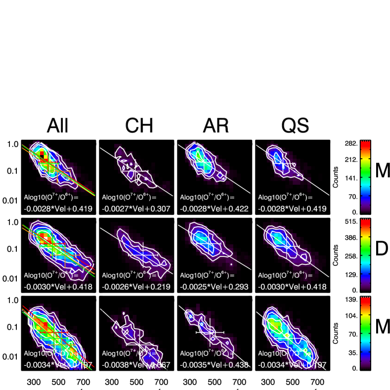
Figure 3: The distribution of solar wind originating in CH, AR, and QS regions in the speed–O⁷⁺/O⁶⁺ space. The first to fourth column represents the wind as a whole, and from CH, AR, and QS regions, respectively, while the top (middle, bottom) panel corresponds to the solar maximum (declining, minimum) phase. In the left column, the white line represents the linear fitting result for the solar wind as a whole, and orange (red, green) represents the wind coming from CH (AR, QS) regions. The slopes and intercepts are given in the bottom of each figure. The error bars represent the standard deviations of speed and O⁷⁺/O⁶⁺ratio. The counts mean the number of hourly solar wind units detected by the ACE satellite.

3.3 Distributions in the space of speed vs $N_{Fe}/N_{O}$ 

Figure 4 presents the scatter plot of the solar wind speed versus $N_{Fe}/N_{O}$  again for all three regions together in column 1, and for the individual source regions in columns 2, 3, and 4. The distribution for all three regions together is similar to earlier studies (e.g. Abbo et al., 2016, and the references therein). There are four important features concerning the relation between $N_{Fe}/N_{O}$ and the solar wind speeds. First, the average value of $N_{Fe}/N_{O}$ is the highest in the AR wind, and the lowest for the CH wind. Second, the $N_{Fe}/N_{O}$ range (0.06–0.40, FIP bias range 1–7) for the AR wind is wider than for the CH wind (0.06–0.20, FIP bias range 1–3). Third, similar to the wind as a whole, the $N_{Fe}/N_{O}$ ranges and their average values all decrease with the increasing solar wind speed in the different types of solar wind. Fourth, the minimum value of $N_{Fe}/N_{O}$ is similar ($\sim$0.06, FIP bias $\sim$1) for all source regions and it does not change with the speed of the solar wind.

The remote measurements in the solar corona given by Widing & Feldman (2001), Brooks & Warren (2011), and Baker et al. (2013) show that the FIP bias is higher in AR regions (dominated by loops) than in CHs. The FIP bias in CHs is between 1 and 1.5 (Feldman et al., 2005), while in ARs it can reach values larger than 4 in the case of older ARs (Widing & Feldman, 2001). The remote measurements of the solar corona also show that the variation of FIP bias in ARs is larger than in CHs (McKenzie & Feldman, 1992; Widing & Feldman, 2001). Our results demonstrate that the $N_{Fe}/N_{O}$ ranges and their average value are higher in the AR wind. This means that the plasma stored in closed loops can escape into interplanetary space, and that this mass supply scenario is consistent with the RLO models.

The differences in $N_{Fe}/N_{O}$ ranges and their average values between different source regions of solar wind can also be explained qualitatively by the RLO models.   Feldman et al. (2005) reviewed the morphological features in the upper atmosphere. They showed that the small loops (10–20 arcsecs) are cooler (30 000 K to 0.7 MK) and have shorter lifetime (100 to 500 s) in QS and CH regions. There are also larger loops (tens to hundreds of arcsecs) which have higher temperature (1.2–1.6 MK) and longer lifetime (1–2 days) in QS regions. By reconstructing the magnetic field with the help of a potential magnetic field model, Wiegelmann & Solanki (2004) suggest that the loops in CHs are on average flatter and shorter than in the QS. The range of loop sizes and temperatures are wider in AR regions including small (10–20 arcsecs) cool ($<$0.1 MK) loops (Huang et al., 2015), as well cool (0.1 MK – 1 MK), warm (1–2M K) and hot hot ($>$ 2 MK) loops with lengths ranging from a few tens to a few hundreds of arcsecs (e.g. Landi & Landini, 2004; Aschwanden et al., 2008, Xie et al. ApJ (submitted)). The above results mean that the ranges of temperatures and loop sizes are wider in AR regions than in CHs. Although this relation is not strictly proportional, the lifetime of loops is connected to these parameters. Widing & Feldman (2001) studied the FIP bias of four emerging active regions and found that the FIP bias increases progressively after the emergence. They concluded that the low FIP elements enrichment relates to the age of coronal loops. The AR wind may both come from new loops (with low FIP bias) and old loops (with higher FIP bias). Therefore, the $N_{Fe}/N_{O}$ range and its average value in the AR wind is wider (higher) than in the CH wind.

The fact that $N_{Fe}/N_{O}$ range and average value decrease with the increasing solar wind speed in all three types of solar wind (see Figure 4) can also be explained qualitatively by the RLO models. Fisk (2003) showed that the speed of the solar wind is inverse to the loop temperatures. For the fast wind, the loops in the source regions are cooler and their life time is shorter. Thus, their FIP bias is lower and its distribution range is narrower. In contrast, the slow wind is at the other extreme. There are two possible interpretations for the fact that the minimum value of $N_{Fe}/N_{O}$ is similar ($\sim$0.06, FIP bias $\sim$1) for all source regions and it does not change with speed of the solar wind. First, in the RLO models, some of the new born loops (size may be large or small) reconnect with the open field lines producing solar wind with lower $N_{Fe}/N_{O}$ (wind speed is slow or fast).   Second, based on the WTD models the solar wind escapes directly along the open magnetic field lines and the FIP fractionation is restricted to the top of the chromosphere based on a model in which the FIP fractionation is caused by ponderomotive force (Laming, 2004, 2012). Thus, the FIP bias is lower ($\sim$1–2) in open filed lines compared with that in the closed loops ($\sim$2–7, please see Table 3 and 4 in Laming (2015)). In all three types of regions, the solar wind which escapes from open magnetic filed lines directly has lower FIP bias, regardless of whether the speed is slow or fast.

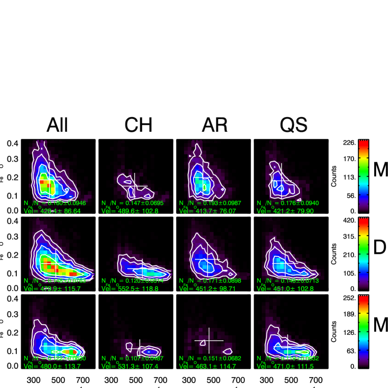
Figure 4: Similar to Figure 3, but for the distribution of solar wind in the speed–$N_{Fe}/N_{O}$ space. The overall behavior is similar for different source regions of solar wind. The $N_{Fe}/N_{O}$ range in AR wind is wider than in CH wind. The minimum of $N_{Fe}/N_{O}$ does not change with speed, and it is similar for different source regions of solar wind.

4 Summary and concluding remarks

The main purpose of this work was to examine the statistical properties of the solar wind originating from different solar regions, i.e. CHs, ARs, and QS. The solar wind speeds, O⁷⁺/O⁶⁺, and $N_{Fe}/N_{O}$ were analyzed for different solar cycle phases (maximum, decline, and minimum). Our main results can be summarized as follows:

1. We found in the present study that the proportions of FSW and SSW are 59.3% and 40.7% for CH regions. Fast solar wind is also found to emanate from AR and the QS, and the proportion of the FSW from AR and QS with respect to their total solar wind input are 13.7% and 17.0%, 25.8% and 28.4%, 34.0% and 36.8%, during the solar maximum, decline, and minimum phases, respectively. The distributions of speed, O⁷⁺/O⁶⁺, and $N_{Fe}/N_{O}$ ratio for the different source regions of solar wind have large overlaps indicating that it is hard to distinguish the source regions only by those wind parameters.

2. We found that the speed distribution of the CH wind is bimodal in all three solar activity phases. The peak of the fast wind from CHs for the period of time studied here is found to be at $\sim$ 600 km s^-1 and the slow wind peak is at $\sim$ 400 km s^-1. The fast and slow wind components possibly come from the center and boundary regions of CHs, respectively.

3. This study demonstrates that the anti-correlation between the speed and O⁷⁺/O⁶⁺ ratio remains valid in all three types of solar wind and during the three studied solar cycle activity phases.

4. We identify four features of the distribution of $N_{Fe}/N_{O}$ in the different solar wind types. The average value of $N_{Fe}/N_{O}$ is highest in the AR wind, and lowest for the CH wind. The average values and ranges of $N_{Fe}/N_{O}$ all decrease with the solar wind speed. The $N_{Fe}/N_{O}$ range in the AR wind is larger (0.06–0.40) than in CH wind (0.06–0.20). The minimum value of $N_{Fe}/N_{O}$ ($\sim$ 0.06) does not change with the variation of speed, and it is similar for all source regions.

The statistical results indicate that the solar wind streams that come from different source regions are subject to similar constraints. This suggests that the heating and acceleration mechanisms of the nascent solar wind in coronal holes, active regions, and quiet Sun have great similarities. The two-peak distribution of the CH wind and the anti-correlation between the speed and O⁷⁺/O⁶⁺ in all three types of solar wind can be explained qualitatively by both the WTD and RLO models, whereas the distribution features of $N_{Fe}/N_{O}$ in different source regions of solar wind can be explained more reasonably by the RLO models.

References

- Abbo et al. (2016) Abbo, L., Ofman, L., Antiochos, S. K., et al. 2016, Space Sci. Rev., 201, 55
- Antiochos et al. (2012) Antiochos, S. K., Linker, J. A., Lionello, R., et al. 2012, Space Sci. Rev., 172, 169
- Aschwanden et al. (2008) Aschwanden, M. J., Nitta, N. V., Wuelser, J.-P., & Lemen, J. R. 2008, ApJ, 680, 1477
- Asplund et al. (2009) Asplund, M., Grevesse, N., Sauval, A. J., & Scott, P. 2009, ARA&A, 47, 481
- Baker et al. (2013) Baker, D., Brooks, D. H., Démoulin, P., et al. 2013, ApJ, 778, 69
- Brooks & Warren (2011) Brooks, D. H., & Warren, H. P. 2011, ApJ, 727, L13
- Buergi & Geiss (1986) Buergi, A., & Geiss, J. 1986, Sol. Phys., 103, 347
- Cranmer (2009) Cranmer, S. R. 2009, Living Reviews in Solar Physics, 6, 3
- Cranmer et al. (2007) Cranmer, S. R., van Ballegooijen, A. A., & Edgar, R. J. 2007, ApJS, 171, 520
- Culhane et al. (2014) Culhane, J. L., Brooks, D. H., van Driel-Gesztelyi, L., et al. 2014, Sol. Phys., 289, 3799
- Delaboudinière et al. (1995) Delaboudinière, J.-P., Artzner, G. E., Brunaud, J., et al. 1995, Sol. Phys., 162, 291
- Domingo et al. (1995) Domingo, V., Fleck, B., & Poland, A. I. 1995, Sol. Phys., 162, 1
- Feldman et al. (2005) Feldman, U., Landi, E., & Schwadron, N. A. 2005, Journal of Geophysical Research (Space Physics), 110, A07109
- Fisk (2003) Fisk, L. A. 2003, Journal of Geophysical Research (Space Physics), 108, 1157
- Fisk et al. (1999) Fisk, L. A., Schwadron, N. A., & Zurbuchen, T. H. 1999, J. Geophys. Res., 104, 19765
- Fisk & Zurbuchen (2006) Fisk, L. A., & Zurbuchen, T. H. 2006, Journal of Geophysical Research (Space Physics), 111, A09115
- Fu et al. (2015) Fu, H., Li, B., Li, X., et al. 2015, Sol. Phys., 290, 1399
- Fu et al. (2014) Fu, H., Xia, L., Li, B., et al. 2014, ApJ, 794, 109
- Geiss et al. (1995) Geiss, J., Gloeckler, G., & von Steiger, R. 1995, Space Sci. Rev., 72, 49
- Gloeckler et al. (2003) Gloeckler, G., Zurbuchen, T. H., & Geiss, J. 2003, Journal of Geophysical Research (Space Physics), 108, 1158
- Gloeckler et al. (1998) Gloeckler, G., Cain, J., Ipavich, F. M., et al. 1998, Space Sci. Rev., 86, 497
- Gosling & Pizzo (1999) Gosling, J. T., & Pizzo, V. J. 1999, Space Sci. Rev., 89, 21
- Hollweg (1986) Hollweg, J. V. 1986, J. Geophys. Res., 91, 4111
- Huang et al. (2015) Huang, Z., Xia, L., Li, B., & Madjarska, M. S. 2015, ApJ, 810, 46
- Karpen et al. (2016) Karpen, J. T., DeVore, C. R., Antiochos, S. K., & Pariat, E. 2016, ArXiv e-prints, arXiv:1606.09201
- Kilpua et al. (2016) Kilpua, E. K. J., Madjarska, M. S., Karna, N., et al. 2016, Sol. Phys., 291, 2441
- Ko et al. (2014) Ko, Y.-K., Muglach, K., Wang, Y.-M., Young, P. R., & Lepri, S. T. 2014, ApJ, 787, 121
- Kojima et al. (1999) Kojima, M., Fujiki, K., Ohmi, T., et al. 1999, J. Geophys. Res., 104, 16993
- Krieger et al. (1973) Krieger, A. S., Timothy, A. F., & Roelof, E. C. 1973, Sol. Phys., 29, 505
- Krista & Gallagher (2009) Krista, L. D., & Gallagher, P. T. 2009, Sol. Phys., 256, 87
- Laming (2004) Laming, J. M. 2004, ApJ, 614, 1063
- Laming (2012) —. 2012, ApJ, 744, 115
- Laming (2015) —. 2015, Living Reviews in Solar Physics, 12, 2
- Landi et al. (2012) Landi, E., Alexander, R. L., Gruesbeck, J. R., et al. 2012, ApJ, 744, 100
- Landi & Landini (2004) Landi, E., & Landini, M. 2004, ApJ, 608, 1133
- Landi et al. (2014) Landi, E., Oran, R., Lepri, S. T., et al. 2014, ApJ, 790, 111
- Lepri et al. (2013) Lepri, S. T., Landi, E., & Zurbuchen, T. H. 2013, ApJ, 768, 94
- Li et al. (2011) Li, B., Xia, L. D., & Chen, Y. 2011, A&A, 529, A148
- Luhmann et al. (2002) Luhmann, J. G., Li, Y., Arge, C. N., Gazis, P. R., & Ulrich, R. 2002, Journal of Geophysical Research (Space Physics), 107, 1154
- Madjarska et al. (2004) Madjarska, M. S., Doyle, J. G., & van Driel-Gesztelyi, L. 2004, ApJ, 603, L57
- Madjarska et al. (2012) Madjarska, M. S., Huang, Z., Doyle, J. G., & Subramanian, S. 2012, A&A, 545, A67
- McKenzie & Feldman (1992) McKenzie, D. L., & Feldman, U. 1992, ApJ, 389, 764
- Neugebauer et al. (2002) Neugebauer, M., Liewer, P. C., Smith, E. J., Skoug, R. M., & Zurbuchen, T. H. 2002, Journal of Geophysical Research (Space Physics), 107, 1488
- Neugebauer et al. (1998) Neugebauer, M., Forsyth, R. J., Galvin, A. B., et al. 1998, J. Geophys. Res., 103, 14587
- Ogilvie et al. (1989) Ogilvie, K. W., Coplan, M. A., Bochsler, P., & Geiss, J. 1989, Sol. Phys., 124, 167
- Owocki et al. (1983) Owocki, S. P., Holzer, T. E., & Hundhausen, A. J. 1983, ApJ, 275, 354
- Richardson & Cane (2004) Richardson, I. G., & Cane, H. V. 2004, Journal of Geophysical Research (Space Physics), 109, A09104
- Sakao et al. (2007) Sakao, T., Kano, R., Narukage, N., et al. 2007, Science, 318, 1585
- Scherrer et al. (1995) Scherrer, P. H., Bogart, R. S., Bush, R. I., et al. 1995, Sol. Phys., 162, 129
- Schwadron & McComas (2003) Schwadron, N. A., & McComas, D. J. 2003, ApJ, 599, 1395
- Schwadron et al. (2011) Schwadron, N. A., Smith, C. W., Spence, H. E., et al. 2011, ApJ, 739, 9
- Schwadron et al. (2014) Schwadron, N. A., Goelzer, M. L., Smith, C. W., et al. 2014, Journal of Geophysical Research (Space Physics), 119, 1486
- Schwenn (2006) Schwenn, R. 2006, Space Sci. Rev., 124, 51
- Stone et al. (1998) Stone, E. C., Frandsen, A. M., Mewaldt, R. A., et al. 1998, Space Sci. Rev., 86, 1
- Subramanian et al. (2010) Subramanian, S., Madjarska, M. S., & Doyle, J. G. 2010, A&A, 516, A50
- Verdini et al. (2009) Verdini, A., Velli, M., & Buchlin, E. 2009, Earth Moon and Planets, 104, 121
- von Steiger et al. (2000) von Steiger, R., Schwadron, N. A., Fisk, L. A., et al. 2000, J. Geophys. Res., 105, 27217
- Wang (2009) Wang, Y.-M. 2009, Space Sci. Rev., 144, 383
- Wang et al. (2009) Wang, Y.-M., Ko, Y.-K., & Grappin, R. 2009, ApJ, 691, 760
- Wang & Sheeley (1990) Wang, Y.-M., & Sheeley, Jr., N. R. 1990, ApJ, 355, 726
- Wang & Sheeley (1991) —. 1991, ApJ, 372, L45
- Wang & Sheeley (2003) —. 2003, ApJ, 587, 818
- Widing & Feldman (2001) Widing, K. G., & Feldman, U. 2001, ApJ, 555, 426
- Wiegelmann & Solanki (2004) Wiegelmann, T., & Solanki, S. K. 2004, Sol. Phys., 225, 227
- Woo & Habbal (2000) Woo, R., & Habbal, S. R. 2000, J. Geophys. Res., 105, 12667
- Woo et al. (2004) Woo, R., Habbal, S. R., & Feldman, U. 2004, ApJ, 612, 1171
- Zhao et al. (2009) Zhao, L., Zurbuchen, T. H., & Fisk, L. A. 2009, Geophys. Res. Lett., 36, L14104
- Zirker (1977) Zirker, J. B. 1977, Reviews of Geophysics and Space Physics, 15, 257