Bistable director alignments of nematic liquid crystals confined in frustrated substrates

Abstract

We studied in-plane bistable alignments of nematic liquid crystals confined by two frustrated surfaces by means of Monte Carlo simulations of the Lebwohl-Lasher spin model. The surfaces are prepared with orientational checkerboard patterns, on which the director field is locally anchored to be planar yet orthogonal between the neighboring blocks. We found the director field in the bulk tends to be aligned along the diagonal axes of the checkerboard pattern, as reported experimentally [J.-H. Kim et al., Appl. Phys. Lett. 78, 3055 (2001)]. The energy barrier between the two stable orientations is increased, when the system is brought to the isotropic-nematic transition temperature. Based on an elastic theory, we found that the bistability is attributed to the spatial modulation of the director field near the frustrated surfaces. As the block size is increased and/or the elastic modulus is reduced, the degree of the director inhomogeneity is increased, enlarging the energy barrier. We also found that the switching rate between the stable states is decreased when the block size is comparable to the cell thickness.

I Introduction

Liquid crystals have been utilized in many applications. In particular, they are widely used in optical devices such as flat panel displays Rasing and Muševič (2004); Chen (2011). Because of the softness of the liquid crystal, its director field is deformed by relatively weak external fields de Gennes and Prost (1995). To sustain the deformed state, the external field has to be constantly applied to the liquid crystal substance. In order to reduce power consumption, a variety of liquid crystal systems showing multistable director configurations or storage effects have been developed Berreman and Heffner (1981); Clark and Lagerwall (1980); Davidson and Mottram (2002); Cheng et al. (1982); Boyd et al. (1980); Scheffer and Nehring (1984); Parry-Jones et al. (2003); Gwag et al. (2007); Monkade et al. (1988); Barberi et al. (1998); Jägemalm et al. (1998); Dozov et al. (1997); Kim et al. (2001, 2002a, 2003); Yu and Kwok (2004); Tsakonas et al. (2007); Araki et al. (2011, 2013); Lohr et al. (2014). In such systems, a pulsed external field can induce permanent changes of the director configurations. Liquid crystals of lower symmetries, such as cholesteric, ferroelectric and flexoelectric phases, are known to show the storage effects Berreman and Heffner (1981); Clark and Lagerwall (1980); Davidson and Mottram (2002).

A nematic liquid crystal in a simple geometry, e.g. that sandwiched between two parallel plates with homeotropic anchoring, shows a unique stable director configuration if external fields are not imposed. By introducing elastic frustrations, the nematic liquid crystals can have different director configurations of equal or nearly equal elastic energy Boyd et al. (1980); Scheffer and Nehring (1984); Parry-Jones et al. (2003); Araki and Tanaka (2006); Tkakec et al. (2011); Araki et al. (2011, 2013); Araki (2012); Gwag et al. (2007); Lohr et al. (2014). For instance, either of horizontal or vertical director orientation is possibly formed in nematic liquid crystals confined between two flat surfaces of uniformly tilted but oppositely directed anchoring alignments Boyd et al. (1980). Also, it was shown that the nematic liquid crystal confined in porous media shows a memory effect Bellini et al. (2002). The disclination lines of the director field can adopt a large number of trajectories running through the channels of the porous medium Araki et al. (2011, 2013). The prohibition of spontaneous changes of the defect pattern among the possible trajectories leads to the memory effect.

Recent evolutions of micro- and nano-technologies enable us to tailor substrates of inhomogeneous anchoring conditions, the length scale of which can be tuned less than the wavelength of visible light. With them, many types of structured surfaces for the liquid crystals and the resulting director alignments have been reported in the past few decades Scheffer and Nehring (1984); Zhang et al. (2003); Gwag et al. (2007); Lohr et al. (2014); Murray et al. (2014); Tsui et al. (2004); Kim et al. (2002b). For example, a striped surface, in which the homeotropic and planar anchorings appear alternatively, was used to control the polar angle of the director field in the bulk Barbero et al. (1992); Kondrat et al. (2003); Atherton and Sambles (2006).

Kim et al. demonstrated in-plane bistable alignments by using a nano-rubbing technique with an atomic force microscope Kim et al. (2001, 2003). They prepared surfaces of orientational checkerboard patterns. The director field in contact to the surfaces is imposed to be parallel to the surface yet orthogonal between the neighboring domains. They found that the director field far from the surface tends to be aligned along either of the two diagonal axes of the checkerboard pattern. More complicated patterns are also possible to prepare Kim et al. (2002a).

In this paper, we consider the mechanism of the bistable orientations of the nematic liquid crystals confined in two flat surfaces of the checkerboard anchoring patterns. We carried out Monte Carlo simulations of the Lebwohl-Lasher spin model Lebwohl and Lasher (1972) and argued their results with a coarse-grained elastic theory. In particular, the dependences of the stability of the director patterns on the temperature, and the domain size of the checkerboard patterns are studied. Switching dynamics between the stable configurations are also considered.

II Simulation model

We carry out lattice-based Monte Carlo simulations of nematic liquid crystals confined by two parallel plates Lebwohl and Lasher (1972); Chiccoli et al. (1988); Cleaver and Allen (1991); Mondal and Roy (2003); Marguta et al. (2011); Maritan et al. (1994); Priezjev and Pelcovits (2001); Araki et al. (2011); Marguta et al. (2011). The confined space is composed of three-dimensional lattice sites ($L\times L\times H$) and it is denoted by $\mathcal{B}$. Each lattice site $i$ has a unit spin vector $\mbox{\boldmath$u$}_{i}$ ($|\mbox{\boldmath$u$}_{i}|=1$), and the spins are mutually interacting with those at the adjacent sites. At $z=0$ and $z=H+1$, we place substrates, composed of two-dimensional lattices. We put unit vectors $\mbox{\boldmath$d$}_{j}$ on the site $j$ on $\mathcal{S}$, where $\mathcal{S}$ represents the ensemble of the substrate lattice sites. We employ the following Hamiltonian for $\mbox{\boldmath$u$}_{i}$,

$$\mathcal{H} = -\varepsilon\sum_{\langle{i,j}\rangle(\in\mathcal{B})}P_{2}(\mbox{\boldmath$u$}_{i}\cdot\mbox{\boldmath$u$}_{j})$$ (1)

$$-\sum_{i\in\mathcal{B}}P_{2}(\mbox{\boldmath$u$}_{i}\cdot\mbox{\boldmath$e$})-w\sum_{\langle{i,j}\rangle,i\in\mathcal{B},j\in\mathcal{S}}P_{2}(\mbox{\boldmath$u$}_{i}\cdot\mbox{\boldmath$d$}_{j}),$$

where $P_{2}(x)=3(x^{2}-1/3)/2$ is the second-order Legendre function and $\sum_{\langle{i,j}\rangle}$ means the summation over the nearest neighbor site pairs. We have employed the same Hamiltonian to study the nematic liquid crystal confined in porous media Araki et al. (2011).

The first term of the right hand side of Eq. (1) is the Lebwohl-Lasher potential, which describes the isotropic-nematic transition Lebwohl and Lasher (1972); Chiccoli et al. (1988); Cleaver and Allen (1991). In Fig. 1, we plot the temperature dependences of (a) the scalar nematic order parameter $S_{\rm b}$ and (b) the elastic modulus $K$ in a bulk system. The numerical schemes for measuring them are described in Appendix A. We note that a cubic lattice with periodic boundary conditions ($L^{3}=128^{3}$) is used for obtaining $S_{\rm b}$ and $K$ in Fig. 1. As the temperature is increased, both the scalar order parameter and the elastic modulus are decreased and show abrupt drops at the transition temperature $T=T_{\rm IN}$, which is estimated as $k_{\rm B}T_{\rm IN}/\varepsilon\cong 1.12$ Priezjev and Pelcovits (2001).

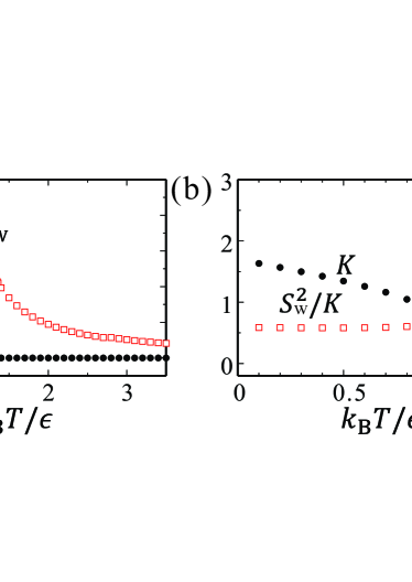
Figure 1: (a) Plots of the scalar nematic order parameter in the bulk $S_{\rm b}$ (black circles) and on the surface $S_{\rm w}$ (red open squares) with respect to the temperature. (b) Plot of the elastic modulus $K$ (black circles) of the nematic phase with $T$. $S_{\rm w}^{2}/K$ is also plotted with red open squares.

The second term of Eq. (1) is the coupling between the spins in $\mathcal{B}$ and an in-plane external field $e$. The last term represents the interactions between the bulk spins and the surface directors, that is, the Rapini-Papoular type anchoring effect Rasing and Muševič (2004); de Gennes and Prost (1995). $w$ is the strength of the anchoring interaction. If $\mbox{\boldmath$d$}_{j}$ is parallel to the substrates and $w>0$, the planar anchoring conditions are imposed to the spins at the $\mathcal{B}$-sites contacting to $\mathcal{S}$. This term not only gives the angle dependence of the anchoring effect in the nematic phase, but also enhances the nematic order near the surface. In Fig. 1(a), we also plot the scalar nematic order parameter on a homogenuous surface of $w=\epsilon$. The definition of $S_{\rm w}$ is described in Appendix A. The nematic order on the surface is larger than that in the bulk $S_{\rm b}$ and is decreased continuously with $T$. Even at and above $T_{\rm IN}$, $S_{\rm w}$ does not vanish to zero. When the temperature is far below $T_{\rm IN}$, on the other hand, it is close to that in the bulk $S_{\rm b}$.

In this study, we prepare two types of anchoring cells. In type I cells, we set hybrid substrates. At the bottom surface $(z=0)$, the preferred direction $\mbox{\boldmath$d$}_{j}$ is heterogeneously patterned like a checkerboard as given by

$$\mbox{\boldmath$d$}_{j}(x,y)=\left\{\begin{array}[]{ll}(0,1,0)&{\rm if}\;([x/D]+[y/D]){\rm\;is\;even}\\ (1,0,0)&{\rm if}\;([x/D]+[y/D]){\rm\;is\;odd}\\ \end{array}\right.,$$ (4)

where $[X]$ stands for the largest integer smaller than a real number $X$. $D$ is the unit block size of the checkerboard pattern. At the top surface $(z=H+1)$, on the other hand, the preferred direction is homogeneously set to $\mbox{\boldmath$d$}_{j}=\mbox{\boldmath$d$}_{\rm t}\equiv(\cos\phi_{\rm t}\sin\theta_{\rm t},\sin\phi_{\rm t}\sin\theta_{\rm t},\cos\theta_{\rm t})$. $\theta_{\rm t}$ and $\phi_{\rm t}$ are the polar and azimuthal angles of the preferred direction at the top surface. In type II cells, both substrates are patterned like the checkerboard, according to Eq. (4).

We perform Monte Carlo simulations with heat bath samplings. A trial rotation of the $i$-th spin is accepted, considering the local configurations of neighboring spins, with the probability $p(\Delta\mathcal{H})=1/(1+e^{\Delta\mathcal{H}/k_{\rm B}T})$, where $\Delta\mathcal{H}$ is the difference of the Hamiltonian between before and after the trial rotation. The physical meaning of the temporal evolution of Monte Carlo simulations is sometimes a matter of debate. However, we note that the method is known to be very powerful and useful for studying glassy systems with slow relaxations, such as a spin glass Ogielski (1985); Araki et al. (2011), the dynamics of which is dominated by activation processes overcoming an energy barrier.

In this study we fix the anchoring strengths at both the surfaces to $w=\varepsilon$, for simplicity. The lateral system size is $L=512$ and the thickness $H$ is changed. For the lateral $x$- and $y$- directions, the periodic boundary conditions are employed.

III Results and discussions

III.1 Bistable alignments

First, we consider nematic liquid crystals confined in cells with the hybrid surfaces (type I). Figure 2(a) plots the energies stored in the cell with respect to the azimuthal anchoring angle $\phi_{\rm t}$. Here the polar anchoring angle is fixed to $\theta_{\rm t}=\pi/2$. The energy per unit area $\mathcal{E}$ is calculated as $\mathcal{E}(\theta_{\rm t},\phi_{\rm t})=\langle{\mathcal{H}(\theta_{\rm t},\phi_{\rm t})}\rangle/L^{2}-\mathcal{E}_{\rm min}$, where $\langle{X}\rangle$ means the spatial average of a variable $X$. $\mathcal{E}_{\rm min}$ is the lowest energy defined as $\mathcal{E}_{\rm min}=\min_{\theta_{\rm t},\phi_{\rm t}}\langle{\mathcal{H}}\rangle/L^{2}$ at each temperature (see below). $\mathcal{E}$ is obtained after $5\times 10^{4}$ Monte Carlo steps (MCS) in the absence of external fields. The cell thickness is $H=16$ and the block size is $D=8$. The temperature is changed.

Figures 2(a) indicates the energy has two minima at $\phi_{\rm t}=\pm\pi/4$, while it is maximized at $\phi_{\rm t}=0$ and $\pm\pi/2$. To see the dependence on the polar angle, we plot $\mathcal{E}$ against $\theta_{\rm t}$ with fixing $\phi_{\rm t}=\pi/4$ in Fig. 2(b). It is shown that $\mathcal{E}$ is minimized at $\theta_{\rm t}=\pi/2$ for $\phi_{\rm t}=\pi/4$. Hence we conclude that the stored energy is globally lowest at $(\theta_{\rm t},\phi_{\rm t})=(\pi/2,\pm\pi/4)$, so that we set $\mathcal{E}_{\rm min}=\langle{\mathcal{H}(\theta_{\rm t}=\pi/2,\phi_{\rm t}=\pi/4)}\rangle/L^{2}$ in Fig. 2. This global minimum indicates that the parallel, yet bistable configurations of the director field are energetically preferred in this cell. This simulated bistability is in accordance with the experimental observations reported by Kim et al. Kim et al. (2001). When a semi-infinite cell is used, the bistable alignments of the director field would be realized. Hereafter, we express these two stable directions with $\hat{\mbox{\boldmath$n$}}_{+}$ and $\hat{\mbox{\boldmath$n$}}_{-}$. That is, $\hat{\mbox{\boldmath$n$}}_{\pm}=(1/\sqrt{2},\pm 1/\sqrt{2},0)$.

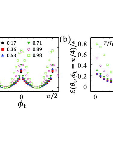
Figure 2: Dependences of the stored energy per unit area with respect to $\phi_{\rm t}$ at $\theta_{\rm t}=\pi/2$ in (a), and to $\theta_{\rm t}$ at $\phi_{\rm t}=\pi/4$ in (b). The liquid crystal is confined in a type I cell of $D=8$ and $H=16$. The temperature is changed.

Figure 2 also indicates the temperature dependencies of the stored energies. When the temperature is much lower than the transition temperature $T_{\rm IN}$, the curves of $\mathcal{E}$ are are rather flat. As the temperature is increased, the dependence becomes more remarkable. Figure 3(a) plots the energy difference between the maximum and minimum of $\mathcal{E}$ for fixed $\theta_{\rm t}=\pi/2$ as functions of $T$. It is defined by the in-plane rotation of $\mbox{\boldmath$d$}_{\rm t}$ as $\Delta\mathcal{E}=\mathcal{E}(\theta_{\rm t}=\pi/2,\phi_{\rm t}=\pi/4)-\mathcal{E}(\pi/2,0)$. We plot them for several block sizes $D$, while the cell thickness is fixed to $H=16$.

In Fig. 3(a), we observe non-monotonic dependences of the energy difference on the temperature. $\Delta\mathcal{E}$ is almost independent of $T$ when $T/T_{\rm IN}<0.6$. In the range of $0.6\lesssim T/T_{\rm IN}<0.9$, it is increased with increasing $T$. When $T/T_{\rm IN}\gtrsim 0.9$, it decreases with $T$ and it almost disappears if $T>T_{\rm IN}$. When $T>T_{\rm IN}$, the system is in the isotropic state, and it does not have the long-range order. Thus, it is reasonable that $\Delta\mathcal{E}$ vanishes when $T>T_{\rm IN}$. When $T<T_{\rm IN}$, on the other hand, it is rather striking that the energy difference shows the non-monotonic dependences on $T$, in spite of that the long-range order and the resultant elasticity are reduced monotonically with increasing $T$ (see Fig. 1).

We plot the energy difference $\Delta\mathcal{E}$ as a function of $D$ in Fig. 3(b), where the temperature is $T/T_{\rm IN}=0.89$. The cell thickness is changed. It is shown that the energy difference $\Delta\mathcal{E}$ is increased proportionally to the block size $D$ when $D$ is small. When the cell thickness is large, on the other hand, the energy difference is almost saturated. The saturated value becomes smaller when the liquid crystal is confined in the thicker cell.

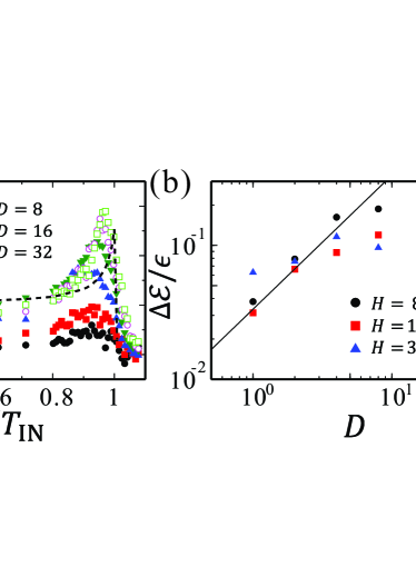
Figure 3: (a) Plot of the energy difference $\Delta\mathcal{E}$ per unit area against the temperature. The cell thickness is $H=8$ (type I) and the block size $D$ is changed. (b) Plot of the energy difference per unit area against the block size. The temperature is $T/T_{\rm IN}=0.89$ and the cell thickness is changed.

In order to clarify the mechanisms of the bistable alignments, we calculate the spatial distribution of the nematic order parameter. In Fig. 4, we show snapshots of $xx$- and $xy$ components of a tensorial order parameter at several planes parallel to the substrates. Using $\mbox{\boldmath$u$}_{i}(t^{\prime})$, the tensorial order parameter $Q_{\mu\nu}$ is calculated by averaging $3/2(u_{\mu}u_{\nu}/2-\delta_{\mu\nu}/3)$ in a certain period $\delta t$ as,

$$Q_{i,\mu\nu}(t)=\frac{1}{\delta t}\sum_{t^{\prime}=t}^{t+\delta t-1}\frac{3}{2}\left\{u_{i,\mu}(t^{\prime})u_{i,\nu}(t^{\prime})-\frac{1}{3}\delta_{\mu\nu}\right\},$$ (5)

where $t^{\prime}$ means the Monte Carlo cycle, and $\mu$ and $\nu$ stand for $x$, $y$ and $z$. In this study, we set $\delta t=10^{2}$, which is chosen so that the system is well thermalized. The block size is $D=8$ in (a) and $D=64$ in (b), and the cell thickness is fixed to $H=8$. The temperature is set to $T/T_{\rm IN}=0.89$. The anchoring direction at the top surface is along $\hat{\mbox{\boldmath$n$}}_{+}$, and we started the simulation with an initial condition, in which the director field is along $\hat{\mbox{\boldmath$n$}}_{+}$, so that the director field is likely to be parallel to the surface and along the azimuthal angle $\phi=\pi/4$ in average.

$Q_{xx}$ near the bottom surface shows the checkerboard pattern as like as that of the imposed anchoring directions $\mbox{\boldmath$d$}_{j}$. $Q_{xy}$ inside the block domains is small and it is enlarged at the edges between the blocks. With departing from the bottom surface, the inhomogeneity is reduced and the director pattern becomes homogeneous along $\hat{\mbox{\boldmath$n$}}_{+}$. The inhomogeneities in $Q_{xx}$ and $Q_{xy}$ are more remarkable for the larger $D$ than those for the smaller $D$.

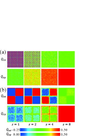
Figure 4: Snapshots of the $xx$- and $xy$ components of the tensorial order parameter $Q_{\mu\nu}$ in the type I cells of the thickness $H=8$. The anchoring direction on the bottom surface ($z=0$) is patterned like the checkerboard, while that on the top surface ($z=9$) is homogeneously along $\hat{\mbox{\boldmath$n$}}_{+}$. The temperature is $T/T_{\rm IN}=0.89$. The block size is $D=8$ in (a) and $D=64$ in (b). Only the snapshots in a small area ($128^{2}$) are shown.

In Fig. 5, we plot the corresponding profiles of the spatial modulations of the order parameter with respect to $z$. The degree of the inhomogeneity of $Q_{\mu\nu}$ is defined by

$$I(z) = \frac{1}{L^{2}S_{\rm b}^{2}}\int dxdy\{Q_{\mu\nu}(x,y,z)-\bar{Q}_{\mu\nu}(z)\}^{2},$$ (6)

where $\bar{Q}_{\mu\nu}(z)$ is the spatial average of $Q_{\mu\nu}$ in the $z$-plane and it is given by

$$\bar{Q}_{\mu\nu}(z) = L^{-2}\int dxdyQ_{\mu\nu}(x,y,z).$$ (7)

$S_{\rm b}$ is the scalar nematic parameter obtained in the bulk [see Fig. 1(a)]. Since $Q_{\mu\nu}\propto S_{\rm b}$ in the bulk, the profiles are scaled by $S^{2}_{\rm b}$ in Eq. (6), in order to see the pure degree of the inhomogeneity of the director field. In Fig. 5(a), we changed the block size $D$ and the temperature is fixed to $T/T_{\rm IN}=0.89$. It is shown that the degree of the inhomogeneity decays with $z$, and it is larger for larger $D$ as shown in Fig. 4. Figure 5(a) also shows that the decaying length is also increased with the block size $D$. Roughly it agrees with $D$. In Fig.5(b), we plot the profiles of $I(z)$ for different temperatures with fixing $D=16$. It is shown that the spatial modulation is increased as the temperature is increased. This is because the nematic phase becomes softer as the temperature is increased (see Fig. 1(b)). When the elastic modulus is small, the director field is distorted by the anchoring surface more largely.

Based on these numerical results, we consider the bistable alignments with a continuum elasticity theory. The details of the continuum theory is described in Appendix B. In our theoretical argument, the spatial modulation of the director field due to the heterogeneous anchoring plays a crucial role in inducing the bistable alignments along the diagonal directions. After some calculations, we obtained an effective anchoring energy for $D\ll H$ as

$$g(\phi_{0})=-\frac{cW^{2}D}{K}\sin^{2}2\phi_{0},$$ (8)

instead of the Rapini-Papoular anchoring energy, $-W\cos^{2}\phi_{0}/2$. Here $\phi_{0}$ is the average azimuthal angle of the director field on the patterned surface. $K$ is the elastic modulus of the director field in the one-constant approximation of the elastic theory, and $W$ represents the anchoring strength in the continuum description. $c$ is a numerical factor, which is estimated as $c\cong 0.085$ when $H/D$ is large. $g(\phi_{0})$ has a fourfold symmetry and is lowered at $\phi_{0}=\pm\pi/4$ and $\pm 3\pi/4$. The resulting energy difference per unit area is given by

$$\Delta\mathcal{E}_{\rm th}=\frac{\pi^{2}K}{32H\{1+K^{2}/(8cW^{2}DH)\}}.$$ (9)

First we discuss the dependence of the energy difference on the block size $D$. Equation (9) indicates that the energy difference behaves as $\Delta\mathcal{E}_{\rm th}\approx\pi^{2}cW^{2}D/(4K)$, which is increased linearly with $D$, when $D$ is sufficiently small. If $D$ is large enough, on the other hand, the energy difference converges to $\Delta\mathcal{E}_{\rm th}\approx\pi^{2}K/(32H)$. The latter energy difference agrees with the deformation energy of the director field, which twists along the $z$ axis by $\pm\pi/4$. It is independent of $D$, but is proportional to $H^{-1}$. The asymptote behaviors for small and large $D$ are consistent with the numerical results shown in Fig. 3(b).

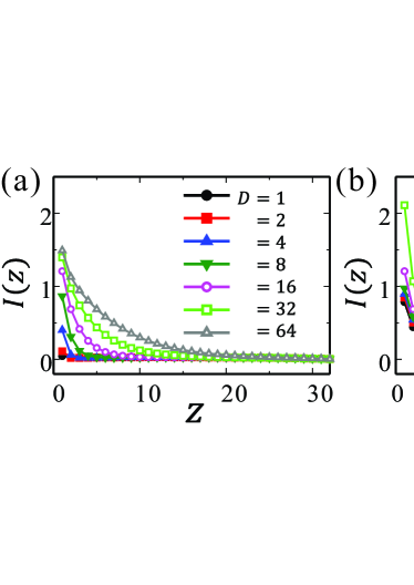
Figure 5: Profiles of the inhomogeneity of the nematic order parameter $I(z)$ along the cell thickness $z$. (a) The cell thickness is $H=32$ (type I) and the temperature is $T/T_{\rm IN}=0.89$. The block size is increased from $D=1$ to $D=64$. (b) The cell thickness is $H=32$ and the block size is fixed to $D=16$. The temperature $T$ is changed.

Next we consider the dependence of $\Delta\mathcal{E}$ on the temperature. Equation (9) also suggests $\Delta\mathcal{E}_{\rm th}$ is proportional to $W^{2}D/K$ when $W^{2}DH/K^{2}$ is small. We have speculated the anchoring strength is simply proportional to the nematic order as $W\propto S_{\rm b}$. If so, the energy difference is expected to be independent of $S_{\rm b}$ as $\Delta\mathcal{E}_{\rm th}\propto W^{2}/K\propto S^{0}_{\rm b}$, since $K$ is roughly proportional to $S_{\rm b}^{2}$. This expectation is inconsistent with the dependence of the numerical results of $\Delta\mathcal{E}$ in Fig. 3(a). A possible candidate mechanism in explaining this discrepancy is that we should use the nematic order on the surface $S_{\rm w}$, instead of $S_{\rm b}$, for estimating $W$. Since $S_{\rm w}$ is dependent on $T$ more weakly than $S_{\rm b}$ near the transition temperature [see Fig. 1(a)], $W^{2}/K$ can be increased with $T$. The curve of $S_{\rm w}^{2}/K$ is drawn in Fig. 1(b). Thus, the director field is more largely deformed near $T_{\rm IN}$ as shown in Fig. 5(b), so that the resulting energy difference shows the increase with $T$.

Also, Fig. 3(a) shows $\Delta\mathcal{E}$ turns to decrease to zero, when we approach to $T_{\rm IN}$ more closely. In the vicinity of $T_{\rm IN}$, $K$ is so small that $W^{2}/K$ becomes large. Then Eq. (9) behaves as $\Delta\mathcal{E}_{\rm th}\propto K/H$. It is decreased to zero as $K$ with approaching to $T_{\rm IN}$. In Fig. 3(a), we draw the theoretical curve of Eq. (9) with taking into account the dependences of $W$ and $K$ on the temperature. Here we assume $W=W_{0}S_{\rm w}$ with $W_{0}$ being a constant. The theoretical curve reproduces the non-monotonic behavior of the energy difference qualitatively. After the plateau of $\Delta\mathcal{E}_{\rm th}$ in the lower temperature region, it is increased with $T$. Then it turns to decrease to zero when the temperature is close to the transition temperature. Here we use $W_{0}=0.3$, which is chosen to adjust the theoretical curve to the numerical result.

III.2 Switching dynamics

Next we confine the nematic liquid crystals in the type II cells, both the surfaces of which are patterned as checkerboard. As indicated by Eq. (8), each checkerboard surface gives rise to the effective anchoring effect with the fourfold symmetry. Hence, the director field is expected to show the in-plane bistable alignments along $\mbox{\boldmath$n$}_{+}$ or $\mbox{\boldmath$n$}_{-}$ also in the type II cells.

Figure 6(a) plots the spatial average of the $xy$ component of $Q_{\mu\nu}$ at equilibrium with respect to the block size. The equilibrium value of $\langle{Q_{xy}}\rangle$ is estimated as $Q_{xy}^{\infty}=\langle{Q_{xy}}\rangle|_{t=5\times 10^{4}}$ in the simulations with no external field. As the initial condition, we employ the director field homogeneously aligned along $\hat{\mbox{\boldmath$n$}}_{+}$, so that $Q_{xy}^{\infty}$ is likely to be positive. In Fig. 6(a), we also draw a line of $3S_{\rm b}/4$, which corresponds to the bulk nematic order when the director field is along $\mbox{\boldmath$n$}_{+}$. It is shown that $Q_{xy}^{\infty}$ is roughly constant and is close to $3S_{\rm b}/4$ for $D\ll H$. It is reasonable since the inhomogeneity of the director field is localized within $D$ from the surfaces. When $D>H$, on the other hand, $Q_{xy}^{\infty}$ is decreased with $D$. When $D\gg H$, the type II cell can be considered as a collection of square domains each carrying the uniform anchoring direction. Thus, the director field tends to be parallel to the local anchoring direction $\mbox{\boldmath$d$}_{j}$, and then, $Q_{xy}$ inside each unit block becomes small locally. Only on the edges of the block domains, the director fields are distorted and adopts either of the distorted states as schematically shown in Fig. 6(b). With scaling $D$ by $H$, the plots of $Q_{xy}^{\infty}$ collapse onto a single curve.

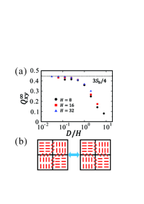
Figure 6: (a) Dependences of the averaged order parameter on the block size. The cell thickness is $H=16$ (type II). The temperature is changed. (b) Schematic pictures of the director field near the mid-plane in the type II cell of $D\gg H$.

Then we consider the switching dynamics of the director field between the two stable alignments with imposing in-plane external fields $e$ in the type II cells. In Fig. 7, we plot the spatial average of the $xy$ component of the order parameter $\langle{Q_{xy}}\rangle$ in the processes of the director switching. The cell size is $H=16$, the block size is $D=16$ and the temperature is $T/T_{\rm IN}=0.89$. At $t=0$, we start the Monte Carlo simulation with the same initial condition, in which the director field is homogeneously aligned along $\hat{\mbox{\boldmath$n$}}_{+}$, in the absence of the external field. As shown in Fig. 7, the nematic order is relaxed to a certain positive value, which agrees with $Q_{xy}^{\infty}$ in Fig. 6(a). From $t_{1}=10^{4}$, we then impose an in-plane external field along $\hat{\mbox{\boldmath$n$}}_{-}$, and turn it off at $t_{2}=2\times 10^{4}$. After the system is thermalized during $t=2\times 10^{4}$ and $t_{3}=3\times 10^{4}$ with no external field, we apply the second external field along $\hat{\mbox{\boldmath$n$}}_{+}$ from $t_{3}=3\times 10^{4}$ until $t_{4}=4\times 10^{4}$. We change the strength of the external field $e$.

When the external field is weak ($e^{2}\leq 0.03$), the averaged orientational order is slightly reduced by the external field, but it recovers the original state after the field is removed. After a strong field ($e^{2}\geq 0.04$) is applied and is removed off, on the other hand, $\langle{Q_{xy}}\rangle$ is relaxed to another steady state value, which is close to $-Q_{xy}^{\infty}$. This new state of the negative $\langle{Q_{xy}}\rangle$ corresponds to the other bistable alignment along $\hat{\mbox{\boldmath$n$}}_{-}$. After the second field along $\hat{\mbox{\boldmath$n$}}_{+}$ is applied, the averaged orientational order $\langle{Q_{xy}}\rangle$ comes back to the positive original value, $+Q_{xy}^{\infty}$.

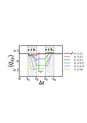
Figure 7: Time sequences of the averaged nematic order along $\hat{\mbox{\boldmath$n$}}_{+}$ in the in-plane switching processes. At $t=0$, the director field is completely aligned along $\mbox{\boldmath$\mbox{\boldmath$n$}$}_{+}$. In time intervals $1\times 10^{4}\leq t<2\times 10^{4}$ and $3\times 10^{4}\leq t<4\times 10^{4}$, the external field is applied along $\hat{\mbox{\boldmath$n$}}_{-}$ and $\hat{\mbox{\boldmath$n$}}_{+}$, respectively. The strength of the external field $e$ is changed. The temperature is $T/T_{\rm IN}=0.89$, and the type II cell of $D=16$ and $H=16$ is employed.

In Fig. 8(a), we show the detailed relaxation behaviors of $\langle{Q_{xy}}\rangle$ in the first switching after $t_{1}$. $\Delta t$ means the elapsed time in the first switching, that is $\Delta t=t-t_{1}$. Here we change the block size $D$, while we fix the external field at $e^{2}=0.03$ and the cell thickness $H=16$ (type II). We note that $\langle{Q_{xy}}\rangle$ at $\Delta t=0$ depends on $D$ as indicated in Fig. 6(a). In Fig. 8(a), it is shown that the switching rate depends also on the block size $D$. Notably, the dependence of the switching behavior is not monotonic against $D$.

In Fig. 8(b), we plot the characteristic switching time $\tau$ with respect to the block size $D$ in the cells of $H=8$, $16$ and $32$. The temperature and the field strength are the same those for Fig. 8(a). The characteristic time $\tau$ is defined such that the average orientational order is equal to zero at $\tau$, $\langle{Q_{xy}}\rangle(\Delta t=\tau)=0$. Figure 8(b) shows the characteristic time is maximized when the block size is comparable to the cell thickness. When $D<H$, the switching process is slowed down as the block size is increased. On the other hand, it is speeded up with $D$ when $D>H$. In Fig. 8(b), it is suggested that the dependence of $\tau$ on $D$ becomes less significant as $H$ is increased.

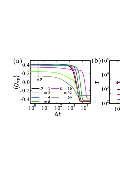
Figure 8: (a) Time sequences of the averaged nematic order parameter $\langle{Q_{xy}}\rangle$ in the switching process. Before $\Delta t=0$, the director field is aligned along $\hat{\mbox{\boldmath$n$}}_{+}$ in average. After $\Delta t=0$, the in-plane external field is applied along $\hat{\mbox{\boldmath$n$}}_{-}$. The temperature is $T/T_{\rm IN}=0.89$ and the cell thickness is $H=16$ (type II). The strength of the external field $e$ is changed. (b) Plots of the characteristic time $\tau$ of the switching process with respect to the block size $D$. $\tau$ is defined as $\langle{Q_{xy}(\Delta t=\tau)}\rangle=0$. The temperature is $T/T_{\rm IN}=0.89$ and the thickness of type II cell is changed.

Figure 9 depicts snapshots of $Q_{xy}(t)$ at the midplane ($z=H/2$) during the first switching process. The parameters are the same as those in Fig. 8(a), so that the pattern evolutions correspond to the curves of $\langle{Q_{xy}}\rangle$ in Fig. 8(a). Figure 9 shows that the switching behavior is slowed down when $D$ is comparable to $H$, in accordance with Fig. 8(b). When $D<H$, the snapshots implies the switching proceeds via nucleation and growth mechanism. From the sea of the positive $Q_{xy}$, where the director is aligned along $\hat{\mbox{\boldmath$n$}}_{+}$, the droplets of the negative $Q_{xy}$ are nucleated. They grow with time and cover the whole area eventually. Under the external field along $\hat{\mbox{\boldmath$n$}}_{-}$, the alignment of the director field along $\hat{\mbox{\boldmath$n$}}_{-}$ is more preferred than that along $\hat{\mbox{\boldmath$n$}}_{+}$. Because of the energy barrier between these bistable alignments, the director field cannot change its orientation to $\hat{\mbox{\boldmath$n$}}_{-}$ smoothly under a weak external field. From Eq. (8), the energy barrier for the local swiching of the director field between the two stable states is given by $\Delta\mathcal{F}=8D^{2}\{g(\phi_{0}=0)-g(\pi/4)\}=8cW^{2}D^{3}/K$, when $D<H$. Thus, the slowing down of the switching process with $D$ is considered to be attributed to the enhancement of the energy barrier. Here we note that a critical field strength for the thermally activated switching cannot be defined unambiguously. Since the new alignment is energetically preferred over the original one even under a weak field, the director configuration will change its orientation if the system is annealed for a sufficiently long period. When the field strength is moderate ($e^{2}\cong 0.035$), the averaged order goes to an intermediate value, neither of $Q_{xy}^{\infty}$ or $-Q_{xy}^{\infty}$ in Fig. 7. Such intermediate values of $\langle{Q_{xy}}\rangle$ reflect large scale inhomogeneities of the bistable alignments (see Fig. 9). At each block, the director field adopts either of the two stable orientations. The pattern of the intermediate $\langle{Q_{xy}}\rangle$ depends not only on the field strength, but also on the annealed time. Under large external fields, on the other hand, the energy barrier between the two states can be easily overcome, so that the switching occurs without arrested at the initial orientation (not shown here).

Regarding the local director field, which adopts either of the two stable orientations ($\hat{\mbox{\boldmath$n$}}_{+}$ and $\hat{\mbox{\boldmath$n$}}_{-}$), as a binarized spin at the corresponding block unit, we found a similarity of the domain growth in our system and that in a two-dimensional Ising model subject to an external magnetic field. If the switching of the director field occurs locally only at each block unit, there is no correlations between the director fields in the adjacent block units. Therefore, the nucleation and growth switching behavior implies the director field at a block unit prefers to be aligned along the same orientation as those at the adjacent block units.

We observed string-like patterns as shown at $\Delta t=4000$ for $D=1$ in Fig. 9. Here we note that they are not disclinations of the director field. They represent domain walls perpendicular to the substrates. In the type II cells, we have not observed any topological defects, although topological defects are sometimes stabilized in the frustrated cell Araki et al. (2011). The string-like patterns remain rather stable transiently. On the other hand, such string-like patterns are not observed in the switching process in the Ising model. This indicates the binarized spin description of the bistable director alignments may be not adequate. Under the external field along $\hat{\mbox{\boldmath$n$}}_{-}$, the director field rotates to the new orientation clockwise or counter-clockwise. New domains, which appear via the clockwise rotations, have some mismatches against those through the counter-clockwise rotations. The resulting boundaries between the incommensurate domains are formed and tend to suppress the coagulations of them more and less, although the corresponding energy barriers are not so large.

When $D>H$, the switching occurs in a different way. The director rotations are localized around the edges of the blocks as indicated in Fig. 6(b). As $D$ is increased, the amount of the director field that reacts to the field is reduced. Although the director fields around the centers of the blocks do not show any switching behaviors before and after the field application, they are distorted to orient slightly toward the field. It is considered that the distortion of the director field inside the blocks effectively reduces the energy barrier against the external field. We have not succeeded in explaining the mechanism of the reduction of the switching time with $D$. When $D>H$, the inhomogeneous director field contains higher Fourier modes of the distortion. The energy barrier for each Fourier mode becomes lower for the higher Fourier modes [see Eq. (18). Thus, such higher Fourier modes are more active against the external field and they would behave as a trigger of the switching process.

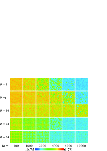
Figure 9: Snapshots of the nematic order parameter $Q_{xy}(x,y)$ at $z=8$ in the type II cell of $H=16$. The director field in yellow regions is along $\hat{\mbox{\boldmath$n$}}_{+}$ and that in blue regions is along $\hat{\mbox{\boldmath$n$}}_{-}$. The temperature is $T/T_{\rm IN}=0.89$ and the block size $D$ is changed.

IV Conclusion

In this article, we studied nematic liquid crystals confined by two parallel checkerboard substrates by means of Monte Carlo simulation of the Lebwohl-Lasher model. As observed experimentally by Kim et al., we found the director field in the bulk shows the bistable alignments, which are along either of the two diagonal axes. We attribute the bistability of the alignments to the spatial modulation of the director field near the substrates. Based on the elastic theory, we derived an effective anchoring energy with the fourfold symmetry (Eq. (8)). Its anchoring strength is expected to behave as $W^{2}D/K$, when the block size $D$ is smaller than the cell thickness. As the temperature is increased to the isotropic-nematic transition temperature, the elastic modulus $K$ of the nematic phase is reduced so that the director field is deformed near the substrates more largely. With this effective anchoring effect, we can explain the non-monotonic dependence of the energy stored in this cell qualitatively.

We also studied the switching dynamics of the director configuration with imposing in-plane external fields. Usually, the switching is considered to be associated with the actual breaking of the anchoring condition. Thus, the energy barrier for the switching is expected to be proportional to $W$ Kim et al. (2001). In this article, we propose another possible mechanism of the switching, in which the anchoring condition is not necessarily broken. Since the energy barrier is increased with the block size, the switching dynamics notably becomes slower when the block size is comparable to the cell thickness.

By solving $\Delta\mathcal{F}=\Delta\epsilon E^{2}/2\times(4D^{2}H)$, we obtain a characteristic strength of the electric field $E$ as $E_{\rm c}\cong\{8cW^{2}D/(\Delta\epsilon KH)\}^{1/2}$, where $\Delta\epsilon$ is the anisotropy of the dielectric constant [see Eq. (11)]. If we apply an in-plane external field larger than $E_{\rm c}$, the switching occurs rather homogeneously without showing the nucleation and growth processes. This characteristic strength is decreased with decreasing $D$, so that the checkerboard pattern of smaller $D$ is preferred to reduce the field strength. With smaller $D$, however, the stability of the two preferred orientations is reduced. If the effective anchoring energy is lower than the thermal energy, the bistable alignment will be destroyed by the thermal fluctuation. In this sense, the block size $D$ should be larger than $D_{\rm c}\approx(Kk_{\rm B}T/8cW^{2})^{1/3}$, where we assumed that the switching occurs locally in each block, that is $\Delta\mathcal{F}\approx k_{\rm B}T$. For a typical nematic liquid crystal with $K=1\,{\rm pN}$ and $W=10^{-5}\,{\rm J/m^{2}}$ at room temperature $T=300\,{\rm K}$, it is estimated as $D_{\rm c}\cong 34\,{\rm nm}$.

In our theoretical argument, we assumed the one-constant approximation of the elastic modulus. However, the director field cannot be described by a single deformation mode in the above cells. The in-plane splay and bend deformations are localized within the layer of $D$ near the surface. On the other hand, the twist deformation is induced by the external field along the cell thickness direction. If the elastic moduli for the three deformation modes are largely different from each other, our theoretical argument would be invalid. We need to improve both the theoretical and numerical schemes to consider such dependences more correctly. Also, we considered only the checkerboard substrates. But, it is interesting and important to design other types of patterned surfaces Kim et al. (2002a) to append more preferred functions, such as faster responses against the external field, to liquid crystal devices. We hope to report a series of such studies in the near future.

Appendix A Estimations of the nematic order and the elastic moduls

In this appendix, we estimate the scalar nematic order parameter and the elastic modulus in Fig. 1 from the Monte Carlo simulations with Eq. (1) Lebwohl and Lasher (1972); Chiccoli et al. (1988); Cleaver and Allen (1991); Mondal and Roy (2003); Marguta et al. (2011); Maritan et al. (1994); Priezjev and Pelcovits (2001); Araki et al. (2011). First we consider the bulk behaviors of nematic liquid crystals, which are described by the Lebwohl-Lasher potential. Here we remove the surface sites $\mathcal{S}$ and employ the periodic boundary conditions for all the axes ($x,y$, and $z$). We use the initial condition along $\mbox{\boldmath$u$}_{i}=(1,0,0)$ and thermalize the system with the heat bath sampling. The simulation box size is $L^{3}$ with $L=128$.

It is well known that this Lebwohl-Lasher spin model describes the first-order transition between isotropic and nematic phases. In Fig. 1, we plot the $xx$ component of the tensorial order parameter after the thermalization ($t\leq 5\times 10^{4}$) as a function of $T$. Since the initial condition is along the $x$ axis, the director field is likely to be aligned along the $x$ axis. We here regard $\langle{Q_{xx}}\rangle$ as the scalar nematic order parameter $S_{\rm b}$. We see an abrupt change of $S_{\rm b}$ around $k_{\rm B}T_{\rm IN}\approx 1.12\epsilon$, which is consistent with previous studies Priezjev and Pelcovits (2001). Above $T_{\rm IN}$, the nematic order almost vanishes, while it is increased with decreasing $T$ when $T<T_{\rm IN}$.

In the nematic phase ($T<T_{\rm IN}$), the director field $n$ can be defined. Because of the thermal noise, the local director field is fluctuating around the average director field, reflecting the elastic modulus. The elastic modulus of the director field is obtained by calculating the scattering function of the tensorial order parameter as Cleaver and Allen (1991),

$$\langle{|\tilde{Q}_{x\mu}(\mbox{\boldmath$q$})|^{2}}\rangle_{T}=\frac{k_{\rm B}T}{A+4L_{Q}\sin^{2}|\mbox{\boldmath$q$}|a/2},$$ (10)

for $\mu=y$ and $z$. $\tilde{Q}_{x\mu}(\mbox{\boldmath$q$})$ is the Fourier component of $Q_{x\mu}$ at a wave vector $q$. $a$ is the lattice constant, and $\langle{\cdots}\rangle_{T}$ means the thermal average. $A$ and $L_{Q}$ are the coefficients appearing in the free energy functional for $Q_{\mu\nu}$.

In the case of $T<T_{\rm IN}$, the scattering function goes to zero for $|\mbox{\boldmath$q$}|a\cong 0$. Then, we obtain the coefficient $L_{Q}$ by fitting $\langle{|\tilde{Q}_{x\mu}|^{2}}\rangle^{-1}_{T}$ with $4(k_{\rm B}T)^{-1}L_{Q}\sin^{2}|\mbox{\boldmath$q$}|a/2$. $L_{Q}$ is proportional to the elastic modulus $K$ of the director field $n$ as $L_{Q}=KS^{2}_{\rm b}$. In Fig. 1(b), the elastic modulus $K$ is plotted with respect to $T$. It is decreased with increasing $T$, if $T>T_{\rm IN}$. This indicates the softening of the nematic phase near the transition temperature.

Next we consider the effect of the surface term. The surface effect not only induces the angle dependence of the anchoring effect in the nematic phase, but also leads to the wetting effect of the nematic phase to the surface in the isotropic phase Sheng (1982). We set homogeneous surfaces of $w=\epsilon$ at $z=0$ and $z=H+1$ as in the main text. The anchoring direction is $\mbox{\boldmath$d$}_{j}=(1,0,0)$. The periodic boundary conditions are imposed for the $x$- and $y$-directions and the initial condition is along $\mbox{\boldmath$u$}_{i}=(1,0,0)$. The profile of $\bar{Q}_{xx}$ (not shown here) indicates $\bar{Q}_{xx}$ at $z=1$ becomes larger than that in the bulk, $S_{\rm b}$. This value is the surface order $S_{\rm w}$, which is also plotted in Fig. 1(a) with red open squaress. Notably, $S_{\rm w}$ remains a finite value even when $T>T_{\rm IN}$. In Fig. 1(a), we cannot see any drastic change of $S_{\rm w}$, which is continuously decreased with $T$.

Appendix B Analysis with Frank elasticity theory

Here, we consider the nematic liquid crystal confined in the checkerboard substrate on the basis of the Frank elasticity theory. The checkerboard substrate is placed at $z=0$, while we fix the director field at the top surface like the type I cells employed in the simulations. The free energy of the nematic liquid crystal is given by

$$\mathcal{F} = \frac{K}{2}\int d\mbox{\boldmath$r$}(\nabla\mbox{\boldmath$n$})^{2}-\frac{\Delta\epsilon}{2}\int d\mbox{\boldmath$r$}(\mbox{\boldmath$n$}\cdot\mbox{\boldmath$E$})^{2}$$ (11)

$$-W\int_{z=0}dxdy(\mbox{\boldmath$n$}\cdot\mbox{\boldmath$d$})^{2},$$

where $n$ is the director field. The first term in the right hand side of Eq. (11) is the elastic energy. Here we employ the one-constant approximation with the elastic modulus $K$. $E$ and $\Delta\epsilon$ are external electric field and the anisotropy of the dielectric constant. Here we do not consider the effect of the electric field. The third term in Eq. (11) represents the anchoring energy in the Rapini-Papoular form. $W$ is the anchoring strength and $d$ is the preferred direction on the surface at $z=0$. For the checkerboard substrates, we set $d$ according to Eq. (4).

At the top surface, we fix the director field as $\mbox{\boldmath$n$}(z=H)=\mbox{\boldmath$d$}_{\rm t}(\cos\phi_{\rm t},\sin\phi_{\rm t},0)$, and the bottom surface also prefers the planar anchoring. From the symmetry, therefore, we assume that the director field in the bulk lies parallel to the substrates everywhere. Then, we can write it only with the azimuthal angle $\phi$ as

$$\mbox{\boldmath$n$}=(\cos\phi,\sin\phi,0).$$ (12)

Also, we assume that the director field is periodic for $x$ and $y$ directions, so that we only have to consider the free energy in the unit block $(0\leq x,\,y\leq 2D)$. With these assumptions, the free energy per unit area is written as

$$\mathcal{E}=\frac{K}{8D^{2}}\int_{0}^{2D}dx\int_{0}^{2D}dy\int_{0}^{H}dz(\nabla\phi)^{2}$$

$$-\frac{W}{2D^{2}}\left.\int_{0}^{D}dx\left\{\int_{0}^{D}dy\sin^{2}\phi+\int_{D}^{2D}dy\cos^{2}\phi\right\}\right|_{z=0}.$$

(13)

In the equilibrium state, the free energy is minimized with respect to $\phi(x,y,z)$. Inside the cell ($0<z<H$), the functional derivative of $\mathcal{E}$ gives the Laplace equation of $\phi$ as

$$\frac{\delta\mathcal{E}}{\delta\phi}=-K\nabla^{2}\phi=0.$$ (14)

From the symmetry argument, we have its solution as

$$\phi(x,y,z) = \phi_{0}+(\phi_{\rm t}-\phi_{0})z/H+\Delta(x,y,z),$$ (15)

$$\Delta(x,y,z) = \sum_{m,n=0}^{\infty}\Delta_{mn}\sin\frac{(2m+1)\pi x}{D}\sin\frac{(2n+1)\pi y}{D}$$

$$\times\sinh(\pi\gamma_{mn}(H-z)/D),$$

$$\gamma_{mn} = \sqrt{(2m+1)^{2}+(2n+1)^{2}}$$ (16)

where $\phi_{0}$ and $\Delta_{mn}$ are determined later.

It is not easy to calculate the second term in Eq. (13) analytically. Assuming $|\Delta|\ll 1$, we approximate $\sin^{2}\phi$ as

$$\sin^{2}(\phi_{0}+\Delta)\approx\sin^{2}\phi_{0}+\Delta\sin 2\phi_{0}+\Delta^{2}\cos 2\phi_{0},$$ (17)

Then, we obtain the free energy per unit area as

$$\mathcal{E} = \frac{K}{2H}(\phi_{\rm t}-\phi_{0})^{2}-\frac{W}{2}$$ (18)

$$+\sum_{m,n}\left[\frac{\pi K\Delta_{mn}^{2}\sinh(2\pi\gamma_{mn}H/D)}{16D}\right.$$

$$\left.-\frac{4W\Delta_{mn}\sin 2\phi_{0}\sinh(\pi\gamma_{mn}H/D)}{(2m+1)(2n+1)\pi^{2}}\right].$$

First we minimize the free energy with respect to $\Delta_{mn}$ by solving $\partial\mathcal{E}/\partial\Delta_{mn}=0$. Then, we have

$$\Delta_{mn}=\frac{16WD\mathrm{sech}(\pi\gamma_{mn}H/D)\sin 2\phi_{0}}{(2m+1)(2n+1)\gamma_{mn}\pi^{3}K},$$ (19)

and

$$\mathcal{E} \approx \frac{K}{2H}(\phi_{\rm t}-\phi_{0})^{2}-\frac{W}{2}-c\frac{W^{2}D}{K}\sin^{2}2\phi_{0},$$ (20)

$$c = \sum_{mn}\frac{32\tanh(\pi\gamma_{mn}H/D)}{(2m+1)^{2}(2n+1)^{2}\pi^{5}\gamma_{mn}}.$$ (21)

In the limit of $H\gg D$, $c$ converges to $c\approx 0.085$, while it behaves as $c\approx 0.5H/D$ if $H\ll D$. Since $c$ is positive, the last term in the right-hand side of Eq. (20) represents an effective anchoring condition [Eq. (8)] in the main text. It indicates the director field tends to be along the diagonal axes of the checkerboard surface, $\phi_{0}=\pm\pi/4$. Then, we minimize $\mathcal{E}$ with respect to $\phi_{0}$ and obtain

$$\mathcal{E}=-\frac{W}{2}-\frac{cW^{2}D}{K}+\frac{K}{2H}\frac{(\phi_{\rm t}\mp\pi/4)^{2}}{1+K^{2}/(8cW^{2}DH)}.$$ (22)

It corresponds to the plots in Fig. 2(a). Here we assumed $|\phi_{0}\mp\pi/4|\ll 1$, so that $\sin^{2}2\phi_{0}\cong 1-4(\phi_{0}\pm\pi/4)^{2}$. The resulting energy difference is obtained as

$$\Delta\mathcal{E}=\frac{\pi^{2}K}{32H\{1+K^{2}/(8cW^{2}DH)\}}.$$ (23)

In the strong anchoring limit, we can obtain $\phi$ rigorously as

$$\phi(x,y,z)=(\phi_{\rm t}\mp\pi/4)z/H\pm\pi/4$$

$$+\frac{4}{\pi}\sum_{m,n}\frac{1}{(2m+1)(2n+1)}\sin\frac{(2m+1)\pi x}{D}\sin\frac{(2n+1)\pi y}{D}$$

$$\times\sinh(\pi\gamma_{mn}(H-z)/D)$$ (24)

Its energy difference is then given by $\Delta\mathcal{E}=\pi^{2}K/(32H)$. It is consistent with Eq. (23) in the limit of $W\rightarrow\infty$.

References

- Rasing and Muševič (2004) T. Rasing and I. Muševič, eds., Surfaces and Interfaces of Liquid Crystals (Springer, Heidelberg, 2004).
- Chen (2011) R. H. Chen, Liquid Crystal Displays (Wiley & Sons, Hoboken, 2011).
- de Gennes and Prost (1995) P. G. de Gennes and J. Prost, The Physics of Liquid Crystals (Clarendon Press, Oxford, 1995).
- Berreman and Heffner (1981) D. W. Berreman and W. R. Heffner, J. Appl. Phys. 52, 3032 (1981).
- Clark and Lagerwall (1980) N. A. Clark and S. T. Lagerwall, Appl. Phys. Lett. 36, 899 (1980).
- Davidson and Mottram (2002) A. J. Davidson and N. J. Mottram, Phys. Rev. E 65, 051710 (2002).
- Cheng et al. (1982) J. Cheng, R. N. Thurston, G. D. Boyd, and R. B. Meyer, Appl. Phys. Lett. 40, 1007 (1982).
- Boyd et al. (1980) G. D. Boyd, J. Cheng, and P. D. T. Ngo, Appl. Phys. Lett. 36, 556 (1980).
- Scheffer and Nehring (1984) T. J. Scheffer and J. Nehring, Appl. Phys. Lett. 45, 1021 (1984).
- Parry-Jones et al. (2003) L. A. Parry-Jones, E. G. Edwards, S. J. Elston, and C. V. Brown, Appl. Phys. Lett. 82, 1476 (2003).
- Gwag et al. (2007) J. S. Gwag, J.-i. Fukuda, M. Yoneya, and H. Yokoyama, Appl. Phys. Lett. 91, 073504 (2007).
- Monkade et al. (1988) M. Monkade, M. Boix, and G. Durand, Europhys. Lett. 5, 697 (1988).
- Barberi et al. (1998) R. Barberi, J. J. Bonvent, M. Giocondo, M. Lovane, and A. L. Alexe-Ionescu, J. Appl. Phys. 84, 1321 (1998).
- Jägemalm et al. (1998) P. Jägemalm, L. Komitov, and G. Barbero, Appl. Phys. Lett. 73, 1616 (1998).
- Dozov et al. (1997) I. Dozov, M. Nobili, and G. Durand, Appl. Phys. Lett. 70, 1179 (1997).
- Kim et al. (2001) J.-H. Kim, M. Yoneya, J. Yamamoto, and H. Yokoyama, Appl. Phys. Lett. 78, 3055 (2001).
- Kim et al. (2002a) J.-H. Kim, M. Yoneya, and H. Yokoyama, Nature (London) 420, 159 (2002a).
- Kim et al. (2003) J.-H. Kim, M. Yoneya, and H. Yokoyama, Appl. Phys. Lett. 83, 3602 (2003).
- Yu and Kwok (2004) X. J. Yu and H. S. Kwok, Appl. Phys. Lett. 85, 3711 (2004).
- Tsakonas et al. (2007) C. Tsakonas, A. J. Davidson, C. V. Brown, and N. J. Mottram, Appl. Phys. Lett. 90, 11913 (2007).
- Araki et al. (2011) T. Araki, M. Buscaglia, T. Bellini, and H. Tanaka, Nature Materials 10, 303 (2011).
- Araki et al. (2013) T. Araki, F. Serra, and H. Tanaka, Soft Matter 9, 8107 (2013).
- Lohr et al. (2014) M. A. Lohr, M. Cavallaro Jr., D. A. Beller, K. J. Stebe, R. D. Kamien, P. J. Collings, and A. G. Yodh, Soft Matter 10, 3477 (2014).
- Araki and Tanaka (2006) T. Araki and H. Tanaka, Phys. Rev. Lett. 97, 127801 (2006).
- Tkakec et al. (2011) U. Tkakec, M. Ravnik, S. Čopar, S. Žumer, and I. Muševič, Science 333, 62 (2011).
- Araki (2012) T. Araki, Phys. Rev. Lett. 109, 257801 (2012).
- Bellini et al. (2002) T. Bellini, M. Buscaglia, C. Chiccoli, F. Mantegazza, P. Pasini, and C. Zannoni, Phys. Rev. Lett. 88, 245506 (2002).
- Zhang et al. (2003) B. Zhang, F. K. Lee, O. K. C. Tsui, and P. Sheng, Phys. Rev. Lett. 91, 215501 (2003).
- Murray et al. (2014) B. S. Murray, R. A. Pelcovits, and C. Rosenblatt, Phys. Rev. E 90, 052501 (2014).
- Tsui et al. (2004) O. K. C. Tsui, F. K. Lee, B. Zhang, and P. Sheng, Phys. Rev. E 69, 021704 (2004).
- Kim et al. (2002b) J.-H. Kim, M. Yoneya, J. Yamamoto, and H. Yokoyama, Nanotechnology 13, 133 (2002b).
- Barbero et al. (1992) G. Barbero, T. Beica, A. L. Alexe-Ionescu, and R. Moldovan, J. Phys. II (Paris) 2, 2011 (1992).
- Kondrat et al. (2003) S. Kondrat, A. Poniewierski, and L. Harnau, Eur. Phys. J. E 10, 163 (2003).
- Atherton and Sambles (2006) T. J. Atherton and J. R. Sambles, Phys. Rev. E 74, 022701 (2006).
- Lebwohl and Lasher (1972) P. A. Lebwohl and G. Lasher, Phys. Rev. A 6, 426 (1972).
- Chiccoli et al. (1988) C. Chiccoli, P. Pasini, and C. Zannoni, Physica A 148, 298 (1988).
- Cleaver and Allen (1991) D. J. Cleaver and M. P. Allen, Phys. Rev. A. 43, 1918 (1991).
- Mondal and Roy (2003) E. Mondal and S. K. Roy, Phys. Lett. A 312, 397 (2003).
- Marguta et al. (2011) R. G. Marguta, Y. Martínez-Ratón, N. G. Almarza, and E. Velasco, Phys. Rev. E 83, 041701 (2011).
- Maritan et al. (1994) A. Maritan, M. Cieplak, T. Bellini, and J. R. Banavar, Phys. Rev. Lett. 72, 4113 (1994).
- Priezjev and Pelcovits (2001) N. V. Priezjev and R. A. Pelcovits, Phys. Rev. E 63, 062702 (2001).
- Ogielski (1985) A. T. Ogielski, Phys. Rev. B 32, 7384 (1985).
- Sheng (1982) P. Sheng, Phys. Rev. A 26, 1610 (1982).