notes

$\operatorname{SO}^{*}(2N)$ coherent states for loop quantum gravity

Abstract

A $\mathrm{SU}(2)$ intertwiner with $N$ legs can be interpreted as the quantum state of a convex polyhedron with $N$ faces (when working in 3d). We show that the intertwiner Hilbert space carries a representation of the non-compact group $\operatorname{SO}^{*}(2N)$. This group can be viewed as the subgroup of the symplectic group $\mathrm{Sp}(4N,\mathbb{R})$ which preserves the $\mathrm{SU}(2)$ invariance. We construct the associated Perelomov coherent states and discuss the notion of semi-classical limit, which is more subtle that we could expect. Our work completes the work by Freidel and Livine Freidel and Livine (2010, 2011) which focused on the $\operatorname{U}(N)$ subgroup of $\operatorname{SO}^{*}(2N)$.

Introduction

The spinorial formalism for loop quantum gravity (LQG) Girelli and Livine (2005) provides a different way to parameterize the LQG Hilbert space and as such provides promising avenues to address some problems encountered in the field, such as: how to construct the intertwiner observables when dealing with a quantum group (to introduce a non-zero cosmological constant) Dupuis and Girelli (2014), how to implement the simplicity constraints in a natural way Dupuis and Livine (2011), how to calculate various types of entropies Freidel and Livine (2010); Bianchi et al. (2016a).

One of the key results of this formalism is that it provides a closed algebra, spanned by $E_{ab},F_{ab},\tilde{F}_{ab}$, to express any intertwiner observables. This algebra, in fact a Lie algebra, contains $\mathfrak{u}(N)$ as a subalgebra (for a $N$ legged intertwiner) which is generated by the $E_{ab}$. As a consequence, Freidel and Livine have shown that the space of $N$-legged intertwiners with fixed total area carries a specific representation of $\operatorname{U}(N)$ Freidel and Livine (2010). They showed furthermore that a $\operatorname{U}(N)$ coherent states (à la Perelomov) could be interpreted as a semi-classical polyhedron with $N$ faces and fixed area Freidel and Livine (2011). The rest of the algebra has not been fully studied yet and this is what we intend to do here.

Provided we redefine the observables $E_{ab}$ with respect to the usual convention, the full algebra of observables is isomorphic as a complex algebra to ${\mathfrak{so}}(2N,\mathbb{C})$. We look then for the real algebra which would have $\mathfrak{u}(N)$ as its compact sub-algebra and such that the $F_{ab},\tilde{F}_{ab}$ are antisymmetric under the permutation $a\leftrightarrow b$. There is an unique choice Knapp (1972), given by ${\mathfrak{so}}^{*}(2N)$ which spans a non-compact group $\operatorname{SO}^{*}(2N)$. This group has not been studied much, in particular its representation theory is not completely known (for $N>1$). However, applications of $\operatorname{SO}^{*}(2N)$ in physics have been already considered in the past. For example, it has been suggested to use $\operatorname{SO}^{*}(2N)$ as a generalized space-time symmetry or as a dynamical algebra containing $\operatorname{SO}(3,1)$ Barut and Bracken (1990). In our work, we show that the intertwiner Hilbert space provides an infinite-dimensional representation of the ${\mathfrak{so}}^{*}(2N)$ Lie algebra, parametrized in terms of the total area. Indeed, if the $\mathfrak{u}(N)$ observables can be understood as transformations between intertwiners with fixed areas, the left-over of the algebra, spanned by $\tilde{F}_{ab},F_{ab}$, can be interpreted as maps between intertwiners which create or annihilate quanta of area. As such given a $N$ legged intertwiner with a given total area, any other $N$ legged intertwiner can be obtained from it by a suitable $\operatorname{SO}^{*}(2N)$ transformation. Said otherwise, if we think of a $N$-legged intertwiner as parametrized in terms of the states of $2N$ harmonic oscillators, invariant under a global $\mathrm{SU}(2)$ transformation, then any other $N$ legged intertwiner can be obtained by a symplectomorphism (or Bogoliubov transformations) which preserves the $\mathrm{SU}(2)$ invariance. Hence, we will show that $\operatorname{SO}^{*}(2N)$ can be seen as the subgroup of $\mathrm{Sp}(4N,\mathbb{R})$ preserving the $\mathrm{SU}(2)$ invariance.

Once we have identified the Lie algebra/group, we can construct a new intertwiner coherent state (for a thorough review on intertwiner coherent states see Livine (2013)). Note that there are different options to generalize the standard concept of coherent state for an harmonic oscillator. Indeed the harmonic oscillator coherent state satisfies two key properties: the creation operator acts diagonally on the coherent state and the Heisenberg group acts coherently on the state. It is typically only when dealing with Heisenberg group like structures that we can have both of these properties at once. To generalize the notion of coherent state to the $\operatorname{SO}^{*}(2N)$ case, we therefore have the choice: we retain any of these properties to construct the state. The construction of coherent states which diagonalize the creation operators $\tilde{F}_{ab}$ has been performed in Dupuis and Livine (2011). These states are actually tailored to solve the so-called holomorphic simplicity constraints. The other option, to keep a coherent action of the group, falls into the Gilmore-Perelomov program to construct coherent states Perelomov (1972, 1986). The group $\operatorname{SO}^{*}(2N)$ being non-compact makes things a bit easier and in fact these coherent states were very succinctly studied in Perelomov’s book Perelomov (1986), albeit not for the intertwiner representation. We provide here the full details of their construction in a different representation than Perelomov (1986). We determine the matrix elements of the generators $E_{ab},F_{ab},\tilde{F}_{ab}$ and their expectations values with respect to these states.

The construction of a coherent state allows for the study of the semi-classical limit. We expect to recover a convex polyhedron with $N$ faces Bianchi et al. (2011). We show that this can be the case, with some extra subtleties depending on the matrix $\zeta$ parametrizing the coherent state. This $N\times N$ matrix being antisymmetric, has a rank which is even, $\mathrm{rank}(\zeta)=2k$, and clearly bounded by $N$. We will note $\lambda_{\alpha}^{2}$, $\alpha=1,..,k$ the eigenvalues of $\zeta^{*}\zeta$. If all these eigenvalues are distinct, we obtain a (discrete) family of $k$ polyhedra with $N$ faces. In particular, if $\mathrm{rank}(\zeta)=2$, we recover one polyhedron with $N$ faces as we could expect. $\lambda_{\alpha}$ (or more exactly a function of it) defines the total area of each of the polyhedron $\alpha$. However if some $\lambda_{\alpha}$ are identical, we actually get some continuous families of polyhedra, each of the polyhedron having a total area specified by $\lambda_{\alpha}$.

It is interesting that the coherent states we have constructed already appeared in the literature Bonzom and Livine (2013); Freidel and Hnybida (2013, 2014); Bonzom et al. (2016); Bianchi et al. (2016b) due to their nice features to perform calculations. Note however that they were always defined in terms of a matrix $\zeta$ of rank 2, so that there is no issue with the semi-classical limit. Finally, many of the results presented here, especially regarding the construction of the coherent state, were also presented as part of the PhD thesis Sellaroli (2016).

In Section I, we review the different parametrization of a classical convex polyhedron, introducing the classical spinorial formalism. In Section II, we introduce the quantum version of the spinorial formalism, ie the harmonic oscillators representation. We review the construction of the $\operatorname{U}(N)$ coherent states à la Perelomov unlike what Freidel and Livine did in Freidel and Livine (2011). We discuss in particular the semi-classical limit to identify the classical spinors which parametrize the semi-classical polyhedron. We will use the same approach to deal with the $\operatorname{SO}^{*}(2N)$ coherent states which we define in Section III. We determine the expectation values of the basic observables and the variance of the (total) area with respect to these states. We also explain how these coherent states can be viewed as a specific class of squeezed states. Finally, we discuss how in the semi-classical limit, we can recover a discrete family of polyhedra and/or a continuous one, depending on the nature of coherent state.

I Polyhedron parametrization

A polyhedron with $N$ faces in $\mathbb{R}^{3}$ can be reconstructed from the $N$ normals $\vec{V}_{a}\in\mathbb{R}^{3}$ of its faces Alexandrov (2005) which satisfy what is called the closure condition,

$${\cal C}=\sum_{a=1}^{N}\vec{V}_{a}=\vec{0}.$$ (1)

Kapovich and Milson Kapovich and Millson (1996) introduced a phase space structure on the space of polyhedra for fixed areas given by $|\vec{V}_{a}|=V_{a}$. The closure condition (1) can then be seen as a momentum map implementing global rotations. Their phase space is given by the symplectic reduction

$${\cal P}_{N}^{KM}=(S^{2}\times..\times S^{2})/\!/\operatorname{SO}(3),\quad\vec{V}_{a}=V_{a}\hat{v}_{a}$$ (2)

with Poisson bracket on $S^{2}$

$$\{V^{i}_{a},V^{j}_{b}\}=\delta_{ab}{\epsilon^{ij}}_{k}V^{k}_{a},\quad\{V_{a},V^{j}_{b}\}=0,\quad\forall a,b.$$ (3)

${\cal P}_{N}^{KM}$ is a space with dimension $2N-6$. From the loop quantum gravity perspective, it is important to also have the area as a variable. One of the strengths of the so-called spinor approach is to provide such parametrization. To have a phase space structure, one usually extends the Kapovich-Milson phase space by replacing $S^{2}$ by $\mathbb{C}^{2}\sim\mathbb{R}^{4}\ni(\vec{V},\phi)$. One of the extra degrees of freedom is the area (ie the norm of the vector) whereas the other one can be seen as a phase $\phi$. If we note the pair of complex numbers which we call the spinors, $|z\rangle=\left(\begin{array}[]{c}x\\ y\end{array}\right)\in\mathbb{C}^{2}$, then the maps between the spinors and the vector/phase variables are the following:

$$\vec{V} = {\frac{1}{2}}\langle z|\vec{\sigma}|z\rangle,\quad\vec{\sigma}\textrm{ being the Pauli matrices and }\quad|\vec{V}|=V,$$

$$|z\rangle = \frac{e^{i\theta}}{\sqrt{2}}\left(\begin{array}[]{c}\sqrt{V+V_{z}}\\ e^{i\phi}\sqrt{V-V_{z}}\end{array}\right),\quad e^{i\phi}=\frac{V_{z}+iV_{y}}{\sqrt{V^{2}-V_{z}^{2}}}.$$ (6)

Hence we see that given $\vec{V}$ we can reconstruct the spinor up to a phase $\theta$. In the spinorial approach, the polyhedron phase space Livine (2013) is now given by

$${\cal P}^{spin}_{N}=\mathbb{C}^{2N}/\!/\mathrm{SU}(2),\qquad\textrm{ with }\{z_{a},\overline{z}_{b}\}=-i\delta_{ab},\textrm{ the other brackets being 0}.$$ (7)

The symplectic reduction by $\mathrm{SU}(2)$ is given by the closure constraint momentum map expressed in the spinor variables

$$\sum_{a}^{N}|z_{a}\rangle\langle z_{a}|={\frac{1}{2}}\sum_{a}^{N}\langle z_{a}|z_{a}\rangle{\bf 1}.$$ (8)

One of the key advantages of the spinor formalism is that it allows to construct a closed algebra of observables Girelli and Livine (2005). We introduce the $\mathrm{SU}(2)$ invariant quantities

• $e_{ab}=\langle z_{a}|z_{b}\rangle$ which changes the area of the faces $a$ and $b$ while keeping the total area fixed. If $a=b$ it provides the value of the area of the face $a$.

• $\tilde{f}_{ab}=[z_{a}|z_{b}\rangle$ which changes the area of the faces $a$ and $b$ while adding one unit to the total area.

• $f_{ab}=\langle z_{a}|z_{b}]$ which changes the area of the faces $a$ and $b$ while subtracting one unit to the total area.

Any observable built in terms of the normals $\vec{V}_{a}$ such as the norm $|\vec{V}_{a}|$ or the relative angle $\vec{V}_{a}\cdot\vec{V}_{b}$ can be defined in terms of these observables.

$$|\vec{V}_{a}|^{2}=\frac{1}{4}e_{aa}^{2},\quad\vec{V}_{a}\cdot\vec{V}_{b}={\frac{1}{2}}e_{ab}e_{ba}-\frac{1}{4}e_{aa}e_{bb}.$$ (9)

Hence the spinor variables provide a finer parametrization of the polyhedron phase space, a parametrization which furthermore closes in terms of the Poisson bracket, unlike the observables expressed in terms of the normals such as $\vec{V}_{a}\cdot\vec{V}_{b}$.

$$\{e_{ab},e_{cd}\} =-i\left(\delta_{cb}e_{ad}-\delta_{ad}e_{cb}\right),\quad\{e_{ab},f_{cd}\} =-i\left(\delta_{ad}f_{bc}-\delta_{ac}f_{bd}\right),\quad\{f_{ab},f_{cd}\}=\{\tilde{f}_{\!ab},\tilde{f}_{\!cd}\}=0$$

$$\{e_{ab},\tilde{f}_{\!cd}\} =-i\left(\delta_{bc}\tilde{f}_{\!ad}-\delta_{bd}\tilde{f}_{\!ac}\right),\quad\{f_{ab},\tilde{f}_{\!cd}\} =-i\left(\delta_{db}e_{ca}+\delta_{ca}e_{db}-\delta_{cb}e_{da}-\delta_{da}e_{cb}\right).$$ (10)

The observables $e_{ab}$ form the classical version of the $\mathfrak{u}(N)$ algebra, whereas the $e_{ab}$ together with the $f_{ab}$ and the $\widetilde{f}_{ab}$ form a ${\mathfrak{so}}^{*}(2N)$ algebra. We will discuss in more details these structures in Section III.

II Coherent states for the polyhedron with fixed area: a review

II.1 Harmonic oscillators and intertwiner

We consider $2N$ quantum harmonic oscillators $(A_{a},B_{a})$, with the only non-zero commutators

$$[A_{a},A_{b}^{\dagger}]=[B_{a},B_{b}^{\dagger}]={\bf 1}\delta_{ab},$$ (11)

which act on the Fock basis

$$|n_{A},n_{B}\rangle_{\text{HO}}\equiv|n_{A}\rangle_{\text{HO}}\otimes|n_{B}\rangle_{\text{HO}},\quad n_{A},n_{b}\in\mathbb{N}.$$ (12)

These harmonic oscillators are the quantum version of the spinors of Section I. The observable generators are then obtained by quantizing directly their classical definition. We choose the symmetric ordering so that $\overline{z}z{\rightarrow}A^{\dagger}A+{\frac{1}{2}}$ which leads to the following quantum observables.

$$E_{ab}=A^{\dagger}_{a}A_{b}+B^{\dagger}_{a}B_{b}+\delta_{ab}{\bf 1},\quad F_{ab}=B_{a}A_{b}-A_{a}B_{b},\quad\widetilde{F}_{ab}=B^{\dagger}_{a}A^{\dagger}_{b}-A^{\dagger}_{a}B^{\dagger}_{b}.$$ (13)

We emphasize the presence of the $\delta_{ab}{\bf 1}$ term in the definition of $E_{ab}$ which is not usually present in the spinorial formalism where a different ordering is used. Using the harmonic oscillator commutation relations (11) allows to recover

$$[E_{ab},E_{cd}] =\delta_{cb}E_{ad}-\delta_{ad}E_{cb},\quad[E_{ab},\widetilde{F}_{cd}]=\delta_{bc}\widetilde{F}_{ad}-\delta_{bd}\widetilde{F}_{ac},\quad[E_{ab},F_{cd}]=\delta_{ad}F_{bc}-\delta_{ac}F_{bd},$$ (14a)

$$[F_{ab},\widetilde{F}_{cd}] =\delta_{db}E_{ca}+\delta_{ca}E_{db}-\delta_{cb}E_{da}-\delta_{da}E_{cb},\quad[F_{ab},F_{cd}]=[\widetilde{F}_{ab},\widetilde{F}_{cd}]=0,$$ (14b)

It is essential to use this quantization scheme in order to recover this Lie algebra structure which we will identify to be the ${\mathfrak{so}}^{*}(2N)$ Lie algebra.

It will prove useful to also introduce the notation

$$E_{\alpha}:=\alpha^{ab}E_{ab},\quad\widetilde{F}_{\zeta}:=\zeta^{ab}\widetilde{F}_{ab},\quad F_{\zeta}:=\overline{\zeta}^{ab}F_{ab},\quad\alpha,\zeta\in M_{N}(\mathbb{C}),$$ (15)

These elements satisfy the commutation relations

$$[E_{\alpha},E_{\beta}]=E_{[\alpha,\beta]},\quad[E_{\alpha},\widetilde{F}_{\zeta}]=\widetilde{F}_{\alpha\zeta+\zeta\alpha^{\textrm{t}}},\quad[E_{\alpha},F_{\zeta}]=-F_{\alpha{{}^{*}}\zeta+\zeta\overline{\alpha}},\quad[F_{w},\widetilde{F}_{\zeta}]=E_{(\zeta-\zeta^{\textrm{t}})(w-w^{\textrm{t}}){{}^{*}}}.$$ (16)

The action of observable generators on the intertwiner follows from the Schwinger-Jordan representation of $\mathfrak{su}(2)$ representations. Explicitly, we realize an intertwiner in terms of the harmonic oscillator representations, which allows in turns to have an action of observable generators on the intertwiner space.

The $\mathfrak{su}(2)$ generators are realized in terms of harmonic oscillators as

$$J_{z}={\frac{1}{2}}(A^{\dagger}A-B^{\dagger}B),\quad J_{+}=A^{\dagger}B,\quad J_{-}=B^{\dagger}A,$$ (17)

while the $\mathfrak{su}(2)$ irreps are

$$|j,m\rangle=|j+m,j-m\rangle_{\text{HO}}=|n_{A},n_{B}\rangle_{HO},\quad m\in\{-j,..,j\}.$$ (18)

One can easily check that the Casimir can be expressed in terms of the $E$ operator.

$$J^{2}=\tfrac{1}{4}(E-{\bf 1})(E+{\bf 1}),\quad E:=A^{\dagger}A+B^{\dagger}B+{\bf 1},$$ (19)

with

$$E|j,m\rangle=(2j+1)|j,m\rangle,$$ (20)

that is, in some sense, $E$ provides (almost) a square root of the Casimir. We extend this construction to the intertwiner space as follows. We denote by $\operatorname{Inv}_{\mathrm{SU}(2)}(H_{j_{1}}\otimes\dotsb\otimes H_{j_{N}})$ the set of $\mathrm{SU}(2)$ invariant vectors in the tensor product of $N$ $\mathrm{SU}(2)$ irreducible unitary representations, that is those that are annihilated by the total angular momentum

$$\vec{J}:=\sum_{a=1}^{N}\vec{J}^{(a)},$$ (21)

which we can identify with $N$-legged intertwiners. We then introduce the Jordan-Schwinger representation for each leg, i.e., we use $2N$ harmonic oscillators

$$J^{(a)}_{z}={\frac{1}{2}}\left(A^{\dagger}_{a}A_{a}-B^{\dagger}_{a}B_{a}\right),\quad J^{(a)}_{+}=A^{\dagger}_{a}B_{a},\quad J^{(a)}_{-}=B^{\dagger}_{a}B_{a}.$$ (22)

These vector operators can be seen as the quantization of the polyhedron normals $\vec{V}_{a}$.

The $E_{ab}$ satisfy the commutation relations

$$[E_{ab},E_{cd}]=\delta_{cb}E_{ad}-\delta_{ad}E_{cb},$$ (23)

which are those of a $\mathfrak{u}(n)_{\mathbb{C}}$ algebra. These operators can be used to construct all the usual LQG observables, namely

$$\vec{J}^{(a)}\cdot\vec{J}^{(b)}\equiv 2\mathcal{A}_{ab}\mathcal{A}_{ba}-\mathcal{A}_{a}\mathcal{A}_{b}-(1-2\delta_{ab})\mathcal{A}_{a},$$ (24)

where

$$\mathcal{A}_{ab}:={\frac{1}{2}}(E_{ab}-\delta_{ab}{\bf 1}),\quad\mathcal{A}_{a}:=\mathcal{A}_{aa}.$$ (25)

We are going to interpret the eigenvalues of the operator $\mathcal{A}_{a}$

$$\mathcal{A}_{a}|j_{a},m_{a}\rangle=j_{a}|j_{a},m_{a}\rangle$$ (26)

as the area associated to the leg $a$, hence we will refer to the $\mathcal{A}_{a}$’s as area operators. The operator $\mathcal{A}:=\sum_{a}\mathcal{A}_{a}$ gives the total area of the intertwiner.

II.2 Intertwiner as $\operatorname{U}(N)$ representation

It was shown in Freidel and Livine (2010) that the space of intertwiners with a fixed total area $J\in\mathbb{N}$

$$\mathcal{H}^{J}_{N}=\bigoplus_{\sum_{a}j_{a}=J}\operatorname{Inv}_{\mathrm{SU}(2)}(V_{j_{1}}\otimes\dotsb\otimes V_{j_{N}})$$ (27)

has the structure of an irreducible unitary representation of $\operatorname{U}(N)$, whose infinitesimal action is given by the $E_{ab}$ operators we defined. Explicitly,

$$\mathcal{H}^{J}_{N}\equiv[J+1,J+1,1,\dotsc,1],$$ (28)

where the $[\lambda_{1},\lambda_{2},\dotsc,\lambda_{N}]$, with

$$\lambda_{1}\geq\lambda_{2}\geq\dotsb\geq\lambda_{N}\geq 0,$$ (29)

denotes the $U(N)$ representation with highest weight vector $|\lambda\rangle$, for which

$$E_{aa}|\lambda\rangle=\lambda_{a}|\lambda\rangle\quad\mbox{and}\quad E_{ab}|\lambda\rangle=0,\quad\forall a<b.$$ (30)

This particular choice of $\lambda$’s is required for the $\mathrm{SU}(2)$ invariance. The dimension of $\operatorname{U}(N)$ representations can be computed with the hook-length formula Iachello (2015)

$$\dim[\lambda_{1},\dotsc,\lambda_{N}]=\prod_{a<b}\frac{\lambda_{a}-\lambda_{b}+b-a}{b-a},$$ (31)

which in our specific case gives

$$\dim[\lambda_{1},\lambda_{2},1,\dotsc,1]=\frac{\lambda_{1}-\lambda_{2}+1}{\lambda_{1}}\binom{\lambda_{1}+N-2}{\lambda_{1}-1}\binom{\lambda_{2}+N-3}{\lambda_{2}-1},$$ (32)

so that

$$\dim\mathcal{H}^{J}_{N}=\frac{1}{J+1}\binom{J+N-1}{J}\binom{J+N-2}{J}=\frac{(N+J-1)!(N+J-2)!}{J!(J+1)!(N-1)!(N-2)!},$$ (33)

which is indeed the dimension of the space of $N$-legged intertwiners with fixed total area.

II.3 $\operatorname{U}(N)$ coherent states

We will now revisit the construction of $\mathrm{U}(N)$ coherent states for the intertwiner representation, originally presented in Freidel and Livine (2011).

II.3.1 $\operatorname{U}(N)$ coherent states à la Perelomov

Working with the representation $\mathcal{H}^{J}_{N}$, we will use the highest weight vector (the N legged intertwiner where only 2 legs have a non-zero area)

$$|\psi_{J}\rangle:=\frac{1}{\sqrt{J!(J+1)!}}\widetilde{F}_{12}^{J}|0\rangle$$ (34)

as our fixed state. One can easily check that this is indeed the highest weight, i.e.,

$$E_{ab}|\psi_{J}\rangle=0,\quad\forall a<b.$$ (35)

The isotropy subgroup of $|\psi_{J}\rangle$ is given by $\mathrm{U}(2)\times\mathrm{U}(N-2)$, so that, following Perelomov, the coherent states are going to labelled by elements of the quotient space

$$\frac{\mathrm{U}(N)}{\mathrm{U}(2)\times\mathrm{U}(N-2)},$$ (36)

which is isomorphic to the Grassmannian

$$\mathrm{Gr}_{2}(\mathbb{C}^{n})=\{\xi\in{\mathfrak{so}}(N,\mathbb{C}){\,|\,}\mathrm{rank}(\xi)=2\}/\sim\textrm{ where }\xi\sim\chi\,\Leftrightarrow\,\xi=\lambda\chi,\quad 0\neq\lambda\in\mathbb{C}.$$ (37)

$\mathrm{U}(N)$ acts on the equivalence classes $[\xi]\in\mathrm{Gr}_{2}(\mathbb{C}^{N})$ as

$$g{\,\triangleright\,}[\xi]=\left[g\xi g^{\textrm{t}}\right].$$ (38)

The equivalence class with representative

$$\xi_{0}=\begin{pmatrix}\sigma&0\\ 0&0\end{pmatrix},\quad\textrm{with }\sigma=\begin{pmatrix}0&-1\\ 1&0\end{pmatrix}$$ (39)

satisfies

$$g{\,\triangleright\,}[\xi_{0}]=[\xi_{0}]\quad\Leftrightarrow\quad g\in\mathrm{U}(2)\times\mathrm{U}(N-2).$$ (40)

For every $\xi$ there is a (non-unique) unitary matrix, which we will denote by $g_{[\xi]}$, such that

$$\xi=\lambda\,g_{[\xi]}\begin{pmatrix}\sigma&0\\ 0&0\end{pmatrix}g_{[\xi]}^{\textrm{t}}$$ (41)

for some $\lambda$. The notation $g_{[\xi]}$ is consistent since for each $\chi\in[\xi]$ we can use the same unitary matrix in the factorisation. We then have

$$[\xi]=\left[g_{[\xi]}\xi_{0}g_{[\xi]}^{\textrm{t}}\right]=g_{[\xi]}{\,\triangleright\,}[\xi_{0}].$$ (42)

We are now in a position to define the coherent states. For each $[\xi]\in\mathrm{Gr}_{2}(\mathbb{C}^{N})$ we define the state

$$|J,\xi\rangle=\mathcal{N}_{J}(\xi)\left({\frac{1}{2}}\widetilde{F}_{\xi}\right)^{J}|0\rangle,\quad\mathcal{N}_{J}(\xi)=\frac{\left({\frac{1}{2}}\operatorname{tr}(\xi^{*}\xi)\right)^{-\frac{J}{2}}}{\sqrt{J!(J+1)!}},$$ (43)

which one can check to be normalised to $1$, see the end of Appendix C.3. Note that the state does not depend on the representative $\xi$, as

$$|J,\lambda\xi\rangle=\frac{\lambda^{J}}{|\lambda|^{J}}|J,\xi\rangle=e^{{i}\theta(\lambda)}|J,\xi\rangle,\quad\forall\lambda\neq 0.$$ (44)

Moreover, we have

$$|J,\xi_{0}\rangle\equiv|\psi_{J}\rangle.$$ (45)

To show that these states are indeed Perelomov coherent states, we have to show that they arise from the action of the group on the state $|\psi_{J}\rangle$. To do so, we are going to show a more general result: instead of showing the coherence under the group $\operatorname{U}(N)$, we are going to show the coherence under $\operatorname{GL}(N,\mathbb{C})$ which contains $\operatorname{U}(N)$ as a subgroup.

Proposition 1.

Freidel and Livine (2011) The action of $\operatorname{GL}(N,\mathbb{C})\cong\mathrm{U}(N)_{\mathbb{C}}$ on the highest weight vector $|\psi_{J}\rangle$ is

$$g|\psi_{J}\rangle=\frac{\det(g)}{\sqrt{J!(J+1)!}}\left({\frac{1}{2}}\widetilde{F}_{g\xi_{0}g^{\textrm{t}}}\right)^{J}|0\rangle.$$

For the proof see Appendix B. It follows in particular that

$$g_{[\xi]}|\psi_{J}\rangle=\frac{\det(g_{[\xi]})}{\sqrt{J!(J+1!)}}\left({\frac{1}{2}}\widetilde{F}_{g_{[\xi]}\xi_{0}g_{[\xi]}^{\textrm{t}}}\right)^{J}|0\rangle=\frac{\det(g_{[\xi]})}{\sqrt{J!(J+1!)}}\lambda^{-J}\left({\frac{1}{2}}\widetilde{F}_{\xi}\right)^{J}|0\rangle$$ (46)

where

$$|\lambda|^{2}={\frac{1}{2}}\operatorname{tr}(\zeta^{*}\zeta),$$ (47)

that is

$$|J,\xi\rangle=e^{{i}\theta(\xi)}g_{[\xi]}|\psi_{J}\rangle.$$ (48)

The coherence under $\operatorname{U}(N)$, up to a phase, follows then naturally.

II.3.2 Matrix elements and semi-classical limit

We will compute the matrix elements of the $\mathfrak{u}(n)_{\mathbb{C}}$ generators in the coherent state basis following the procedure used in Freidel and Livine (2011); Livine (2013). Let $|J,\xi)$ be the unnormalised coherent state

$$|J,\xi)=\frac{1}{\mathcal{N}_{J}(\xi)}|J,\xi\rangle.$$ (49)

We know from the proof of (1) that, for any $\alpha\in M_{n}(\mathbb{C})$,

$$(J,\eta|e^{E_{\alpha}}|J,\xi)=e^{\operatorname{tr}(\alpha)}(J,\eta|J,e^{\alpha}\xi e^{\alpha^{\textrm{t}}})=J!(J+1)!\,e^{\operatorname{tr}(\alpha)}\left[{\frac{1}{2}}\operatorname{tr}\left(\eta^{*}e^{\alpha}\xi e^{\alpha^{\textrm{t}}}\right)\right]^{J},$$ (50)

which we can use to find

$$(J,\eta|E_{\alpha}|J,\xi)={\frac{\mathrm{d}{}}{{\mathrm{d}{\theta}}}}\left\{(J,\eta|e^{\theta E_{\alpha}}|J,\xi)\right\}_{{\theta=0}}=J!(J+1)!{\frac{\mathrm{d}{}}{{\mathrm{d}{\theta}}}}\left\{e^{\theta\operatorname{tr}(\alpha)}\left[{\frac{1}{2}}\operatorname{tr}\left(\eta^{*}e^{\theta\alpha}\xi e^{\theta\alpha^{\textrm{t}}}\right)\right]^{J}\right\}_{{\theta=0}}.$$ (51)

Computing the derivative we find that

$$\langle J,\eta|E_{\alpha}|J,\xi\rangle=\mathcal{N}_{J}(\eta)\mathcal{N}_{J}(\xi)(J,\eta|E_{\alpha}|J,\xi)=\langle J,\eta|J,\xi\rangle\operatorname{tr}(\alpha)+2J\langle J-1,\eta|J-1,\xi\rangle\frac{\operatorname{tr}(\eta^{*}\alpha\xi)}{\sqrt{\operatorname{tr}(\eta^{*}\eta)\operatorname{tr}(\xi^{*}\xi)}}.$$ (52)

In particular, choosing $\alpha=\Delta_{ab}$ we get

$$\langle E_{ab}\rangle=\langle J,\xi|E_{ab}|J,\xi\rangle=\delta_{ab}+2J\frac{(\xi^{*}\xi)_{ab}}{\operatorname{tr}(\xi^{*}\xi)}.$$ (53)

This expression can be simplified using the fact that any rank-$2$ complex anti-symmetric matrix $\xi$ can be written as

$$\xi=\lambda UMU^{\textrm{t}},\textrm{ with }M=\lambda\,\sigma\oplus 0_{N-2},\quad\lambda=\sqrt{{\frac{1}{2}}\operatorname{tr}(\xi^{*}\xi)},\quad\sigma=\begin{pmatrix}0&-1\\ 1&0\end{pmatrix}$$ (54)

and where $U\in\mathrm{U}(N)$ is a unitary matrix. We can then introduce the $2N$ spinors

$$|z_{a}\rangle=\sqrt{J}\begin{pmatrix}U_{a1}\\ U_{a2}\end{pmatrix}$$ (55)

satisfying by construction

$$\sum_{a}|z_{a}\rangle\langle z_{a}|=\sum_{a}{\frac{1}{2}}\langle z_{a}|z_{a}\rangle\,{\bf 1}_{2},\quad\sum_{a}\langle z_{a}|z_{a}\rangle=2J.$$ (56)

Hence from their definition, the closure constraint is satisfied. Note that as the matrix $\xi$ has rank 2 and is antisymmetric, the equivalence class $[\xi]$ can be parametrized in terms of $N$ spinors in many different ways (all related to each other by $\operatorname{GL}(2,\mathbb{C})$ transformations). These spinors will however not necessarily satisfy the closure constraint. This parametrization of $\xi$ was used a lot in Freidel and Livine (2011) for doing calculations; in particular, it was discussed how some $\operatorname{SL}(2\mathbb{C})$ transformation can be used to get them to close. We emphasize that these spinors have nothing to do with the spinors that we used to define the semi-classical limit. The semi-classical spinors we obtained do satisfy the closure constraint, which is expected since after all we are dealing with an intertwiner or a polyhedron, hence an object invariant under the global $\mathrm{SU}(2)$ transformations.

In terms of the spinors we have

$$\langle J,\xi|E_{ab}|J,\xi\rangle=\delta_{ab}+\langle z_{a}|z_{b}\rangle.$$ (57)

In a similar fashion, we can compute

$$\langle J,\xi|E_{\alpha}E_{\beta}|J,\xi\rangle={\frac{\mathrm{d}{}}{{\mathrm{d}{\theta}}}\frac{\mathrm{d}{}}{{\mathrm{d}{\varphi}}}}\left\{\langle J,\xi|e^{\theta E_{\alpha}}e^{\varphi E_{\beta}}|J,\xi\rangle\right\}_{{\theta=0,\,\varphi=0}}$$ (58)

to find variances and covariances. We will concentrate on the area operators

$$\mathcal{A}_{a}={\frac{1}{2}}(E_{aa}-{\bf 1}),$$ (59)

for which we find

$$\mathrm{Cov}(\mathcal{A}_{a},\mathcal{A}_{b})=\langle\mathcal{A}_{a}\mathcal{A}_{b}\rangle-\langle\mathcal{A}_{a}\rangle\langle\mathcal{A}_{b}\rangle=\frac{\delta_{ab}}{4}\langle z_{a}|z_{a}\rangle+\frac{1}{4J}\langle z_{b}|z_{a}][z_{a}|z_{b}\rangle-\frac{1}{4J}\langle z_{a}|z_{a}\rangle\langle z_{b}|z_{b}\rangle$$ (60)

and

$$\mathrm{Var}(\mathcal{A}_{a})=\mathrm{Cov}(\mathcal{A}_{a},\mathcal{A}_{a})=\frac{1}{4}\langle z_{a}|z_{a}\rangle-\frac{1}{4J}\langle z_{a}|z_{a}\rangle^{2}.$$ (61)

Note that both $\langle\mathcal{A}_{a}\rangle$ and $\mathrm{Var}(\mathcal{A}_{a})$ are of order $1$ in $J$, so that the coefficient of variation $\frac{\sqrt{\mathrm{Var}(\mathcal{A}_{a})}}{\langle\mathcal{A}_{a}\rangle}$ approaches $0$ when the total area $J$ is large. We can thus think of the coherent state $|J,\zeta\rangle$ as being peaked, in the large $J$ limit, on the classical geometry obtained by introducing the vectors

$$\vec{V}^{a}={\frac{1}{2}}\langle z_{a}|{\vec{\sigma}}|z_{a}\rangle;$$ (62)

these satisfy

$$\sum_{a}\vec{V}^{a}=0,\quad|\vec{V}^{a}|=\langle\mathcal{A}_{a}\rangle,$$ (63)

so we can think of them as the normal vectors to a polyhedron with $N$ faces $f_{a}$, with $\operatorname{area}(f_{a})=\langle\mathcal{A}_{a}\rangle$ and total surface area $J=\langle\mathcal{A}\rangle$. Note that our spinors are not unique: the unitary matrix appearing in (54) is defined up to a transformation

$$U\rightarrow UV,\quad V=\begin{pmatrix}X&0\\ 0&Y\end{pmatrix},\quad X\in\mathrm{SU}(2),\quad Y\in\mathrm{U}(N-2);$$ (64)

under the same transformation, the spinors change as

$$|z_{a}\rangle\rightarrow X^{\textrm{t}}|z_{a}\rangle,$$ (65)

while the vectors undergo a global $\operatorname{SO}(3)$ rotation. These are the natural symmetries of the polyhedron, which is defined only up to a global rotation.

III A new coherent state for the $\mathrm{SU}(2)$ intertwiner

As we have seen in Section I, the actual algebra of observables given in (10) is bigger than $\mathfrak{u}(N)$. The usual parametrization of the $\mathfrak{u}(N)$ generators in the spinorial formalism does not contain the identity. By redefining these generators to include the identity we can identify the commutation relations of ${\mathfrak{so}}(2N,\mathbb{C})$. We then need to identify the real form of this algebra which contain $\mathfrak{u}(N)$. Thankfully, there is only one candidate given by ${\mathfrak{so}}^{*}(2N)$ Knapp (1972). This Lie algebra and its associated (non-compact) Lie group have not been studied much. For example the full representation theory is not known to the best of our knowledge. As we are going to see in Section III.2, the intertwiner space provides an infinite-dimensional representation of $\operatorname{SO}^{*}(2N)$, thanks to the realization in terms of harmonic oscillators.

After having identified the structure of the algebra of observables we can proceed in constructing the coherent states à la Perelomov, study some of their properties and check their semi-classical limit. Note that we can also construct different coherent states, not of the Perelomov type, by requiring not their coherence under the group action, but instead the ”creation operators” $\widetilde{F}_{ab}$ to act diagonally on them Dupuis and Livine (2011). Such states allow to solve the simplicity constraints to build some 4d (Euclidian) holomorphic spin foam model Dupuis and Livine (2011).

III.1 The Lie group $\operatorname{SO}^{*}(2N)$ and its Lie algebra ${\mathfrak{so}}^{*}(2N)$

We summarize some of the features of the Lie group $\operatorname{SO}^{*}(2N)$ and of its Lie algebra that will be useful to construct the Perelomov coherent states.

III.1.1 The Lie group $\operatorname{SO}^{*}(2N)$

Recall that $\mathrm{SU}(N,N)$ is the group of complex matrices with determinant $1$ preserving the indefinite Hermitian form

$$\mathrm{SU}(N,N)=\left\{g\in\operatorname{SL}(2N,\mathbb{C}),\quad g^{*}\begin{pmatrix}{\bf 1}_{N}&0\\ 0&-{\bf 1}_{N}\end{pmatrix}g=\begin{pmatrix}{\bf 1}_{N}&0\\ 0&-{\bf 1}_{N}\end{pmatrix}\right\}.$$ (66)

The non-compact Lie group $G=\operatorname{SO}^{*}(2N)$ is a subgroup of $\mathrm{SU}(N,N)$ such that

$$\operatorname{SO}^{*}(2N)=\left\{g\in\mathrm{SU}(N,N),\quad g^{t}\begin{pmatrix}0&{\bf 1}_{N}\\ {\bf 1}_{N}&0\end{pmatrix}g=\begin{pmatrix}0&{\bf 1}_{N}\\ {\bf 1}_{N}&0\end{pmatrix}\right\}.$$ (67)

Elements of $\operatorname{SO}^{*}(2N)$ can be parametrised as $2\times 2$ block matrices Perelomov (1986).

$$g=\begin{pmatrix}A&B\\ -\overline{B}&\overline{A}\end{pmatrix},\quad A,B\in M_{N}(\mathbb{C}),\quad\textrm{with }\det(A)\neq 0.$$ (68)

and

$$AA{{}^{*}}-BB{{}^{*}}={\bf 1},\quad A{{}^{*}}A-B^{\textrm{t}}\overline{B}={\bf 1},\quad A{{}^{*}}B=-B^{\textrm{t}}\overline{A},\quad BA^{\textrm{t}}=-AB^{\textrm{t}},$$ (69)

and with inverse

$$g^{-1}=\begin{pmatrix}A{{}^{*}}&B^{\textrm{t}}\\ -B{{}^{*}}&A^{\textrm{t}}\end{pmatrix}.$$ (70)

The maximal compact subgroup $K\subseteq\operatorname{SO}^{*}(2N)$ is isomorphic to $\mathrm{U}(N)$, and is given by the elements of the form

$$\begin{pmatrix}U&0\\ 0&\overline{U}\end{pmatrix},\quad U\in\mathrm{U}(N).$$ (71)

The group is non-compact for all $N\geq 2$, while $\operatorname{SO}{{}^{*}}(2)\cong U(1)$.

III.1.2 The Lie algebra ${\mathfrak{so}}^{*}(2N)$

The Lie algebra of $\operatorname{SO}{{}^{*}}(2N)$ is

$${\mathfrak{so}}{{}^{*}}(2N)=\left\{V\in\mathfrak{su}(N,N),\quad V^{\textrm{t}}\begin{pmatrix}0&{\bf 1}_{N}\\ {\bf 1}_{N}&0\end{pmatrix}=-\begin{pmatrix}0&{\bf 1}_{N}\\ {\bf 1}_{N}&0\end{pmatrix}V\right\}.$$ (72)

Its elements are parametrised by $2\times 2$ block matrices

$$V=\begin{pmatrix}X&Y\\ -\overline{Y}&\overline{X}\end{pmatrix},\quad X,Y\in M_{N}(\mathbb{C}),\quad\textrm{with }X{{}^{*}}=-X,\quad Y^{\textrm{t}}=-Y.$$ (73)

Hence $\dim{\mathfrak{so}}{{}^{*}}(2N)=N(2N-1)$. A basis for ${\mathfrak{so}}{{}^{*}}(2N)_{\mathbb{C}}\cong{\mathfrak{so}}(2N,\mathbb{C})$ is given by the matrices

$$E_{ab}=\begin{pmatrix}\Delta_{ab}&0\\ 0&-\Delta_{ba}\end{pmatrix},\quad F_{ab}=\begin{pmatrix}0&0\\ \Delta_{ab}-\Delta_{ba}&0\end{pmatrix},\quad\widetilde{F}_{ab}=\begin{pmatrix}0&\Delta_{ab}-\Delta_{ba}\\ 0&0\end{pmatrix},\quad$$ (74)

where $a,b=1,\dotsc,n$ and $\Delta_{ab}\in M_{N}(\mathbb{C})$ is the matrix with entries

$$(\Delta_{ab})_{cd}=\delta_{ac}\delta_{bd}.$$ (75)

The $E_{ab}$ matrices span the complexification of the subalgebra $\mathfrak{u}(N)$. The commutation relations of the ${\mathfrak{so}}{{}^{*}}(2N)$ complexified generators are (cf (10))

$$[E_{ab},E_{cd}] =\delta_{cb}E_{ad}-\delta_{ad}E_{cb},\quad[E_{ab},\widetilde{F}_{cd}]=\delta_{bc}\widetilde{F}_{ad}-\delta_{bd}\widetilde{F}_{ac},\quad[E_{ab},F_{cd}]=\delta_{ad}F_{bc}-\delta_{ac}F_{bd},$$ (76a)

$$[F_{ab},\widetilde{F}_{cd}] =\delta_{db}E_{ca}+\delta_{ca}E_{db}-\delta_{cb}E_{da}-\delta_{da}E_{cb},\quad[F_{ab},F_{cd}]=[\widetilde{F}_{ab},\widetilde{F}_{cd}]=0,$$ (76b)

and unitary representations are those for which

$$E^{\dagger}_{ab}=E_{ba},\quad F^{\dagger}_{ab}=\widetilde{F}_{ab}.$$ (77)

III.2 $\operatorname{SO}^{*}(2N)$ Perelomov coherent states for the intertwiner

Following Perelomov (see appendix A and Perelomov (1986)), we have the following definition.

Definition 1.

The $\operatorname{SO}^{*}(2N)$ coherent states are parameterized by an (antisymmetric) matrix $\zeta$ such that $\zeta{{}^{*}}\zeta<{\bf 1}$. They are given by

$$|\zeta\rangle=\mathcal{N}(\zeta)\exp\left({\frac{1}{2}}\widetilde{F}_{\zeta}\right)|0\rangle,\quad\mathcal{N}(\zeta)=\det(1-\zeta{{}^{*}}\zeta)^{{\frac{1}{2}}},$$ (78)

with the following scalar product

$$\langle\omega|\zeta\rangle=\frac{\det({\bf 1}-\zeta{{}^{*}}\zeta)^{{\frac{1}{2}}}\det({\bf 1}-\omega{{}^{*}}\omega)^{{\frac{1}{2}}}}{\det({\bf 1}-\omega{{}^{*}}\zeta)}.$$ (79)

In the following subsection, we are going to provide some justifications for this definition. Note that our calculations are different than Perelomov’s since we use the harmonic oscillator representation. We will then compute the expectations values of the ${\mathfrak{so}}^{*}(2N)$ generators in this basis. We will also explain how these coherent states can be understood as a specific class of squeezed vaccua.

III.2.1 $\operatorname{SO}^{*}(2N)$ Perelomov coherent states

For the particular case of the intertwiner representation of $\operatorname{SO}^{*}(2N)$, we will choose the harmonic oscillator vacuum $|0\rangle$ as our fixed state. It is easy to see that the isotropy subgroup for $|0\rangle$ is the maximal compact subgroup $K=\mathrm{U}(N)\subset\operatorname{SO}^{*}(2N)$; the coset space $\operatorname{SO}^{*}(2N)/\mathrm{U}(N)$ can be identified with one of the bounded symmetric domains classified by Cartan (see Sellaroli (2016) for further details), namely

$$\operatorname{SO}^{*}(2N)/\mathrm{U}(N)\cong\Omega_{N}:=\{\zeta\in M_{N}(\mathbb{C}){\,|\,}\zeta^{\textrm{t}}=-\zeta\mbox{ and }\zeta{{}^{*}}\zeta<{\bf 1}\},$$ (80)

on which $\operatorname{SO}^{*}(2N)$ acts holomorphically and transitively as

$$g{\,\triangleright\,}\zeta\equiv\begin{pmatrix}A&B\\ C&D\end{pmatrix}{\,\triangleright\,}\zeta:=\left(A\zeta+B\right)\left(C\zeta+D\right)^{-1}.$$ (81)

The isotropy subgroup at $\zeta=0$ is given by $K$, and the correspondence between $\Omega_{N}$ and $\operatorname{SO}^{*}(2N)/\mathrm{U}(N)$ is given by

$$\zeta\in\Omega_{N}\mapsto\{g\in\operatorname{SO}^{*}(2N){\,|\,}g{\,\triangleright\,}0=\zeta\}\equiv g_{\zeta}K\in\operatorname{SO}^{*}(2N)/\mathrm{U}(N),$$ (82)

where

$$g_{\zeta}:=\begin{pmatrix}X_{\zeta}&\zeta\overline{X}_{\zeta}\\ \zeta{{}^{*}}X_{\zeta}&\overline{X}_{\zeta}\end{pmatrix},\quad X_{\zeta}:=\sqrt{({\bf 1}-\zeta\zeta{{}^{*}})^{-1}}.$$ (83)

The new coherent intertwiner states $|\zeta\rangle$ are then given by

$$|\zeta\rangle:=g_{\zeta}|0\rangle,\quad\zeta\in\Omega_{N}.$$ (84)

Note how

$$|\zeta\rangle\equiv|g_{\zeta}{\,\triangleright\,}0\rangle\,\Rightarrow\,g|\zeta\rangle=e^{i\theta(g,\zeta)}|g{\,\triangleright\,}\zeta\rangle,\quad\forall g\in\operatorname{SO}^{*}(2N),\forall\zeta\in\Omega_{N}.$$ (85)

A more explicit expression for these states can be obtained using the following lemma.

Lemma 1 (Block $UDL$ decomposition).

Any element of $\operatorname{SO}^{*}(2N)$ can be decomposed as

$$\begin{pmatrix}A&B\\ -\overline{B}&\overline{A}\end{pmatrix}=\begin{pmatrix}{\bf 1}&B\overline{A}^{-1}\\ 0&{\bf 1}\end{pmatrix}\begin{pmatrix}(A{{}^{*}})^{-1}&0\\ 0&\overline{A}\end{pmatrix}\begin{pmatrix}{\bf 1}&0\\ -\overline{A}^{-1}\overline{B}&{\bf 1}\end{pmatrix}=\exp\left({\frac{1}{2}}\widetilde{F}_{B\overline{A}^{-1}}\right)\exp\left(E_{L}\right)\exp\left(-{\frac{1}{2}}F_{A^{-1}B}\right)$$ (86)

where

$$\exp(E_{L})=\begin{pmatrix}e^{L}&0\\ 0&e^{-L^{\textrm{t}}}\end{pmatrix}=\begin{pmatrix}(A{{}^{*}})^{-1}&0\\ 0&\overline{A}\end{pmatrix},$$ (87)

Note that, unless $B=0$, the factors do not belong to $\operatorname{SO}^{*}(2N)$ anymore, but to its complexification $\operatorname{SO}(2N,\mathbb{C})$ instead.

As a consequence of Lemma 1 we can rewrite $g_{\zeta}$ as

$$g_{\zeta}=\exp\left({\frac{1}{2}}\widetilde{F}_{\zeta}\right)\exp(E_{L})\exp\left(-{\frac{1}{2}}F_{X_{\zeta}^{-1}\zeta\overline{X}_{\zeta}}\right)$$ (88)

where $L$ is such that

$$e^{L}=\sqrt{{\bf 1}-\zeta\zeta{{}^{*}}}.$$ (89)

Since $|0\rangle$ is annihilated by every $F_{ab}$ and

$$e^{E_{L}}|0\rangle=e^{\operatorname{tr}L}|0\rangle=\det(e^{L})|0\rangle=\det(1-\zeta{{}^{*}}\zeta)^{{\frac{1}{2}}}|0\rangle,$$ (90)

we can eventually write the coherent states as

$$|\zeta\rangle=\mathcal{N}(\zeta)\exp\left({\frac{1}{2}}\widetilde{F}_{\zeta}\right)|0\rangle,\quad\mathcal{N}(\zeta)=\det(1-\zeta{{}^{*}}\zeta)^{{\frac{1}{2}}}.$$ (91)

This parametrization allows to relate the $\operatorname{SO}^{*}(2N)$ coherent states to the $\operatorname{U}(N)$ coherent states, when $\mathrm{rank}(\zeta)=2$: they are just a linear superposition of $\operatorname{U}(N)$ coherent states.

Let us now determine their scalar product. Using the fact that the representation is unitary, we can write the inner product between two coherent states as

$$\langle\omega|\zeta\rangle=\langle 0|g_{\omega}^{-1}g_{\zeta}|0\rangle,$$ (92)

with

$$g_{\omega}^{-1}g_{\zeta}=\begin{pmatrix}X_{\omega}({\bf 1}-\omega\zeta{{}^{*}})X_{\zeta}&X_{\omega}(\zeta-\omega)\overline{X}_{\zeta}\\ \overline{X}_{\omega}(\zeta{{}^{*}}-\omega{{}^{*}})X_{\zeta}&\overline{X}_{\omega}({\bf 1}-\omega{{}^{*}}\zeta)\overline{X}_{\zeta}\end{pmatrix}$$ (93)

which automatically ensures

$$\det({\bf 1}-\omega{{}^{*}}\zeta)\neq 0,$$ (94)

as $\overline{X}_{\omega}({\bf 1}-\omega{{}^{*}}\zeta)\overline{X}_{\zeta}$ must be invertible. We know from Lemma 1 that the group element can be written as

$$g_{\omega}^{-1}g_{\zeta}=\exp\left(\widetilde{F}_{\alpha}\right)\exp\left(E_{\Lambda}\right)\exp\left(F_{\beta}\right)$$ (95)

for some $\alpha$ and $\beta$, with $\Lambda$ such that

$$e^{\Lambda}=X_{\omega}^{-1}({\bf 1}-\zeta\omega{{}^{*}})^{-1}X_{\omega}^{-1}=\sqrt{{\bf 1}-\zeta\zeta{{}^{*}}}({\bf 1}-\zeta\omega{{}^{*}})^{-1}\sqrt{{\bf 1}-\omega\omega{{}^{*}}},$$ (96)

so that

$$\langle\omega|\zeta\rangle=\det(e^{\Lambda})\langle 0|0\rangle=\frac{\det({\bf 1}-\zeta{{}^{*}}\zeta)^{{\frac{1}{2}}}\det({\bf 1}-\omega{{}^{*}}\omega)^{{\frac{1}{2}}}}{\det({\bf 1}-\omega{{}^{*}}\zeta)};$$ (97)

the Cauchy–Schwarz inequality ensures that

$$|\langle\omega|\zeta\rangle|^{2}\leq 1,$$ (98)

where the equality only holds when $\omega=\zeta$, as by definition states labelled by different cosets are not proportional to each other.

III.2.2 Expectation values of observables

Let us determine some properties of these coherent states by looking at the matrix elements of the observables and some of their implications.

Proposition 2.

The matrix elements of the ${\mathfrak{so}}{{}^{*}}(2N)$ generators in the coherent state basis are given by

$$\langle\omega|E_{ab}|\zeta\rangle = \langle\omega|\zeta\rangle\big{[}{\bf 1}+2\omega{{}^{*}}\zeta({\bf 1}-\omega{{}^{*}}\zeta)^{-1}\big{]}_{ab},\quad\langle\omega|F_{ab}|\zeta\rangle=\langle\omega|\zeta\rangle\big{[}2\zeta({\bf 1}-\omega{{}^{*}}\zeta)^{-1}\big{]}_{ab},$$

$$\langle\omega|\widetilde{F}_{ab}|\zeta\rangle = \langle\omega|\zeta\rangle\big{[}2({\bf 1}-\omega{{}^{*}}\zeta)^{-1}\overline{\omega}\big{]}_{ab}.$$ (99)

The proof of this proposition can be found in the appendix C. From this proposition, we can determine the expectation value and variance of the area observables.

Proposition 3 (Expectation values of areas).

The expectation values of the area operators in a particular coherent state $|\zeta\rangle$ are

$$\langle\mathcal{A}_{a}\rangle=\left[\zeta{{}^{*}}\zeta\left({\bf 1}-\zeta{{}^{*}}\zeta\right)^{-1}\right]_{aa},\quad\langle\mathcal{A}\rangle=\operatorname{tr}\left[\zeta{{}^{*}}\zeta\left({\bf 1}-\zeta{{}^{*}}\zeta\right)^{-1}\right]={\operatorname{tr}\left[\sigma-{\bf 1}\right]},\quad\textrm{with }\sigma:=\left({\bf 1}-\zeta{{}^{*}}\zeta\right)^{-1}$$

and their variance is

$$\mathrm{Var}(\mathcal{A}_{a})={\frac{1}{2}}\langle\mathcal{A}_{a}\rangle\left(\langle\mathcal{A}_{a}\rangle+1\right),\quad\mathrm{Var}(\mathcal{A})=\sum_{a,b}\langle\mathcal{A}_{ab}\rangle\left(\langle\mathcal{A}_{ab}\rangle+\delta_{ab}\right)={\operatorname{tr}(\sigma(\sigma-{\bf 1}))}.$$

Moreover, when the non-zero eigenvalues of $\zeta{{}^{*}}\zeta$ approach $1$, although $\mathrm{Var}(\mathcal{A})$ grows without bound, the coefficient of variation $\frac{\sqrt{\mathrm{Var}(\mathcal{A})}}{\langle\mathcal{A}\rangle}$ approaches a value in $(0,1]$.

The proof of this proposition can also be found in the appendix C. Let us spend few words on the last result of Proposition 3, regarding the coefficient of variation. This coefficient measures the relative standard deviation, i.e., the amount of dispersion compared to the value of the mean. In our particular case, the result is telling us that, even though the dispersion gets bigger as the total area increases, the relative standard deviation is bounded by a value that approaches $1$ for sufficiently large area. Note that the coefficient of variation does not provide any useful information when the area is very small, as

$$\textrm{When }\langle\mathcal{A}\rangle\rightarrow 0,\quad\frac{\sqrt{\mathrm{Var}{\mathcal{A}}}}{\langle\mathcal{A}\rangle}=\frac{\sqrt{\operatorname{tr}\left[\sigma(\sigma-{\bf 1})\right]}}{\operatorname{tr}(\sigma-{\bf 1})}\geq\frac{\sqrt{\frac{1}{N}\operatorname{tr}(\sigma)\operatorname{tr}(\sigma-{\bf 1})}}{\operatorname{tr}(\sigma-{\bf 1})}\rightarrow\infty.$$ (100)

In the specific case when $\mathrm{rank}(\zeta)=2$ we can do much more than computing expectation values and variances: in fact, we can produce the complete probability distribution of the total area as follows.

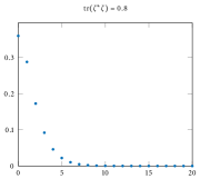
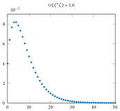
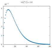
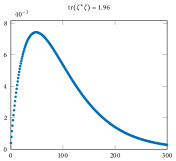
Figure 1: Distribution of total area for different values of $\operatorname{tr}(\zeta{{}^{*}}\zeta)$ when $\mathrm{rank}(\zeta)=2$.

Proposition 4 (Probability distribution of total area).

When $\zeta$ is of rank $2$ the probability distribution for the total area in the state $|\zeta\rangle$ is

$$P_{\zeta}(J)=\det({\bf 1}-\zeta{{}^{*}}\zeta)\left({\frac{1}{2}}\operatorname{tr}(\zeta{{}^{*}}\zeta)\right)^{J}(J+1),\quad J\in\mathbb{N}_{0}.$$

Proof of this proposition can be found in Appendix C.3. Plots for the probability distribution can be found in Fig. 1. Note how, as the non-zero eigenvalue of $\zeta{{}^{*}}\zeta$ approaches $1$ (or equivalently $\operatorname{tr}(\zeta{{}^{*}}\zeta)\rightarrow 2$), the relative shape of the distribution remains the same, which is a consequence of Proposition 3.

III.2.3 Relating $\operatorname{SO}^{*}(2N)$ and some Bogoliubov transformations

Some recent works by Bianchi and collaborators have emphasized the use of the symplectic group $\mathrm{Sp}(4N,\mathbb{R})$ to recover some interesting features for loop quantum gravity, such as anew parametrization of the loop variables Bianchi et al. (2016b, a). We would like now to coherent relate our states to this approach.

In fact, these states can be reinterpreted in terms of Bogoliubov transformations by making use of the connection between $\operatorname{SO}^{*}(2N)$ and the symplectic group $\mathrm{Sp}(4N,\mathbb{R})$. Recall that, if we have a set of $n$ decoupled harmonic oscillators

$$[C_{a},C^{\dagger}_{b}]=\delta_{ab},\quad[C_{a},C_{b}]=[C^{\dagger}_{a},C^{\dagger}_{b}]=0,$$ (101)

a Bogoliubov transformation is a a canonical transformation which maps them to a new set of harmonic oscillators,

$$\begin{pmatrix}\widetilde{C}\\ \widetilde{C}^{\dagger}\end{pmatrix}=\begin{pmatrix}U&V\\ \overline{V}&\overline{U}\end{pmatrix}\begin{pmatrix}C\\ C^{\dagger}\end{pmatrix}$$ (102)

The conditions on $U$ and $V$ such that

$$[\widetilde{C}_{a},\widetilde{C}^{\dagger}_{b}]=\delta_{ab},\quad[\widetilde{C}_{a},\widetilde{C}_{b}]=[\widetilde{C}^{\dagger}_{a},\widetilde{C}^{\dagger}_{b}]=0$$ (103)

are

$$UU^{\dagger}-VV^{\dagger}={\bf 1},\quad UV^{\textrm{t}}=VU^{\textrm{t}},$$ (104)

which automatically ensure that $U$ is invertible and that

$$\begin{pmatrix}U&V\\ \overline{V}&\overline{U}\end{pmatrix}\in\mathrm{Sp}(2n,\mathbb{R});$$ (105)

as such, we can interpret $\mathrm{Sp}(2n,\mathbb{R})$ as the group of Bogoliubov transformations of $n$ harmonic oscillators. The vacuum for the set of new harmonic oscillators is given by

$$|\widetilde{0}\rangle:=\mathcal{N}\exp\left({\frac{1}{2}}S^{ab}C^{\dagger}_{a}C^{\dagger}_{b}\right)|0\rangle,$$ (106)

also known as the squeezed vacuum, where $S$ is the symmetric matrix

$$S=-U^{-1}V.$$ (107)

In fact, it is easy to see that

$$\begin{split}C_{d}|\widetilde{0}\rangle&=\mathcal{N}\sum_{k=0}^{\infty}\frac{1}{k!}\left[C_{d},\left({\frac{1}{2}}S^{ab}C^{\dagger}_{a}C^{\dagger}_{b}\right)^{k}\right]|0\rangle=\mathcal{N}\sum_{k=0}^{\infty}\frac{1}{k!}k\left({\frac{1}{2}}S^{ab}C^{\dagger}_{a}C^{\dagger}_{b}\right)^{k-1}\left({\frac{1}{2}}S^{cd}C^{\dagger}_{c}+{\frac{1}{2}}S^{dc}C^{\dagger}_{c}\right)|0\rangle\\ &=\mathcal{N}\sum_{k=0}^{\infty}\frac{1}{k!}\left({\frac{1}{2}}S^{ab}C^{\dagger}_{a}C^{\dagger}_{b}\right)^{k}S^{dc}C^{\dagger}_{c}|0\rangle=S^{dc}C^{\dagger}_{c}|\widetilde{0}\rangle,\end{split}$$ (108)

from which it follows that

$$\widetilde{C}_{a}|\widetilde{0}\rangle=0.$$ (109)

The fact that $|\widetilde{0}\rangle$ has finite norm can be proven by evaluating $\langle\widetilde{0}|\widetilde{0}\rangle$ as a Gaussian integral, making use of the resolution of the identity in terms of the coherent states for the harmonic oscillators $C_{a}$.

In our framework, we use $n=2N$ harmonic oscillators, so we expect to deal with $\mathrm{Sp}(4N,\mathbb{R})$. To connect $\operatorname{SO}^{*}(2N)$ to the Bogoliubov transformations, note that $\operatorname{SO}^{*}(2N)$ can be embedded into $\mathrm{Sp}(4N,\mathbb{R})$ as

$$\varphi:\begin{pmatrix}X&Y\\ -\overline{Y}&\overline{X}\end{pmatrix}\in\operatorname{SO}{{}^{*}}(2N)\mapsto\begin{pmatrix}X&0&0&-Y\\ 0&X&Y&0\\ 0&-\overline{Y}&\overline{X}&0\\ \overline{Y}&0&0&\overline{X}\end{pmatrix}\in\mathrm{Sp}(4N,\mathbb{R}).$$ (110)

Indeed it is a simple exercise to show that the conditions (69) ensure that (104) hold. Hence we can interpret $\operatorname{SO}^{*}(2N)$ as a subgroup of Bogoliubov transformations of the $2N$ harmonic oscillators $A_{a}$, $B_{b}$ that we use to construct the Jordan-Schwinger representation. In particular, for the Bogoliubov transformation $\varphi(g_{\zeta}^{-1})$, with $\zeta\in\Omega_{N}$ we get

$$S=\begin{pmatrix}0&-\zeta\\ \zeta&0\end{pmatrix},$$ (111)

so that the associated squeezed vacuum (106) is

$$\mathcal{N}\exp\left({\frac{1}{2}}S^{ab}B^{\dagger}_{a}A^{\dagger}_{b}\right)|0\rangle=\mathcal{N}\exp\left({\frac{1}{2}}\zeta^{ab}\widetilde{F}_{ab}\right)|0\rangle,$$ (112)

which is exactly the coherent state $|\zeta\rangle$. To summarise, we can regard the new coherent intertwiners we defined as the squeezed vacua associated to a subgroup of Bogoliubov transformations, isomorphic to $\operatorname{SO}^{*}(2N)$. The particular Bogoliubov transformations are exactly those for which the squeezed vacuum is still $\mathrm{SU}(2)$ invariant (i.e, an intertwiner), so that we can essentially regard $\operatorname{SO}^{*}(2N)$ as the group of canonical transformations of $2N$ harmonic oscillators preserving $\mathrm{SU}(2)$ invariance, where the $\mathrm{SU}(2)$ action is implemented through the Jordan-Schwinger representation.

III.3 Semi-classical limit

Let us now consider the semi-classical limit of our coherent intertwiners. Our goal is to obtain out of the expectation values of the algebra generators a set of variables that, endowed with the appropriate Poisson structure, we can interpret as a classical geometry (similarly to what we discussed in Section I). In particular, we want to be able to construct a set of vectors that sum to zero, and as such can be regarded as the normals to a convex polyhedron Borja et al. (2011).

III.3.1 Recovering the spinor variables

In order to investigate the semi-classical limit, it will prove useful to rewrite the expected values of the ${\mathfrak{so}}^{*}(2N)$ generators (99) in a different way. Note the similarity with the bra-ket notation we introduced in section I when working with classical spinors.

Proposition 5.

The expectation values of the ${\mathfrak{so}}^{*}(2N)$ generators can be written in the form

$$\langle\zeta|F_{ab}|\zeta\rangle=\sum_{\alpha=1}^{k}\frac{1}{\lambda_{\alpha}}[z^{\alpha}_{a}|z^{\alpha}_{b}\rangle,\quad\langle\zeta|\widetilde{F}_{ab}|\zeta\rangle=\sum_{\alpha=1}^{k}\frac{1}{\lambda_{\alpha}}\langle z^{\alpha}_{a}|z^{\alpha}_{b}],\quad\langle\zeta|E_{ab}|\zeta\rangle=\delta_{ab}+\sum_{\alpha=1}^{k}\langle z^{\alpha}_{a}|z^{\alpha}_{b}\rangle,$$

where $k={\frac{1}{2}}\mathrm{rank}(\zeta)$, $\lambda_{\alpha}^{2}$ is a non-zero eigenvalue of $\zeta{{}^{*}}\zeta$ and the spinors are specified in terms of a unitary matrix $U$,

$$|z^{\alpha}_{a}\rangle=\left(\frac{2\lambda^{2}_{\alpha}}{1-\lambda_{\alpha}^{2}}\right)^{{\frac{1}{2}}}\begin{pmatrix}U_{a,2\alpha-1}\\ U_{a,2\alpha}\end{pmatrix}\textrm{ with }\zeta=UMU^{\textrm{t}}\textrm{ and }M=\bigoplus_{\alpha=1}^{k}\lambda_{\alpha}\begin{pmatrix}0&-1\\ 1&0\end{pmatrix}\oplus{\bf 0}_{N-2k},\quad\lambda_{\alpha}>0.$$ (113)

As such the spinors satisfy automatically some closure constraint

$$\sum_{a=1}^{n}|z^{\alpha}_{a}\rangle\langle z^{\beta}_{a}|=\delta_{\alpha\beta}\sum_{a=1}^{n}{\frac{1}{2}}\langle z^{\alpha}_{a}|z^{\alpha}_{a}\rangle{\bf 1}_{2}.$$

Proof.

Since $\zeta$ is an antisymmetric matrix, we know that $\zeta=UMU^{\textrm{t}}$, where $U$ is unitary and

$$M=\bigoplus_{\alpha=1}^{k}\lambda_{\alpha}\begin{pmatrix}0&-1\\ 1&0\end{pmatrix}\oplus{\bf 0}_{N-2k},\quad\lambda_{\alpha}>0.$$ (114)

As a consequence,

$$M{{}^{*}}M=\bigoplus_{\alpha=1}^{k}\lambda_{\alpha}^{2}{\bf 1}_{2}\oplus{\bf 0}_{N-2k}\textrm{ and }({\bf 1}-M{{}^{*}}M)^{-1}=\bigoplus_{\alpha=1}^{k}(1-\lambda_{\alpha}^{2})^{-1}\,{\bf 1}_{2}\oplus{\bf 1}_{N-2k}.$$ (115)

It follows that

$$\langle\zeta|F_{ab}|\zeta\rangle = \left[2\zeta({\bf 1}-\zeta{{}^{*}}\zeta)^{-1}\right]_{ab}=\left[2UM({\bf 1}-M{{}^{*}}M)^{-1}U^{\textrm{t}}\right]_{ab}=\sum_{\alpha=1}^{k}\sum_{c,d=1}^{N}\frac{2\lambda_{\alpha}}{1-\lambda_{\alpha}^{2}}U_{ac}\left(\delta_{c,2\alpha}\delta_{d,2\alpha-1}-\delta_{c,2\alpha-1}\delta_{d,2\alpha}\right)U_{bd}$$ (116)

$$= \sum_{\alpha=1}^{k}\frac{2\lambda_{\alpha}}{1-\lambda_{\alpha}^{2}}\left(U_{a,2\alpha}U_{b,2\alpha-1}-U_{a,2\alpha-1}U_{b,2\alpha}\right)$$

and

$$\langle\zeta|E_{ab}|\zeta\rangle-\delta_{ab} = \left[2\zeta{{}^{*}}\zeta({\bf 1}-\zeta{{}^{*}}\zeta)^{-1}\right]_{ab}=\left[2\overline{U}M{{}^{*}}M({\bf 1}-M{{}^{*}}M)^{-1}U^{\textrm{t}}\right]_{ab}$$ (117)

$$= \sum_{\alpha=1}^{k}\sum_{c,d=1}^{N}\frac{2\lambda_{\alpha}^{2}}{1-\lambda_{\alpha}^{2}}\overline{U}_{ac}\left(\delta_{c,2\alpha-1}\delta_{d,2\alpha-1}+\delta_{c,2\alpha}\delta_{d,2\alpha}\right)U_{bd}$$ (118)

$$= \sum_{\alpha=1}^{k}\frac{2\lambda_{\alpha}^{2}}{1-\lambda_{\alpha}^{2}}\left(\overline{U}_{a,2\alpha-1}U_{b,2\alpha-1}+\overline{U}_{a,2\alpha}U_{b,2\alpha}\right).$$ (119)

Choosing

$$|z^{\alpha}_{a}\rangle=\left(\frac{2\lambda^{2}_{\alpha}}{1-\lambda_{\alpha}^{2}}\right)^{{\frac{1}{2}}}\begin{pmatrix}U_{a,2\alpha-1}\\ U_{a,2\alpha}\end{pmatrix}\quad\Rightarrow\quad|z^{\alpha}_{a}]=\left(\frac{2\lambda^{2}_{\alpha}}{1-\lambda_{\alpha}^{2}}\right)^{{\frac{1}{2}}}\begin{pmatrix}\overline{U}_{a,2\alpha}\\ -\overline{U}_{a,2\alpha-1}\end{pmatrix}$$ (120)

we find

$$\langle\zeta|F_{ab}|\zeta\rangle=\sum_{\alpha=1}^{k}\frac{1}{\lambda_{\alpha}}[z^{\alpha}_{a}|z^{\beta}_{b}\rangle,\quad\langle\zeta|E_{ab}|\zeta\rangle=\delta_{ab}+\sum_{\alpha=1}^{n}\langle z^{\alpha}_{a}|z^{\alpha}_{b}\rangle.$$ (121)

Moreover, we have the closure constraints

$$\sum_{a=1}^{N}|z^{\alpha}_{a}\rangle\langle z^{\beta}_{a}| = \left(\frac{2\lambda^{2}_{\alpha}}{1-\lambda_{\alpha}^{2}}\right)^{{\frac{1}{2}}}\left(\frac{2\lambda^{2}_{\beta}}{1-\lambda_{\beta}^{2}}\right)^{{\frac{1}{2}}}\sum_{a=1}^{N}\begin{pmatrix}U_{a,2\alpha-1}\overline{U}_{a,2\beta-1}&U_{a,2\alpha}\overline{U}_{a,2\beta-1}\\ U_{a,2\alpha-1}\overline{U}_{a,2\beta}&U_{a,2\alpha}\overline{U}_{a,2\beta}\end{pmatrix}$$ (122)

$$= \delta_{\alpha\beta}\frac{2\lambda^{2}_{\alpha}}{1-\lambda_{\alpha}^{2}}{\bf 1}_{2}=\delta_{\alpha\beta}\sum_{a=1}^{N}{\frac{1}{2}}\langle z^{\alpha}_{a}|z^{\alpha}_{a}\rangle{\bf 1}_{2}$$

as expected. ∎

As consequence of this fact, in the limit $\lambda_{\alpha}\rightarrow 1,\quad\alpha=1,\dotsc,k$ where the expected value of the total area

$$\langle\mathcal{A}\rangle=\sum_{\alpha=1}^{k}\frac{\lambda_{\alpha}^{2}}{1-\lambda_{\alpha}^{2}}\rightarrow\infty,$$ (123)

we have

$$\langle\zeta|F_{ab}|\zeta\rangle\sim\sum_{\alpha=1}^{k}[z^{\alpha}_{a}|z^{\alpha}_{b}\rangle=\sum_{\alpha=1}^{k}f_{ab}^{\alpha},\quad\langle\zeta|E_{ab}|\zeta\rangle=\delta_{ab}+\sum_{\alpha=1}^{k}\langle z^{\alpha}_{a}|z^{\alpha}_{b}\rangle=\delta_{ab}+\sum_{\alpha=1}^{k}e_{ab}^{\alpha}.$$ (124)

We can interpret the semi-classical limit as a classical geometry by introducing the canonical Poisson structure on $\mathbb{C}^{2kN}$ which is, using the coordinates $|z^{\alpha}_{a}\rangle=\left(\begin{array}[]{c}x^{\alpha}_{a}\\ y^{\alpha}_{a}\end{array}\right)$,

$$\{x^{\alpha}_{a},\overline{x}^{\beta}_{b}\}=\{y^{\alpha}_{a},\overline{y}^{\beta}_{b}\}=-i\delta^{\alpha\beta}\delta_{ab}$$ (125)

with all other brackets vanishing. With this Poisson structure, the functions

$$e_{ab}:=\sum_{\alpha=1}^{k}\langle z^{\alpha}_{a}|z^{\alpha}_{b}\rangle=\sum_{\alpha=1}^{k}e_{ab}^{\alpha},\quad f_{ab}:=\sum_{\alpha=1}^{k}[z^{\alpha}_{a}|z^{\alpha}_{b}\rangle=\sum_{\alpha=1}^{k}f_{ab}^{\alpha}$$ (126)

satisfy

$$\{e_{ab},e_{cd}\} =-i\left(\delta_{cb}e_{ad}-\delta_{ad}e_{cb}\right),\quad\{e_{ab},f_{cd}\}=-i\left(\delta_{ad}f_{bc}-\delta_{ac}f_{bd}\right),\quad\{f_{ab},f_{cd}\}=\{\overline{f}_{\!ab},\overline{f}_{\!cd}\}=0,$$ (127a)

$$\{e_{ab},\overline{f}_{\!cd}\} =-i\left(\delta_{bc}\overline{f}_{\!ad}-\delta_{bd}\overline{f}_{\!ac}\right),\quad\{f_{ab},\overline{f}_{\!cd}\}=-i\left(\delta_{db}e_{ca}+\delta_{ca}e_{db}-\delta_{cb}e_{da}-\delta_{da}e_{cb}\right),$$ (127b)

which are the classical analogue of the ${\mathfrak{so}}^{*}(2N)$ commutation relations (76).

III.3.2 Geometric interpretation of the semi-classical states

We would like now to determine whether the spinorial formalism we have recovered actually allows the reconstruction of a polyhedron or of anything else.

The rank of the matrix parametrizing the coherent state actually determines the number of spinors we recover. As we already recalled, the rank of $\zeta$ is at most $N$, and since $\zeta$ is an antisymmetric matrix its rank has to be even. We noted it $2k$. In the semi-classical limit we have recovered $2kN$ spinors.

Let us consider the case $k=1$, that is $\mathrm{rank}(\zeta)=2$ to start. In fact it is this case that was always considered until now in the literature Bonzom and Livine (2013); Freidel and Hnybida (2013, 2014); Bonzom et al. (2016). In this case, we recover exactly the standard spinorial parametrization of the convex polyhedron since we recover $2N$ spinors. Indeed there is no sum to consider in (126) and (122) states that the closure constraint is satisfied. Hence we recover in this case, a convex polyhedron in the semi-classical limit.

The cases $k>1$ are more subtle. Indeed, we recover more spinors than we started with. We can expect different interpretations of the resulting construction, bearing in mind that we have $k$ closure constraints in (122).

• We recover a polyhedron with $kN$ faces, such that the normal of the faces cancel by bundle of $N$ (think of the cube, where the six normals cancel by bundle of two). Since we can define some total observables as in (126), this $kN$ faces polyhedron could be coarse-grained as a polyhedron with $N$ faces.

• We recover a set of k polyhedra with $N$ faces, which could be coarse-grained as a polyhedron with $N$ faces thanks to (126), or not.

• We do not really recover anything close to a finite set of polyhedra.

To assess what we really obtained, we need to check what are the symmetry transformations of the set of spinors we have reconstructed.

Proposition 6.

The unitary matrix $U$ in the decomposition

$$\zeta=UMU^{\textrm{t}}$$

is defined up to a unitary transformation $W$

$$U\rightarrow UW,\quad W\in\bigtimes_{i=1}^{\ell}\mathrm{Sp}(2\mu_{i})\times\mathrm{U}(N-2k),$$

where $\ell$ is the number of distinct $\lambda_{\alpha}$ in the decomposition of $\zeta$ and the $\mu_{i}$ are the multiplicities of each distinct $\lambda_{\alpha}$. $\mathrm{Sp}(2\mu_{i})$ is the compact symplectic group. When all the $\lambda_{\alpha}$ are distinct this reduces to

$$V\in\mathrm{SU}(2)^{\times k}\times\mathrm{U}(N-2k).$$

Since the proof is a bit lengthy, we postpone it to Appendix D. From the definition of the spinors, the relevant symmetries we need to consider are given by $\mathrm{Sp}(2\mu_{i})$. The left-over, given by $\operatorname{U}(N-2k)$, does not affect the definition of the spinors. The symmetries we have identified, together with the closure constraints (122), allow us to interpret the nature of the geometric structures we recover in the semi-classical limit.

First note that when there is only one $\lambda$, that is $\mathrm{rank}(\zeta)=2$, we trivially recover only one copy of $\mathrm{SU}(2)$ which is the global symmetry of the polyhedron. Indeed, it is defined only up to a global rotation. Furthermore the observables $e_{ab},f_{ab},\tilde{f}_{ab}$ are invariant under such transformations. This is consistent with the fact that we recovered a single polyhedron.

Second, when all the $\lambda_{\alpha}$’s are distinct, we have $k$ global $\mathrm{SU}(2)$ symmetries, together with $k$ closure constraints. This indicates that we have in general not one polyhedron but a set of $k$ polyhedra with $N$ faces. The observables $e_{ab}^{\alpha},f_{ab}^{\alpha},\tilde{f}_{ab}^{\alpha}$ are invariant under each of these global $\mathrm{SU}(2)$ transformations. For a given $\alpha$, these observables correspond to the observables for a given polyhedron $\alpha$. The new set of observables is hence generated by $k$ copies of ${\mathfrak{so}}^{*}(2N)$. The geometry of each of these polyhedra can be reconstructed from the knowledge of the observables as usual.

One might then wonder whether the definition of the diagonal ${\mathfrak{so}}^{*}(2N)$ from (126) allows to coarse-grain the set of $k$ polyhedra with $N$ faces to a single new $N$ faces polyhedron. As the following proposition shows, the answer is negative: the diagonal ${\mathfrak{so}}^{*}(2N)$ observables do not allow to reconstruct a polyhedron that is closed.

Proposition 7.

Consider $k$ convex $N$ faces polyhedra indexed by $\alpha$ and their associated algebra ${\mathfrak{so}}^{*}(2N)$ of observables spanned by $e_{ab}^{\alpha},f_{ab}^{\alpha},\tilde{f}_{ab}^{\alpha}$. The diagonal subalgebra ${\mathfrak{so}}^{*}(2N)$ spanned by $e_{ab}=\sum_{\alpha=1}^{k}e_{ab}^{\alpha},f_{ab}=\sum_{\alpha=1}^{k}f_{ab}^{\alpha},\tilde{f}_{ab}=\sum_{\alpha=1}^{k}\tilde{f}_{ab}^{\alpha}$ is not the algebra of observables of a single closed polyhedron.

Proof.

Since we deal with polyhedra, we have the closure constraints

$$\sum_{a=1}^{N}|z^{\alpha}_{a}\rangle\langle z^{\beta}_{a}| = \delta_{\alpha\beta}\sum_{a=1}^{N}{\frac{1}{2}}\langle z^{\alpha}_{a}|z^{\alpha}_{a}\rangle{\bf 1}_{2}=\Lambda_{\alpha}{\bf 1}_{2}.$$ (128)

where $\Lambda_{\alpha}$ is half of the total area of the polyhedron $\alpha$,

$$\sum_{a=1}^{N}\langle z^{\alpha}_{a}|z^{\alpha}_{a}\rangle=\sum_{a=1}^{N}e_{aa}^{\alpha}=2\Lambda_{\alpha}.$$ (129)

Let us now consider the normals $\vec{V}_{a}$ of the coarse-grained polyhedron. By construction, the relative angles between the normals are given by

$$\vec{V}_{a}\cdot\vec{V}_{b}={\frac{1}{2}}e_{ab}e_{ba}-\frac{1}{4}e_{aa}e_{bb}.$$ (130)

If the closure constraint $\sum_{a}\vec{V}_{a}=0$ is satisfied then we also have that $\sum_{ab}\vec{V}_{a}\cdot\vec{V}_{b}=0$. Hence we are supposed to show that

$$\sum_{ab}\left({\frac{1}{2}}e_{ab}e_{ba}-\frac{1}{4}e_{aa}e_{bb}\right)=0.$$ (131)

Using the definition of the coarse-grained $e_{ab}$ in terms of the $e_{ab}^{\alpha}$ we have

$$\sum_{ab}e_{ab}e_{ba} = \sum_{ab\alpha\beta}\langle z^{\alpha}_{a}|z^{\alpha}_{b}\rangle\langle z^{\beta}_{b}|z^{\beta}_{a}\rangle=\sum_{a\alpha\beta}\delta_{\alpha\beta}\Lambda_{\alpha}\langle z^{\alpha}_{a}|z^{\beta}_{a}\rangle=2\sum_{\alpha}\Lambda_{\alpha}^{2},$$ (132)

$$\sum_{ab}e_{aa}e_{bb} = \left(\sum_{a}e_{aa}\right)^{2}=\left(\sum_{a\alpha}e^{\alpha}_{aa}\right)^{2}=\left(2\sum_{\alpha}\Lambda_{\alpha}\right)^{2}=4\sum_{\alpha\beta}\Lambda_{\alpha}\Lambda_{\beta}.$$ (133)

We deduce then that

$$\sum_{ab}\left({\frac{1}{2}}e_{ab}e_{ba}-\frac{1}{4}e_{aa}e_{bb}\right)=\sum_{\alpha}\Lambda_{\alpha}^{2}-\sum_{\alpha\beta}\Lambda_{\alpha}\Lambda_{\beta}=-\sum_{\alpha\neq\beta}\Lambda_{\alpha}\Lambda_{\beta}<0,$$ (134)

since $\Lambda_{\alpha}>0$. Hence the closure constraint is not satisfied and we do not have a coarse-grained polyhedron. ∎

Hence when all the $\lambda_{\alpha}$’s are distinct, we have a collection of $k$ polyhedra with $N$ faces, which cannot be seen as a unique polyhedron. One could try use a boost to make the spinors close as explained extensively in Livine (2013). This however would not close the polyhedron: an overall $X\in\operatorname{SL}(2,\mathbb{C})$ transformation of the spinors would preserve the matrix $\zeta$, but it would only have the effect of transforming the areas as

$$\Lambda_{\alpha}\rightarrow\Lambda^{\prime}_{\alpha}=\sum_{a=1}^{n}\langle z^{\alpha}_{a}|\overline{X}X^{\textrm{t}}|z^{\alpha}_{a}\rangle>0.$$ (135)

Repeating the steps from the proof of Proposition 7, in particular (134), shows that the transformed polyhedron does not close as well.

Finally, when the $\lambda_{\alpha}$ appear with multiplicities, we do not have a discrete family of polyhedra. The compact symplectic group symmetries do not leave invariant the observables $e_{ab}^{\alpha},f_{ab}^{\alpha},\tilde{f}_{ab}^{\alpha}$, though the total observables $e_{ab},f_{ab},\tilde{f}_{ab}$ are invariant by construction. Given a fixed value of the $|z^{\alpha}_{a}\rangle$, we can reconstruct a polyhedron $\alpha$ with $N$ faces, which will have a global symmetry given by $\mathrm{SU}(2)$. Hence we can get in this way $k$ polyhedra with $N$ faces. However performing a transformation in $\bigtimes_{i=1}^{\ell}\mathrm{Sp}(2\mu_{i})/\mathrm{SU}(2)^{\times k}$ will give different values for the $|z^{\alpha}_{a}\rangle$ (essentially mixing spinors associated to different polyhedra) and the new polyhedra will be totally different than the previous ones when the multiplicity $\mu_{i}$ is higher than 1. Hence the semi-classical limit in this case can be seen as a set of families of polyhedra given by the coset

$$\bigtimes_{i=1}^{\ell}\mathrm{Sp}(2\mu_{i})/\mathrm{SU}(2)^{\times k}.$$ (136)

Note that some families can be only with a unique element, whereas some others can have a continuum of polyhedra. For example, let us consider an intertwiner with $N$ legs, such that $N>7$, with $\zeta$ of rank 8 (hence $k=4$) and $\lambda_{1}=\lambda_{2}$, so $\mu=2$ we have (recalling that $\mathrm{Sp}(2)=\mathrm{SU}(2)$)

$$\left(\mathrm{Sp}(2\mu)\times\mathrm{Sp}(2)\times\mathrm{Sp}(2)\right)/\mathrm{SU}(2)^{\times 4}=\left(\mathrm{Sp}(4)\times\mathrm{Sp}(2)\times\mathrm{Sp}(2)\right)/\mathrm{SU}(2)^{\times 4}=\mathrm{Sp}(4)/\mathrm{SU}(2)^{\times 2}.$$

Hence we have two $N$ faces polyhedra, with total area specified by $\lambda_{3}$ and $\lambda_{4}$, and a continuous family of 2 polyhedra, with $N$ faces, with each polyhedron a total area specified by $\lambda_{1}$.

As a more explicit example let us consider now a 4 legs intertwiner, with $\zeta$ of rank 4 (hence $k=2$) and $\lambda_{1}=\lambda_{2}=\sqrt{\frac{1}{2}}$. We take explicitly for $\zeta$

$$\zeta={\frac{1}{2}}U\begin{pmatrix}\sigma&0\\ 0&\sigma\end{pmatrix}U^{\textrm{t}}\textrm{ with }U={\frac{1}{2}}\left(\begin{array}[]{cccc}1&1&\sqrt{{\frac{1}{2}}}(-1-i)&\sqrt{{\frac{1}{2}}}(-1+i)\\ 1&-1&\sqrt{{\frac{1}{2}}}(1-i)&\sqrt{{\frac{1}{2}}}(1+i)\\ i&1&0&\sqrt{2}\\ -i&1&\sqrt{2}&0\end{array}\right)$$ (137)

From the unitary $U$, we can identify the spinors

$$|z_{1}^{1}\rangle=\left(\begin{array}[]{c}{\frac{1}{2}}\\ {\frac{1}{2}}\end{array}\right),\,|z_{2}^{1}\rangle=\left(\begin{array}[]{c}{\frac{1}{2}}\\ -{\frac{1}{2}}\end{array}\right),\,|z_{3}^{1}\rangle=\left(\begin{array}[]{c}\frac{i}{2}\\ \frac{i}{2}\end{array}\right),\,|z_{4}^{1}\rangle=\left(\begin{array}[]{c}-\frac{i}{2}\\ \frac{i}{2}\end{array}\right),$$ (146)

$$|z_{1}^{2}\rangle=\frac{\sqrt{2}}{4}\left(\begin{array}[]{c}-1-i\\ -1+i\end{array}\right),\,|z_{2}^{2}\rangle=\frac{\sqrt{2}}{4}\left(\begin{array}[]{c}1-i\\ 1+i\end{array}\right),\,|z_{3}^{2}\rangle=\left(\begin{array}[]{c}0\\ \sqrt{{\frac{1}{2}}}\end{array}\right),\,|z_{4}^{2}\rangle=\left(\begin{array}[]{c}0\\ \sqrt{\frac{1}{2}}\end{array}\right),$$ (155)

which in turn generate the normals that tell us about the two polyhedra geometries.

$$\vec{V}^{1}_{1}=\left(\begin{array}[]{c}\frac{1}{4}\\ 0\\ 0\end{array}\right),\,\vec{V}^{1}_{2}=\left(\begin{array}[]{c}-\frac{1}{4}\\ 0\\ 0\end{array}\right),\,\vec{V}^{1}_{3}=\left(\begin{array}[]{c}0\\ -\frac{1}{4}\\ 0\end{array}\right),\,\vec{V}^{1}_{4}=\left(\begin{array}[]{c}0\\ \frac{1}{4}\\ 0\end{array}\right),$$ (168)

$$\vec{V}^{2}_{1}=\left(\begin{array}[]{c}0\\ -\frac{1}{4}\\ 0\end{array}\right),\,\vec{V}^{2}_{2}=\left(\begin{array}[]{c}0\\ \frac{1}{4}\\ 0\end{array}\right),\,\vec{V}^{2}_{3}=\left(\begin{array}[]{c}0\\ 0\\ -\frac{1}{4}\end{array}\right),\,\vec{V}^{2}_{4}=\left(\begin{array}[]{c}0\\ 0\\ -\frac{1}{4}\end{array}\right),$$ (181)

We note that the the two tetrahedra are actually both degenerated. Let us now perform a unitary transformation given by $U{\rightarrow}UW$, with $W\in\mathrm{Sp}(4)$, which leaves $M$ invariant as it is easy to check.

$$W=\sqrt{\frac{1}{2}}\left(\begin{array}[]{cc}{\bf 1}_{2}&{\bf 1}_{2}\\ {\bf 1}_{2}&-{\bf 1}_{2}\end{array}\right),\quad{\rightarrow}\quad|\tilde{z}^{\pm}_{a}\rangle=\sqrt{\frac{1}{2}}\left(|z^{1}_{a}\rangle\pm|z^{2}_{a}\rangle\right)$$ (182)

Skipping the explicit expression of the spinors, we get the normals given by

$$\vec{V}_{1}^{\pm}=\frac{1}{8}\left(\begin{array}[]{c}1\mp\sqrt{2}\\ -1\pm\sqrt{2}\\ 0\end{array}\right),\,\vec{V}_{2}^{\pm}=\frac{1}{8}\left(\begin{array}[]{c}-1\\ 1\\ \pm\sqrt{2}\end{array}\right),\,\vec{V}^{\pm}_{3}=\frac{1}{8}\left(\begin{array}[]{c}0\\ -1\mp\sqrt{2}\\ -1\mp\sqrt{2}\end{array}\right),\,\vec{V}^{\pm}_{4}=\frac{1}{8}\left(\begin{array}[]{c}\pm\sqrt{2}\\ 1\\ 1\end{array}\right).$$ (195)

We note now that the two polyhedra, indexed by $\pm$ are non-degenerated. The area of the faces changed, as one can easily check by evaluating the norm of the normals, but not their respective total area.

So to summarize, when the $\lambda_{\alpha}$ have some multiplicity, we cannot associate a discrete set of polyhedra to a single coherent state, instead we have to consider a continuum of polyhedra. In a sense the standard picture of the semi-classical limit breaks down.

It is quite interesting that the degenerate structure appears as soon as the semi-classical polyhedra have the same total area specified by the $\lambda_{\alpha}$. The fact that they might look very different, with individual faces of different values for the area does not affect the degeneracy.

Discussion

We have identified the algebra of observables for a $\mathrm{SU}(2)$ intertwiner to be ${\mathfrak{so}}^{*}(2N)$ and constructed the associated coherent states. We studied the semi-classical limit of these coherent states which happened to be more subtle than the previously constructed coherent states of a $\mathrm{SU}(2)$ intertwiner Livine and Tambornino (2012). According to the nature of the matrix parametrizing the coherent state, the semi-classical limit can give rise to families of convex polyhedra with $N$ faces that can be discrete (ie with a single polyhedron) or continuous (ie with an infinite number of polyhedra). The nature of the family, being discrete of continuous is characterized by the value of the total area of the polyhedron. If at least two polyhedra have the same total area, we will get a continuum of polyhedra with the same total area.

The $\operatorname{SO}^{*}(2N)$ states we have introduced have already been discovered in the literature Bonzom and Livine (2013); Freidel and Hnybida (2013, 2014); Bonzom et al. (2016); Bianchi et al. (2016b), motivated by different reasons. However these states were always defined in terms of a matrix of rank 2, which is in the semi-classical limit the best scenario, since we only get one polyhedron in this case. It would be interesting to see how the results of Bonzom and Livine (2013); Freidel and Hnybida (2013, 2014); Bonzom et al. (2016); Bianchi et al. (2016b) are affected when dealing with a more general coherent state.

There are some obvious generalizations to consider.

First, the algebra of observables has been deformed to the quantum group case, to deal with ${\mathcal{U}}_{q}(\mathfrak{su}(2))$ intertwiners Dupuis and Girelli (2014). Hence the deformed algebra ${\mathcal{U}}_{q}({\mathfrak{so}}^{*}(2N))$ has been identified (not the co-algebra sector though). It would be interesting to see how the coherent states are generalized in this case. When $q$ is real, since the representation theory of ${\mathcal{U}}_{q}(\mathfrak{su}(2))$ is very similar in a sense to the one of ${\mathcal{U}}(\mathfrak{su}(2))$, we might not expect some great differences, either to define the coherent states or in term of the semi-classical limit. The case $q$ root of unity might be more interesting since the representation theory then changes drastically. This could affect somehow the semi-classical limit. This is to be explored.

Another interesting generalization would be the Lorentzian case. The spinorial formalism has been generalized to deal with $\mathrm{SU}(1,1)$ intertwiners Sellaroli (2015); Girelli and Sellaroli (2015). This formalism is more subtle than the Euclidian case, since when dealing with continuous representations, the ”observables” acting on an intetwiner defined in terms of unitary irreps might not give an intertwiner defined in terms of unitary irreps. Nevertheless the algebra of observables can be defined. It would be interesting to see whether we can do some similar calculations as done here. We leave this for later investigations.

Appendix A Perelomov coherent states

Recall that generalised coherent states for a unitary irreducible module $V$ of a generic Lie Group $G$ are defined as

$$|g\rangle:=g|\psi_{0}\rangle,\quad g\in G,$$ (196)

where $|\psi_{0}\rangle\in V$ is a fixed state of norm $1$. Note that, at this stage, there is no guarantee that two coherent states labelled by different group elements indeed describe physically different states (i.e., they are not the same vector up to a phase). In fact, let $H\subseteq G$ be the maximal subgroup that leaves $|\psi_{0}\rangle$ invariant up to a phase, that is

$$h|\psi_{0}\rangle=e^{i\theta(h)}|\psi_{0}\rangle,\quad\forall h\in H,$$ (197)

which will be called the isotropy subgroup for $|\psi_{0}\rangle$: it is obvious that if $g_{2}\in g_{1}H$ then

$$|g_{2}\rangle=e^{i\theta}|g_{1}\rangle,$$ (198)

i.e., the two states are equivalent. The inequivalent coherent states are labelled by elements of the left coset space

$$G/H:=\{gH{\,|\,}g\in G\},$$ (199)

and are given by

$$|x\rangle:=|g_{x}\rangle=g_{x}|\psi_{0}\rangle,\quad\forall x\in G/H,$$ (200)

where $g_{x}\in x$ is a representative of the equivalence class $x$.

Appendix B Proof of Proposition 1

First recall that the exponential map of $\operatorname{GL}(N,\mathbb{C})$ is surjective, so that any element of $\operatorname{GL}(N,\mathbb{C})$ can be written in the form $e^{E_{\alpha}}\equiv e^{\alpha}$, for some $\alpha\in M_{n}(\mathbb{C})$. Using the fact that

$$e^{-E_{\alpha}}|0\rangle=e^{-\operatorname{tr}(\alpha)}|0\rangle=\frac{1}{\det(e^{\alpha})}|0\rangle$$ (201)

and

$$\widetilde{F}_{12}\equiv{\frac{1}{2}}\widetilde{F}_{\xi_{0}},$$ (202)

we can write

$$e^{E_{\alpha}}|\psi_{J}\rangle=\frac{\det(e^{\alpha})}{\sqrt{J!(J+1)!}}e^{E_{\alpha}}({\frac{1}{2}}\widetilde{F}_{\xi_{0}})^{J}e^{-E_{\alpha}}|0\rangle\equiv\frac{\det(e^{\alpha})}{\sqrt{J!(J+1)!}}\big{(}{\frac{1}{2}}e^{E_{\alpha}}\widetilde{F}_{\xi_{0}}e^{-E_{\alpha}}\big{)}^{J}|0\rangle.$$ (203)

Using the well known formula

$$e^{A}Be^{-A}=B+[A,B]+\frac{1}{2!}[A,[A,B]]+\frac{1}{3!}[A,[A,[A,B]]]+\dotsb$$ (204)

and the commutation relation

$$[E_{\alpha},\widetilde{F}_{z}]=\widetilde{F}_{\alpha z+z\alpha^{\textrm{t}}}$$ (205)

we eventually find that

$$e^{E_{\alpha}}|\psi_{J}\rangle=\frac{\det(e^{\alpha})}{\sqrt{J!(J+1)!}}\left({\frac{1}{2}}\widetilde{F}_{e^{\alpha}\xi_{0}e^{\alpha^{\textrm{t}}}}\right)^{J}|0\rangle$$ (206)

as expected.

Appendix C Proof of the Propositions of Section III.2.2

The easiest way to compute the matrix elements of the ${\mathfrak{so}}{{}^{*}}(2N)$ generators $E_{ab}$, $F_{ab}$ and $\widetilde{F}_{ab}$ in the coherent state basis is to make use of the $2N$ harmonic oscillator operators $A_{a}$, $B_{a}$; in particular, we are going to project the states $|\zeta\rangle$ on the well-known harmonic oscillator coherent states. Recall that (Perelomov, 1986, chap. 3) coherent states for the representation of the Heisenberg group $\mathrm{H}_{2N}$ with generators satisfying

$$\left[A_{a},A^{\dagger}_{b}\right]=\left[B_{a},B^{\dagger}_{b}\right]=\delta_{ab}{\bf 1},$$ (207)

acting on the vector space spanned by the vectors

$$|\mu,\nu\rangle=\frac{\left(A^{\dagger}\right)^{\mu}}{\sqrt{\mu!}}\frac{\left(B^{\dagger}\right)^{\nu}}{\sqrt{\nu!}}|0\rangle,\quad\mu,\nu\in\mathbb{N}_{0},$$ (208)

where $|0\rangle\equiv|0,0\rangle$ is the harmonic oscillator vacuum

$$A_{a}|0\rangle=B_{a}|0\rangle=0,$$ (209)

are the vectors

$$|\alpha,\beta\rangle:=e^{-{\frac{1}{2}}\left(\alpha{{}^{*}}\alpha+\beta{{}^{*}}\beta\right)}\sum_{\mu,\nu\in\mathbb{N}_{0}^{N}}\frac{\alpha^{\mu}}{\sqrt{\mu!}}\frac{\beta^{\nu}}{\sqrt{\nu!}}|\mu,\nu\rangle,\quad\alpha,\beta\in\mathbb{C}^{N}$$ (210)

satisfying

$$A_{a}|\alpha,\beta\rangle=\alpha_{a}|\alpha,\beta\rangle,\quad B_{a}|\alpha,\beta\rangle=\beta_{a}|\alpha,\beta\rangle.$$ (211)

The resolution of the identity in terms of these coherent states is given by

$$\int_{\mathbb{C}^{2N}}{\textrm{d}}\mu(\alpha,\beta)|\alpha,\beta\rangle\langle\alpha,\beta|={\bf 1},$$ (212)

where the measure of integration is

$${\textrm{d}}\mu(\alpha,\beta)=\frac{1}{\pi^{2n}}{\textrm{d}}^{n}\Re(\alpha)\,{\textrm{d}}^{n}\,\Im(\alpha)\,{\textrm{d}}^{n}\Re(\beta)\,{\textrm{d}}^{n}\,\Im(\beta).$$ (213)

We can now use the fact that

$$\begin{split}\langle\alpha,\beta|\zeta\rangle&=\mathcal{N}(\zeta)\,\langle\alpha,\beta|\exp\left({\frac{1}{2}}\widetilde{F}_{\zeta}\right)|0\rangle=\mathcal{N}(\zeta)\,\langle\alpha,\beta|0\rangle\,e^{\beta{{}^{*}}\zeta\overline{\alpha}}=\mathcal{N}(\zeta)\,e^{\beta{{}^{*}}\zeta\overline{\alpha}-{\frac{1}{2}}\left(\alpha{{}^{*}}\alpha+\beta{{}^{*}}\beta\right)}\end{split}$$ (214)

to write

$$\langle\omega|\zeta\rangle = \int_{\mathbb{C}^{2n}}{\textrm{d}}\mu(\alpha,\beta)\langle\omega|\alpha,\beta\rangle\langle\alpha,\beta|\zeta\rangle=\mathcal{N}(\omega)\mathcal{N}(\zeta)\int_{\mathbb{C}^{2n}}{\textrm{d}}\mu(\alpha,\beta)e^{\beta{{}^{*}}\zeta\overline{\alpha}+\beta^{\textrm{t}}\overline{\omega}\alpha-\alpha{{}^{*}}\alpha-\beta{{}^{*}}\beta}$$ (224)

$$= \mathcal{N}(\omega)\mathcal{N}(\zeta)\int_{\mathbb{C}^{2n}}{\textrm{d}}\mu(\alpha,\beta)\,\exp\left[-{\frac{1}{2}}\left(\begin{array}[]{cccc}\alpha^{\textrm{t}}&\beta^{\textrm{t}}&\overline{\alpha}^{\textrm{t}}&\overline{\beta}^{\textrm{t}}\end{array}\right)\left(\begin{array}[]{cc|cc}0&\overline{\omega}&{\bf 1}&0\\ -\overline{\omega}&0&0&{\bf 1}\\ \hline\cr{\bf 1}&0&0&\zeta\\ 0&{\bf 1}&-\zeta&0\end{array}\right)\left(\begin{array}[]{c}\alpha\\ \beta\\ \overline{\alpha}\\ \overline{\beta}\end{array}\right)\right],$$

which is a Gaussian integral. Although we already know the value of $\langle\omega|\zeta\rangle$, we can use this expression to calculate the matrix elements of any operator built as a polynomial in the harmonic oscillator operators thanks to the following well-known proposition.

Proposition 8.

Let

$$S=\int e^{-{\frac{1}{2}}x^{\textrm{t}}Ax}\,{\textrm{d}}^{n}x,$$

with $A\in M_{n}(\mathbb{C})$ symmetric and invertible, be a convergent Gaussian integral. Then

$$\int x_{a_{1}}x_{a_{2}}\dotsb x_{a_{k}}e^{-{\frac{1}{2}}x^{\textrm{t}}Ax}\,{\textrm{d}}^{n}x=S\left(\frac{\partial}{\partial J_{a_{1}}}\frac{\partial}{\partial J_{a_{2}}}\dotsb\frac{\partial}{\partial J_{a_{k}}}\left(e^{{\frac{1}{2}}J^{\textrm{t}}A^{-1}J}\right)\right)_{J=0}$$

for any $k\in\mathbb{N}$; in particular, the integral vanishes whenever $k$ is odd.

Proposition 8 can be used to find matrix elements by starting with (224) and setting

$$J:=\left(\begin{array}[]{c}X\\ Y\\ \overline{X}\\ \overline{Y}\end{array}\right),\quad A:=\left(\begin{array}[]{cc|cc}0&\overline{\omega}&{\bf 1}&0\\ -\overline{\omega}&0&0&{\bf 1}\\ \hline\cr{\bf 1}&0&0&\zeta\\ 0&{\bf 1}&-\zeta&0\end{array}\right).$$ (225)

One can easily check that

$$A^{-1}=\left(\begin{array}[]{cc|cc}0&-\zeta({\bf 1}-\omega{{}^{*}}\zeta)^{-1}&({\bf 1}-\zeta\omega{{}^{*}})^{-1}&0\\ \zeta({\bf 1}-\omega{{}^{*}}\zeta)^{-1}&0&0&({\bf 1}-\zeta\omega{{}^{*}})^{-1}\\ \hline\cr({\bf 1}-\omega{{}^{*}}\zeta)^{-1}&0&0&-({\bf 1}-\omega{{}^{*}}\zeta)^{-1}\overline{\omega}\\ 0&({\bf 1}-\omega{{}^{*}}\zeta)^{-1}&({\bf 1}-\omega{{}^{*}}\zeta)^{-1}\overline{\omega}&0\end{array}\right),$$ (226)

so that

$$\begin{split}S(\overline{\omega},\zeta):={\frac{1}{2}}J^{\textrm{t}}A^{-1}J=&\,Y^{\textrm{t}}\zeta\left({\bf 1}-\omega{{}^{*}}\zeta\right)^{-1}X+\overline{Y}^{\textrm{t}}\left({\bf 1}-\omega{{}^{*}}\zeta\right)^{-1}\overline{\omega}\overline{X}\\ &+\overline{X}^{\textrm{t}}\left({\bf 1}-\omega{{}^{*}}\zeta\right)^{-1}X+\overline{Y}^{\textrm{t}}\left({\bf 1}-\omega{{}^{*}}\zeta\right)^{-1}Y.\end{split}$$ (227)

Then, for any operator of the form

$$p(A,B,A^{\dagger},B^{\dagger})=A^{k_{1}}B^{k_{2}}\left(A^{\dagger}\right)^{k_{3}}\left(B^{\dagger}\right)^{k_{4}},\quad k_{1},k_{2},k_{3},k_{4}\in\mathbb{N}_{0}^{N},$$ (228)

where it is important that all the raising operators are on the right (anti-normal ordering), we have, as a consequence of Proposition 8,

$$\begin{split}\langle\omega|p(A,B,A^{\dagger},B^{\dagger})|\zeta\rangle&=\int_{\mathbb{C}^{2N}}{\textrm{d}}\mu(\alpha,\beta)p(\alpha,\beta,\overline{\alpha},\overline{\beta})\langle\omega|\alpha,\beta\rangle\langle\alpha,\beta|\zeta\rangle\\ &=\langle\omega|\zeta\rangle\left({p\left(\nabla_{X},\nabla_{Y},\nabla_{\overline{X}},\nabla_{\overline{Y}}\right)}e^{S(\overline{\omega},\zeta)}\right)_{X=Y=0},\end{split}$$ (229)

where

$$(\nabla_{X})^{k}=\frac{\partial^{k_{1}}}{\partial X_{1}^{k_{1}}}\frac{\partial^{k_{2}}}{\partial X_{2}^{k_{2}}}\dotsb\frac{\partial^{k_{n}}}{\partial X_{n}^{k_{N}}},\quad k\in\mathbb{N}^{N}.$$ (230)

C.1 Proof of Proposition 2

First let us rewrite $E_{ab}$ as

$$E_{ab}=A_{b}A^{\dagger}_{a}+B_{b}B^{\dagger}_{a}-\delta_{ab}$$ (231)

using the commutation relations of the harmonic oscillators. Then we can insert the resolution of the identity for the harmonic oscillators coherent states to obtain

$$\begin{split}\langle\omega|A_{b}A^{\dagger}_{a}|\zeta\rangle&=\int_{\mathbb{C}^{2N}}{\textrm{d}}\mu(\alpha,\beta)\langle\omega|A_{b}|\alpha,\beta\rangle\langle\alpha,\beta|A^{\dagger}_{a}|\zeta\rangle\\ &=\int_{\mathbb{C}^{2N}}{\textrm{d}}\mu(\alpha,\beta)\,\overline{\alpha_{a}}\alpha_{b}\langle\omega|\alpha,\beta\rangle\langle\alpha,\beta|\zeta\rangle\\ &=\mathcal{N}(\omega)\mathcal{N}(\zeta)\int_{\mathbb{C}^{2N}}{\textrm{d}}\mu(\alpha,\beta)\,\overline{\alpha_{a}}\alpha_{b}\,e^{\beta{{}^{*}}\zeta\overline{\alpha}+\beta^{\textrm{t}}\overline{\omega}\alpha-\alpha{{}^{*}}\alpha-\beta{{}^{*}}\beta};\end{split}$$ (232)

applying Proposition 8 together with (224) and(227), we obtain

$$\begin{split}\langle\omega|A_{b}A^{\dagger}_{a}|\zeta\rangle&=\langle\omega|\zeta\rangle\left({\frac{\partial}{\partial\overline{X}_{a}}\frac{\partial}{\partial X_{b}}}e^{\overline{X}^{\textrm{t}}\left({\bf 1}-\omega{{}^{*}}\zeta\right)^{-1}X+\dotsb}\right)_{X=Y=0}\\ &=\langle\omega|\zeta\rangle\left[\left({\bf 1}-\omega{{}^{*}}\zeta\right)^{-1}\right]_{ab}.\end{split}$$ (233)

Similarly

$$\langle\omega|B_{b}B^{\dagger}_{a}|\zeta\rangle=\langle\omega|\zeta\rangle\left[\left({\bf 1}-\omega{{}^{*}}\zeta\right)^{-1}\right]_{ab}$$ (234)

so that

$$\langle\omega|E_{ab}|\zeta\rangle=\langle\omega|\zeta\rangle\left[2\left({\bf 1}-\omega{{}^{*}}\zeta\right)^{-1}-{\bf 1}\right]_{ab}=\langle\omega|\zeta\rangle\left[{\bf 1}+2\omega{{}^{*}}\zeta\left({\bf 1}-\omega{{}^{*}}\zeta-{\bf 1}\right)^{-1}\right]_{ab}$$ (235)

as

$$\left({\bf 1}-X\right)^{-1}={\bf 1}+X\left({\bf 1}-X\right)^{-1}.$$ (236)

To obtain the matrix elements of $F_{ab}$ we insert the resolution of the identity again, which gives

$$\begin{split}\langle\omega|B_{a}A_{b}|\zeta\rangle&=\int_{\mathbb{C}^{2N}}{\textrm{d}}\mu(\alpha,\beta)\langle\omega|B_{a}A_{b}|\alpha,\beta\rangle\langle\alpha,\beta|\zeta\rangle=\int_{\mathbb{C}^{2N}}{\textrm{d}}\mu(\alpha,\beta)\,\beta_{a}\alpha_{b}\langle\omega|\alpha,\beta\rangle\langle\alpha,\beta|\zeta\rangle\\ &=\langle\omega|\zeta\rangle\left({\frac{\partial}{\partial Y_{a}}\frac{\partial}{\partial X_{b}}}e^{Y^{\textrm{t}}\zeta\left({\bf 1}-\omega{{}^{*}}\zeta\right)^{-1}X+\dotsb}\right)_{X=Y=0}=\langle\omega|\zeta\rangle\left[\zeta\left({\bf 1}-\omega{{}^{*}}\zeta\right)^{-1}\right]_{ab},\end{split}$$ (237)

leading to

$$\langle\omega|F_{ab}|\zeta\rangle=\langle\omega|\zeta\rangle\left[2\zeta\left({\bf 1}-\omega{{}^{*}}\zeta\right)^{-1}\right]_{ab}$$ (238)

as

$$\left[\zeta\left({\bf 1}-\omega{{}^{*}}\zeta\right)^{-1}\right]^{\textrm{t}}=-\left({\bf 1}-\zeta\omega{{}^{*}}\right)^{-1}\zeta=-\zeta\left({\bf 1}-\omega{{}^{*}}\zeta\right)^{-1}.$$ (239)

The matrix elements of $\widetilde{F}_{ab}$ are easily obtained from the $F_{ab}$ ones as

$$\begin{split}\langle\omega|\widetilde{F}_{ab}|\zeta\rangle&=\overline{\langle\zeta|F_{ab}|\omega\rangle}=\overline{\langle\zeta|\omega\rangle}\left[2\overline{\omega}\left({\bf 1}-\zeta\omega{{}^{*}}\right)^{-1}\right]_{ab}=\langle\omega|\zeta\rangle\left[2\left({\bf 1}-\omega{{}^{*}}\zeta\right)^{-1}\overline{\omega}\right]_{ab}.\end{split}$$ (240)

C.2 Proof of Proposition 3

The form of the expected values follows directly from Proposition 2. In order to calculate the variances, we will need the covariance

$$\mathrm{Cov}(\mathcal{A}_{a},\mathcal{A}_{b}):=\langle\mathcal{A}_{a}\mathcal{A}_{b}\rangle-\langle\mathcal{A}_{a}\rangle\langle\mathcal{A}_{b}\rangle.$$ (241)

First note that

$$\begin{split}4\mathcal{A}_{a}\mathcal{A}_{b}=&\,\left(A_{a}A^{\dagger}_{a}+B_{a}B^{\dagger}_{a}-2\right)\left(A_{b}A^{\dagger}_{b}+B_{b}B^{\dagger}_{b}-2\right)\\ =&\,A_{a}A^{\dagger}_{a}A_{b}A^{\dagger}_{b}+B_{a}B^{\dagger}_{a}B_{b}B^{\dagger}_{b}+A_{a}A^{\dagger}_{a}B_{b}B^{\dagger}_{b}+B_{a}B^{\dagger}_{a}A_{b}A^{\dagger}_{b}-4\mathcal{A}_{a}-4\mathcal{A}_{b}-4\\ =&\,A_{a}A_{b}A^{\dagger}_{a}A^{\dagger}_{b}+B_{a}B_{b}B^{\dagger}_{a}B^{\dagger}_{b}+A_{a}B_{b}A^{\dagger}_{a}B^{\dagger}_{b}+A_{b}B_{a}A^{\dagger}_{b}B^{\dagger}_{a}-4\mathcal{A}_{a}-4\mathcal{A}_{b}-2\delta_{ab}\mathcal{A}_{a}-4-2\delta_{ab}.\end{split}$$ (242)

Making use of the resolution of the identity for the $\mathrm{H}_{2n}$ coherent states we get

$$\begin{split}\langle A_{a}A_{b}A^{\dagger}_{a}A^{\dagger}_{b}\rangle&=\int_{\mathbb{C}^{2N}}{\textrm{d}}\mu(\alpha,\beta)\langle\zeta|A_{a}A_{b}|\alpha,\beta\rangle\langle\alpha,\beta|A^{\dagger}_{a}A^{\dagger}_{b}|\zeta\rangle=\int_{\mathbb{C}^{2N}}{\textrm{d}}\mu(\alpha,\beta)\,\alpha_{a}\alpha_{b}\overline{\alpha}_{a}\overline{\alpha}_{b}\langle\zeta|\alpha,\beta\rangle\langle\alpha,\beta|\zeta\rangle\\ &=\left({\frac{\partial}{\partial X_{a}}\frac{\partial}{\partial X_{b}}\frac{\partial}{\partial\overline{X}_{a}}\frac{\partial}{\partial\overline{X}_{b}}}e^{\overline{X}^{\textrm{t}}\sigma X+\dotsb}\right)_{X=Y=0}=\frac{\partial}{\partial X_{a}}\frac{\partial}{\partial X_{b}}\left((\sigma X)_{a}+(\sigma X)_{b}\right)=\sigma_{aa}\sigma_{bb}+\sigma_{ab}\sigma_{ba}\end{split}$$ (243)

and similarly

$$\langle B_{a}B_{b}B^{\dagger}_{a}B^{\dagger}_{b}\rangle=\sigma_{aa}\sigma_{bb}+\sigma_{ab}\sigma_{ba},$$ (244)

while for the term with both harmonic oscillators we have

$$\begin{split}\langle A_{a}B_{b}A^{\dagger}_{a}B^{\dagger}_{b}\rangle&=\int_{\mathbb{C}^{2N}}{\textrm{d}}\mu(\alpha,\beta)\langle\zeta|A_{a}B_{b}|\alpha,\beta\rangle\langle\alpha,\beta|A^{\dagger}_{a}B^{\dagger}_{b}|\zeta\rangle=\int_{\mathbb{C}^{2N}}{\textrm{d}}\mu(\alpha,\beta)\,\alpha_{a}\beta_{b}\overline{\alpha}_{a}\overline{\beta}_{b}\langle\zeta|\alpha,\beta\rangle\langle\alpha,\beta|\zeta\rangle\\ &=\left({\frac{\partial}{X_{a}}\frac{\partial}{\partial Y_{b}}\frac{\partial}{\partial\overline{X}_{a}}\frac{\partial}{\partial\overline{Y}_{b}}}e^{Y^{\textrm{t}}\zeta\sigma X+\overline{Y}^{\textrm{t}}\sigma\overline{\zeta}\overline{X}+\overline{X}^{\textrm{t}}\sigma X+\overline{Y}\sigma Y}\right)_{X=Y=0}\\ &=\left({\frac{\partial}{\partial X_{a}}\frac{\partial}{\partial Y_{b}}\frac{\partial}{\partial\overline{X}_{a}}}\left((\sigma Y)_{b}+\left(\sigma\overline{\zeta}\overline{X}\right)_{b}\right)\,e^{Y^{\textrm{t}}\zeta\sigma X+\overline{X}^{\textrm{t}}\sigma X+\dotsb}\right)_{X=Y=0}\\ &=\left({\frac{\partial}{\partial X_{a}}\frac{\partial}{\partial Y_{b}}}\left((\sigma X)_{a}(\sigma Y)_{b}+\left(\sigma\overline{\zeta}\right)_{ba}\right)\,e^{Y^{\textrm{t}}\zeta\sigma X+\dotsb}\right)_{X=Y=0}=\sigma_{aa}\sigma_{bb}+\left(\sigma\overline{\zeta}\right)_{ba}\left(\zeta\sigma\right)_{ba}\\ &=\sigma_{aa}\sigma_{bb}+\left(\sigma\zeta{{}^{*}}\right)_{ab}\left(\zeta\sigma\right)_{ba}=\sigma_{aa}\sigma_{bb}+\left(\sigma\zeta{{}^{*}}\right)_{ba}\left(\zeta\sigma\right)_{ab}\end{split}$$ (245)

Eventually we can compute the covariance as

$$\begin{split}\mathrm{Cov}(\mathcal{A}_{a},\mathcal{A}_{b})=&\sigma_{aa}\sigma_{bb}+{\frac{1}{2}}\sigma_{ab}\sigma_{ba}+{\frac{1}{2}}\left(\sigma\zeta{{}^{*}}\right)_{ab}\left(\zeta\sigma\right)_{ba}-\sigma_{aa}-\sigma_{bb}\\ &-{\frac{1}{2}}\delta_{ab}\sigma_{ab}+1-\sigma_{aa}\sigma_{bb}+\sigma_{aa}+\sigma_{bb}-1\\ =&{\frac{1}{2}}\sigma_{ab}\sigma_{ba}+{\frac{1}{2}}\left(\sigma\zeta{{}^{*}}\right)_{ab}\left(\zeta\sigma\right)_{ba}-{\frac{1}{2}}\delta_{ab}\sigma_{ab},\end{split}$$ (246)

which leads to

$$\mathrm{Var}(\mathcal{A}_{a}):=\mathrm{Cov}(\mathcal{A}_{a},\mathcal{A}_{a})={\frac{1}{2}}\sigma_{aa}(\sigma_{aa}-1)\equiv{\frac{1}{2}}\langle\mathcal{A}_{a}\rangle\left(\langle\mathcal{A}_{a}\rangle+1\right)$$ (247)

and

$$\mathrm{Var}(\mathcal{A}):=\sum_{a,b}\mathrm{Cov}(\mathcal{A}_{a},\mathcal{A}_{b})=\operatorname{tr}(\sigma^{2}-\sigma)\equiv\sum_{a,b}\langle\mathcal{A}_{ab}\rangle\left(\langle\mathcal{A}_{ab}\rangle+\delta_{ab}\right).$$ (248)

The coefficient of variation for the total area is then given by

$$\frac{\sqrt{\mathrm{Var}{\mathcal{A}}}}{\langle\mathcal{A}\rangle}=\frac{\sqrt{\operatorname{tr}\left[\sigma(\sigma-{\bf 1})\right]}}{\operatorname{tr}(\sigma-{\bf 1})}\geq 0;$$ (249)

making use of the fact that, as both $\sigma$ and $\sigma-{\bf 1}$ are positive semi-definite,

$$\operatorname{tr}\left[\sigma(\sigma-1)\right]\leq\operatorname{tr}(\sigma)\operatorname{tr}(\sigma-{\bf 1}),$$ (250)

we obtain an upper bound for the coefficient of variation,

$$\frac{\sqrt{\mathrm{Var}{\mathcal{A}}}}{\langle\mathcal{A}\rangle}\leq\left(\frac{\operatorname{tr}(\sigma)}{\operatorname{tr}(\sigma)-N}\right)^{{\frac{1}{2}}}.$$ (251)

When the non-zero eigenvalues of $\zeta{{}^{*}}\zeta$ approach ${\bf 1}$ we have $\operatorname{tr}(\sigma)\rightarrow\infty$, so that

$$\frac{\sqrt{\mathrm{Var}{\mathcal{A}}}}{\langle\mathcal{A}\rangle}\lesssim 1\quad\mbox{when}\quad\operatorname{tr}(\sigma)\rightarrow\infty,$$ (252)

as expected.

C.3 Proof of Proposition 4

Let us define

$$|J,\zeta\rangle:=\left({\frac{1}{2}}\widetilde{F}_{\zeta}\right)^{J}|0\rangle,\quad J\in\mathbb{N},$$ (253)

which are eigenvectors of $\mathcal{A}$, with

$$\mathcal{A}|J,\zeta\rangle=J|J,\zeta\rangle,$$ (254)

as $\widetilde{F}_{\zeta}$ adds one quantum of area each time. The $\operatorname{SO}^{*}(2N)$ coherent states can then be written as

$$\begin{split}|\zeta\rangle&=\det({\bf 1}-\zeta{{}^{*}}\zeta)^{{\frac{1}{2}}}\exp\left({\frac{1}{2}}\widetilde{F}_{\zeta}\right)|0\rangle=\det({\bf 1}-\zeta{{}^{*}}\zeta)^{{\frac{1}{2}}}\sum_{J=0}^{\infty}\frac{1}{J!}|J,\zeta\rangle.\end{split}$$ (255)

Since the $|J,\zeta\rangle$ states are mutually orthogonal, the probability that $|\zeta\rangle$ is measured with total area $J$ is given by

$$P_{\zeta}(J)\equiv\frac{|\langle J,\zeta|\zeta\rangle|^{2}}{\langle J,\zeta|J,\zeta\rangle}=\frac{\det({\bf 1}-\zeta{{}^{*}}\zeta)}{(J!)^{2}}\langle J,\zeta|J,\zeta\rangle;$$ (256)

it remains to calculate the norm squared of the state $|J,\zeta\rangle$. Recall that

$$\left[{\frac{1}{2}}F_{\zeta},{\frac{1}{2}}\widetilde{F}_{\zeta}\right]=E_{\frac{1}{4}(\zeta-\zeta^{\textrm{t}})(\zeta-\zeta^{\textrm{t}}){{}^{*}}}=E_{\zeta\zeta{{}^{*}}}$$ (257)

and

$$\left[E_{\zeta\zeta{{}^{*}}},{\frac{1}{2}}\widetilde{F}_{\zeta}\right]={\frac{1}{2}}\widetilde{F}_{\zeta\zeta{{}^{*}}\zeta+\zeta\overline{\zeta}\zeta^{\textrm{t}}}=\widetilde{F}_{\zeta\zeta{{}^{*}}\zeta};$$ (258)

moreover, since $\zeta$ is of rank $2$, one has

$$\zeta\zeta{{}^{*}}\zeta={\frac{1}{2}}\operatorname{tr}(\zeta\zeta{{}^{*}})\zeta,$$ (259)

so that

$$\begin{split}\left[E_{\zeta\zeta{{}^{*}}},\left({\frac{1}{2}}\widetilde{F}_{\zeta}\right)^{k}\right]&=\sum_{\ell=1}^{k}\left({\frac{1}{2}}\widetilde{F}_{\zeta}\right)^{\ell-1}\,\left[E_{\zeta\zeta{{}^{*}}},{\frac{1}{2}}\widetilde{F}_{\zeta}\right]\,\left({\frac{1}{2}}\widetilde{F}_{\zeta}\right)^{k-\ell}\\ &=\sum_{\ell=1}^{k}\left({\frac{1}{2}}\widetilde{F}_{\zeta}\right)^{\ell-1}\,\widetilde{F}_{\zeta\zeta{{}^{*}}\zeta}\,\left({\frac{1}{2}}\widetilde{F}_{\zeta}\right)^{k-\ell}\\ &=k\operatorname{tr}(\zeta\zeta{{}^{*}})\left({\frac{1}{2}}\widetilde{F}_{\zeta}\right)^{k}.\end{split}$$ (260)

It follows that

$$\begin{split}{\frac{1}{2}}F_{\zeta}\,\left({\frac{1}{2}}\widetilde{F}_{\zeta}\right)^{J}|0\rangle&=\left[{\frac{1}{2}}F_{\zeta},\left({\frac{1}{2}}\widetilde{F}_{\zeta}\right)^{J}\right]|0\rangle\\ &=\sum_{k=1}^{J}\left({\frac{1}{2}}\widetilde{F}_{\zeta}\right)^{k-1}\,\left[{\frac{1}{2}}F_{\zeta},{\frac{1}{2}}\widetilde{F}_{\zeta}\right]\,\left({\frac{1}{2}}\widetilde{F}_{\zeta}\right)^{J-k}|0\rangle\\ &=\sum_{k=1}^{J}\left({\frac{1}{2}}\widetilde{F}_{\zeta}\right)^{k-1}\,E_{\zeta\zeta{{}^{*}}}\,\left({\frac{1}{2}}\widetilde{F}_{\zeta}\right)^{J-k}|0\rangle\\ &=J\operatorname{tr}(\zeta\zeta{{}^{*}})\left({\frac{1}{2}}\widetilde{F}_{\zeta}\right)^{J-1}|0\rangle+\sum_{k=1}^{J}\left({\frac{1}{2}}\widetilde{F}_{\zeta}\right)^{k-1}\,\left[E_{\zeta\zeta{{}^{*}}},\left({\frac{1}{2}}\widetilde{F}_{\zeta}\right)^{J-k}\right]|0\rangle\\ &=J(J+1){\frac{1}{2}}\operatorname{tr}(\zeta{{}^{*}}\zeta)\left({\frac{1}{2}}\widetilde{F}_{\zeta}\right)^{J-1}|0\rangle\end{split}$$ (261)

and in particular

$$\begin{split}\langle J,\zeta|J,\zeta\rangle&=\langle 0|\left({\frac{1}{2}}F_{\zeta}\right)^{J}\left({\frac{1}{2}}\widetilde{F}_{\zeta}\right)^{J}|0\rangle\\ &=J(J+1)\operatorname{tr}(\zeta{{}^{*}}\zeta)\langle 0|\left({\frac{1}{2}}F_{\zeta}\right)^{J-1}\left({\frac{1}{2}}\widetilde{F}_{\zeta}\right)^{J-1}|0\rangle\\ &=J(J+1){\frac{1}{2}}\operatorname{tr}(\zeta{{}^{*}}\zeta)\langle J-1,\zeta|J-1,\zeta\rangle.\end{split}$$ (262)

Solving the recurrence relation with $\langle 0,\zeta|0,\zeta\rangle=\langle 0|0\rangle=1$ we obtain

$$\langle J,\zeta|J,\zeta\rangle=J!(J+1)!\left({\frac{1}{2}}\operatorname{tr}(\zeta{{}^{*}}\zeta)\right)^{J}$$ (263)

which, plugged in (256), gives

$$P_{\zeta}(J)=\det({\bf 1}-\zeta{{}^{*}}\zeta)\left({\frac{1}{2}}\operatorname{tr}(\zeta{{}^{*}}\zeta)\right)^{J}(J+1)$$ (264)

as expected.

Appendix D Proof of proposition 6

For any anti-symmetric matrix $\zeta\in M_{N}(\mathbb{C})$ of rank $2k$ there is $U\in\mathrm{U}(N)$ such that

$$\zeta=UMU^{\textrm{t}},$$ (265)

where

$$M=\bigoplus_{\alpha=1}^{k}\sigma_{\alpha}\oplus 0_{N-2k},\quad\sigma_{\alpha}=\lambda_{\alpha}\begin{pmatrix}0&-1\\ 1&0\end{pmatrix}$$ (266)

and

$$\lambda_{1}\geq\lambda_{2}\geq\dotsb\geq\lambda_{k}>0$$ (267)

are the positive square roots of the eigenvalues of $\zeta^{*}\zeta$. The unitary matrix $U$ is not unique, as the matrix $\widetilde{U}=UW$, $W\in\mathrm{U}(N)$, satisfies

$$\zeta=\widetilde{U}M\widetilde{U}^{\textrm{t}}$$ (268)

whenever

$$WMW^{\textrm{t}}=M.$$ (269)

Let us find the generic form of the matrices $W\in\mathrm{U}(N)$ satisfying (269). Let

$$W=\begin{pmatrix}A_{11}&A_{12}&\cdots&A_{1k}&B_{1}\\ A_{21}&A_{22}&\cdots&A_{2k}&B_{2}\\ \vdots&\vdots&\ddots&\vdots&\vdots\\ A_{k1}&A_{k2}&\cdots&A_{kk}&B_{k}\\ C_{1}&C_{2}&\cdots&C_{k}&D\\ \end{pmatrix},$$ (270)

with $A_{\alpha\beta}\in M_{2}(\mathbb{C})$, $B_{\alpha}\in M_{2,N-2k}(\mathbb{C})$, $C_{\alpha}\in M_{N-2k,2}(\mathbb{C})$ and $D\in M_{N-2k}(\mathbb{C})$. Then $V$ satisfies (269) if and only if

$$\sum_{\gamma=1}^{k}A_{\alpha\gamma}\sigma_{\gamma}A_{\beta\gamma}^{\textrm{t}}=\delta_{\alpha\beta}\sigma_{\alpha}$$ (271a)

$$\sum_{\beta=1}^{k}A_{\alpha\beta}\sigma_{\beta}C_{\beta}^{\textrm{t}}=\sum_{\alpha=1}^{k}C_{\alpha}\sigma_{\alpha}C_{\alpha}^{\textrm{t}}=0.$$ (271b)

Moreover, since $W$ is unitary it must satisfy the condition $W^{*}W={\bf 1}$, which is equivalent to

$$\sum_{\gamma=1}^{k}A_{\gamma\alpha}^{*}A_{\gamma\beta}+C_{\alpha}^{*}C_{\beta}=\delta_{\alpha\beta}{\bf 1}_{2}$$ (272a)

$$\sum_{\beta=1}^{k}A_{\beta\alpha}^{*}B_{\beta}+C_{\alpha}^{*}D=0$$ (272b)

$$\sum_{\alpha=1}^{k}B_{\alpha}^{*}B_{\alpha}+D^{*}D={\bf 1}_{N-2k}.$$ (272c)

Putting together (272a) and (271b) we get

$$\sum_{\gamma,\varepsilon}A^{*}_{\varepsilon\beta}A_{\varepsilon\gamma}\sigma_{\gamma}A_{\alpha\gamma}^{\textrm{t}}=\sum_{\gamma}\left(\delta_{\beta\gamma}\sigma_{\gamma}A^{\textrm{t}}_{\alpha\gamma}-C^{*}_{\beta}C_{\gamma}\sigma_{\gamma}A^{\textrm{t}}_{\alpha\gamma}\right)=\sigma_{\beta}A^{\textrm{t}}_{\alpha\beta},$$ (273)

while we know from (271a) that

$$\sum_{\gamma,\varepsilon}A^{*}_{\varepsilon\beta}A_{\varepsilon\gamma}\sigma_{\gamma}A_{\alpha\gamma}^{\textrm{t}}=\sum_{\varepsilon}\delta_{\varepsilon\alpha}A^{*}_{\varepsilon\beta}\sigma_{\varepsilon}=A^{*}_{\alpha\beta}\sigma_{\alpha}.$$ (274)

It follows that

$$A_{\alpha\beta}\sigma_{\beta}=\sigma_{\alpha}\overline{A}_{\alpha\beta}.$$ (275)

Similarly, we can show that

$$0=\sum_{\beta,\varepsilon}A^{*}_{\varepsilon\alpha}A_{\varepsilon\beta}\sigma_{\beta}C_{\beta}^{\textrm{t}}=\sum_{\beta}\left(\delta_{\alpha\beta}\sigma_{\beta}C^{\textrm{t}}_{\beta}-C^{*}_{\alpha}C_{\beta}\sigma_{\beta}C^{\textrm{t}}_{\beta}\right)=\sigma_{\alpha}C^{\textrm{t}}_{\alpha},$$ (276)

which means that, as each $\sigma_{\alpha}$ is invertible, that

$$C_{\alpha}=0.$$ (277)

Since $W$ is unitary, it also satisfies $WW^{*}={\bf 1}$, which in particular implies that

$$\sum_{\alpha}C_{\alpha}C^{*}_{\alpha}+DD^{*}\equiv DD^{*}={\bf 1}_{N-2k},$$ (278)

i.e., $D\in\mathrm{U}(N-2k)$, from which it follows that $D^{*}D={\bf 1}_{N-2k}$ as well. Plugging in this result in (272c) we see that

$$\sum_{\alpha}B^{*}_{\alpha}B_{\alpha}=0.$$ (279)

Since each $B^{*}_{\alpha}B_{\alpha}$ is positive semi-definite we must have $B_{\alpha}=0$. Now, using the fact that for any $X\in M_{2}(\mathbb{C})$

$$X\begin{pmatrix}0&-1\\ 1&0\end{pmatrix}X^{\textrm{t}}=\det(X)\begin{pmatrix}0&-1\\ 1&0\end{pmatrix},$$ (280)

we see from (275) that

$$A^{*}_{\alpha\beta}A_{\alpha\beta}\sigma_{\beta} =\overline{a}_{\alpha\beta}\sigma_{\alpha}$$ (281a)

$$\sigma_{\alpha}\overline{A}_{\alpha\beta}A^{\textrm{t}}_{\alpha\beta} =a_{\alpha\beta}\sigma_{\beta}$$ (281b)

where $a_{\alpha\beta}:=\det(A_{\alpha\beta})$, that is

$$A^{*}_{\alpha\beta}A_{\alpha\beta} =\frac{\lambda_{\alpha}}{\lambda_{\beta}}\overline{a}_{\alpha\beta}{\bf 1}_{2}\equiv\frac{\lambda_{\alpha}}{\lambda_{\beta}}{a}_{\alpha\beta}{\bf 1}_{2}$$ (282a)

$$A_{\alpha\beta}A^{*}_{\alpha\beta} =\frac{\lambda_{\beta}}{\lambda_{\alpha}}{a}_{\alpha\beta}{\bf 1}_{2},$$ (282b)

as we must have $a_{\alpha\beta}\in\mathbb{R}$.

Eqs. (282) have two important consequences. First, notice that

$$\det(A_{\alpha\beta})=0\quad\Rightarrow\quad A^{*}_{\alpha\beta}A_{\alpha\beta}=0\quad\Rightarrow\quad A_{\alpha\beta}=0,$$ (283)

that is each $A_{\alpha\beta}$ is either invertible or zero. Secondly, taking the determinant on both sides of the two equations in (282), we get

$$a_{\alpha\beta}^{2}=\frac{\lambda_{\alpha}^{2}}{\lambda_{\beta}^{2}}a^{2}_{\alpha\beta}=\frac{\lambda_{\beta}^{2}}{\lambda_{\alpha}^{2}}a_{\alpha\beta}^{2},$$ (284)

which means that, unless $\lambda_{\alpha}=\lambda_{\beta}$, we must have $a_{\alpha\beta}=0$, which as we have seen implies $A_{\alpha\beta}=0$.

Case 1: all $\lambda_{\alpha}$ are distinct

If all the $\lambda_{\alpha}$ are different from each other, we must have

$$A_{\alpha\beta}=0,\quad\alpha\neq\beta.$$ (285)

Then it follows from (272a) that

$$A^{*}_{\alpha\alpha}A_{\alpha\alpha}={\bf 1}_{2},$$ (286)

i.e., $A_{\alpha\alpha}\in\mathrm{U}(2)$, and from (271a) that

$$a_{\alpha\alpha}\sigma_{\alpha}=A_{\alpha\alpha}\sigma_{\alpha}A_{\alpha\alpha}^{\textrm{t}}=\sigma_{\alpha},$$ (287)

so $A_{\alpha\alpha}\in\mathrm{SU}(2)$. Thus the generic form of $V$ is

$$W=\begin{pmatrix}W_{1}&0&\cdots&0&0\\ 0&W_{2}&\cdots&0&0\\ \vdots&\vdots&\ddots&\vdots&\vdots\\ 0&0&\cdots&W_{k}&0\\ 0&0&\cdots&0&D\\ \end{pmatrix},$$ (288)

with $W_{\alpha}\in\mathrm{SU}(2)$ and $D\in\mathrm{U}(N-2k)$.

Case 2: some $\lambda_{\alpha}$ are identical

When some of the $\lambda_{\alpha}$ are the same, $M$ has some additional invariance. Suppose there are $\ell\leq k$ distinct $\lambda_{\alpha}$, and let us denote them by

$$\Lambda_{1}\geq\Lambda_{2}\geq\dotsb\geq\Lambda_{\ell}>0.$$ (289)

Moreover, let $\mu_{i}$ be the multiplicity of $\Lambda_{i}$. As we have seen, $A_{\alpha\beta}=0$ when $\lambda_{\alpha}\neq\lambda_{\beta}$, so that $W$ must be of the form

$$W=\begin{pmatrix}W_{1}&0&\cdots&0&0\\ 0&W_{2}&\cdots&0&0\\ \vdots&\vdots&\ddots&\vdots&\vdots\\ 0&0&\cdots&W_{\ell}&0\\ 0&0&\cdots&0&D\\ \end{pmatrix},\quad W_{i}\in M_{2\mu_{i}}(\mathbb{C}),$$ (290)

while

$$M=\begin{pmatrix}M_{1}&0&\cdots&0&0\\ 0&M_{2}&\cdots&0&0\\ \vdots&\vdots&\ddots&\vdots&\vdots\\ 0&0&\cdots&M_{\ell}&0\\ 0&0&\cdots&0&0\\ \end{pmatrix},\quad M_{i}\in M_{2\mu_{i}}(\mathbb{C}),$$ (291)

with

$$M_{i}=\Lambda_{i}\Omega_{i},\quad\Omega_{i}=\begin{pmatrix}\sigma&0&\cdots&0\\ 0&\sigma&\cdots&0\\ \vdots&\vdots&\ddots&\vdots\\ 0&0&\cdots&\sigma\\ \end{pmatrix},\quad\sigma=\begin{pmatrix}0&-1\\ 1&0\end{pmatrix}.$$ (292)

It follows that $WMW^{\textrm{t}}=M$ if and only if, for each $i=1,\dotsc,\ell$,

$$W_{i}\Omega_{i}W_{i}^{\textrm{t}}=\Omega_{i},$$ (293)

that is $W_{i}\in\mathrm{Sp}(2\mu_{i},\mathbb{C})$, the complex symplectic group. Since each $W_{i}$ has to be unitary as well, we conclude that $W$ leaves $M$ invariant if and only if $W_{i}$ belongs to the compact symplectic group, i.e.,

$$W_{i}\in\mathrm{Sp}(2\mu_{i}):=\mathrm{Sp}(2\mu_{i},\mathbb{C})\cap\mathrm{U}(2\mu_{i}).$$ (294)

Note that if $\mu_{i}=1$, then

$$W_{i}\in\mathrm{Sp}(2)\equiv\mathrm{SU}(2),$$ (295)

as expected.