On the existence of connecting orbits for critical values of the energy

Abstract

We consider an open connected set $\Omega$ and a smooth potential $U$ which is positive in $\Omega$ and vanishes on $\partial\Omega$. We study the existence of orbits of the mechanical system

$$\ddot{u}=U_{x}(u),$$

that connect different components of $\partial\Omega$ and lie on the zero level of the energy. We allow that $\partial\Omega$ contains a finite number of critical points of $U$. The case of symmetric potential is also considered.

1 Introduction

Let $U:\mathbb{R}^{n}\rightarrow\mathbb{R}$ be a function of class $C^{2}$. We assume that $\Omega\subset\mathbb{R}^{n}$ is a connected component of the set $\{x\in\mathbb{R}^{n}:U(x)>0\}$ and that $\partial\Omega$ is compact and is the union of $N\geq 1$ distinct nonempty connected components $\Gamma_{1},\ldots,\Gamma_{N}$. We consider the following situations

H

$N\geq 2$ and, if $\Omega$ is unbounded, there is $r_{0}>0$ and a non-negative function $\sigma:[r_{0},+\infty)\rightarrow\mathbb{R}$ such that $\int_{r_{0}}^{+\infty}\sigma(r)dr=+\infty$ and

$${\sqrt{U(x)}\geq\sigma(|x|),\;\;x\in\Omega,\;\;|x|\geq r_{0}.}$$ (1.1)

H_s

$\Omega$ is bounded, the origin $0\in\mathbb{R}^{n}$ belongs to $\Omega$ and $U$ is invariant under the antipodal map

$$U(-x)=U(x),\;\;x\in\Omega.$$

Condition (1.1) was first introduced in [7]. A sufficient condition for (1.1) is that $\liminf_{|x|\to\infty}U(x)>0$.

We study non constant solutions $u:(T_{-},T_{+})\rightarrow\Omega$, of the equation

$$\ddot{u}=U_{x}(u),\ \ \ U_{x}=\Bigl{(}\frac{\partial U}{\partial x}\Bigr{)}^{T},$$ (1.2)

that satisfy

$$\lim_{t\rightarrow T_{\pm}}d(u(t),\partial\Omega)=0,$$ (1.3)

with $d$ the Euclidean distance, and lie on the energy surface

$$\frac{1}{2}|\dot{u}|^{2}-U(u)=0.$$ (1.4)

We allow that the boundary $\partial\Omega$ of $\Omega$ contains a finite set $P$ of critical points of $U$ and assume

H₁

If $\Gamma\in\{\Gamma_{1},\ldots,\Gamma_{N}\}$ has positive diameter and $p\in P\cap\Gamma$ then $p$ is a hyperbolic critical point of $U$.

If $\Gamma$ has positive diameter, then hyperbolic critical points $p\in\Gamma$ correspond to saddle-center equilibrium points in the zero energy level of the Hamiltonian system associated to (1.2). These points are organizing centers of complex dynamics, see [6].

Note that $\mathbf{H}_{1}$ does not exclude that some of the $\Gamma_{j}$ reduce to a singleton, say $\{p\}$, for some $p\in P$. In this case nothing is required on the behavior of $U$ in a neighborhood of $p$ aside from being $C^{2}$.

A comment on $\mathbf{H}$ and $\mathbf{H}_{s}$ is in order. If $P$ is nonempty $u\equiv p$ for $p\in P$ is a constant solution of (1.2) that satisfies (1.3) and (1.4). To avoid trivial solutions of this kind we require $N\geq 2$ in $\mathbf{H}$, and look for solutions that connect different components of $\partial\Omega$. In $\mathbf{H}_{s}$ we do not exclude that $\partial\Omega$ is connected ($N=1$) and avoid trivial solutions by restricting to a symmetric context and to solutions that pass through 0.

We prove the following results.

Theorem 1.1.

Assume that $\mathbf{H}$ and $\mathbf{H}_{1}$ hold. Then for each $\Gamma_{-}\in\{\Gamma_{1},\ldots,\Gamma_{N}\}$ there exist $\Gamma_{+}\in\{\Gamma_{1},\ldots,\Gamma_{N}\}\setminus\{\Gamma_{-}\}$ and a map $u^{*}:(T_{-},T_{+})\rightarrow\Omega$, with $-\infty\leq T_{-}<T_{+}\leq+\infty$, that satisfies (1.2), (1.4) and

$$\lim_{t\rightarrow T_{\pm}}d(u^{*}(t),\Gamma_{\pm})=0.$$ (1.5)

Moreover, $T_{-}>-\infty$ (resp. $T_{+}<+\infty$) if and only if $\Gamma_{-}$ (resp. $\Gamma_{+}$) has positive diameter. If $T_{-}>-\infty$ it results

$$\begin{split}&\lim_{t\rightarrow T_{-}}u^{*}(t)=x_{-},\\ &\lim_{t\rightarrow T_{-}}\dot{u}^{*}(t)=0,\end{split}$$ (1.6)

for some $x_{-}\in\Gamma_{-}\setminus P$. An analogous statement holds if $T_{+}<+\infty$.

Theorem 1.2.

Assume that $\mathbf{H}_{s}$ and $\mathbf{H}_{1}$ hold. Then there exist $\Gamma_{+}\in\{\Gamma_{1},\ldots,\Gamma_{N}\}$ and a map $u^{*}:(0,T_{+})\rightarrow\Omega$, with $0<T_{+}\leq+\infty$, that satisfies (1.2), (1.4) and

$$\lim_{t\rightarrow T_{+}}d(u^{*}(t),\Gamma_{+})=0.$$

Moreover, $T_{+}<+\infty$ if and only if $\Gamma_{+}$ has positive diameter. If $T_{+}<+\infty$ it results

$$\begin{split}&\lim_{t\rightarrow T_{+}}u^{*}(t)=x_{+},\\ &\lim_{t\rightarrow T_{+}}\dot{u}^{*}(t)=0,\end{split}$$

for some $x_{+}\in\Gamma_{+}\setminus P$.

We list a few straightforward consequences of Theorems 1.1 and 1.2.

Corollary 1.3.

Theorem 1.1 implies that, if $\partial\Omega=P$, given $p_{-}\in P$ there is $p_{+}\in P\setminus\{p_{-}\}$ and a heteroclinic connection between $p_{-}$ and $p_{+}$, that is a solution $u^{*}:\mathbb{R}\rightarrow\mathbb{R}^{n}$ of (1.2) and (1.4) that satisfies

$$\lim_{t\rightarrow\pm\infty}u^{*}(t)=p_{\pm}.$$

The problem of the existence of heteroclinic connections between two isolated zeros $p_{\pm}$ of a non-negative potential has been recently reconsidered by several authors. In [1] existence was established under a mild monotonicity condition on $U$ near $p_{\pm}$. This condition was removed in [8], see also [2]. The most general results, equivalent to the consequence of Theorem 1.1 discussed in Section 2.1, were recently obtained in [7] and in [11], see also [3]. All these papers establish existence by a variational approach. In [1], [8] and [2] by minimizing the action functional, and in [7] and [11] by minimizing the Jacobi functional.

Corollary 1.4.

Theorem 1.1 implies that, if $\Gamma_{-}=\{p\}$ for some $p\in P$ and the elements of $\{\Gamma_{1},\ldots,\Gamma_{N}\}\setminus\{\Gamma_{-}\}$ have all positive diameter, there exists a nontrivial orbit homoclinic to $p$ that satisfies (1.2), (1.4).

Proof.

Let $v^{*}:\mathbb{R}\rightarrow\Omega\cup\{x_{+}\}$ be the extension defined by

$$v^{*}(T_{+}+t)=u^{*}(T_{+}-t),\;\;t\in(0,+\infty),\;\;v^{*}(T_{+})=x_{+},$$

of the solution $u^{*}:(-\infty,T_{+})\rightarrow\Omega$ given by Theorem 1.1. The map $v^{*}$ so defined is a smooth non-constant solution of (1.2) that satisfies

$$\lim_{t\rightarrow\pm\infty}v^{*}(t)=p.$$

∎

Corollary 1.5.

Theorem 1.1 implies that, if all the sets $\Gamma_{1},\ldots,\Gamma_{N}$ have positive diameter, given $\Gamma_{-}\in\{\Gamma_{1},\ldots,\Gamma_{N}\}$, there exist $\Gamma_{+}\in\{\Gamma_{1},\ldots,\Gamma_{N}\}\setminus\{\Gamma_{-}\}$ and a periodic solution $v^{*}:\mathbb{R}\rightarrow\Omega$ of (1.2) and (1.4) that oscillates between $\Gamma_{-}$ and $\Gamma_{+}$. This solution has period $T=2(T_{+}-T_{-})$.

Proof.

The solution $v^{*}$ is the $T$-periodic extension of the map $w^{*}:[T_{-},2T_{+}-T_{-}]\rightarrow\Omega$ defined by $w^{*}(t)=u^{*}(t)$ for $t\in(T_{-},T_{+})$, where $u^{*}$ is given by Theorem 1.1, and

$$\begin{split}&w^{*}(T_{\pm})=x_{\pm},\\ &w^{*}(T_{+}+t)=u^{*}(T_{+}-t),\quad t\in(0,T_{+}-T_{-}].\end{split}$$

∎

The problem of existence of heteroclinic, homoclinic and periodic solutions of (1.2), in a context similar to the one considered here, was already discussed in [2] where $\partial\Omega$ is allowed to include continua of critical points. Our result concerning periodic solutions extends a corresponding result in [2] where existence was established under the assumption that $P=\emptyset$.

The following result is a direct consequence of Theorem 1.2.

Corollary 1.6.

Theorem 1.2 implies that, if all the sets $\Gamma_{1},\ldots,\Gamma_{N}$ have positive diameter, there exists $\Gamma_{+}\in\{\Gamma_{1},\ldots,\Gamma_{N}\}$ and a periodic solution $v^{*}:\mathbb{R}\rightarrow\Omega$ of (1.2) and (1.4) that satisfies

$$v^{*}(-t)=-v^{*}(t),\quad t\in\mathbb{R}.$$

This solution has period $T=4T_{+}$, with $T_{+}$.

Proof.

The solution $v^{*}$ is the $T$-periodic extension of the map $w^{*}:[-2T_{+},2T_{+}]\rightarrow\Omega$ defined by $w^{*}(t)=u^{*}(t)$ for $t\in(0,T_{+})$, where $u^{*}$ is given by Theorem 1.2, and by

$$\begin{split}&w^{*}(t)=-w^{*}(-t),\hskip 56.9055ptt\in(-T_{+},0),\\ &w^{*}(0)=0,\quad w^{*}(\pm T_{+})=\pm x_{+},\\ &w^{*}(T_{+}+t)=w^{*}(T_{+}-t),\hskip 22.76228ptt\in(0,T_{+}],\\ &w^{*}(-T_{+}+t)=w^{*}(-T_{+}-t),\hskip 8.5359ptt\in[-T_{+},0).\\ \end{split}$$

In particular the solution oscillates between $x_{+}$ and $-x_{+}$ and this is true also when $\partial\Omega$ is connected ($N=1$). ∎

2 Proof of Theorems 1.1 and 1.2

We recall a classical result.

Lemma 2.1.

Let $G:\mathbb{R}^{n}\rightarrow\mathbb{R}$ be a smooth bounded and non-negative potential, $I=(a,b)$ a bounded interval. Define the Jacobi functional

$$\mathcal{J}_{G}(q,I)=\sqrt{2}\int_{I}\sqrt{G(q(t))}|\dot{q}(t)|dt$$

and the action functional

$$\mathcal{A}_{G}(q,I)=\int_{I}\Big{(}\frac{1}{2}|\dot{q}(t)|^{2}+G(q(t))\Big{)}dt.$$

Then

1. $$\mathcal{J}_{G}(q,I)\leq\mathcal{A}_{G}(q,I),\quad q\in W^{1,2}(I;\mathbb{R}^{n})$$

   with equality sign if and only if

   $$\frac{1}{2}|\dot{q}(t)|^{2}-G(q(t))=0,\;t\in I.$$

2. $$\min_{q\in\mathcal{Q}}\mathcal{J}_{G}(q,I)=\min_{q\in\mathcal{Q}}\mathcal{A}_{G}(q,I),$$

   where

   $$\mathcal{Q}=\{q\in W^{1,2}(I;\mathbb{R}^{n}):q(a)=q_{a},q(b)=q_{b}\}.$$

When $G=U$ we shall simply write $\mathcal{J},\mathcal{A}$ for $\mathcal{J}_{U},\mathcal{A}_{U}$.

We now start the proof of Theorem 1.1. Choose $\Gamma_{-}\in\{\Gamma_{1},\ldots,\Gamma_{N}\}$ and set

$$d=\min\{|x-y|:x\in\Gamma_{-},y\in\partial\Omega\setminus\Gamma_{-}\}.$$

For small $\delta\in(0,d)$ let $O_{\delta}=\{x\in\Omega:d(x,\Gamma_{-})<\delta\}$ and let $U_{0}=\frac{1}{2}\min_{x\in\partial O_{\delta}\cap\Omega}U(x)$. We note that $U_{0}>0$ and define the admissible set

$$\begin{split}\mathcal{U}=\bigl{\{}u\in W^{1,2}((T_{-}^{u},T_{+}^{u});\mathbb{R}^{n}):{-\infty<T_{-}^{u}<T_{+}^{u}<+\infty,}\hskip 62.59596pt\\ u((T_{-}^{u},T_{+}^{u}))\subset\Omega,\ U(u(0))=U_{0},\ u(T_{-}^{u})\in\Gamma_{-},\ u(T_{+}^{u})\in\partial\Omega\setminus\Gamma_{-}\bigr{\}}.\end{split}$$ (2.1)

We determine the map $u^{*}$ in Theorem 1.1 as the limit of a minimizing sequence $\{u_{j}\}\subset\mathcal{U}$ of the action functional

$$\mathcal{A}(u,(T_{-}^{u},T_{+}^{u}))=\int_{T_{-}^{u}}^{T_{+}^{u}}\Big{(}\frac{1}{2}|\dot{u}(t)|^{2}+U(u(t))\Big{)}dt,$$

Note that in the definition of $\mathcal{U}$ the times $T_{-}^{u}$ and $T_{+}^{u}$ are not fixed but, in general, change with $u$. Note also that the condition $U(u(0))=U_{0}$ in (2.1) is a normalization which can always be imposed by a translation of time and has the scope of eliminating the loss of compactness due to translation invariance. Let $\bar{x}_{-}\in\Gamma_{-}$ and $\bar{x}_{+}\in\partial\Omega\setminus\Gamma_{-}$ be such that $|\bar{x}_{+}-\bar{x}_{-}|=d$ and set

$$\tilde{u}(t)=(1-(t+\tau))\bar{x}_{-}+(t+\tau)\bar{x}_{+},\;\;t\in[-\tau,1-\tau],$$

where $\tau\in(0,1)$ is chosen so that $U(\tilde{u}(0))=U_{0}$. Then $\tilde{u}\in\mathcal{U}$, $T_{-}^{\tilde{u}}=-\tau$, $T_{+}^{\tilde{u}}=1-\tau$ and

$$\mathcal{A}(\tilde{u},(-\tau,1-\tau))=a<+\infty.$$

Next we show that there are constants $M>0$ and $T_{0}>0$ such that each $u\in\mathcal{U}$ with

$$\mathcal{A}(u,(T_{-}^{u},T_{+}^{u}))\leq a,$$ (2.2)

satisfies

$$\begin{split}&\|u\|_{L^{\infty}((T_{-}^{u},T_{+}^{u});\mathbb{R}^{n})}\leq M,\\ &T_{-}^{u}\leq-T_{0}<T_{0}\leq T_{+}^{u}.\end{split}$$ (2.3)

The $L^{\infty}$ bound on $u$ follows from $\mathbf{H}$ and from Lemma 2.1, in fact, if $\Omega$ is unbounded, $|u(\bar{t})|=M$ for some $\bar{t}\in(T_{-}^{u},T_{+}^{u})$ implies

$$a\geq\mathcal{A}(u,(T_{-}^{u},\bar{t}))\geq\int_{T_{-}^{u}}^{\bar{t}}\sqrt{2U(u(t))}|\dot{u}(t)|dt\geq\sqrt{2}\int_{r_{0}}^{M}\sigma(s)ds.$$

The existence of $T_{0}$ follows from

$$\frac{d_{1}^{2}}{|T_{-}^{u}|}\leq\int_{T_{-}^{u}}^{0}|\dot{u}(t)|^{2}dt\leq 2a,\qquad\frac{d_{1}^{2}}{T_{+}^{u}}\leq\int_{0}^{T_{+}^{u}}|\dot{u}(t)|^{2}dt\leq 2a,$$

where $d_{1}=d(\partial\Omega,\{x:U(x)>U_{0}\})$.

Let $\{u_{j}\}\subset\mathcal{U}$ be a minimizing sequence

$$\lim_{j\rightarrow+\infty}\mathcal{A}(u_{j},(T_{-}^{u_{j}},T_{+}^{u_{j}}))=\inf_{u\in\mathcal{U}}\mathcal{A}(u,(T_{-}^{u},T_{+}^{u})):=a_{0}\leq a.$$ (2.4)

We can assume that each $u_{j}$ satisfies (2.2) and (2.3). By considering a subsequence, that we still denote by $\{u_{j}\}$, we can also assume that there exist $T_{-}^{\infty}$, $T_{+}^{\infty}$ with $-\infty\leq T_{-}^{\infty}\leq-T_{0}<T_{0}\leq T_{+}^{\infty}\leq+\infty$ and a continuous map $u^{*}:(T_{-}^{\infty},T_{+}^{\infty})\rightarrow\mathbb{R}^{n}$ such that

$$\begin{split}&\lim_{j\rightarrow+\infty}T_{\pm}^{u_{j}}=T_{\pm}^{\infty},\\ &\lim_{j\rightarrow+\infty}u_{j}(t)=u^{*}(t),\;\;t\in(T_{-}^{\infty},T_{+}^{\infty}),\end{split}$$ (2.5)

and in the last limit the convergence is uniform on bounded intervals. This follows from (2.3) which implies that the sequence $\{u_{j}\}$ is equi-bounded and from (2.2) which implies

$$|u_{j}(t_{1})-u_{j}(t_{2})|\leq\left|\int_{t_{1}}^{t_{2}}|\dot{u}_{j}(t)|dt\right|\leq\sqrt{a}|t_{1}-t_{2}|^{\frac{1}{2}},$$ (2.6)

so that the sequence is also equi-continuous.

By passing to a further subsequence we can also assume that $u_{j}\rightharpoonup u^{*}$ in $W^{1,2}((T_{1},T_{2});\mathbb{R}^{n})$ for each $T_{1}$, $T_{2}$ with $T_{-}^{\infty}<T_{1}<T_{2}<T_{+}^{\infty}$. This follows from (2.2), which implies

$$\frac{1}{2}\int_{T_{-}^{u_{j}}}^{T_{+}^{u_{j}}}|\dot{u}_{j}|^{2}dt\leq\mathcal{A}(u_{j},(T_{-}^{u_{j}},T_{+}^{u_{j}}))\leq a,$$

and from the fact that each map $u_{j}$ satisfies (2.3) and therefore is bounded in $L^{2}((T_{-}^{u_{j}},T_{+}^{u_{j}});\mathbb{R}^{n})$.

We also have

$$\mathcal{A}(u^{*},(T_{-}^{\infty},T_{+}^{\infty}))\leq a_{0}.$$ (2.7)

Indeed, from the lower semicontinuity of the norm, for each $T_{1}$, $T_{2}$ with $T_{-}^{\infty}<T_{1}<T_{2}<T_{+}^{\infty}$ we have

$$\int_{T_{1}}^{T_{2}}|\dot{u}^{*}|^{2}dt\leq\liminf_{j\rightarrow+\infty}\int_{T_{1}}^{T_{2}}|\dot{u}_{j}|^{2}dt.$$

This and the fact that $u_{j}$ converges to $u^{*}$ uniformly in $[T_{1},T_{2}]$ imply

$$\mathcal{A}(u^{*},(T_{1},T_{2}))\leq\liminf_{j\rightarrow+\infty}\mathcal{A}(u_{j},(T_{1},T_{2}))\leq\liminf_{j\rightarrow+\infty}\mathcal{A}(u_{j},(T_{-}^{u_{j}},T_{+}^{u_{j}}))=a_{0}.$$

Since this is valid for each $T_{-}^{\infty}<T_{1}<T_{2}<T_{+}^{\infty}$ the claim (2.7) follows.

Lemma 2.2.

Define $T_{-}^{\infty}\leq T_{-}\leq-T_{0}<T_{0}\leq T_{+}\leq T_{+}^{\infty}$ by setting

$$\begin{split}&T_{-}=\inf\{t\in(T_{-}^{\infty},0]:u^{*}((t,0])\subset\Omega\}\\ &T_{+}=\sup\{t\in(0,T_{+}^{\infty}):u^{*}([0,t))\subset\Omega\}.\end{split}$$

Then

1. $$\mathcal{A}(u^{*},(T_{-},T_{+}))=a_{0}.$$ (2.8)

2. $T_{+}<+\infty$ implies $\lim_{t\rightarrow T_{+}}u^{*}(t)=x_{+}$ for some $x_{+}\in\Gamma_{+}$ and $\Gamma_{+}\in\{\Gamma_{1},\ldots,\Gamma_{N}\}\setminus\{\Gamma_{-}\}$.

3. $T_{+}=+\infty$ implies

   $$\lim_{t\rightarrow+\infty}d(u^{*}(t),\Gamma_{+})=0,$$ (2.9)

   for some $\Gamma_{+}\in\{\Gamma_{1},\ldots,\Gamma_{N}\}\setminus\{\Gamma_{-}\}$.

Corresponding statements apply to $T_{-}$.

Proof.

We first prove $(ii)$, $(iii)$. If $T_{+}<+\infty$ the existence of $\lim_{t\rightarrow T_{+}}u^{*}(t)$ follows from (2.6) which implies that $u^{*}$ is a $C^{0,\frac{1}{2}}$ map. The limit $x_{+}$ belongs to $\partial\Omega$ and therefore to $\Gamma_{+}$ for some $\Gamma_{+}\in\{\Gamma_{1},\ldots,\Gamma_{N}\}$. Indeed, $x_{+}\not\in\partial\Omega$ would imply the existence of $\tau>0$ such that, for $j$ large enough,

$$d(u_{j}([T_{+},T_{+}+\tau]),\partial\Omega)\geq\frac{1}{2}d(x_{+},\partial\Omega),$$

in contradiction with the definition of $T_{+}$. If $T_{+}=+\infty$ and (iii) does not hold there is $\delta>0$ and a diverging sequence $\{t_{j}\}$ such that

$$d(u^{*}(t_{j}),\partial\Omega)\geq\delta.$$

Set $U_{m}=\min_{d(x,\partial\Omega)=\delta}U(x)>0$. From the uniform continuity of $U$ in $\{|x|\leq M\}$ ($M$ as in (2.3)) it follows that there is $l>0$ such that

$$|U(x_{1})-U(x_{2})|\leq\frac{1}{2}U_{m},\;\;\text{ for }\;|x_{1}-x_{2}|\leq l,\ x_{1},x_{2}\in\{|x|\leq M\}.$$

This and $u^{*}\in C^{0,\frac{1}{2}}$ imply

$$U(u^{*}(t))\geq\frac{1}{2}U_{m},\;\;t\in I_{j}=\Bigl{(}t_{j}-\frac{l^{2}}{a},t_{j}+\frac{l^{2}}{a}\Bigr{)},$$

and, by passing to a subsequence, we can assume that the intervals $I_{j}$ are disjoint. Therefore for each $T>0$ we have

$$\sum_{t_{j}\leq T}\frac{l^{2}U_{m}}{a}\leq\int_{0}^{T}U(u^{*}(t))dt\leq a_{0},$$

which is impossible for $T$ large. This establishes (2.9) for some $\Gamma_{+}\in\{\Gamma_{1},\ldots,\Gamma_{N}\}$. It remains to show that $\Gamma_{+}\neq\Gamma_{-}$. This is a consequence of the minimizing character of $\{u_{j}\}$. Indeed, $\Gamma_{+}=\Gamma_{-}$ would imply the existence of a constant $c>0$ such that $\lim_{j\to\infty}\mathcal{A}(u_{j},(T_{-}^{u_{j}},T_{+}^{u_{j}}))\geq a_{0}+c$.

Now we prove $(i)$. $T_{+}-T_{-}<+\infty$, implies that $u^{*}$ is an element of $\mathcal{U}$ with $T_{\pm}^{u^{*}}=T_{\pm}$. It follows that $\mathcal{A}(u^{*},(T_{-},T_{+}))\geq a_{0}$, which together with (2.7) imply (2.8). Assume now $T_{+}-T_{-}=+\infty$. If $T_{+}=+\infty$, (2.9) implies that, given a small number $\epsilon>0$, there are $t_{\epsilon}$ and $\bar{x}_{\epsilon}\in\partial\Omega$ such that ${|u^{*}(t_{\epsilon})-\bar{x}_{\epsilon}|=\epsilon}$ and the segment joining $u^{*}(t_{\epsilon})$ to $\bar{x}_{\epsilon}$ belongs to $\overline{\Omega}$. Set

$$v_{\epsilon}(t)=(1-(t-t_{\epsilon}))u^{*}(t_{\epsilon})+(t-t_{\epsilon})\bar{x}_{\epsilon},\;\;t\in(t_{\epsilon},t_{\epsilon}+1].$$

From the uniform continuity of $U$ there is $\eta_{\epsilon}>0$, $\lim_{\epsilon\rightarrow 0}\eta_{\epsilon}=0$, such that $U(v_{\epsilon}(t))\leq\eta_{\epsilon}$, for $t\in[t_{\epsilon},t_{\epsilon}+1]$. Therefore we have

$$\mathcal{A}(v_{\epsilon},(t_{\epsilon},t_{\epsilon}+1))\leq\frac{1}{2}\epsilon^{2}+\eta_{\epsilon}.$$

If $T_{-}>-\infty$ the map $u_{\epsilon}=\mathbbm{1}_{[T_{-},t_{\epsilon}]}u^{*}+\mathbbm{1}_{(t_{\epsilon},t_{\epsilon}+1]}v_{\epsilon}$ belongs to $\mathcal{U}$ and it results

$$a_{0}\leq\mathcal{A}(u_{\epsilon},(T_{-},t_{\epsilon}+1))=\mathcal{A}(u^{*},(T_{-},t_{\epsilon}))+\mathcal{A}(v_{\epsilon},(t_{\epsilon},t_{\epsilon}+1))\leq\mathcal{A}(u^{*},(T_{-},T_{+}))+\frac{1}{2}\epsilon^{2}+\eta_{\epsilon}.$$

Since this is valid for all small $\epsilon>0$ we get

$$a_{0}\leq\mathcal{A}(u^{*},(T_{-},T_{+})),$$

that together with (2.7) establishes (2.8) if $T_{-}>-\infty$ and $T_{+}=+\infty$. The discussion of the other cases where $T_{+}-T_{-}=+\infty$ is similar. ∎

We observe that there are cases with $T_{+}<T_{+}^{\infty}$ and/or $T_{-}>T_{-}^{\infty}$, see Remark Remark.

Lemma 2.3.

The map $u^{*}$ satisfies (1.2) and (1.4) in $(T_{-},T_{+})$.

Proof.

1. We first show that for each $T_{1}$, $T_{2}$ with $T_{-}<T_{1}<T_{2}<T_{+}$ we have

$$\mathcal{A}(u^{*},(T_{1},T_{2}))=\inf_{v\in\mathcal{V}}\mathcal{A}(v,(T_{1},T_{2})),\\$$ (2.10)

where

$$\mathcal{V}=\{v\in W^{1,2}((T_{1},T_{2});\mathbb{R}^{n}):v(T_{i})=u^{*}(T_{i}),i=1,2;\,v([T_{1},T_{2}])\subset\Omega\}.$$

Suppose instead that there are $\eta>0$ and $v\in\mathcal{V}$ such that

$$\mathcal{A}(v,(T_{1},T_{2}))=\mathcal{A}(u^{*},(T_{1},T_{2}))-\eta.$$

Set $w_{j}:(T_{-}^{u_{j}},T_{+}^{u_{j}})\rightarrow\Omega$ defined by

$$w_{j}(t)=\left\{\begin{array}[]{l}u_{j}(t),\;\;t\in(T_{-}^{u_{j}},T_{1}]\cup[T_{2},T_{+}^{u_{j}}),\\ \stackrel{{\scriptstyle}}{{v(t)+\displaystyle\frac{T_{2}-t}{T_{2}-T_{1}}\delta_{1j}+\frac{t-T_{1}}{T_{2}-T_{1}}\delta_{2j},\;\;t\in(T_{1},T_{2}),}}\end{array}\right.$$

where $\delta_{ij}=u_{j}(T_{i})-u^{*}(T_{i})$, $i=1,2$, with $u_{j}$ as in (2.4). Define $v_{j}:[T_{-}^{v_{j}},T_{+}^{v_{j}}]\rightarrow\mathbb{R}^{n}$ by

$$v_{j}(t)=w_{j}(t-\tau_{j}),$$

where $\tau_{j}$ is such that $U(v_{j}(0))=U_{0}$, as in (2.1). Note that

$$\mathcal{A}(v_{j},(T_{-}^{v_{j}},T_{+}^{v_{j}}))=\mathcal{A}(w_{j},(T_{-}^{u_{j}},T_{+}^{u_{j}})).$$ (2.11)

From (2.5) we have $\lim_{j\to\infty}\delta_{ij}=0,i=1,2$, so that

$$\lim_{j\rightarrow+\infty}\mathcal{A}(w_{j},(T_{1},T_{2}))=\mathcal{A}(v,(T_{1},T_{2}))=\mathcal{A}(u^{*},(T_{1},T_{2}))-\eta\leq\liminf_{j\rightarrow+\infty}\mathcal{A}(u_{j},(T_{1},T_{2}))-\eta.$$

Therefore we have

$$\begin{split}&\liminf_{j\rightarrow+\infty}\mathcal{A}(w_{j},(T_{-}^{u_{j}},T_{+}^{u_{j}}))=\lim_{j\rightarrow+\infty}\mathcal{A}(w_{j},(T_{1},T_{2}))+\liminf_{j\rightarrow+\infty}\mathcal{A}(u_{j},(T_{+}^{u_{j}},T_{1})\cup(T_{2},T_{+}^{u_{j}}))\\ &\leq\liminf_{j\rightarrow+\infty}\mathcal{A}(u_{j},(T_{1},T_{2}))-\eta+\liminf_{j\rightarrow+\infty}\mathcal{A}(u_{j},(T_{+}^{u_{j}},T_{1})\cup(T_{2},T_{+}^{u_{j}}))\leq a_{0}-\eta,\end{split}$$

that, given (2.11), is in contradiction with the minimizing character of the sequence $\{u_{j}\}$.

The fact that $u^{*}$ satisfies (1.2) follows from (2.10) and regularity theory, see [5]. To show that $u^{*}$ satisfies (1.4) we distinguish the case $T_{+}-T_{-}<+\infty$ from the case $T_{+}-T_{-}=+\infty$.

2. $T_{+}-T_{-}<+\infty$. Given $t_{0},t_{1}$ with $T_{-}<t_{0}<t_{1}<T_{+}$, let $\phi:[t_{0},t_{1}+\tau]\rightarrow[t_{0},t_{1}]$ be linear, with $|\tau|$ small, and let $\psi:[t_{0},t_{1}]\rightarrow[t_{0},t_{1}+\tau]$ be the inverse of $\phi$. Define $u_{\tau}:[T_{-},T_{+}+\tau]\rightarrow\mathbb{R}^{n}$ by setting

$$u_{\tau}(t)=\left\{\begin{array}[]{l}u^{*}(t),\;\;t\in[T_{-},t_{0}],\\ u^{*}(\phi(t)),\;\;t\in[t_{0},t_{1}+\tau],\\ u^{*}(t-\tau),\;\;t\in(t_{1}+\tau,T_{+}+\tau)]\end{array}\right.$$ (2.12)

Note that $u_{\tau}\in\mathcal{U}$ with $T_{-}^{u_{\tau}}=T_{-}$ and $T_{+}^{u_{\tau}}=T_{+}+\tau$. Since $u^{*}$ is a minimizer we have

$$\frac{d}{d\tau}\mathcal{A}(u_{\tau},(T_{-}^{u_{\tau}},T_{+}^{u_{\tau}}))|_{\tau=0}=0.$$ (2.13)

From (2.12), using also the change of variables $t=\psi(s)$, it follows

$$\begin{split}&\mathcal{A}(u_{\tau},(T_{-}^{u_{\tau}},T_{+}^{u_{\tau}}))-\mathcal{A}(u^{*},(T_{-},T_{+}))\\ &=\int_{t_{0}}^{t_{1}+\tau}\Big{(}\frac{\dot{\phi}^{2}(t)}{2}|\dot{u}^{*}(\phi(t))|^{2}+U(u^{*}(\phi(t)))\Big{)}dt-\int_{t_{0}}^{t_{1}}\Big{(}\frac{1}{2}|\dot{u}^{*}(t)|^{2}+U(u^{*}(t))\Big{)}dt\\ &=\int_{t_{0}}^{t_{1}}\Big{(}\frac{1-\dot{\psi}(t)}{2\dot{\psi}(t)}|\dot{u}^{*}(t)|^{2}+(\dot{\psi}(t)-1)U(u^{*}(t))\Big{)}dt\\ &=\int_{t_{0}}^{t_{1}}\Big{(}\frac{-\frac{\tau}{t_{1}-t_{0}}}{2(1+\frac{\tau}{t_{1}-t_{0}})}|\dot{u}^{*}(t)|^{2}+\frac{\tau}{t_{1}-t_{0}}U(u^{*}(t))\Big{)}dt\\ &=-\frac{\tau}{t_{1}-t_{0}}\int_{t_{0}}^{t_{1}}\Big{(}\frac{|\dot{u}^{*}(t)|^{2}}{2(1+\frac{\tau}{t_{1}-t_{0}})}-U(u^{*}(t))\Big{)}dt.\end{split}$$

This and (2.13) imply

$$\int_{t_{0}}^{t_{1}}\Big{(}\frac{1}{2}|\dot{u}^{*}(t)|^{2}-U(u^{*}(t))\Big{)}dt=0.$$ (2.14)

Since this holds for all $t_{0},t_{1}$, with $T_{-}<t_{0}<t_{1}<T_{+}$, then (1.4) follows.

3. $T_{+}-T_{-}=+\infty$. We only consider the case $T_{+}=+\infty$. The discussion of the other cases is similar. Let $T\in(T_{-},+\infty)$, let $T_{-}<t_{0}<t_{1}<T$ and let $\phi:[t_{0},T]\rightarrow[t_{0},T]$ be linear in the intervals $[t_{0},t_{1}+\tau]$, $[t_{1}+\tau,T]$, with $|\tau|$ small, and such that $\phi([t_{0},t_{1}+\tau])=[t_{0},t_{1}]$. Define $u_{\tau}:(T_{-},+\infty)\rightarrow\mathbb{R}^{n}$ by setting

$$u_{\tau}(t)=\left\{\begin{array}[]{l}u^{*}(t),\;\;t\in(T_{-},t_{0}]\cup[T,+\infty)\\ u^{*}(\phi(t)),\;\;t\in[t_{0},T].\end{array}\right.$$

We have

$$\begin{split}&\mathcal{A}(u_{\tau},(T_{-},T))-\mathcal{A}(u^{*},(T_{-},T))\\ &=\int_{t_{0}}^{t_{1}}\Big{(}\frac{-\frac{\tau}{t_{1}-t_{0}}}{2(1+\frac{\tau}{t_{1}-t_{0}})}|\dot{u}^{*}(t)|^{2}+\frac{\tau}{t_{1}-t_{0}}U(u^{*}(t))\Big{)}dt+\int_{t_{1}}^{T}\Big{(}\frac{\frac{\tau}{T-t_{1}}}{2(1+\frac{\tau}{T-t_{1}})}|\dot{u}^{*}(t)|^{2}-\frac{\tau}{T-t_{1}}U(u^{*}(t))\Big{)}dt.\end{split}$$

Since $u^{*}$ restricted to the interval $[t_{0},T]$ is a minimizer of (2.10), by differentiating with respect to $\tau$ and setting $\tau=0$ we obtain

$$-\frac{1}{t_{1}-t_{0}}\int_{t_{0}}^{t_{1}}\Big{(}\frac{1}{2}|\dot{u}^{*}(t)|^{2}-U(u^{*}(t))\Big{)}dt+\frac{1}{T-t_{1}}\int_{t_{1}}^{T}\Big{(}\frac{1}{2}|\dot{u}^{*}(t)|^{2}-U(u^{*}(t))\Big{)}dt=0.$$

From (2.7) it follows that the second term in this expression converges to zero when $T\rightarrow+\infty$. Therefore, after taking the limit for $T\rightarrow+\infty$, we get back to (2.14) and, as before, we conclude that (1.4) holds. ∎

Lemma 2.4.

Assume that $\lim_{t\rightarrow T_{+}}u^{*}(t)=p\in P$. Then

$$T_{+}=+\infty.$$

Proof.

Since $U$ is of class $C^{2}$ and $p$ is a critical point of $U$ there are constants $c>0$ and $\rho>0$ such that

$$U(x)\leq c|x-p|^{2},\;\;x\in B_{\rho}(p)\cap\Omega.$$

Fix $t_{\rho}$ so that $u^{*}(t)\in B_{\rho}(p)\cap\Omega$ for $t\geq t_{\rho}$. Then $T_{+}=+\infty$ follows from (1.4) and

$$\frac{d}{dt}|u^{*}-p|\geq-|\dot{u}^{*}|=-\sqrt{2U(u^{*})}\geq-\sqrt{2c}|u^{*}-p|,\quad t\geq t_{\rho}.$$

∎

We now show that if $\Gamma_{+}$ has positive diameter then $T_{+}<+\infty$. To prove this we first show that $T_{+}=+\infty$ implies $u^{*}(t)\rightarrow p\in P$ as $t\rightarrow+\infty$, then we conclude that this is in contrast with (2.8).

Lemma 2.5.

If $T_{+}=+\infty$, then there is $p\in P$ such that

$$\lim_{t\rightarrow+\infty}u^{*}(t)=p.$$ (2.15)

An analogous statement applies to $T_{-}$.

Proof.

If $\Gamma_{+}=\{p\}$ for some $p\in P$, then (2.15) follows by (2.9). Therefore we assume that $\Gamma_{+}$ has positive diameter. The idea of the proof is to show that if $u^{*}(t)$ gets too close to $\partial\Gamma_{+}\setminus P$ it is forced to end up on $\Gamma_{+}\setminus P$ in a finite time in contradiction with $T^{*}=+\infty$.

If (2.15) does not hold there is $q>0$ and a sequence $\{\tau_{j}\}$, with $\lim_{j\to\infty}\tau_{j}=+\infty$, such that $d(u^{*}(\tau_{j}),P)\geq q$, for all $j\in\mathbb{N}$. Since, by (2.3) $u^{*}$ is bounded, using also (2.9), we can assume that

$$\lim_{j\rightarrow+\infty}u^{*}(\tau_{j})=\bar{x},\;\;\text{for some}\;\;\bar{x}\in\Gamma_{+}\setminus\cup_{p\in P}B_{q}(p).$$ (2.16)

The smoothness of $U$ implies that there are positive constants $\bar{r}$, $r$, $c$ and $C$ such that

1. the orthogonal projection on $\pi:B_{\bar{r}}(\bar{x})\rightarrow\partial\Omega$ is well defined and $\pi(B_{\bar{r}}(\bar{x}))\subset\partial\Omega\setminus P$;

2. we have

   $$B_{r}(x_{0})\subset B_{\bar{r}}(\bar{x}),\;\;\mbox{for all }x_{0}\in\partial\Omega\cap B_{\frac{\bar{r}}{2}}(\bar{x});$$

3. if $(\xi,s)\in\mathbb{R}^{n-1}\times\mathbb{R}$ are local coordinates with respect to a basis $\{e_{1},\ldots,e_{n}\}$, $e_{j}=e_{j}(x_{0})$, with $e_{n}(x_{0})$ the unit interior normal to $\partial\Omega$ at $x_{0}\in\partial\Omega\cap B_{\frac{\bar{r}}{2}}(\bar{x})$ it results

   $$\frac{1}{2}cs\leq U(x(x_{0},(\xi,s)))\leq 2cs,\;\;|\xi|^{2}+s^{2}\leq r^{2},\;s\geq h(x_{0},\xi),$$ (2.17)

   where

   $$x=x(x_{0},(\xi,s))=x_{0}+\sum_{j=1}^{n}\xi_{j}e_{j}(x_{0})+se_{n}(x_{0}),$$

   and $h:\partial\Omega\cap B_{\frac{\bar{r}}{2}}(\bar{x})\times\{|\xi|\leq r\}\rightarrow\mathbb{R}$, $|h(x_{0},\xi)|\leq C|\xi|^{2}$, for $|\xi|\leq r$, is a local representation of $\partial\Omega$ in a neighborhood of $x_{0}$, that is $U(x(x_{0},(\xi,h(x_{0},\xi))))=0$ for $|\xi|\leq r$.

Fix a value $j_{0}$ of $j$ and set $t_{0}=\tau_{j_{0}}$.

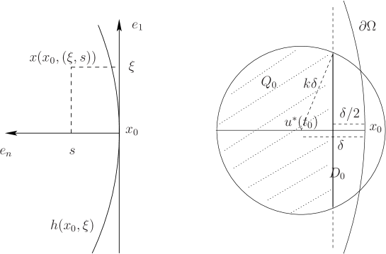
Figure 1: The coordinates $(\xi,s)$ and the domain $Q_{0}$ in Lemma 2.5.

If $j_{0}$ is sufficiently large, setting $t_{0}=\tau_{j_{0}}$ we have that $x_{0}=\pi(u^{*}(t_{0}))$ is well defined. Moreover $x_{0}\in\partial\Omega\cap B_{\frac{\bar{r}}{2}}(\bar{x})$ and

$$u^{*}(t_{0})=x_{0}+\delta e_{n}(x_{0}),\;\;\delta=|u^{*}(t_{0})-x_{0}|.$$

For $k=\frac{8}{3}\sqrt{2}$ let $Q_{0}$ be the set

$$Q_{0}=\{x(x_{0},(\xi,s)):|\xi|^{2}+(s-\delta)^{2}<k^{2}\delta^{2},\;s>{\delta}/{2}\}.$$

Since $\delta\rightarrow 0$ as $j_{0}\rightarrow+\infty$ we can assume that $\delta>0$ is so small ($\delta<\min\{\frac{1}{2Ck^{2}},\frac{r}{1+k}\}$ suffices) that $\overline{Q}_{0}\subset\Omega\cap B_{r}(x_{0})$.

Claim 1. $u^{*}(t)$ leaves $\overline{Q}_{0}$ through the disc $D_{0}={\partial Q_{0}\setminus\partial B_{k\delta}(u^{*}(t_{0}))}$.

From (2.4) we have $a_{0}\leq\mathcal{A}(v,(T_{-},T_{+}^{v}))$ for each $W^{1,2}$ map ${v:(T_{-},T_{+}^{v}]\rightarrow\mathbb{R}^{n}}$ that coincides with $u^{*}$ for $t\leq t_{0}$, and satisfies $v((t_{0},T_{+}^{v}))\subset\Omega$, $v(T_{+}^{v})\in\partial\Omega$ and (1.4). Therefore if we set

$$w(s)=x_{0}+se_{n}(x_{0}),$$

$s\in[0,\delta]$, we have

$$a_{0}\leq\mathcal{A}(u^{*},(T_{-},t_{0}))+\mathcal{J}(w,(0,\delta)).$$ (2.18)

On the other hand, if $u^{*}(t_{0}^{\prime})\in\partial Q_{0}(x_{0})\cap\partial B_{k\delta}(u^{*}(t_{0}))$, where

$$t_{0}^{\prime}=\sup\{t>t_{0}:u^{*}([t_{0},t))\subset\overline{Q}_{0}\setminus\partial B_{k\delta}(u^{*}(t_{0}))\},$$

from (2.7) it follows

$$\mathcal{A}(u^{*},(T_{-},t_{0}))+\mathcal{J}(u^{*},(t_{0},t_{0}^{\prime}))\leq a_{0}.$$ (2.19)

Using (2.17) we obtain

$$\mathcal{J}(w,(0,\delta))\leq\frac{4}{3}c^{\frac{1}{2}}\delta^{\frac{3}{2}},$$ (2.20)

and, since

$$c\frac{\delta}{4}\leq U(x(x_{0},(\xi,s))),\quad(\xi,s)\in\overline{Q}_{0}(x_{0}),$$

we also have, with $k$ defined above,

$$\frac{8}{3}c^{\frac{1}{2}}\delta^{\frac{3}{2}}=\frac{k}{\sqrt{2}}c^{\frac{1}{2}}\delta^{\frac{3}{2}}\leq\frac{c^{\frac{1}{2}}\delta^{\frac{1}{2}}}{\sqrt{2}}\int_{t_{0}}^{t_{0}^{\prime}}|\dot{u}^{*}(t)|dt\leq\sqrt{2}\int_{t_{0}}^{t_{0}^{\prime}}\sqrt{U(u^{*}(t))}|\dot{u}^{*}(t)|dt.$$ (2.21)

From (2.20) and (2.21) it follows

$$\mathcal{J}(w,(0,\delta))\leq\frac{1}{2}\mathcal{J}(u^{*},(t_{0},t_{0}^{\prime})),$$

and therefore (2.18) and (2.19) imply the absurd inequality $a_{0}<a_{0}$. This contradiction proves the claim.

From Claim 1 it follows that there is $t_{1}\in(t_{0},+\infty)$ with the following properties:

$$\begin{split}&u^{*}([t_{0},t_{1}))\subset Q_{0}(x_{0}),\\ &u(t_{1})\in D_{0}.\end{split}$$

Set $x_{0,1}=\pi(u^{*}(t_{1}))$ and $\delta_{1}=|u^{*}(t_{1})-x_{0,1}|$. Since $h(x_{0},0)=h_{\xi}(x_{0},0)=0$ and the radius $\rho_{\delta}=(k^{2}-\frac{1}{4})^{\frac{1}{2}}\delta$ of $D_{0}$ is proportional to $\delta$, we can assume that $\delta$ is so small that the ratio $\frac{2\delta_{1}}{\delta}$ and $\frac{|x_{0,1}-x_{0}|}{|u^{*}(t_{1})-x(x_{0},(0,\frac{\delta}{2}))|}$ are near $1$ so that we have

$$\begin{split}&\delta_{1}\leq\rho\delta,\;\;\text{for some}\;\;\rho<1,\\ &|x_{0,1}-x_{0}|\leq k\delta.\end{split}$$

We also have

$$t_{1}-t_{0}\leq k^{\prime}\delta^{\frac{1}{2}},\;\;k^{\prime}=\frac{8k}{c^{\frac{1}{2}}}.$$

This follows from

$$\begin{split}&(t_{1}-t_{0})\frac{c}{4}\delta\leq\mathcal{A}(u^{*},(t_{0},t_{1}))=\mathcal{J}(u^{*},(t_{0},t_{1}))\\ &=\sqrt{2}\int_{t_{0}}^{t_{1}}\sqrt{U(u^{*}(t))}|\dot{u^{*}}(t)|dt\leq 2\sqrt{c\delta}|u^{*}(t_{1})-u^{*}(t_{0})|\leq 2c^{\frac{1}{2}}k\delta^{\frac{3}{2}}.\end{split}$$

where we used (2.17) to estimate $\mathcal{J}$ on the segment joining $u^{*}(t_{0})$ with $u^{*}(t_{1})$.

We have $u^{*}(t_{1})=x_{0,1}+\delta_{1}e_{n}(x_{0,1})$ and we can apply Claim 1 to deduce that there exists $t_{2}>t_{1}$ such that

$$\begin{split}&u^{*}([t_{1},t_{2}))\subset Q_{1}(x_{0,1}),\\ &u^{*}(t_{2})\in D_{1},\end{split}$$

where $Q_{1}$ and $D_{1}$ are defined as $Q_{0}$ and $D_{0}$ with $\delta_{1}$ and $x(x_{0,1},(\xi,s))$ instead of $\delta$ and $x(x_{0},(\xi,s))$. Therefore an induction argument yields sequences $\{t_{j}\}$, $\{x_{0,j}\}$, $\{\delta_{j}\}$ and $\{Q_{j}(x_{0,j})\}$ such that

$$\begin{split}&u^{*}([t_{j},t_{j+1}))\subset Q_{j}(x_{0,j}),\quad x_{0,j}=\pi(u^{*}(t_{j})),\\ &\delta_{j+1}\leq\rho\delta_{j}\leq\rho^{j+1}\delta,\\ &|x_{0,j+1}-x_{0,j}|\leq k\delta_{j}\leq k\rho^{j}\delta,\\ &(t_{j+1}-t_{j})\leq k^{\prime}\delta_{j}^{1/2}\leq k^{\prime}\rho^{j/2}\delta^{1/2},\\ &u^{*}(t_{j})=x_{0,j}+\delta_{j}e_{n}(x_{0,j})\in D_{j}.\end{split}$$ (2.22)

We can also assume that $Q_{j}(x_{0,j})\subset\Omega\cap B_{r}(x_{0})$, for all $j\in\mathbb{N}$. This follows from $|u^{*}(t_{j+1})-u^{*}(t_{j})|\leq k\delta_{j}\leq k\rho^{j}\delta$.

From (2.22) we obtain that there exists $T$ with $t_{0}<T\leq\frac{k^{\prime}\delta^{\frac{1}{2}}}{1-\rho^{\frac{1}{2}}}$ such that

$$\begin{split}&u^{*}(T)=\lim_{t\rightarrow T}u^{*}(t)=\lim_{j\rightarrow+\infty}x_{0,j}\in\partial\Omega\setminus P,\\ &|u^{*}(T)-x_{0}|\leq\frac{k\delta}{1-\rho}.\end{split}$$

This contradicts the existence of the sequence $\{\tau_{j}\}$, with $\lim_{j\to\infty}\tau_{j}=+\infty$, appearing in (2.16) and establishes (2.15). The proof of the lemma is complete. ∎

We continue by showing (2.15) contradicts (2.8).

Lemma 2.6.

Assume that $\Gamma_{+}$ has positive diameter. Then

$$T_{+}<+\infty.$$

An analogous statement applies to $\Gamma_{-}$ and $T_{-}$.

Proof.

From Lemma 2.5, if $T_{+}=+\infty$ there exists $p\in P$ such that $\lim_{t\to+\infty}u^{*}(t)=p$. We use a local argument to show that this is impossible if $\Gamma_{+}$ has positive diameter. By a suitable change of variable we can assume that $p=0$ and that, in a neighborhood of $0\in\mathbb{R}^{n}$, $U$ reads

$$U(u)=V(u)+W(u),$$

where $V$ is the quadratic part of $U$:

$$V(u)=\frac{1}{2}\Bigl{(}-\sum_{i=1}^{m}\lambda_{i}^{2}u_{i}^{2}+\sum_{i=m+1}^{n}\lambda_{i}^{2}u_{i}^{2}\Bigr{)},\qquad\lambda_{i}>0$$ (2.23)

and $W$ satisfies,

$$|W(u)|\leq C|u|^{3},\quad|W_{x}(u)|\leq C|u|^{2},\quad|W_{xx}(u)|\leq C|u|.$$ (2.24)

Consider the Hamiltonian system with

$$H(p,q)=\frac{1}{2}|p|^{2}-U(q),\quad p\in\mathbb{R}^{n},\ q\in\Omega\subset\mathbb{R}^{n}.$$

For this system the origin of $\mathbb{R}^{2n}$ is an equilibrium point that corresponds to the critical point $p=0$ of $U$. Set $D=\text{diag}(-\lambda_{1}^{2},\ldots,-\lambda_{m}^{2},\lambda_{m+1}^{2},\ldots,\lambda_{n}^{2})$. The eigenvalues of the symplectic matrix

$$\left(\begin{array}[]{cc}0&D\\ I&0\end{array}\right)$$

are

$$\begin{split}&-\lambda_{i},\;\;i=m+1,\ldots,n\\ &\phantom{-\;\,}\lambda_{i},\;\;i=m+1,\ldots,n\\ &\pm i\lambda_{i},\;\;i=1,\ldots,m.\end{split}$$

Let $(e_{1},0),\ldots,(e_{n},0)$, $(0,e_{1}),\ldots,(0,e_{n})$ be the basis of $\mathbb{R}^{2n}$ defined by $e_{j}=(\delta_{j1},\ldots,\delta_{jn})$, where $\delta_{ji}$ is Kronecker’s delta. The stable $S^{s}$, unstable $S^{u}$ and center $S^{c}$ subspaces invariant under the flow of the linearized Hamiltonian system at $0\in\mathbb{R}^{2n}$ are

$$\begin{split}&S^{s}=\text{span}\{(-\lambda_{j}e_{j},e_{j})\}_{j=m+1}^{n},\\ &S^{u}=\text{span}\{(\lambda_{j}e_{j},e_{j})\}_{j=m+1}^{n},\\ &S^{c}=\text{span}\{(e_{j},0),(0,e_{j})\}_{j=1}^{m}.\end{split}$$

From (2.15) and (1.4) we have

$$\lim_{t\rightarrow+\infty}(\dot{u}^{*}(t),u^{*}(t))=0\in\mathbb{R}^{2n}.$$

Let $W^{s}$ and $W^{u}$ be the local stable and unstable manifold and let $W^{c}$ be a local center manifold at $0\in\mathbb{R}^{2n}$. From the center manifold theorem [4], [10], there is a constant $\lambda_{0}>0$ such that, for each solution $(p(t),q(t))$ that remains in a neighborhood of $0\in\mathbb{R}^{2n}$ for positive time, there is a solution $(p^{c}(t),q^{c}(t))\in W^{c}$ that satisfies

$$|(p(t),q(t))-(p^{c}(t),q^{c}(t))|=\text{O}(e^{-\lambda_{0}t}).$$ (2.25)

Since $W^{c}$ is tangent to $S^{c}$ at $0\in\mathbb{R}^{2n}$, the projection $W_{0}^{c}$ on the configuration space is tangent to $S_{0}^{c}=\text{span}\{e_{j}\}_{j=1}^{m}$, which is the projection of $S^{c}$ on the configuration space. Therefore, if $(p^{c},q^{c})\not\equiv 0$, given $\gamma>0$, by (2.25) there is $t_{\gamma}$ such that $d(q(t),S_{0}^{c})\leq\gamma|q(t)|$, for $t\geq t_{\gamma}$. For $\gamma$ small, this implies that $q(t)\not\in\Omega$ for $t\geq t_{\gamma}$. It follows that $(p^{c},q^{c})\equiv 0$ and from (2.25) $(p(t),q(t))$ converges to zero exponentially. This is possible only if $(p(t),q(t))\in W^{s}$ and, in turn, only if $q(t)\in W_{0}^{s}$, the projection of $W^{s}$ on the configuration space. This argument leads to the conclusion that the trajectory of $u^{*}$ in a neighborhood of $0$ is of the form

$$u^{*}(t(s))=\mathfrak{u}^{*}(s)=s\eta+z(s),$$ (2.26)

where

$$\eta=\sum_{i=m+1}^{n}\eta_{i}e_{i}$$

is a unit vector, $s\in[0,s_{0})$ for some $s_{0}>0$, and $z(s)$ satisfies

$$z(s)\cdot\eta=0,\quad|z(s)|\leq c|s|^{2},\quad|z^{\prime}(s)|\leq c|s|$$ (2.27)

for a positive constant $c$.

We are now in the position of constructing our local perturbation of $u$. We first discuss the case $U=V$, $z(s)=0$. We set

$$\bar{u}(s)=s\eta$$

and, in some interval $[1,s_{1}]$, construct a competing map $\bar{v}:[1,s_{1}]\rightarrow\mathbb{R}^{n}$,

$$\bar{v}=\bar{u}+ge_{1},\quad g:[1,s_{1}]\rightarrow\mathbb{R},$$

with the following properties:

$$V(\bar{v}(1))=0,$$

$$\bar{v}(s_{1})=\bar{u}(s_{1}),$$

$$\mathcal{J}_{V}(\bar{v},[1,s_{1}])<\mathcal{J}_{V}(\bar{u},[0,s_{1}]).$$ (2.28)

The basic observation is that, if we move from $\bar{u}$ in the direction of one of the eigenvectors $e_{1},\ldots,e_{m}$ corresponding to negative eigenvalues of the Hessian of $V$, the potential $V$ decreases and therefore, for each $s_{0}\in(1,s_{1})$ we can define the function $g$ in the interval $[1,s_{0}]$ so that

$$\mathcal{J}_{V}(\bar{u}+ge_{1},(1,s_{0}))=\mathcal{J}_{V}(\bar{u},(1,s_{0})).$$ (2.29)

Indeed it suffices to impose that $g:(1,s_{0}]\rightarrow\mathbb{R}$ satisfies the condition

$$\sqrt{V(\bar{u}(s))}=\sqrt{1+g^{\prime 2}(s)}\sqrt{V(\bar{u}(s)+g(s)e_{1})},\;\;s\in(1,s_{0}].$$

According with this condition we take $g$ as the solution of the problem

$$\left\{\begin{array}[]{l}{g}^{\prime}=\displaystyle-\frac{\lambda_{1}g}{\sqrt{s^{2}\lambda_{\eta}^{2}-\lambda_{1}^{2}g^{2}}}=-\frac{\frac{\lambda_{1}g}{s\lambda_{\eta}}}{\sqrt{1-\frac{\lambda_{1}^{2}g^{2}}{s^{2}\lambda_{\eta}^{2}}}}\\ g(1)=\frac{\lambda_{\eta}}{\lambda_{1}}\end{array}\right.,$$ (2.30)

where we have used (2.23) and set

$$\lambda_{\eta}=\sqrt{\sum_{i=m+1}^{n}\lambda_{i}^{2}\eta_{i}^{2}}.$$

Note that the initial condition in (2.30) implies $V(\bar{v}(1))=0$. The solution $g$ of (2.30) is well defined in spite of the fact that the right hand side tends to $-\infty$ as $s\rightarrow 1$. Since $g$ defined by (2.30) is positive for $s\in[1,+\infty)$, to satisfy the condition $\bar{v}(s_{1})=\bar{u}(s_{1})$, we give a suitable definition of $g$ in the interval $[s_{0},s_{1}]$ in order that $g(s_{1})=0$. Choose a number $\alpha\in(0,1)$ and extend $g$ with continuity to the interval $[s_{0},s_{1}]$ by imposing that

$$\sqrt{V(\bar{u}(s))}=\alpha\sqrt{1+g^{\prime 2}(s)}\sqrt{V(\bar{u}(s)+g(s)e_{1})},\;\;s\in(s_{0},s_{1}].$$ (2.31)

Therefore, in the interval $(s_{0},s_{1}]$, we define $g$ by

$${g}^{\prime}=-\frac{1}{\alpha}\sqrt{\frac{1-\alpha^{2}+\alpha^{2}\frac{\lambda_{1}^{2}g^{2}}{s^{2}\lambda_{\eta}^{2}}}{1-\frac{\lambda_{1}^{2}g^{2}}{s^{2}\lambda_{\eta}^{2}}}}\leq-\frac{\sqrt{1-\alpha^{2}}}{\alpha}.$$ (2.32)

Figure 2: The maps $\bar{u}(s)$ and $\bar{v}(s)$.

Since (2.31) implies

$$\mathcal{J}_{V}(\bar{v},[s_{0},s_{1}])=\frac{1}{\alpha}\mathcal{J}_{V}(\bar{u},[s_{0},s_{1}]),$$

from (2.29) we see that $\bar{v}$ satisfies also the requirement (2.28) above if we can choose $\alpha\in(0,1)$ and $1<s_{0}<s_{1}$ in such a way that

$$\mathcal{J}_{V}(\bar{u},(0,1))>\frac{1-\alpha}{\alpha}\mathcal{J}_{V}(\bar{u},(s_{0},s_{1})).$$

Since (2.32) implies $s_{1}<s_{0}+\frac{\alpha g(s_{0})}{\sqrt{1-\alpha^{2}}}$ a sufficient condition for this is

$$\mathcal{J}_{V}(\bar{u},(0,1))>\frac{1-\alpha}{\alpha}\mathcal{J}_{V}\Bigl{(}\bar{u},\Bigl{(}s_{0},s_{0}+\frac{\alpha g(s_{0})}{\sqrt{1-\alpha^{2}}}\Bigr{)}\Bigr{)},$$

or equivalently

$$1>\frac{1-\alpha}{\alpha}\Big{(}\Bigl{(}s_{0}+\frac{\alpha g(s_{0})}{\sqrt{1-\alpha^{2}}}\Bigr{)}^{2}-s_{0}^{2}\Big{)}=2s_{0}g(s_{0})\sqrt{\frac{1-\alpha}{1+\alpha}}+\frac{\alpha g^{2}(s_{0})}{1+\alpha}.$$ (2.33)

By a proper choice of $s_{0}$ and $\alpha$ the right hand side of (2.33) can be made as small as we like. For instance we can fix $s_{0}$ so that $g(s_{0})\leq\frac{1}{4}$ and then choose $\alpha$ in such a way that $\frac{1}{2}s_{0}\sqrt{\frac{1-\alpha}{1+\alpha}}\leq\frac{1}{4}$ and conclude that (2.28) holds.

Next we use the function $g$ to define a comparison map $v$ that coincides with $u^{*}$ outside an $\epsilon$-neighborhood of $0$ and show that the assumption that the trajectory of $u^{*}$ ends up in some $p\in P$ must be rejected. For small $\epsilon>0$ we define

$$v(\epsilon s)=\epsilon s\eta+z(\epsilon s)+\epsilon g(s-\sigma)e_{1},\;\;s\in[1+\sigma,s_{1}+\sigma],$$ (2.34)

where $\sigma=\sigma(\epsilon)$ is determined by the condition

$$U(v(\epsilon(1+\sigma)))=0,$$

which, using (2.23), (2.24), (2.27) and $g(1)=\frac{\lambda_{\eta}}{\lambda_{1}}$, after dividing by $\epsilon^{2}$, becomes

$$\frac{1}{2}\lambda_{\eta}^{2}((1+\sigma)^{2}-1)=\epsilon f(\sigma,\epsilon),$$ (2.35)

where $f(\sigma,\epsilon)$ is a smooth bounded function defined in a neighborhood of $(0,0)$. For small $\epsilon>0$, there is a unique solution $\sigma(\epsilon)=\text{O}(\epsilon)$ of (2.35). Note also that (2.34) implies that

$$v(\epsilon(s_{1}+\sigma))=\mathfrak{u}^{*}(\epsilon(s_{1}+\sigma)).$$

We now conclude by showing that, for $\epsilon>0$ small, it results

$$\mathcal{J}_{U}(\mathfrak{u}^{*}(\epsilon\cdot),(0,s_{1}+\sigma))>\mathcal{J}_{U}(v(\epsilon\cdot),(1+\sigma,s_{1}+\sigma)).$$ (2.36)

From (2.26) and (2.34) we have

$$\lim_{\epsilon\rightarrow 0^{+}}\epsilon^{-1}\Bigl{|}\frac{d}{ds}\mathfrak{u}^{*}(\epsilon s)\Bigr{|}=1,\;\;\;\lim_{\epsilon\rightarrow 0^{+}}\epsilon^{-1}\Bigl{|}\frac{d}{ds}v(\epsilon s)\Bigr{|}=\sqrt{1+g^{\prime 2}(s)},$$ (2.37)

and, using also (2.24) and $\sigma=\text{O}(\epsilon)$,

$$\begin{split}&\lim_{\epsilon\rightarrow 0^{+}}\epsilon^{-2}U(\mathfrak{u}^{*}(\epsilon s))=V(\bar{u}(s)),\;\;s\in(0,s_{1}),\\ &\lim_{\epsilon\rightarrow 0^{+}}\epsilon^{-2}U(v(\epsilon s))=V(\bar{v}(s)),\;\;s\in(1,s_{1})\end{split}$$ (2.38)

uniformly in compact intervals.

The limits (2.37) and (2.38) imply

$$\begin{split}&\lim_{\epsilon\rightarrow 0^{+}}\epsilon^{-2}\mathcal{J}_{U}(\mathfrak{u}^{*}(\epsilon\cdot),(0,s_{1}+\sigma))=\lim_{\epsilon\rightarrow 0^{+}}\sqrt{2}\int_{0}^{s_{1}+\sigma}\sqrt{\epsilon^{-2}U(\mathfrak{u}^{*}(\epsilon s))}\epsilon^{-1}\Bigl{|}\frac{d}{ds}\mathfrak{u}^{*}(\epsilon s)\Bigr{|}ds,\\ &=\sqrt{2}\int_{0}^{s_{1}}\sqrt{V(\bar{u}(s))}ds=\mathcal{J}_{V}(\bar{u},(0,s_{1}))\\ &\lim_{\epsilon\rightarrow 0^{+}}\epsilon^{-2}\mathcal{J}_{U}(v(\epsilon\cdot),(1+\sigma,s_{1}+\sigma))=\lim_{\epsilon\rightarrow 0^{+}}\sqrt{2}\int_{1+\sigma}^{s_{1}+\sigma}\sqrt{\epsilon^{-2}U(v(\epsilon s))}\epsilon^{-1}\Bigl{|}\frac{d}{ds}v(\epsilon s)\Bigr{|}ds,\\ &=\sqrt{2}\int_{1}^{s_{1}}\sqrt{V(\bar{v}(s))}\sqrt{1+g^{\prime 2}(s)}ds=\mathcal{J}_{V}(\bar{v},(1,s_{1})).\end{split}$$

This and (iii) above imply that, indeed, the inequality (2.36) holds for small $\epsilon>0$. The proof is complete. ∎

We can now complete the proof of Theorem 1.1. We show that the map $u^{*}:(T_{-},T_{+})\rightarrow\mathbb{R}^{n}$ possesses all the required properties. The fact that $u^{*}$ satisfies (1.2) and (1.4) follows from Lemma 2.3. Lemma 2.2 implies (1.5) and, if $T_{-}>-\infty$, also (1.6). The fact that $x_{-}\in\Gamma_{-}\setminus P$ is a consequence of Lemma 2.4 and implies that $\Gamma_{-}$ has positive diameter. Viceversa, if $\Gamma_{-}$ has positive diameter, Lemmas 2.5 and 2.6 imply that $T_{-}>-\infty$ and that (1.6) holds for some $x_{-}\in\Gamma_{-}\setminus P$. The proof of Theorem 1.1 is complete.

Remark.

From Theorem 1.1 it follows that if $N$ is even then there are at least $N/2$ distinct orbits connecting different elements of $\{\Gamma_{1},\ldots,\Gamma_{N}\}$. If $N$ is odd there are at least $(N+1)/2$. Simple examples show that, given distinct $\Gamma_{i},\Gamma_{j}\in\{\Gamma_{1},\ldots,\Gamma_{N}\}$, an orbit connecting them does not always exist. Let

$$\mathcal{U}_{ij}=\{u\in W^{1,2}((T_{-}^{u},T_{+}^{u});\mathbb{R}^{n}):u((T_{-}^{u},T_{+}^{u}))\subset\Omega,u(T_{-}^{u})\in\Gamma_{i},u(T_{+}^{u})\in\Gamma_{j}\}$$

with $i\neq j$ and

$$d_{ij}=\inf_{u\in\mathcal{U}_{ij}}\mathcal{A}(u,(T_{-}^{u},T_{+}^{u})).$$

An orbit connecting $\Gamma_{i}$ and $\Gamma_{j}$ exists if

$$d_{ij}<d_{ik}+d_{kj},\quad\forall k\neq i,j.$$

The proof of Theorem 1.2 uses, with obvious modifications, the same arguments as in the proof of Theorem 1.1 to characterize $u^{*}$ as the limit of a minimizing sequence $\{u_{j}\}$ of the action functional

$$\mathcal{A}(u,(0,T^{u}))=\int_{0}^{T^{u}}\Bigl{(}\frac{1}{2}|\dot{u}(t)|^{2}+U(u(t))\Bigr{)}dt.$$ (2.39)

in the set

$$\mathcal{U}=\{u\in W^{1,2}((0,T^{u});\mathbb{R}^{n}):0<T_{+}^{u}<+\infty,\ u(0)=0,\ u([0,T_{+}^{u}))\subset\Omega,\ u(T_{+}^{u})\in\partial\Omega\}.$$ (2.40)

Remark.

In the symmetric case of Theorem 1.2 it is easy to construct an example with $T_{+}<T_{+}^{\infty}$. For $U(x)=1-|x|^{2}$, $x\in\mathbb{R}^{2}$, the solution $u:[0,{\pi}/{2}]\rightarrow\mathbb{R}^{2}$ of (1.2) determined by (1.4) and $u([0,{\pi}/{2}])=\{(s,0):s\in[0,1]\}$ is a minimizer of $\mathcal{A}$ in $\mathcal{U}$. For $\epsilon$ small, let $t_{\epsilon}=\arcsin(1-\epsilon)$ and define $u_{\epsilon}:[0,T^{u_{\epsilon}}]\rightarrow\mathbb{R}^{2}$ as the map determined by (1.4), $u_{\epsilon}([0,t_{\epsilon}])=\{(s,0):s\in[0,1-\epsilon)\}$ and $u_{\epsilon}((t_{\epsilon},T^{u_{\epsilon}}])=\{(1-\epsilon,s):s\in(0,\sqrt{2\epsilon-\epsilon^{2}}]\}$. In this case $T_{+}={\pi}/{2}$ and $T_{+}^{\infty}=3\pi/4$.

2.1 On the existence of heteroclinic connections

Corollary 1.3 states the existence of heteroclinic connections under the assumptions of Theorem 1.1 and, in particular, that $U\in C^{2}$. Actually, by examining the proof of Theorem 1.1 we can establish an existence result under weaker hypotheses. In the special case $\partial\Omega=P$, $\#P\geq 2$, given $p_{-}\in P$, the set $\mathcal{U}$ defined in (2.1) takes the form

$$\begin{split}\mathcal{U}=\bigl{\{}u\in W^{1,2}((T_{-}^{u},T_{+}^{u});\mathbb{R}^{n}):{-\infty<T_{-}^{u}<T_{+}^{u}<+\infty,}\hskip 62.59596pt\\ u((T_{-}^{u},T_{+}^{u}))\subset\Omega,\ U(u(0))=U_{0},\ u(T_{-}^{u})=p_{-},\ u(T_{+}^{u})\in P\setminus\{p_{-}\}\}.\end{split}$$

In this section we slightly enlarge the set $\mathcal{U}$ by allowing $T_{\pm}^{u}=\pm\infty$ and consider the admissible set

$$\begin{split}\widetilde{\mathcal{U}}=\bigl{\{}u\in W^{1,2}_{loc}((T_{-}^{u},T_{+}^{u});\mathbb{R}^{n}):{-\infty\leq T_{-}^{u}<T_{+}^{u}\leq+\infty,}\hskip 62.59596pt\\ u((T_{-}^{u},T_{+}^{u}))\subset\Omega,\ U(u(0))=U_{0},\ \lim_{t\rightarrow T_{-}^{u}}u(t)=p_{-},\ \lim_{t\rightarrow T_{+}^{u}}u(t)\in P\setminus\{p_{-}\}\}.\end{split}$$

Proposition 2.7.

Assume that $U$ is a non-negative continuous function, which vanishes in a finite set $P$, $\#P\geq 2$, and satisfies

$$\sqrt{U(x)}\geq\sigma(|x|),\;\;x\in\Omega,\;\;|x|\geq r_{0}$$

for some $r_{0}>0$ and a non-negative function $\sigma:[r_{0},+\infty)\rightarrow\mathbb{R}$ such that $\int_{r_{0}}^{+\infty}\sigma(r)dr=+\infty$.

Given $p_{-}\in P$ there is $p_{+}\in P\setminus\{p_{-}\}$ and a Lipschitz-continuous map $u^{*}:(T_{-},T_{+})\rightarrow\Omega$ that satisfies (1.4) almost everywhere on $(T_{-},T_{+})$,

$$\lim_{t\rightarrow T_{\pm}}u^{*}(t)=p_{\pm},$$

and minimizes the action functional $\mathcal{A}$ on $\tilde{\mathcal{U}}$.

Proof.

We begin by showing that

$$a_{0}=\inf_{u\in\mathcal{U}}\mathcal{A}=\inf_{u\in\tilde{\mathcal{U}}}\mathcal{A}=\tilde{a}_{0}.$$ (2.41)

Since $\mathcal{U}\subset\tilde{\mathcal{U}}$ we have $a_{0}\geq\tilde{a}_{0}$. On the other hand arguing as in the proof of Lemma 2.2, if $T_{+}-T_{-}=+\infty$, given a small number $\epsilon>0$, we can construct a map $u_{\epsilon}\in\mathcal{U}$ that satisfies

$$a_{0}\leq\mathcal{A}(u_{\epsilon},(T_{-}^{u_{\epsilon}},T_{+}^{u_{\epsilon}}))\leq\mathcal{A}(u,(T_{-}^{u},T_{+}^{u}))+\eta_{\epsilon}$$

where $\eta_{\epsilon}\rightarrow 0$ as $\epsilon\rightarrow 0$. This implies $a_{0}\leq\tilde{a}_{0}$ and establishes (2.41). It follows that we can proceed as in the proof of Theorem 1.1 and define $u^{*}\in\tilde{\mathcal{U}}$ as the limit of a minimizing sequence $\{u_{j}\}\subset\mathcal{U}$. The arguments in the proof of Lemma 2.2 show that (2.8) holds. It remain to show that $u^{*}$ is Lipschitz-continuous. Looking at the proof of Lemma 2.3 we see that the continuity of $U$ is sufficient for establishing that (1.4) holds almost everywhere on $(T_{-},T_{+})$, and the Lipschitz character of $u^{*}$ follows. The proof is complete. ∎

Remark.

Without further information on the behavior of $U$ in a neighborhood of $p_{\pm}$ nothing can be said on $T_{\pm}$ being finite or infinite and it is easy to construct examples to show that all possible combinations are possible. As shown in Lemma 2.4 a sufficient condition for $T_{\pm}=\pm\infty$ is that, in a neighborhood of $p=p_{\pm}$, $U(x)$ is bounded by a function of the form $c|x-p|^{2}$, $c>0$. $U$ of class $C^{1}$ is a sufficient condition in order that $u^{*}$ is of class $C^{2}$ and satisfies (1.2).

3 Examples

In this section we show a few simple applications of Theorems 1.1 and 1.2.

Our first application describes a class of potentials with the property that, in spite of the existence of possibly infinitely many critical values, (1.2) has a nontrivial periodic orbit on any energy level.

Proposition 3.1.

Assume that $U:\mathbb{R}^{n}\rightarrow\mathbb{R}$ satisfies

$$\begin{split}&U(-x)=U(x),\;\;x\in\mathbb{R}^{n},\\ &U(0)=0,\ U(x)<0\ \mbox{for}\ x\neq 0,\\ &\lim_{|x|\to\infty}U(x)=-\infty\end{split}$$

Assume moreover that each non zero critical point of $U$ is hyperbolic with Morse index $i_{m}\geq 1$. Then there is a nontrivial periodic orbit of (1.2) on the energy level $\frac{1}{2}|\dot{u}|^{2}-U(u)=\alpha$ for each $\alpha>0$.

Proof.

For each $\alpha>0$ we set $\tilde{U}=U(x)+\alpha$ and let $\Omega\subset\{\tilde{U}>0\}$ be the connected component that contains the origin. $\Omega$ is open, nonempty and bounded and, from the assumptions on the properties of the critical points of $U$, it follows that $\partial\Omega$ is connected and contains at most a finite number of critical points. Therefore we are under the assumptions of Corollary 1.6 for the case $N=1$ and the existence of the periodic orbit follows. ∎

An example of potential $U:\mathbb{R}^{2}\rightarrow\mathbb{R}$ that satisfies the assumptions in Proposition 3.1 is, in polar coordinates $r,\theta$,

$$U(r,\theta)=-r^{2}+\frac{1}{2}\tanh^{4}(r)\cos^{2}(r^{-1})\cos^{2k}(2\theta),$$

where $k>0$ is a sufficiently large number.

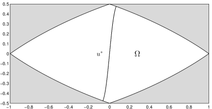
Figure 3: Symmetric periodic orbit for the example with potential (3.1).

Next we give another application of Corollary 1.6. For the potential $U:\mathbb{R}^{2}\rightarrow\mathbb{R}$, with

$$U(x)=\frac{1}{2}(1-x_{1}^{2})^{2}+\frac{1}{2}(1-4x_{2}^{2})^{2},$$ (3.1)

the energy level $\alpha=-\frac{1}{2}$ is critical and corresponds to four hyperbolic critical points $p_{1}=(1,0)$, $-p_{1}$, $p_{2}=(0,\frac{1}{2})$ and $-p_{2}$. The connected component $\Omega\subset\{\tilde{U}>0\}$, ($\tilde{U}=U(x)-\frac{1}{2}$) that contains the origin is bounded by a simple curve $\Gamma$ that contains $\pm p_{1}$ and $\pm p_{2}$. In spite of the presence of these critical points, from Theorem 1.2 it follows that there is a minimizer $u\in\mathcal{U}$, with $\mathcal{U}$ as in (2.40) and $u(T^{u})\in\Gamma\setminus\{\pm p_{1},\pm p_{2}\}$, and Corollary 1.6 implies the existence of a periodic solution $v^{*}$. Note that there are also two heteroclinic orbits, solutions of (1.2) and (1.4):

$$u_{1}(t)=(\tanh(t),0),\qquad u_{2}(t)=(0,\frac{1}{2}\tanh(2t)).$$

These orbits connect $p_{j}$ to $-p_{j}$, for $j=1,2$. By Theorem 1.2 both $u_{1}$ and $u_{2}$ have action greater than $v^{*}|_{(-T_{+},T_{+})}$.

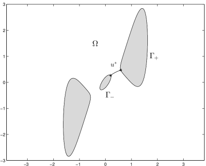
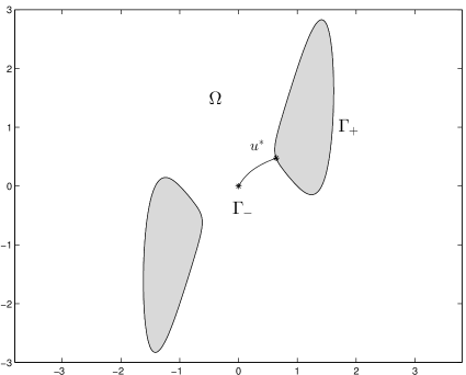
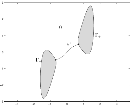
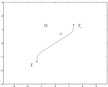
Figure 4: Bifurcations of dynamics of (1.2) with the $\alpha=0$, bottom left: $\alpha=0.05$, bottom right: $\alpha=-U(p_{2},1)$. The shaded regions are not accessible.

Our last example shows that Theorems 1.1 and 1.2 can be used to derive information on the rich dynamics that (1.2) can exhibit when $U$ undergoes a small perturbation. We consider a family of potentials $U:\mathbb{R}^{2}\times[0,1]\rightarrow\mathbb{R}$. We assume that $U(x,0)=x_{1}^{6}+x_{2}^{2}$ which from various points of view is a structurally unstable potential and, for $\lambda>0$ small, we consider the perturbed potential

$$U(x,\lambda)=2\lambda^{4}x_{1}^{2}+x_{2}^{2}-2\lambda^{2}x_{1}x_{2}-3\lambda^{2}x_{1}^{4}+x_{1}^{6}.$$ (3.2)

This potential satisfies $U(-x,\lambda)=U(x,\lambda)$ and, for $\lambda>0$, has the five critical points $p_{0},\pm p_{1}$ and $\pm p_{2}$ defined by

$$p_{0}=(0,0),$$

$$p_{1}=(\lambda(1-(\frac{2}{3})^{\frac{1}{2}})^{\frac{1}{2}},\lambda^{3}(1-(\frac{2}{3})^{\frac{1}{2}})^{\frac{1}{2}}),$$

$$p_{2}=(\lambda(1+(\frac{2}{3})^{\frac{1}{2}})^{\frac{1}{2}},\lambda^{3}(1+(\frac{2}{3})^{\frac{1}{2}})^{\frac{1}{2}}),$$

which are all hyperbolic.

We have $U(p_{2},\lambda)<0=U(p_{0},\lambda)<U(p_{1},\lambda)$ and $p_{0}$ is a local minimum, $p_{1}$ a saddle and $p_{2}$ a global minimum. Let $\alpha$ be the energy level. For $-\alpha<U(p_{2},\lambda)$ or $-\alpha\geq U(p_{1},\lambda)$ no information can be derived from Theorems 1.1 and 1.2 therefore we assume $-\alpha\in[U(p_{2},\lambda),U(p_{1},\lambda))$. For $-\alpha=U(p_{2},\lambda)$ Corollary 1.3 or Corollary 1.6 yields the existence of a heteroclinic connection $u_{2}$ between $-p_{2}$ and $p_{2}$. For $-\alpha\in(U(p_{2},\lambda),0)$ Corollary 1.6 implies the existence of a periodic orbit $u_{\alpha}$. This periodic orbit converges uniformly in compact intervals to $u_{2}$ and the period $T_{\alpha}\rightarrow+\infty$ as $-\alpha\rightarrow U(p_{2},\lambda)^{+}$. For $\alpha=0$ Corollary 1.4 implies the existence of two orbits $u_{0}$ and $-u_{0}$ homoclinic to $p_{0}=0$. We can assume that $u_{0}$ satisfies the condition $u_{0}(-t)=u_{0}(t)$ and that $u_{\alpha}(0)=0$. Then we have that $u_{\alpha}(\cdot\pm\frac{T_{\alpha}}{4})$ converges uniformly in compact intervals to $\mp u_{0}$ and $T_{\alpha}\rightarrow+\infty$ as $-\alpha\rightarrow 0^{-}$. For $-\alpha\in(0,U(p_{1},\lambda))$, $\partial\Omega$ is the union of three simple curves all of positive diameter: $\Gamma_{0}$ that includes the origin and $\pm\Gamma_{2}$ which includes $\pm p_{2}$ and Corollary 1.5 together with the fact that $U(\cdot,\lambda)$ is symmetric imply the existence of two periodic solutions $\tilde{u}_{\alpha}$ and $-\tilde{u}_{\alpha}$ with $\tilde{u}_{\alpha}$ that oscillates between $\Gamma_{0}$ and $\Gamma_{2}$ in each time interval equal to $\frac{T_{\alpha}}{2}$. Assuming that $\tilde{u}_{\alpha}(0)\in\Gamma_{2}$ we have that, as $-\alpha\rightarrow 0^{+}$, $\tilde{u}_{\alpha}\rightarrow u_{0}$ uniformly in compacts and $T_{\alpha}\rightarrow+\infty$. Finally we observe that, in the limit $-\alpha\rightarrow U(p_{1},\lambda)^{-}$, $\tilde{u}_{\alpha}$ converges uniformly in $\mathbb{R}$ to the constant solution $u\equiv p_{1}$.

Acknowledgements

The first author is indebted with Peter Bates for fruitful discussions on the subject of this paper.

References

[1] N. Alikakos and G. Fusco.
On the connection
problem for potentials with several global minima.
Indiana Univ. Math. Journ.57 No. 4, 1871-1906 (2008)
[2] P. Antonopoulos and P. Smyrnelis.
On minimizers
of the Hamiltonian system , and on the existence of
heteroclinic, homoclinic and periodic connections.
Preprint (2016)
[3] A. Braides.
Approximation of
Free-Discontinuity Problems. Lectures Notes in Mathematics 1694,
Springer-Verlag, Heidelberg (1998)
[4] A. Bressan.
Tutorial on the Center Manifold
Theorem. Hyperbolic systems of balance laws. CIME course (Cetraro
2003). Springer Lecture Notes in Mathematics 1911,
327-344. Springer-Verlag, Heidelberg (2007)
[5] G. Buttazzo, M. Giaquinta, S. Hildebrandt.
One-dimensional Calculus of Variations: an Introduction
Oxford University Press, Oxford (1998)
[6] N. V. De Paulo and P. A. S. Salomo.
Systems of transversal sections near critical energy
levels of Hamiltonian systems in , arXiv:1310.8464v2 (2016)
[7] A. Monteil and F. Santambrogio.
Metric
methods for heteroclinic connections. Mathematical Methods in the
Applied Sciences,
DOI: 10.1002/mma.4072 (2016)
[8] C. Sourdis.
The heteroclinic connection
problem for general double-well potentials.
Mediterranean Journal of Mathematics13 No. 6,
4693-4710 (2016)
[9] P. Sternberg.
Vector-Valued Local
Minimizers of Nonconvex Variational Problems, Rocky Mountain
J. Math.21 No. 2, 799-807 (1991)
[10] A. Vanderbauwhede.
Centre manifolds, normal
forms and elementary bifurcations.
Dynamics
Reported2 No. 4, 89-169 (1989)
[11] A. Zuniga and P. Sternberg.
On the
heteroclinic connection problem for multi-well gradient systems.
Journal of Differential Equations261 No. 7,
3987-4007 (2016)