Non-Stoquastic Interactions in Quantum Annealing via the Aharonov-Anandan Phase

Abstract

We argue that a complete description of quantum annealing (QA) implemented with continuous variables must take into account the non-adiabatic Aharonov-Anandan geometric phase that arises when the system Hamiltonian changes during the anneal. We show that this geometric effect leads to the appearance of non-stoquastic terms in the effective quantum Ising Hamiltonians that are typically used to describe QA with flux-qubits. We explicitly demonstrate the effect of these geometric interactions when QA is performed with a system of one and two coupled flux-qubits. The realization of non-stoquastic Hamiltonians has important implications from a computational complexity perspective, since it is believed that in many cases QA with stoquastic Hamiltonians can be efficiently simulated via classical algorithms such as Quantum Monte Carlo. It is well-known that the direct implementation of non-stoquastic interactions with flux-qubits is particularly challenging. Our results suggest an alternative path for the implementation of non-stoquastic interactions via geometric phases that can be exploited for computational purposes.

Introduction.—It is well known that the solution of computational problems can be encoded into the ground state of a time-dependent quantum Hamiltonian. This approach is known as adiabatic quantum computation (AQC) Farhi et al. (2000, 2001); van Dam et al. (8-11 Oct. 2001), and is universal for quantum computing Aharonov et al. (2007) (for a review of AQC see Ref. Albash and Lidar (2016)). Quantum annealing (QA) is a framework that incorporates algorithms Kadowaki and Nishimori (1998); Santoro et al. (2002); Das and Chakrabarti (2008) and hardware Brooke et al. (2001); Johnson et al. (2011, 2010); Harris et al. (2010); McMahon et al. (2016) designed to solve computational problems via quantum evolution towards the ground states of final Hamiltonians that encode classical optimization problems, without necessarily insisting on universality or adiabaticity.

QA thus inhabits a regime that is intermediate between the idealized assumptions of universal AQC and unavoidable experimental compromises. Perhaps the most significant of these compromises has been the design of stoquastic quantum annealers. A Hamiltonian $H$ is stoquastic with respect to a given basis if $H$ has only real nonpositive off-diagonal matrix elements in that basis, which means that its ground state can be expressed as a classical probability distribution Bravyi et al. (2008); Bravyi and Terhal (2009). Typically, one chooses the computational basis, i.e., the basis in which the final Hamiltonian is diagonal. The computational power of stoquastic Hamiltonians has been carefully scrutinized, and is suspected to be limited in the ground-state AQC setting  Albash and Lidar (2016). E.g., it is unlikely that ground-state stoquastic AQC is universal Farhi and Harrow (2016). Moreover, under various assumptions ground-state stoquastic AQC can be efficiently simulated by classical algorithms such as quantum Monte Carlo Bravyi et al. (2008); Bravyi and Terhal (2009); Heim et al. (2015); Bravyi and Gosset (2016), though certain exceptions are known Hastings and Freedman (2013); Jarret et al. (2016).

One is thus naturally motivated to consider a departure from the stoquastic setting. Indeed, this is the setting of proofs of the universality of AQC and of various specific results that use non-stoquasticity to improve upon the performance of a stoquastic Hamiltonian Farhi et al. (2011); Seoane and Nishimori (2012); Crosson et al. (2014); Seki and Nishimori (2015); Zeng et al. (2016); Hormozi et al. (2016). For example, it is known that non-stoquastic interactions that are turned on temporarily during QA can modify the annealing path so that it encounters a polynomially small gap rather than an exponentially small one, by replacing a first order quantum phase transition by a second order one Nishimori and Takada (2016).

Introducing non-stoquastic interactions is especially important in the physical implementation of QA devices, in order to allow them to escape the trap of efficient classical simulability. As a case in point, and setting aside heavily debated concerns about whether such devices are sufficiently quantum Shin et al. (2014); Albash et al. (2015a, b); Lanting et al. (2014); Boixo et al. (2016a); Albash et al. (2015c), despite intense efforts Boixo et al. (2014); Rønnow et al. (2014); Hen et al. (2015); Martin-Mayor and Hen (2015); King et al. (2015); Boixo et al. (2016a); Mandrà et al. (2016); Vinci and Lidar (2016) there is currently no evidence of an example where stoquastic QA hardware such as the D-Wave devices Johnson et al. (2011, 2010); Harris et al. (2010) delivers a quantum speedup over all possible classical algorithms. This is true even though in this setting QA is not limited to ground state evolution. However, the implementation of non-stoquastic interactions is technologically challenging, at least with superconducting flux-qubits. The D-Wave devices, for example, have a scalable design that can only implement the Hamiltonian of the quantum transverse field Ising model, which is stoquastic. To remedy this would require additional couplings between the flux qubits, to realize, e.g., $\sigma^{x}\otimes\sigma^{x}$ interactions, in addition to the existing $\sigma^{z}\otimes\sigma^{z}$ interactions. This greatly complicates the design of the current generation of superconducting circuits.

Rather than attempt to introduce non-stoquasticity via new components, here we revisit the assumptions that lead to the derivation of the Hamiltonian generating the effective time evolution of a continuous-variable system, such as inductively coupled flux qubits. We show that non-stoquastic terms arise naturally as a non-adiabatic geometric phase, due to the Aharonov-Anandan effect Aharonov and Anandan (1987); Anandan (1988). In other words, non-stoquastic terms are in fact present all along when QA is performed in systems of inductively coupled flux qubits. We study these geometric terms in detail, and show that the geometric effect is amplified in proportion to the inverse gap of the flux Hamiltonian, appearing and then disappearing during the anneal. The geometric effect can thus be considered as a type of non-stoquastic catalyst Albash and Lidar (2016), with the potential to lead to quantum speedups Farhi et al. (2011); Seoane and Nishimori (2012); Crosson et al. (2014); Seki and Nishimori (2015); Zeng et al. (2016); Hormozi et al. (2016); Nishimori and Takada (2016). The presence of geometric terms also has clear experimental consequences. Geometric effects should be taken into account in the validation of current and future QA devices. Conversely, the same devices could be used to perform experimental measurements of non-trivial geometric phases.

General formalism and the geometric term.—For concreteness, we assume that QA is performed by implementing a time-dependent Hamiltonian that can be generically expressed as follows:

$$H(\bm{\phi},t)=-\frac{1}{2}E_{\text{C}}\sum^{n}_{i=1}\partial^{2}_{\phi_{i}}+P(\bm{\phi},t)\,.$$ (1)

Such Hamiltonians can be realized with superconducting flux-qubits Makhlin et al. (2001), in which case the continuous variables $\bm{\phi}=\{\phi_{i}\}_{i=1}^{n}$ are the magnetic fluxes trapped by the $n$ flux-qubits, and $E_{\text{C}}$ represents a charging energy. The term $P(\bm{\phi},t)$ is a time-dependent potential that controls both the anneal and the interactions between qubits. We assume that the lowest $2^{n}$ energy levels of the Hamiltonian (1) are separated from the rest of the spectrum by an energy gap. At sufficiently low temperatures and for a slowly variable potential $P(\bm{\phi},t)$, the system of Eq. (1) is then effectively confined to an $N=2^{n}$ dimensional Hilbert space $\mathcal{H}_{N}(t)$.

To proceed, we follow the approach introduced by Anandan in the discussion of non-adiabatic non-Abelian geometric phases Anandan (1988). We first consider the time-evolved $N$-dimensional subspace $\mathcal{H}_{N}(t)$, which is defined by the map

$$U(t):\mathcal{H}_{N}(0)\mapsto\mathcal{H}_{N}(t)=U(t)\mathcal{H}_{N}(0),$$ (2)

where $U(t)=\mathcal{T}\exp\left(-i\int_{0}^{t}H(t^{\prime})dt^{\prime}\right)$ is the unitary time-evolution operator ($\mathcal{T}$ denotes time ordering), and $H(t)$ is the Hamiltonian (1). Let $\{|\psi_{a}(0)\rangle\}_{a=1}^{N}$ denote an orthonormal basis for $\mathcal{H}_{N}(0)$. Thus, $\mathcal{H}_{N}(t)$ has a basis whose orthonormal elements obey the Schrödinger equation:

$$i\partial_{t}|\psi_{a}(t)\rangle=H(t)|\psi_{a}(t)\rangle.$$ (3)

We now define another (arbitrary) orthonormal basis $|\psi^{\prime}_{a}(t)\rangle$ for $\mathcal{H}_{N}(t)$, such that $|\psi_{a}(0)\rangle=|\psi^{\prime}_{a}(0)\rangle$. Then there exists an $N\times N$ unitary transformation $W(t)$ between the two bases such that $|\psi_{b}(t)\rangle=\sum_{a=1}^{N}W_{ab}(t)|\psi^{\prime}_{a}(t)\rangle$. An arbitrary state $|\omega(0)\rangle=\sum_{a}\omega_{a}(0)|\psi_{a}(0)\rangle\in\mathcal{H}_{N}(0)$ thus evolves according to: $|\omega(t)\rangle=\sum_{a}\omega_{a}(0)|\psi_{a}(t)\rangle=\sum_{a}\omega_{a}(t)|\psi^{\prime}_{a}(t)\rangle$, where $\omega_{a}(t)\equiv\sum_{b}W_{ab}(t)\omega_{b}(0)$. The unitary $W(t)$ can thus be considered as describing the effective evolution of the state $|\omega(t)\rangle$ inside the subspace $\mathcal{H}_{N}(t)$ in the frame rotating with the basis $|\psi^{\prime}_{a}(t)\rangle$ (we derive the evolution equation of this basis in the SM, section A). By substituting the basis transformation into Eq. (3) one easily finds:

$$i\partial_{t}{W}(t)={H}^{\text{eff}}(t){W}(t)\ ,\quad{H}^{\text{eff}}(t)\equiv\tilde{H}(t)-G(t)\ ,$$ (4)

where $\tilde{H}(t)$ and $G(t)$ are the $N\times N$ matrices defined by the following matrix elements, respectively:

$$\tilde{H}_{ab}(t) \equiv\langle\psi^{\prime}_{a}(t)|H(t)|\psi^{\prime}_{b}(t)\rangle\,,$$ (5a)

$$G_{ab}(t) \equiv\langle\psi^{\prime}_{a}(t)|i\partial_{t}|\psi^{\prime}_{b}(t)\rangle\,.$$ (5b)

Let us now assume that $H(t)$ depends on $t$ only via the invertible and differentiable “annealing schedule” $s\equiv\kappa^{-1}(\tau)$, where $\tau\equiv t/t_{f}$, and $t_{f}$ denotes the final time. Then it follows directly from Eq. (5b) that $G(t)dt=G(s)ds$ (see the SM, section B), which shows that $G(s)$ is a geometric term, i.e., it depends only on the schedule $s$ (and not on its parametrization) Berry (1984); Wilczek and Zee (1984). Consequently, $W(t_{f})=\mathcal{T}\exp\left[-i\int_{0}^{1}H^{\text{eff}}(s)ds\right]$ with the dimensionless effective Hamiltonian

$$H^{\text{eff}}(s)=t_{f}\dot{\kappa}(s)\tilde{H}(s)-G(s)\ ,$$ (6)

where from hereon a dot denotes $d/ds$, and we set $s\equiv\tau$ for simplicity. Note that the geometric term is negligible only in the adiabatic limit $t_{f}\rightarrow\infty$. As we shall see, is responsible for the appearance of non-stoquastic terms when $t_{f}$ is finite.

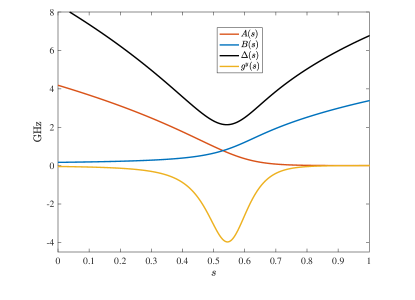
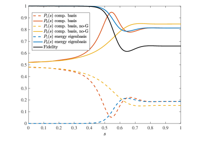
Figure 1: One qubit. (a) Annealing schedules $A(s)$ (red) and $B(s)$ (blue), gap $\Delta(s)$ (black) and the geometric term $g^{y}(s)$ (yellow) of Eq. (15). The functions $A(s)$ and $B(s)$ are obtained according to the procedure described in the SM, section C. (b) Populations of the states that are connected to the final ground state (solid) and final excited state (dashed), for $t_{f}=5$ (ns$/2\pi$). Blue and red lines represents the populations of the two states in the instantaneous energy eigenbasis [Eq. (14)] and the computational basis [Eq. (15)], respectively. Because the two Hamiltonians are equivalent up to a time-dependent basis change, and the final basis is the computational basis in both cases, the populations at the end of the evolution ($s=1$) coincide. Yellow lines represent the populations during the anneal if the geometric term of Eq. (15) is dropped. The black line is the fidelity $|\langle\psi^{\text{C}}_{1,\text{G}}(s)|\psi^{\text{C}}_{1,\text{no-G}}(s)\rangle|^{2}$ between the time-evolved states with (‘G’ subscript) and without (‘no-G’ subscript) geometric interactions. Results shown are for $\phi^{x}_{\text{CJJ}}(s)=2.9(1-s)+2.2s$ and parameter values for the flux-qubit Hamiltonian that match those of the highly coherent flux-qubits studied in Ref. Yan et al. (2016): $E_{\text{S}}/{2\pi\hbar}=3.03$GHz, $E_{\text{J}}/{2\pi\hbar}=86.2$GHz [the control fluxes $\phi^{x}_{\text{CJJ}}(s)$ and $\phi^{x}(s)$ are shown in the SM, Fig. 5].

Application to QA with superconducting flux qubits.—Let $\{|a(s)\rangle\}$ denote the $N$ lowest energy instantaneous eigenstates of the original Hamiltonian (1), i.e., $H(s)|a(s)\rangle=E_{a}(s)|a(s)\rangle$. We identify the earlier $\{|\psi^{\prime}_{a}(s)\rangle\}$ with these eigenstates, so that $W(s)$ describes the unitary evolution in the subspace rotating with the instantaneous eigenbasis of $H(s)$. In this basis, the QA process is described by the dimensionless effective Hamiltonian (6) with:

$$\tilde{H}_{ab}(s)\equiv E_{a}(s)\delta_{ab}\,,\quad G_{ab}(s)\equiv\langle a(s)|i\partial_{s}|b(s)\rangle\,.$$ (7)

In QA applications, the Hamiltonian (1) is designed such that its $N=2^{n}$ lowest energy levels can be put into $1$-to-$1$ correspondence with the energy levels of a transverse field Ising model with $n$ qubits. Thus, there exists a unitary $V(s)$ such that, up to a term proportional to the identity matrix Boixo et al. (2016a):

$$V(s)\tilde{H}(s)V^{\dagger}(s)=A(s)\tilde{H}^{X}+B(s)\tilde{H}^{Z}\,,$$ (8)

where the profile functions $A(s)$ and $B(s)$ are particular to the qubit Hamiltonian (see SM, section C), $\tilde{H}^{X}=-\sum_{i=1}^{n}\sigma_{i}^{x}$ is the usual transverse-field driver, and

$$\tilde{H}^{Z}=\sum_{i=1}^{n}h_{i}\sigma_{i}^{z}+\sum_{i>j}^{n}J_{ij}\sigma_{i}^{z}\sigma_{j}^{z}$$ (9)

is the problem Hamiltonian whose ground state encodes the answer to the optimization problem of interest. The unitary $V(s)$ is the transformation between the energy eigenbasis and the computational basis $|\psi^{\text{C}}_{a}(s)\rangle$. Note that the geometric term transforms as a geometric connection Anandan (1988) (see SM, section D):

$$G^{\text{C}}(s)=V(s)G(s)V^{\dagger}(s)+iV(s)\dot{V}^{\dagger}(s)\,.$$ (10)

Quantum annealing of a system of $n$ flux-qubits controlled by the Hamiltonian (1) is then described by the following effective Hamiltonian in the computational basis:

$$H^{\text{eff,C}}(s)=t_{f}\left(A(s)\tilde{H}^{X}+B(s)\tilde{H}^{Z}\right)-G^{\text{C}}(s)\,.$$ (11)

The first term, proportional to $t_{f}$, is the usual Hamiltonian discussed in literature in the context of QA. The second term has a geometric origin and is non-vanishing for finite annealing times $t_{f}$. The geometric term is non-stoquastic. To see this, note that the original Hamiltonian (1) is real, and thus there is a basis choice in which the energy eigenbasis states $|a(s)\rangle$ have only real amplitudes. Consequently, the geometric term $G(s)$ in Eq. (7) is then a purely imaginary Hermitian matrix. The transformed geometric term $G^{\text{C}}(s)$ [Eq. (10)] is also purely imaginary in the computational basis, since the basis change of Eq. (8) can be performed with a real unitary (i.e., orthogonal) matrix $V(s)$. Therefore, including only interactions up to two-body terms, the geometric term can be written in the most general form as follows:

$$G^{\text{C}}(s)=\sum_{i}g^{y}_{i}(s)\sigma_{i}^{y}+\sum_{i\neq j}g^{xy}_{ij}(s)\sigma_{i}^{x}\sigma_{j}^{y}+g^{zy}_{ij}(s)\sigma_{i}^{z}\sigma_{j}^{y}\,.$$ (12)

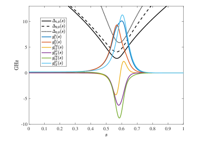
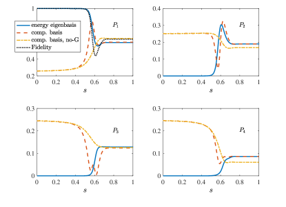
Figure 2: Two interacting qubits. (a) Gaps $\Delta_{k,0}(s)$ (black) and the geometric terms $g^{y}_{i}(s),g^{xy}_{ij}(s),g^{zy}_{ij}(s)$ computed numerically using Eq. (17) for $h_{1}=1,h_{2}=0.4,J_{12}=-0.7$. (b) Populations of the states of the instantaneous basis that are connected to the final eigenstates, for the same value of the couplings as in (a) and $t_{f}=5$ (ns$/2\pi$). The black dotted line shown in the top left panel is the fidelity as explained in Fig. 1. Results shown are for $E_{\text{C}}/{2\pi\hbar}=3.44$GHz, $E_{\text{J}}/{2\pi\hbar}=684$GHz, $E_{\text{L}}/{2\pi}=570$GHz and $E_{\text{M}}/2\pi\hbar=3.98$GHz, values that are typical for the D-Wave devices Johnson et al. (2011, 2010); Harris et al. (2010) [the control fluxes are shown in the SM, Fig. 4]. For consistency with the one C-shunt flux qubit case we set $\phi^{x}_{\text{CJJ}}(s)=2.6(1-s)+1.9s$, while in the actual DW devices the schedule is chosen such that the field $\phi^{x}(s)$ is a linear function of $s$ [we have the same characteristic parametric relationship $\phi^{x}(\phi^{x}_{\text{CJJ}})$].

Quantum annealing with geometric terms: one qubit.—We now apply the results obtained so far to QA with one qubit. For concreteness we focus on the C-shunt flux-qubit with three Josephson junctions. This qubit can be described by the following Hamiltonian Orlando et al. (1999); Yan et al. (2016); Weber et al. (2017) (see SM, section E):

$$H_{1}(\phi,s) =-\frac{1}{8}E_{\text{S}}\partial^{2}_{\phi}+P(\phi,s)$$ (13a)

$$P(\phi,s) =-2E_{\text{J}}\left(\cos[\frac{1}{2}\phi^{x}_{\text{CJJ}}(s)]\cos[\phi^{x}(s)+2\phi]+\cos\phi\right)\ ,$$ (13b)

where $\phi$ is the flux (in units of $\Phi_{0}/{2\pi}$) trapped in the superconducting ring, $E_{\text{S}}$ is the charging energy of the shunting capacitor, and $\phi^{x}_{\text{CJJ}}(s)$ and $\phi^{x}(s)$ are external fluxes used to control the anneal.

We next construct the effective Hamiltonian of Eq. (11). We start by numerically computing the ground state $|0(s)\rangle$ and first excited state $|1(s)\rangle$ of the flux-qubit Hamiltonian Eq. (13) [examples are given in the SM, Figs. 5-5], from which we numerically obtain the effective Hamiltonian [Eq. (6)] in the instantaneous energy eigenbasis:

$$H_{1}^{\text{eff}}(s)=t_{f}\frac{\Delta(s)}{2}\sigma^{z}-g(s)\sigma^{y}\,,$$ (14)

(we have ignored a term proportional to the identity matrix) where $\Delta(s)\equiv E_{1}(s)-E_{0}(s)$ is the gap [plotted in Fig. 1] and $g(s)\equiv\langle 1(s)|\partial_{s}|0(s)\rangle$. We now transform to the computational basis using the unitary $V(s)=\exp\left[\frac{i}{2}\arctan\left(\frac{A(s)}{B(s)}\right)\sigma^{y}\right]$, after which the Hamiltonian of Eq. (14) becomes

$$H_{1}^{\text{eff,C}}(s)=t_{f}\left[A(s)\sigma^{x}+B(s)\sigma^{z}\right]-g^{y}(s)\sigma^{y}\,.$$ (15)

This has the form of the most general single-qubit Hamiltonian: $H_{1}^{\text{eff,C}}(s)=\sum_{\alpha\in{x,y,z}}c_{\alpha}(s)\sigma^{\alpha}$. It can be checked easily that (see SM, section F):

$$\Delta(s) =2\sqrt{A^{2}(s)+B^{2}(s)}\,,$$ (16a)

$$g^{y}(s) =g(s)+\frac{2}{\Delta^{2}(s)}\left[\dot{A}(s)B(s)-A(s)\dot{B}(s)\right]\ .$$ (16b)

By defining the computational basis as the basis of states with well-defined persistent current, the annealing schedule functions $A(s)$ and $B(s)$ [shown in Fig. 1] can be determined in terms of the external fluxes $\phi^{x}_{\text{CJJ}}$ and $\phi^{x}$ of Eq. (13b) (see the SM, section C). Thus, Eq. (16b) shows that these flux parameters in turn control the properties of the geometric term $g^{y}$. The profile function $g^{y}(s)$ for the geometric term, also shown in Fig. 1, is non-vanishing towards the middle of the adiabatic evolution, when the gap closes. The effects of the geometric term are shown in Fig. 1, obtained by numerically solving for the corresponding unitary evolution. The effects become significant when the gap is small. There is also a significant effect on the final ground state population.

Quantum annealing with geometric terms: two qubits.—To study the interacting case, we consider two inductively-coupled compound Josephson junction flux qubits Yan et al. (2016) (see SM, section E):

$$H_{2}(\phi_{1},\phi_{2},s,h_{1},h_{2},J_{12})=H_{1}(\phi_{1},s,h_{1})+$$

$$+H_{1}(\phi_{2},s,h_{2})+P_{\text{int}}(\phi_{1},\phi_{2},s,J_{12})\,,$$ (17)

where the flux-qubit Hamiltonian is given by

$$H_{1}(\phi,s,h_{i})=-\frac{1}{4}E_{\text{C}}\partial^{2}_{\phi}+P(\phi,s,h_{i})$$ (18a)

$$P(\phi,s,h_{i})=2E_{\text{J}}\cos(\phi)\cos\left[\frac{\phi^{x}_{\text{CJJ}}(s)}{2}\right]+E_{\text{L}}\frac{\left[\phi-h_{i}\phi^{x}(s)\right]^{2}}{2}$$ (18b)

and the interaction potential is explicitly written as:

$$P_{\text{int}}(\phi_{1},\phi_{2},s,J_{12})=-J_{12}E_{\text{M}}[\phi_{1}-\phi^{x}(s)][\phi_{2}-\phi^{x}(s)]\ .$$

Proceeding as in the single qubit case, we start from the Hamiltonian (17) to numerically compute $\tilde{H}$ and $G$ appearing in Eq. (7), and construct the effective Hamiltonian in the instantaneous energy eigenbasis [Eq. (6)]. Once again, the effective Hamiltonian can be expressed in the computational basis by (numerically) finding a unitary $V$ such that the final Hamiltonian reads:

$$H_{2}^{\text{eff,C}}(s,h_{1},h_{2},J_{12})=t_{f}A(s)\left(\sigma_{1}^{x}+\sigma_{2}^{x}\right)+$$ (19)

$$+t_{f}B(s)\left(h_{1}\sigma_{1}^{z}+h_{2}\sigma_{2}^{z}+J_{12}\sigma_{1}^{z}\sigma_{2}^{z}\right)-G^{\text{C}}(s,h_{1},h_{2},J_{12})\,.$$

This is the usual transverse field Ising model, plus an additional geometric term, whose general form is given in Eq. (12). Figure 2 shows the gaps $\Delta_{k,0}=E_{k}-E_{0}$, where $\{E_{k}\}_{k=0}^{3}$ are the ordered eigenvalues of $H_{2}^{\text{eff,C}}$, and the components of the geometric term $G^{\text{C}}(s,h_{1},h_{2},J_{12})$ in the computational basis as defined in Eq. (12). Fig. 2 shows that, in general, the geometric functions $g^{y}_{i}(s),g^{xy}_{ij}(s),g^{zy}_{ij}(s)$ are all non-vanishing, and their magnitude grows as the ground state gap shrinks. In particular, as in the single-qubit case, geometric effects introduce a non-stoquastic contribution to the driver term which is non-vanishing towards the middle of the anneal. Fig. 2 shows the effect of the geometric interactions in the annealing of the system of two coupled qubits under consideration. As in the single qubit case, we see that ignoring the geometric terms results in consistently different final populations in the computational basis.

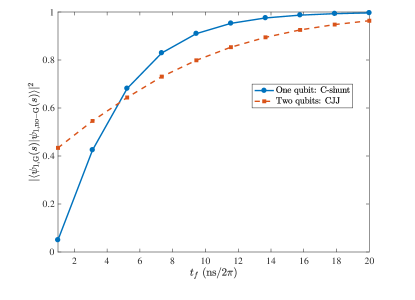
Figure 3: Fidelity at the end of the anneal as a function of the annealing time for single qubit (blue) and two qubits (red).

Dependence on the annealing time.—The contribution of the geometric terms is inherently a non-adiabatic effect, arising when diabatic transitions populate the excited states. In Fig. 3 we show the fidelity $|\langle\psi^{\text{C}}_{1,\text{G}}(s)|\psi^{\text{C}}_{1,\text{no-G}}(s)\rangle|^{2}$ between the time-evolved states with and without geometric terms, as a function of the total annealing time. As expected, the effect of the geometric terms increases with decreasing annealing time and it is reflected in the decreasing fidelity. Figure 3 shows that the total annealing time over which this contribution is significant is on the order of a few nanoseconds, for parameters relevant for current QA devices. While this is significantly shorter than the typical microsecond timescale of current QA experiments using the D-Wave devices, this is the case for the one and two-qubit cases which we have analyzed here. Since, as is clear from Eq. (16b) and from Fig. 2, the magnitude of the geometric term grows in inverse proportion to the gap, we expect it to become more significant for multi-qubit problems whose gap dependence can be inverse polynomial or even exponential. This effect is already visible in Fig. 3, which shows that the fidelity for the two-qubit system tends to be smaller than the one-qubit system for larger annealing times.

Conclusions.—We have shown that even the simplest implementation of QA with flux-qubits induces effective Hamiltonians with non-stoquastic interactions arising from a geometric phase. The appearance of such interactions is ubiquitous when the Hamiltonian of a continuous-variable system is changed over time, and the evolution is non-adiabatic, due to the appearance of the Aharanov-Anandan effect. Since arbitrarily small gaps are inevitable in QA for hard optimization problems, non-adiabatic evolutions are ultimately inescapable. We thus argue that, similarly, the geometric effects studied here are unavoidable and relevant in practical applications of QA. Moreover, since these geometric effects give rise to non-stoquastic terms in the effective Hamiltonian, they provide a natural and desirable mechanism for avoiding classically efficient simulation of QA. This may point to the possibility of “quantum supremacy” experiments with QA devices featuring fewer than $100$ physical qubits  Preskill (2012); Boixo et al. (2016b); Aaronson and Chen (2016); Fefferman et al. (2017).

Appendix A Evolution equation of the $\{|\psi^{\prime}_{a}(t)\rangle\}$ basis

Recall that the $\{|\psi_{a}(t)\rangle\}$ basis was chosen to satisfy the Schrödinger equation with the given Hamiltonian $H(t)$ [Eq. (3)]: $|\dot{\psi}_{a}(t)\rangle=-iH(t)|\psi_{a}(t)\rangle$, where in this section dot denotes $\partial_{t}$. Here we derive the evolution equation satisfied by the $\{|\psi^{\prime}_{a}(t)\rangle\}$ basis, which is related to the $\{|\psi_{a}(t)\rangle\}$ basis via the unitary $W(t)$:

$$|\psi^{\prime}_{b}(t)\rangle=\sum_{a}[W^{\dagger}(t)]_{ab}|\psi_{a}(t)\rangle\,.$$ (20)

Differentiation yields:

$$|\dot{\psi}^{\prime}_{b}(t)\rangle =\sum_{a}[\dot{W}^{\dagger}]_{ab}|\psi_{a}(t)\rangle+[W^{\dagger}(t)]_{ab}|\dot{\psi}_{a}\rangle$$

$$=\sum_{a}\left([\dot{W}^{\dagger}]_{ab}-i[W^{\dagger}(t)]_{ab}H(t)\right)|\psi_{a}(t)\rangle$$

$$=\sum_{ac}\left([\dot{W}^{\dagger}]_{ab}-i[W^{\dagger}(t)]_{ab}H(t)\right)W_{ca}(t)|\psi^{\prime}_{c}(t)\rangle$$

$$=\sum_{c}[W\dot{W}^{\dagger}]_{cb}|\psi^{\prime}_{c}(t)\rangle-iH(t)|\psi^{\prime}_{b}(t)\rangle\ .$$ (21)

Thus, the evolution equation satisfied by the basis element $|\psi^{\prime}_{a}(t)\rangle$ is

$$|\dot{\psi}^{\prime}_{a}(t)\rangle=\sum_{b}i[\tilde{H}^{\text{eff}}(t)]_{ba}|\psi^{\prime}_{b}(t)\rangle-iH(t)|\psi^{\prime}_{a}(t)\rangle\ ,$$ (22)

where we used $\dot{W}=-i{H}^{\text{eff}}(t){W}(t)$ and unitarity, and defined $\tilde{H}^{\text{eff}}(t)\equiv W^{\dagger}(t){H}^{\text{eff}}(t)W(t)$.

Appendix B Proof that $G$ is a geometric term

Let us show explicitly that $G$ is a geometric term, i.e., that $G(t)dt=G(s)ds$ where $s=\kappa^{-1}(t/t_{f})$. Note that since we assumed that $\kappa$ is invertible and differentiable, we can write $t=t_{f}\kappa(s)$, so that $dt=t_{f}\frac{d\kappa(s)}{ds}ds$ and $\partial_{t}=\frac{ds}{dt}\partial_{s}=\frac{1}{t_{f}}\left[\frac{d\kappa(s)}{ds}\right]^{-1}\partial_{s}$. Thus

$$G_{ab}(t)dt=\langle\psi^{\prime}_{a}(t)|i\partial_{t}|\psi^{\prime}_{b}(t)\rangle dt$$ (23a)

$$\quad=\langle\psi^{\prime}_{a}(s)|i\left[\frac{1}{t_{f}}\left(\frac{d\kappa(s)}{ds}\right)^{-1}\partial_{s}\right]|\psi^{\prime}_{b}(s)\rangle t_{f}\frac{d\kappa(s)}{ds}ds$$

$$\quad=G(s)ds\ ,$$ (23b)

where in the second line we used the assumption that $H(t)$ depends on $t$ only via $s$, which means, by Eq. (5a), that the same must be true of $\psi^{\prime}_{a}(t)$.

Appendix C Perturbative Derivation of Profile Functions $A(s)$ and $B(s)$

C.0.1 CJJ Flux-Qubit

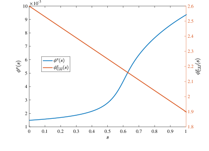
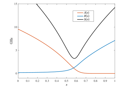
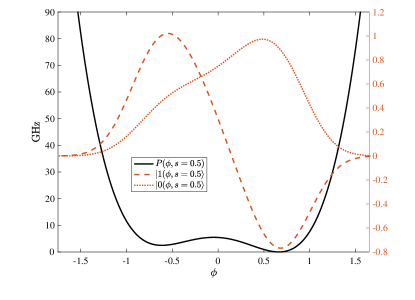
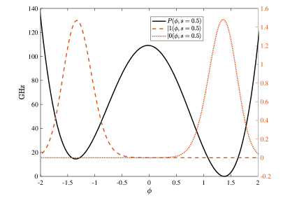
Figure 4: CJJ flux-qubit Eq. 18. (a) The $s$ dependence of the flux $\phi_{\text{CJJ}}^{x}(s)$ (right axis) controls the annealing schedule. The flux $\phi^{x}(s)$ is computed accordingly. (b) Gap and profile functions $A(s)$ and $B(s)$. (d) The potential $P(\phi,s)$ (black solid lines), and the corresponding wavefunctions of $|0(s)\rangle$ (dotted lines) and $|1(s)\rangle$ (dashed lines) for different values of the annealing parameter $s$: (c) $s=0.5$, and (d) $s=1$.

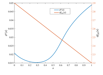
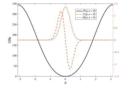
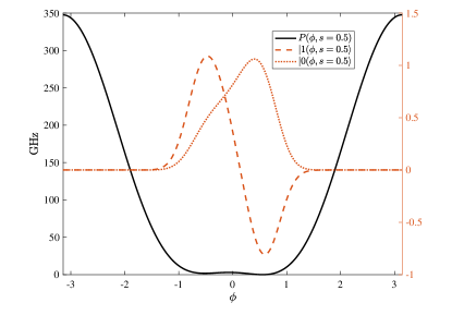
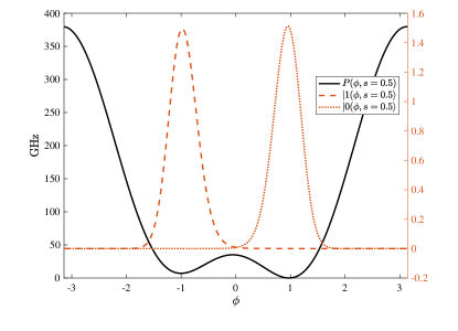
Figure 5: C-shunt flux-qubit Eq. 13. (a) The $s$ dependence of the flux $\phi_{\text{CJJ}}^{x}(s)$ (right axis) controls the annealing schedule. The flux $\phi^{x}(s)$ is computed accordingly. (b)-(d) The potential $P(\phi,s)$ (black solid lines), and the corresponding wave functions of $|0(s)\rangle$ (dotted lines) and $|1(s)\rangle$ (dashed lines) for different values of the annealing parameter $s$: (b) $s=0$, (c) $s=0.5$, and (d) $s=1$.

In this section we closely follow Ref. Boixo et al. (2016a) to briefly describe how the annealing profile functions $A(s)$ and $B(s)$ can be calculated. The main observation is that the control flux $\phi^{x}$, i.e., the bias between the two potential wells, is a small perturbation for the potential of $H_{1}$ in Eq. (18). The eigenstates $|0(s)\rangle$ and $|1(s)\rangle$ of the unperturbed Hamiltonian with $\phi^{x}=0$ are used to define the states of the computational basis:

$$|\!\uparrow~{}\!\!\!(s)\rangle \equiv \frac{1}{\sqrt{2}}\left(|1(s)\rangle+|0(s)\rangle\right){|_{\phi^{x}=0}}$$

$$|\!\downarrow~{}\!\!\!(s)\rangle \equiv \frac{1}{\sqrt{2}}\left(|1(s)\rangle-|0(s)\rangle\right){|_{\phi^{x}=0}}\,.$$ (24)

These symmetric and antisymmetric combinations have opposite and well-defined circulating persistent current along the whole anneal, with the persistent current operator defined as $I_{\text{p}}=E_{\text{L}}\phi$. This justifies the use of $|\!\uparrow~{}\!\!\!(s)\rangle$ and $|\!\downarrow~{}\!\!\!(s)\rangle$ as states of the computational basis.

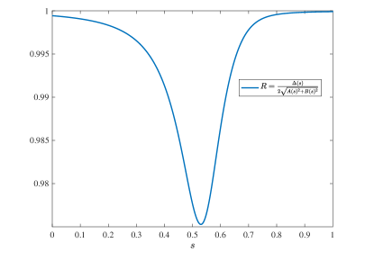
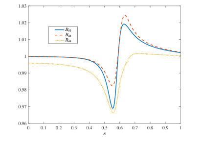
Figure 6: (a) One C-shunt flux-qubit with: ratio between the exact gap $\Delta(s)$ and the gap estimated via the perturbative approach described in section C used to define the computational basis along the anneal and compute the profile functions $A(s)$ and $B(s)$. (b) Two coupled CJJ flux-qubits with $h_{1}=1,h_{2}=0.4,J_{12}=-0.7$: similar ratios between the exact gaps and the gaps computed with the Hamiltonian written in the computational basis. Note that the exact gaps are well approximated by the mapping to the computational basis described in section C. The difference is largest towards the middle of the anneal, where the first order approximation in the control flux $\phi^{x}$ is is less accurate.

We can now expand the flux qubit Hamiltonian $H_{1}$ in Eq. (18) to first order in $\phi^{x}$ to get:

$$H_{1}(s,\phi^{x})=H_{1}(s,\phi^{x}=0)+\phi^{x}(s)I_{\text{p}}+\mathcal{O}[(\phi^{x})^{2}]\,.$$ (25)

Evaluating the Hamiltonian above in the basis $(|\!\uparrow~{}\!\!\!(s)\rangle,|\!\downarrow~{}\!\!\!(s)\rangle)$ then gives (up to a term proportional to identity) the Hamiltonian:

$$H_{1}=A(s)\sigma^{x}+B(s)\sigma^{z}\,,$$ (26)

where

$$A(s) \equiv\langle\uparrow~{}\!\!\!(s)|H_{1}(s,\phi^{x}=0)|\!\downarrow~{}\!\!\!(s)\rangle$$

$$B(s) \equiv\langle\uparrow~{}\!\!\!(s)|\phi^{x}(s)I_{\text{p}}|\!\uparrow~{}\!\!\!(s)\rangle\equiv\phi^{x}(s)I_{\text{p}}(s)\,.$$ (27)

The profile functions above are completely controlled via the external fluxes $\phi_{\text{CJJ}}(s)$ and $\phi^{x}(s)$.

The schedule of the flux $\phi^{x}(s)$ and thus of the profile function $B(s)$ is further constrained in the case of multi-qubit interactions. The interaction potential is given by Eq. (Non-Stoquastic Interactions in Quantum Annealing via the Aharonov-Anandan Phase), whose expectation value in the computational basis is given by:

$$\langle\uparrow_{1}~{}\!\!\!(s)~{}\!\!\!\uparrow_{2}~{}\!\!\!(s)|P_{\text{int}}|~{}\!\!\!\uparrow_{1}~{}\!\!\!(s)~{}\!\!\!\uparrow_{2}~{}\!\!\!(s)\rangle\simeq-J_{12}E_{\text{M}}E_{\text{L}}^{-2}I_{\text{p}}(s)^{2}\,,$$ (28)

from which it follows that the interaction term in the effective Hamiltonian is given by $H_{\text{int}}=-J_{12}E_{\text{M}}E_{\text{L}}^{-2}I_{\text{p}}(s)^{2}\sigma_{1}^{z}\sigma_{2}^{z}$. To ensure the same annealing schedule for the local and interaction terms, the control field $\phi^{x}$ is then chosen to be proportional to the persistent current $\phi^{x}(s)=E_{\text{M}}E_{\text{L}}^{-2}I_{\text{p}}(s)$. This implies that $B(s)=E_{\text{M}}E_{\text{L}}^{-2}I_{\text{p}}(s)^{2}$.

We have considered an annealing schedule linear in the control field $\phi_{\text{CJJ}}(s)$ [see Fig. 4]. The corresponding values for the control flux $\phi^{x}(s)$ and profile functions $A(s)$ and $B(s)$ are shown in Fig. 4 and are computed using the prescription described in this section, using the numerical methods of the next section. Figure 6 shows the ratios between the exact gaps computed by numerical diagonalization of Eqs. (13) and (17), and the gaps computed by diagonalizing the Hamiltonians Eqs. (15) and (19) (without geometric terms), when the profile functions $A(s)$ and $B(s)$ are computed as described in this section. Due to the perturbative expansion, the method described in this section only approximately recovers the exact gaps. The relative error is largest (up to 2%) in the middle of the anneal, when the gaps close.

C.0.2 C-shunt Flux-Qubit

As in the CJJ case, we will treat $\phi^{x}$ as a small perturbation. Expanding the Hamiltonian (13) to first order in $\phi^{x}$ gives:

$$H_{1}(\phi^{x})=H_{1}(\phi^{x}=0)+2E_{\text{J}}\phi^{x}\cos(\phi^{x}_{\text{CJJ}}/2)\sin(2\phi)\,.$$ (29)

The Hamiltonian above has the following representation:

$$H_{1}=A(s)\sigma^{x}+B(s)\sigma^{z}\,,$$ (30)

with

$$A(s) =\left(\langle\uparrow~{}\!\!\!(s)|H(s,\phi^{x}=0)|\!\downarrow~{}\!\!\!(s)\rangle\right.$$

$$B(s) =2E_{\text{J}}\phi^{x}\cos[\phi^{x}_{\text{CJJ}}(s)/2]\langle\uparrow~{}\!\!\!(s)|\sin(2\phi_{m})|\!\uparrow~{}\!\!\!(s)\rangle\equiv$$

$$\equiv\phi^{x}\mathcal{I}_{\text{p}}(s)\,.$$ (31)

For consistency with the CJJ example, we have taken $\phi^{x}(s)\equiv E_{\text{M}}E_{\text{L}}^{-2}I_{\text{p}}(s)^{2}/\mathcal{I}_{\text{p}}(s)\$ with $E_{\text{M}}^{-1}E_{\text{L}}^{2}=10^{4}$GHz, such that $B(s)$ is proportional to the square of the persistent current.

Appendix D Proof that $G$ transforms as a geometric connection

(a)  

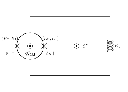
(b)  

Figure 7: (a) Compound Josephson Junction flux-qubit. (b) Capacitively shunted flux-qubit.

Let us show that $G$ transforms as in Eq. (10), i.e., that $G^{\text{C}}(s)=V(s)G(s)V^{\dagger}(s)+iV(s)\dot{V}^{\dagger}(s)$.

Recall that we transform from the basis $|a(s)\rangle$ (e.g., the energy eigenbasis) to the new basis $|\psi^{\text{C}}_{a}(s)\rangle$ (e.g., the computational basis) using the unitary $V(s)$. Thus, $|a(s)\rangle=\sum_{b}V_{ba}(s)|\psi^{\text{C}}_{b}(s)\rangle$. From now on we drop the explicit $s$-dependence for simplicity. By definition, $G^{\text{C}}_{ab}=\langle\psi^{\text{C}}_{a}|G^{\text{C}}|\psi^{\text{C}}_{b}\rangle=i\langle\psi^{\text{C}}_{a}|\dot{\psi}^{\text{C}}_{b}\rangle$. Using these two expressions, we have:

$$G_{ab} =\langle a|G|b\rangle=i\langle a|\dot{b}\rangle=$$ (32a)

$$=i\sum_{cd}\langle\psi^{\text{C}}_{c}(s)|V^{\dagger}_{ac}\left[\dot{V}_{bd}|\psi^{\text{C}}_{b}(s)\rangle+{V}_{bd}|\dot{\psi}^{\text{C}}_{b}(s)\rangle\right]$$ (32b)

$$=i\sum_{d}V^{\dagger}_{ab}\dot{V}_{bd}+\sum_{cd}V^{\dagger}_{ac}G^{\text{C}}_{cb}{V}_{bd}$$ (32c)

$$=i(V^{\dagger}\dot{V})_{ab}+(V^{\dagger}G^{\text{C}}V)_{ab}\ ,$$ (32d)

i.e., $G^{\text{C}}=VGV^{\dagger}-i\dot{V}V^{\dagger}$, which gives the desired result after using unitarity to write $\dot{V}{V}^{\dagger}=-V\dot{V}^{\dagger}$.

Appendix E Flux-Qubit Hamiltonians

The Langrangian of a superconducting circuit with Josephson junctions is generically written as follows Makhlin et al. (2001):

$$\mathcal{L}=\frac{1}{2}\sum_{c}E_{\text{C},c}^{-1}\dot{\phi}^{2}_{c}+\sum_{j}E_{\text{J},j}\cos\phi_{j}-\sum_{l}\frac{1}{2}E_{\text{L},l}{(\phi_{l}-\phi_{l}^{x})^{2}}\,,$$ (33)

where the first term is the kinetic term, the second is the junction energy, and the third is the induction energy. The $\phi_{c}$ are the phase differences at each capacitance. The charging energy is $E_{\text{C},c}\equiv{(2e)^{2}}/{C_{c}}$, where $C_{c}$ is the $c$-th capacitance and $e$ the electron charge. The junction energies are given by $E_{\text{J},j}\equiv I_{c,j}(\Phi_{0}/{2\pi})$, where $I_{c,j}$ is the critical current of the $j$-th junction. The induction energies are given by $E_{\text{L},l}\equiv(\Phi_{0}/{2\pi})^{2}/L_{l}$, where $L_{l}$ is the induction of the $l$-th loop. The conjugate momenta are $p_{c}=\partial\mathcal{L}/\partial{\dot{\phi}_{c}}=E_{C,c}^{-1}\dot{\phi}_{c}$. The circuit is quantized by promoting the momenta to operators: $p_{c}\mapsto-i\partial_{\phi_{c}}$. The corresponding Hamiltonian is:

$$H=-\sum_{c}\frac{E_{\text{C},c}}{2}\partial_{\phi_{c}}^{2}-\sum_{j}E_{\text{J},j}\cos\phi_{j}+\sum_{l}\frac{E_{\text{L},l}}{2}{(\phi_{l}-\phi_{l}^{x})^{2}}\,.$$

E.0.1 Compound Josephson Junction (CJJ) Flux-Qubit

The basic design of a CJJ flux-qubit Yan et al. (2016) is shown in Fig. 7(a). We assume the same charging and junction energies for the two Josephson junctions and a negligible inductance of the small loop. The Hamiltonian for this device can then be written as:

$$H_{\text{CJJ}} = -\frac{1}{2}E_{\text{C}}\left(\partial^{2}_{\phi_{L}}+\partial^{2}_{\phi_{R}}\right)-E_{\text{J}}\left(\cos\phi_{L}+\cos\phi_{R}\right)+$$ (34)

$$+ \frac{1}{2}E_{\text{L}}[(\phi_{L}-\phi_{R})/2-\phi^{x}]^{2}\,,$$

i.e., the sum of the charging, junction and induction energies of the circuit. By defining $\phi\equiv(\phi_{L}-\phi_{R})/2$ and $\phi_{\text{CJJ}}=\phi_{R}+\phi_{L}$ we have $\partial_{\phi_{L,R}}=\partial_{\phi_{\text{CJJ}}}\pm 1/2\partial_{\phi}$ , from which we obtain:

$$H_{\text{CJJ}} = -\frac{1}{2}\frac{E_{\text{C}}}{2}\partial^{2}_{\phi}-2E_{\text{J}}\cos\left(\frac{\phi^{x}_{\text{CJJ}}}{2}\right)\cos\phi+E_{\text{L}}\frac{(\phi-\phi^{x})^{2}}{2}\,.$$

where we have neglected the term $-\frac{1}{2}(2E_{\text{C}})\partial^{2}_{\phi_{\text{CJJ}}}$ since the small loop inductance gives $\phi^{x}_{\text{CJJ}}=\phi_{\text{CJJ}}$, i.e., the flux $\phi_{\text{CJJ}}$ is locked to the external flux $\phi^{x}_{\text{CJJ}}$. The equation above reduces to Eq. (18) with the redefinition $\phi^{x}_{\text{CJJ}}\mapsto 2\pi-\phi^{x}_{\text{CJJ}}$.

E.0.2 Capacitively Shunted (C-shunt) Flux-Qubit

The basic design of a C-shunt flux-qubit Orlando et al. (1999); Yan et al. (2016) involves four Josephson junctions and a large shunting capacitance and is shown in Fig. 7(b). We start by writing the kinetic term:

$$K=\frac{1}{2}E_{\text{C}}^{-1}\left(\dot{\phi}^{2}_{1}+\dot{\phi}^{2}_{2}+\dot{\phi}_{L}^{2}+\dot{\phi}_{R}^{2}\right)+\frac{1}{2}E^{-1}_{\text{S}}\left(\dot{\phi}_{1}-\dot{\phi}_{2}\right)^{2}\,,\\$$ (36)

where the first term comes from the junctions while the last term is the shunting capacitor energy with $E_{\text{S}}={(2e)^{2}}/{C_{\text{S}}}$. By defining $\phi_{\text{CJJ}}=\phi_{R}+\phi_{L}$, $\phi=(\phi_{L}-\phi_{R})/2+\phi_{2}-\phi_{1}$ and $\phi_{\pm}=(\phi_{1}\pm\phi_{2})/2$ we get $\dot{\phi}_{1,2}=\dot{\phi}_{+}\pm\dot{\phi}_{-}$ and $\dot{\phi}_{R}=-\dot{\phi}_{L}=-2\dot{\phi}_{-}$, where we have set $\dot{\phi}_{\text{CJJ}}=\dot{\phi}=0$, i.e., the fluxes $\phi_{\text{CJJ}}$ and $\phi$ are constant and locked to the external fluxes ($\phi_{\text{CJJ}}=\phi^{x}_{\text{CJJ}}$, $\phi=\phi^{x}$) due to the small inductances. We can then rewrite $K$ in Eq. (36) as

$$K = \frac{1}{2}E_{\text{C}}^{-1}\left(2\dot{\phi}^{2}_{+}+10\dot{\phi}^{2}_{-}\right)+\frac{1}{2}\left(\frac{E_{\text{S}}}{4}\right)^{-1}\dot{\phi}^{2}_{-}\simeq$$ (37)

$$\simeq \frac{1}{2}\left(\frac{E_{\text{S}}}{4}\right)^{-1}\dot{\phi}^{2}_{-}\,,$$

where in the last step we neglected the light (high-frequency) mode $\phi_{+}$ ($E_{\text{S}}\ll E_{\text{C}}$ due to the large shunting capacitance). The potential term due to the Josephson junctions is just the sum of the four junction energies:

$$P = -E_{\text{J}}\left(\cos\phi_{1}+\cos\phi_{2}+\cos\phi_{L}+\cos\phi_{R}\right)$$

$$= -2E_{\text{J}}\left[\cos\phi_{-}\cos\phi_{+}+\cos(\phi^{x}_{\text{CJJ}}/2)\cos(\phi^{x}+2\phi_{-})\right]\,.$$

We then get the final Hamiltonian for the C-shunt qubit:

$$H = -\frac{1}{2}\left(\frac{E_{\text{S}}}{4}\right)\partial^{2}_{\phi_{-}}+$$

$$- 2E_{\text{J}}\left[\cos\phi_{-}\cos\phi_{+}+\cos(\phi^{x}_{\text{CJJ}}/2)\cos(\phi^{x}+2\phi_{-})\right]\,,$$

which reduces to Eq. (13) after we set $\phi_{+}=0$ (i.e. the value that minimize the potential), and rename $\phi_{-}\mapsto\phi$.

Appendix F Derivation of Eq. (16)

The effective Hamiltonian Eq. (14) $H_{1}^{\text{eff}}(s)=t_{f}\frac{\Delta(s)}{2}\sigma^{z}-g(s)\sigma^{y}$ is written in the basis defined by the instantaneous energy eigenbasis. A more conventional choice is to rewrite the Hamiltonian above in the computational basis, as in Eq. (15). This can be done via a unitary transformation of the form

$$V(s)=\exp\left[i\theta(s)\,\sigma^{y}\right]\,,$$ (40)

with $\theta(s)$ to be determined. Now,

$$V(s)\sigma^{z}V^{\dagger}(s)=-\sin[2\theta(s)]\sigma^{x}+\cos[2\theta(s)]\sigma^{z}\,,$$ (41)

from which we find, using Eq. (8):

$$A(s)=\frac{\Delta(s)}{2}\sin[2\theta(s)]\,,\quad B(s)=\frac{\Delta(s)}{2}\cos[2\theta(s)]\ ,$$ (42)

from which Eq. (16a) follows. For the geometric term we use Eq. (10) to get

$$g^{y}(s)\sigma^{y} \equiv V(s)g(s)\sigma^{y}V^{\dagger}(s)+iV(s)\dot{V}^{\dagger}(s)$$

$$=\left[g(s)+\dot{\theta}(s)\right]\sigma^{y}\,.$$ (43)

Since $\theta(s)=\arctan[A(s)/B(s)]/2$, we have:

$$\dot{\theta}(s)=\frac{2}{\Delta^{2}(s)}\left[\dot{A}(s)B(s)-A(s)\dot{B}(s)\right]\,.$$ (44)

Combining the last two equations yields Eq. (16b) reported in the main text.

Appendix G Numerical Methodology

All the “static” quantities, e.g., the quantities shown in Figs. 1, 2, 4, 5 and 6, are determined at a given value of the schedule parameter $s$ by first numerically computing the wave functions $|0(s)\rangle$ and $|1(s)\rangle$ [see, e.g., Fig. 4 and Fig. 5]. We first discretized the flux-qubit Hamiltonian Eq. (1). For example, the one-qubit Hamiltonian Eq. (13a) is reduced to the following $L$-dimensional system:

$$H_{1}^{\text{discr}}({\phi},s,h)\approx-\frac{E_{\text{C}}}{8}\frac{(L-1)^{2}}{(\phi_{L}-\phi_{-L})^{2}}\left(\begin{array}[]{cccc}-2&1&&\\ 1&\ddots&\ddots&\\ &\ddots&\ddots&1\\ &&1&-2\end{array}\right)+$$ (49)

$$+\left(\begin{array}[]{cccc}P(\phi_{0},s,h)&&&\\ &P(\phi_{1},s,h)&&\\ &&\ddots&\\ &&&P(\phi_{L-1},s,h)\end{array}\right)\,,$$ (54)

where the first term is the discretized Laplacian and the continuous flux $\phi$ is discretized as $\phi_{i}=\phi_{-L}+i(\phi_{L}-\phi_{-L})/(L-1)$, $i=0,\dots,L-1$, with $L$ being the size of the mesh. Similarly we can discretize the two-qubit Hamiltonian Eq. (17) to obtain an $L^{2}$-dimensional system. We used $L=600$, which was sufficient for numerical convergence. We numerically computed all the static functions on a mesh of $100$ points for the annealing parameter $s$. The value of all functions at all other intermediate points, when required, where computed via a cubic interpolation.

Once all the static quantities where computed, the “dynamic” quantities of Figs. 1, 2 and 3 were computed by solving the Schrödinger equations resulting from the effective one- and two-qubit Hamiltonians Eqs. (14), (15) and (19). We used a standard ode45 solver provided with Matlab.

References

- Farhi et al. (2000) Edward Farhi, Jeffrey Goldstone, Sam Gutmann, and Michael Sipser, “Quantum Computation by Adiabatic Evolution,” arXiv:quant-ph/0001106 (2000).
- Farhi et al. (2001) Edward Farhi, Jeffrey Goldstone, Sam Gutmann, Joshua Lapan, Andrew Lundgren, and Daniel Preda, “A Quantum Adiabatic Evolution Algorithm Applied to Random Instances of an NP-Complete Problem,” Science 292, 472–475 (2001).
- van Dam et al. (8-11 Oct. 2001) W. van Dam, M. Mosca, and U. Vazirani, “How powerful is adiabatic quantum computation?” Foundations of Computer Science, 2001. Proceedings. 42nd IEEE Symposium on, Foundations of Computer Science, 2001. Proceedings. 42nd IEEE Symposium on , 279–287 (8-11 Oct. 2001).
- Aharonov et al. (2007) Dorit Aharonov, Wim van Dam, Julia Kempe, Zeph Landau, Seth Lloyd, and Oded Regev, “Adiabatic quantum computation is equivalent to standard quantum computation,” SIAM J. Comput. 37, 166–194 (2007).
- Albash and Lidar (2016) Tameem Albash and Daniel A. Lidar, “Adiabatic quantum computing,” arXiv:1611.04471 (2016).
- Kadowaki and Nishimori (1998) Tadashi Kadowaki and Hidetoshi Nishimori, “Quantum annealing in the transverse Ising model,” Phys. Rev. E 58, 5355 (1998).
- Santoro et al. (2002) Giuseppe E. Santoro, Roman Martoňák, Erio Tosatti, and Roberto Car, “Theory of quantum annealing of an Ising spin glass,” Science 295, 2427–2430 (2002).
- Das and Chakrabarti (2008) Arnab Das and Bikas K. Chakrabarti, “Colloquium: Quantum annealing and analog quantum computation,” Rev. Mod. Phys. 80, 1061–1081 (2008).
- Brooke et al. (2001) J. Brooke, T. F. Rosenbaum, and G. Aeppli, “Tunable quantum tunnelling of magnetic domain walls,” Nature 413, 610–613 (2001).
- Johnson et al. (2011) M. W. Johnson, M. H. S. Amin, S. Gildert, T. Lanting, F. Hamze, N. Dickson, R. Harris, A. J. Berkley, J. Johansson, P. Bunyk, E. M. Chapple, C. Enderud, J. P. Hilton, K. Karimi, E. Ladizinsky, N. Ladizinsky, T. Oh, I. Perminov, C. Rich, M. C. Thom, E. Tolkacheva, C. J. S. Truncik, S. Uchaikin, J. Wang, B. Wilson, and G. Rose, “Quantum annealing with manufactured spins,” Nature 473, 194–198 (2011).
- Johnson et al. (2010) M W Johnson, P Bunyk, F Maibaum, E Tolkacheva, A J Berkley, E M Chapple, R Harris, J Johansson, T Lanting, I Perminov, E Ladizinsky, T Oh, and G Rose, “A scalable control system for a superconducting adiabatic quantum optimization processor,” Superconductor Science and Technology 23, 065004 (2010).
- Harris et al. (2010) R. Harris, M. W. Johnson, T. Lanting, A. J. Berkley, J. Johansson, P. Bunyk, E. Tolkacheva, E. Ladizinsky, N. Ladizinsky, T. Oh, F. Cioata, I. Perminov, P. Spear, C. Enderud, C. Rich, S. Uchaikin, M. C. Thom, E. M. Chapple, J. Wang, B. Wilson, M. H. S. Amin, N. Dickson, K. Karimi, B. Macready, C. J. S. Truncik, and G. Rose, “Experimental investigation of an eight-qubit unit cell in a superconducting optimization processor,” Phys. Rev. B 82, 024511 (2010).
- McMahon et al. (2016) Peter L. McMahon, Alireza Marandi, Yoshitaka Haribara, Ryan Hamerly, Carsten Langrock, Shuhei Tamate, Takahiro Inagaki, Hiroki Takesue, Shoko Utsunomiya, Kazuyuki Aihara, Robert L. Byer, M. M. Fejer, Hideo Mabuchi, and Yoshihisa Yamamoto, “A fully-programmable 100-spin coherent Ising machine with all-to-all connections,” Science (2016).
- Bravyi et al. (2008) Sergey Bravyi, David P. DiVincenzo, Roberto I. Oliveira, and Barbara M. Terhal, “The complexity of stoquastic local hamiltonian problems,” Quant. Inf. Comp. 8, 0361 (2008).
- Bravyi and Terhal (2009) S. Bravyi and B. Terhal, “Complexity of stoquastic frustration-free hamiltonians,” SIAM Journal on Computing, SIAM Journal on Computing 39, 1462–1485 (2009).
- Farhi and Harrow (2016) Edward Farhi and Aram W. Harrow, “Quantum supremacy through the quantum approximate optimization algorithm,” arXiv:1602.07674 (2016).
- Heim et al. (2015) Bettina Heim, Troels F. Rønnow, Sergei V. Isakov, and Matthias Troyer, “Quantum versus classical annealing of Ising spin glasses,” Science 348, 215–217 (2015).
- Bravyi and Gosset (2016) Sergey Bravyi and David Gosset, “Polynomial-time classical simulation of quantum ferromagnets,” arXiv:1612.05602 (2016).
- Hastings and Freedman (2013) M. B. Hastings and M. H. Freedman, “Obstructions to classically simulating the quantum adiabatic algorithm,” arXiv:1302.5733 (2013).
- Jarret et al. (2016) Michael Jarret, Stephen P. Jordan, and Brad Lackey, “Adiabatic optimization versus diffusion monte carlo methods,” Physical Review A 94, 042318– (2016).
- Farhi et al. (2011) Edward Farhi, Jeffrey Goldstone, David Gosset, Sam Gutmann, Harvey B. Meyer, and Peter Shor, “Quantum adiabatic algorithms, small gaps, and different paths,” Quantum Info. Comput. 11, 181–214 (2011).
- Seoane and Nishimori (2012) Beatriz Seoane and Hidetoshi Nishimori, “Many-body transverse interactions in the quantum annealing of the p -spin ferromagnet,” J. Phys. A 45, 435301 (2012).
- Crosson et al. (2014) Elizabeth Crosson, Edward Farhi, Cedric Yen-Yu Lin, Han-Hsuan Lin, and Peter Shor, “Different strategies for optimization using the quantum adiabatic algorithm,” arXiv preprint arXiv:1401.7320 (2014).
- Seki and Nishimori (2015) Yuya Seki and Hidetoshi Nishimori, “Quantum annealing with antiferromagnetic transverse interactions for the Hopfield model,” J. Phys. A 48, 335301 (2015).
- Zeng et al. (2016) Lishan Zeng, Jun Zhang, and Mohan Sarovar, “Schedule path optimization for adiabatic quantum computing and optimization,” Journal of Physics A: Mathematical and Theoretical 49, 165305 (2016).
- Hormozi et al. (2016) L. Hormozi, E. W. Brown, G. Carleo, and M. Troyer, “Non-Stoquastic Hamiltonians and Quantum Annealing of Ising Spin Glass,” arXiv:1609.06558 (2016).
- Nishimori and Takada (2016) Hidetoshi Nishimori and Kabuki Takada, “Exponential Enhancement of the Efficiency of Quantum Annealing by Non-Stochastic Hamiltonians,” arXiv:1609.03785 (2016).
- Shin et al. (2014) Seung Woo Shin, Graeme Smith, John A. Smolin, and Umesh Vazirani, “How “quantum” is the D-Wave machine?” arXiv:1401.7087 (2014).
- Albash et al. (2015a) Tameem Albash, Walter Vinci, Anurag Mishra, Paul A. Warburton, and Daniel A. Lidar, “Consistency tests of classical and quantum models for a quantum annealer,” Phys. Rev. A 91, 042314– (2015a).
- Albash et al. (2015b) T. Albash, T. F. Rønnow, M. Troyer, and D. A. Lidar, “Reexamining classical and quantum models for the D-Wave One processor,” Eur. Phys. J. Spec. Top. 224, 111–129 (2015b).
- Lanting et al. (2014) T. Lanting, A. J. Przybysz, A. Yu. Smirnov, F. M. Spedalieri, M. H. Amin, A. J. Berkley, R. Harris, F. Altomare, S. Boixo, P. Bunyk, N. Dickson, C. Enderud, J. P. Hilton, E. Hoskinson, M. W. Johnson, E. Ladizinsky, N. Ladizinsky, R. Neufeld, T. Oh, I. Perminov, C. Rich, M. C. Thom, E. Tolkacheva, S. Uchaikin, A. B. Wilson, and G. Rose, “Entanglement in a quantum annealing processor,” Phys. Rev. X 4, 021041– (2014).
- Boixo et al. (2016a) Sergio Boixo, Vadim N. Smelyanskiy, Alireza Shabani, Sergei V. Isakov, Mark Dykman, Vasil S. Denchev, Mohammad H. Amin, Anatoly Yu Smirnov, Masoud Mohseni, and Hartmut Neven, “Computational multiqubit tunnelling in programmable quantum annealers,” Nat Commun 7 (2016a).
- Albash et al. (2015c) Tameem Albash, Itay Hen, Federico M. Spedalieri, and Daniel A. Lidar, “Reexamination of the evidence for entanglement in a quantum annealer,” Physical Review A 92, 062328– (2015c).
- Boixo et al. (2014) Sergio Boixo, Troels F. Ronnow, Sergei V. Isakov, Zhihui Wang, David Wecker, Daniel A. Lidar, John M. Martinis, and Matthias Troyer, “Evidence for quantum annealing with more than one hundred qubits,” Nat. Phys. 10, 218–224 (2014).
- Rønnow et al. (2014) Troels F. Rønnow, Zhihui Wang, Joshua Job, Sergio Boixo, Sergei V. Isakov, David Wecker, John M. Martinis, Daniel A. Lidar, and Matthias Troyer, “Defining and detecting quantum speedup,” Science 345, 420–424 (2014).
- Hen et al. (2015) Itay Hen, Joshua Job, Tameem Albash, Troels F. Rønnow, Matthias Troyer, and Daniel A. Lidar, “Probing for quantum speedup in spin-glass problems with planted solutions,” Phys. Rev. A 92, 042325– (2015).
- Martin-Mayor and Hen (2015) Victor Martin-Mayor and Itay Hen, “Unraveling quantum annealers using classical hardness,” Scientific Reports 5, 15324 EP – (2015).
- King et al. (2015) Andrew D. King, Trevor Lanting, and Richard Harris, “Performance of a quantum annealer on range-limited constraint satisfaction problems,” arXiv:1502.02098 (2015).
- Mandrà et al. (2016) Salvatore Mandrà, Zheng Zhu, Wenlong Wang, Alejandro Perdomo-Ortiz, and Helmut G. Katzgraber, “Strengths and weaknesses of weak-strong cluster problems: A detailed overview of state-of-the-art classical heuristics versus quantum approaches,” Physical Review A 94, 022337– (2016).
- Vinci and Lidar (2016) Walter Vinci and Daniel A. Lidar, “Optimally stopped optimization,” Physical Review Applied 6, 054016– (2016).
- Aharonov and Anandan (1987) Yakir Aharonov and J Anandan, “Phase change during a cyclic quantum evolution,” Physical Review Letters 58, 1593 (1987).
- Anandan (1988) J. Anandan, “Non-adiabatic non-abelian geometric phase,” Physics Letters A 133, 171 – 175 (1988).
- Makhlin et al. (2001) Yuriy Makhlin, Gerd Schön, and Alexander Shnirman, “Quantum-state engineering with Josephson-junction devices,” Rev. Mod. Phys. 73, 357–400 (2001).
- Berry (1984) M. V. Berry, “Quantal phase factors accompanying adiabatic changes,” Proceedings of the Royal Society of London. A. Mathematical and Physical Sciences 392, 45 (1984).
- Wilczek and Zee (1984) Frank Wilczek and A. Zee, “Appearance of gauge structure in simple dynamical systems,” Phys. Rev. Lett. 52, 2111–2114 (1984).
- Yan et al. (2016) Fei Yan, Simon Gustavsson, Archana Kamal, Jeffrey Birenbaum, Adam P Sears, David Hover, Ted J. Gudmundsen, Danna Rosenberg, Gabriel Samach, S Weber, Jonilyn L. Yoder, Terry P. Orlando, John Clarke, Andrew J. Kerman, and William D. Oliver, “The flux qubit revisited to enhance coherence and reproducibility,” Nature Communications 7, 12964 EP – (2016).
- Orlando et al. (1999) T. P. Orlando, J. E. Mooij, Lin Tian, Caspar H. van der Wal, L. S. Levitov, Seth Lloyd, and J. J. Mazo, “Superconducting persistent-current qubit,” Phys. Rev. B 60, 15398–15413 (1999).
- Weber et al. (2017) Steven J. Weber, Gabriel O. Samach, David Hover, Simon Gustavsson, David K. Kim, Danna Rosenberg, Adam P. Sears, Fei Yan, Jonilyn L. Yoder, William D. Oliver, and Andrew J. Kerman, “Coherent coupled qubits for quantum annealing,” arXiv:1701.06544 (2017).
- Preskill (2012) J. Preskill, “The Theory of the Quantum World (Proceedings of the 25th Solvay Conference on Physics),” (World Scientific, Singapore, 2012) p. 63.
- Boixo et al. (2016b) Sergio Boixo, Sergei V. Isakov, Vadim N. Smelyanskiy, Ryan Babbush, Nan Ding, Zhang Jiang, John M. Martinis, and Hartmut Neven, “Characterizing quantum supremacy in near-term devices,” arXiv:1608.00263 (2016b).
- Aaronson and Chen (2016) Scott Aaronson and Lijie Chen, “Complexity-theoretic foundations of quantum supremacy experiments,” arXiv:1612.05903 (2016).
- Fefferman et al. (2017) Bill Fefferman, Michael Foss-Feig, and Alexey V. Gorshkov, “Exact sampling hardness of Ising spin models,” arXiv:1701.03167 (2017).