Joint Power Allocation and Beamforming for Energy-Efficient Two-Way Multi-Relay Communications

Abstract

This paper considers the joint design of user power allocation and relay beamforming in relaying communications, in which multiple pairs of single-antenna users exchange information with each other via multiple-antenna relays in two time slots. All users transmit their signals to the relays in the first time slot while the relays broadcast the beamformed signals to all users in the second time slot. The aim is to maximize the system’s energy efficiency (EE) subject to quality-of-service (QoS) constraints in terms of exchange throughput requirements. The QoS constraints are nonconvex with many nonlinear cross-terms, so finding a feasible point is already computationally challenging. The sum throughput appears in the numerator while the total consumption power appears in the denominator of the EE objective function. The former is a nonconcave function and the latter is a nonconvex function, making fractional programming useless for EE optimization. Nevertheless, efficient iterations of low complexity to obtain its optimized solutions are developed. The performances of the multiple-user and multiple-relay networks under various scenarios are evaluated to show the merit of the paper development.

I Introduction

Two-way relaying (TWR) [1, 2, 3] has been the focus of considerable research interest in recent years due to its potential in offering higher information exchange throughput for cognitive communications such as device-to-device (D2D) and machine-to-machine (M2M) communications [4, 5]. Unlike the conventional one-way relaying, which needs four time slots for information exchange between a pair of users (UEs), TWR needs just two time slots for this exchange [6, 7, 2]. In the first time slot, known as the multiple access (MAC) phase, all UEs simultaneously transmit their signals to the relays. In the second time slot, also known as the broadcast (BC) phase, the relays broadcast the beamformed signals to the all UEs. Offering double fast communication, TWR obviously suffers from double multi-channel interference as compared to one-way relaying [8, 9]. Both optimal control of UEs’ transmit power and TWR beamforming are thus very important in exploring the spectral efficiency of TWR.

There are various scenarios of TWR considered in the literature. The most popular scenario is single-antenna relays serving a pair of single-antenna UEs [10, 7, 11]. The typical problems are to design the TWR weights to either maximize the throughput or minimize the relay power subject to signal-to-interference-plus-noise ratio (SINR) constraints at UEs. A branch-and-bound (BB) algorithm of global optimization [12] was used in [10] for sum throughput maximization. Its computational complexity is already very high in very low-dimensional problems. Semi-definite relaxation of high computational complexity followed by bisection used in [7] works strictly under a single total relay power constraint. Furthermore, the scenario of single-antenna relays serving multiple pairs of UEs was addressed in [13] by a polyblock algorithm of global optimization [12] and in [13] by local linearization based iteration. The mentioned semi-definite relaxation was also used in [14, 15, 16] in designing TWR beamformer for the scenario of a multi-antenna relay serving multiple pairs of UEs. It should be realized that most of relay beamformer optimization problems considered in all these works are not more difficult computationally than their one-way relaying counterparts, which have been efficiently solved in [9].

The fixed power allocation to UEs does not only miss the opportunity of power distribution within a network but can also potentially increase interference to UEs of other networks [17, 18]. The joint design of UE power allocation and TWR weights for single antenna relays serving a pair of single antenna UEs to maximize the minimum SINR was considered in [19]. Under the strict assumption that the complex channel gains from UEs to the relays are the same as those from the relays to the UEs, its design is divided into two steps. The first step is to optimize the beamformer weights with UEs’ fixed power by sequential second-order convex cone programming (SOCP). The second step performs an exhaustive grid search for UE power allocation. Joint optimization of UE precoding and relay beamforming for a multi-antenna relay serving a pair of multi-antenna UEs could be successfully addressed only recently in [20]. An efficient computation for joint UE power allocation and TWR beamforming to maximize the worst UE throughput for multiple antenna relays serving multiple pairs of single antenna UEs was proposed in [21]. The reader is also referred to [22] for joint UE and relay power allocation in MIMO OFDM system of one relay and one pair of UEs.

Meanwhile, the aforementioned classical spectral efficiency (SE) in terms of high throughput is now only one among multiple driving forces for the development of the next generation communication networks (5G) [23]. The energy consumption of communication systems has become sizable, raising environmental and economic concerns [24]. Particularly, the network energy efficiency (EE) in terms of the ratio of the sum throughput and the total power consumption, which counts not only the transmission power but also the drain efficiency of power amplifiers, circuit power and other power factors in supporting the network’s activities, is comprehensively pushed forward in 5G to address these concerns [25]. EE in single-antenna TWR has been considered in [26] for single-antenna OFDMA in assisting multiple pairs of single-antenna UEs and in [27] and [28] for multi-antenna relays in assisting a pair of multi-antenna UEs. Again, the main tool for computational solution in these works is semi-definite relaxation, which not only significantly increases the problem dimension but also performs unpredictably [29]. Also, the resultant Dinkelbach’s iteration of fractional programming invokes a logarithmic function optimization, which is convex but still computationally difficult with no available algorithm of polynomial complexity.

The above analysis of the state-of-the-art TWR motivates us to consider the joint design of single-antenna UE power allocation and TWR beamformers in a TWR network to maximize its EE subject to UE QoS constraints. We emphasize that both sum throughput maximization (for spectral efficiency) and EE maximization are meaningful only in the context of UE QoS satisfaction, without which they will cause the UE service discrimination. Unfortunately, to our best knowledge such UE QoS constraints were not addressed whenever they are nonconvex [25, 26, 27, 28]. The nonconvexity of these QoS constraints implies that even finding their feasible points is already computationally difficult. QoS constraints in terms of UEs’ exchange throughput requirements are much more difficult than that in terms of individual UE throughput requirements because the former cannot be expressed in terms of individual SINR constraints as the latter. To address the EE maximization problem, we first develop a new computational method for UE exchange throughput requirement feasibility, which invokes only simple convex quadratic optimization. A new path-following computational procedure for computational solutions of the EE maximization problem is then proposed.

The rest of the paper is organized as follows. Section II formulates two optimization problems of EE maximization and UE QoS optimization. Two path-following algorithms are developed in Section III and IV for their computation. In contrast to fractional programming, these algorithms invoke only a simple convex quadratic optimization of low computational complexity at each iteration. Section V provides simulation results to verify the performance of these algorithms. Finally, concluding remarks are given in Section VI

Notation. Vectors and matrices are represented by boldfaced lowercase and uppercase, respectively. $\boldsymbol{x}(n)$ is the $n$th entry of vector $\boldsymbol{x}$, while $\boldsymbol{X}(n,.)$ and $\boldsymbol{X}(n,m)$ are the $n$th row and $(n,m)$th entry of a matrix $\boldsymbol{X}$. $\langle\boldsymbol{x},\boldsymbol{y}\rangle=\boldsymbol{x}^{H}\boldsymbol{y}$ is the inner product between vectors $\boldsymbol{x}$ and $\boldsymbol{y}$. $||.||$ is either the Euclidean vector squared norm or the Frobenius matrix squared norm, and $\mathbb{R}^{N}_{+}=\{\boldsymbol{x}\in\mathbb{R}^{N}\ :\ \boldsymbol{x}(n)\geq 0,\ n=1,2,\ldots,N\}$. $\langle\boldsymbol{X}\rangle$ is the trace of matrix $\boldsymbol{X}$ and ${\sf diag}[\boldsymbol{X}_{m}]_{m=1,\ldots,M}$ is a block diagonal matrix with diagonal blocks $\boldsymbol{X}_{m}$. Lastly, $\boldsymbol{x}\sim\mathcal{CN}(\bar{\boldsymbol{x}},\boldsymbol{R}_{\boldsymbol{x}})$ means $\boldsymbol{x}$ is a vector of Gaussian random variables with mean $\bar{\boldsymbol{x}}$ and covariance $\boldsymbol{R}_{\boldsymbol{x}}$.

II Two-way Relay Networks with Multiple MIMO Relays and Multiple Single-Antenna Users

Figure 1: Two-way relay networks with multiple single-antenna users and multiple multi-antenna relays.

Fig. 1 illustrates a TWR network in which $K$ pairs of single-antenna UEs exchange information with each other. Namely the $k$th UE (UE $k$) and the $(K+k)$th UE (UE $K+k$), with $k=1,\ldots,K$, exchange information with each other via $M$ relays designated as relay $m$, $m=1,\dots,M$, equipped with $N_{R}$ antennas.

Denote by $\boldsymbol{s}=(s_{1},\ldots,s_{2K})^{T}\in\mathbb{C}^{2K}$ the vector of information symbols transmitted by the UEs, whose entries are independent and have unit energy, i.e., ${\mathbb{E}}[\boldsymbol{s}\boldsymbol{s}^{H}]=\boldsymbol{I}_{2K}$, where $\mathbf{I}_{2K}$ is the identity matrix of size $(2K)\times(2K)$. Let $\boldsymbol{h}_{\ell,m}\in\mathbb{C}^{N_{R}}$ be the vector of channels from UE $\ell$ to relay $m$. The received signal at relay $m$ is

$$\boldsymbol{r}_{m}=\sum_{\ell=1}^{2K}\sqrt{p_{\ell}}\boldsymbol{h}_{\ell,m}s_{\ell}+\boldsymbol{n}_{R,m},$$ (1)

where $\boldsymbol{n}_{R,m}\sim\mathcal{CN}(0,\sigma_{R}^{2}\boldsymbol{I}_{N_{R}})$ is the background noise, and $\boldsymbol{p}=(p_{1},\ldots,p_{2K})^{T}\in\mathbb{R}_{+}^{2K}$ represents the powers allocated to the UEs.

Relay $m$ performs linear processing on the received signal by applying the beamforming matrix $\boldsymbol{W}_{m}\in{\cal C}^{N_{R}\times N_{R}}$. The beamformed signals are

$$\boldsymbol{r}_{m,b}=\boldsymbol{W}_{m}\boldsymbol{r}_{m}=\sum_{\ell=1}^{2K}\sqrt{p_{\ell}}\boldsymbol{W}_{m}\boldsymbol{h}_{\ell,m}s_{\ell}+{\color[rgb]{0,0,0}\boldsymbol{W}_{m}}\boldsymbol{n}_{R,m},m=1,\dots,M.$$ (2)

The transmit power at relay $m$ is calculated as

$${\mathbb{E}}[||\boldsymbol{r}_{m,b}||^{2}]=\displaystyle\sum_{\ell=1}^{2K}p_{\ell}||\boldsymbol{W}_{m}\boldsymbol{h}_{\ell,m}||^{2}+\sigma_{R}^{2}||\boldsymbol{W}_{m}||^{2}.$$

Relay $m$ transmits the beamformed signal $\boldsymbol{r}_{m,b}$ to the UEs. Let $\boldsymbol{g}_{m,k}\in\mathbb{C}^{N_{R}}$ be the vector of channels from the relay $m$ to UE $k$. The received signal at UE $k$ is given by

$$y_{k} = \displaystyle\sum_{m=1}^{M}\boldsymbol{g}_{m,k}^{T}\boldsymbol{r}_{m,b}+n_{k}$$ (3)

$$= \displaystyle\sum_{m=1}^{M}\boldsymbol{g}_{m,k}^{T}(\sum_{\ell=1}^{2K}\sqrt{p_{\ell}}\boldsymbol{W}_{m}\boldsymbol{h}_{\ell,m}s_{\ell}+\boldsymbol{W}_{m}\boldsymbol{n}_{R,m})+n_{k},$$

where $n_{k}\sim\mathcal{CN}(0,\sigma_{k}^{2})$ is the background noise, which can be written as

$$\begin{array}[]{lll}y_{k}&=&\underbrace{\displaystyle\sqrt{p_{\chi(k)}}\sum_{m=1}^{M}\boldsymbol{g}_{m,k}^{T}\boldsymbol{W}_{m}\boldsymbol{h}_{\chi(k),m}s_{\chi(k)}}_{\text{\sf desired signal}}+\underbrace{\sqrt{p_{k}}\displaystyle\sum_{m=1}^{M}\boldsymbol{g}_{m,k}^{T}\boldsymbol{W}_{m}\boldsymbol{h}_{k,m}s_{k}}_{\text{\sf self-interference}}\\ &&+\underbrace{\displaystyle\sum_{m=1}^{M}\boldsymbol{g}_{m,k}^{T}(\sum_{\ell=1,\ell\neq k,{\chi(k)}}^{2K}\sqrt{p_{\ell}}\boldsymbol{W}_{m}\boldsymbol{h}_{\ell,m}s_{\ell}}_{\text{\sf inter-pair interference}}+\boldsymbol{W}_{m}\boldsymbol{n}_{R,m})+n_{k}.\end{array}$$ (4)

In the above equation, $(k,\chi(k))$ is a pair of UEs that exchange information with each other, so

$$\chi(k)=\begin{cases}\begin{array}[]{lll}K+k&\mbox{for}&k=1,\dots,K\cr k-K&\mbox{for}&k=K+1,\dots,2K\end{array}\end{cases}$$ (5)

Assuming that the channel state information (CSI) of the forward and backward channels and the beamforming matrices is available, UE $k$ effectively subtracts the self-interference term in (4) to have the SINR:

$$\gamma_{k}(\boldsymbol{p},\boldsymbol{W}) = \displaystyle\frac{p_{\chi(k)}\left|\displaystyle\sum_{m=1}^{M}\boldsymbol{f}_{m,k}^{H}\boldsymbol{W}_{m}\boldsymbol{h}_{\chi(k),m}\right|^{2}}{\displaystyle\sum_{\ell=1,\ell\neq k,\chi(k)}^{2K}p_{\ell}\left|\sum_{m=1}^{M}\boldsymbol{f}_{m,k}^{H}\boldsymbol{W}_{m}\boldsymbol{h}_{\ell,m}\right|^{2}+\sigma_{R}^{2}\sum_{m=1}^{M}||\boldsymbol{f}_{m,k}^{H}\boldsymbol{W}_{m}||^{2}+\sigma^{2}_{k}},$$ (6)

where $\boldsymbol{f}_{m,k}=\boldsymbol{g}_{m,k}^{*}$, so $\boldsymbol{f}_{m,k}^{H}=\boldsymbol{g}_{m,k}^{T}$.
Under the definitions

$$\begin{array}[]{c}{\color[rgb]{0,0,0}{\cal L}_{k,\ell}(\boldsymbol{W})\triangleq\displaystyle\sum_{m=1}^{M}\boldsymbol{f}_{m,k}^{H}\boldsymbol{W}_{m}\boldsymbol{h}_{\ell,m},}\\ {\cal L}_{k}(\boldsymbol{W})\triangleq\begin{bmatrix}\boldsymbol{f}_{1,k}^{H}\boldsymbol{W}_{1}&\boldsymbol{f}_{2,k}^{H}\boldsymbol{W}_{2}&...&\boldsymbol{f}_{M,k}^{H}\boldsymbol{W}_{M}\end{bmatrix},\end{array}$$ (7)

it follows that

$$\gamma_{k}(\boldsymbol{p},\boldsymbol{W}) = \displaystyle p_{\chi(k)}|{\cal L}_{k,\chi(k)}(\boldsymbol{W})|^{2}/[\displaystyle\sum_{\ell=1,\ell\neq k,\chi(k)}^{2K}p_{\ell}|{\cal L}_{k,\ell}(\boldsymbol{W})|^{2}+\sigma_{R}^{2}||{\cal L}_{k}(\boldsymbol{W})||^{2}+\sigma^{2}_{k}].$$ (8)

In TWR networks, the UEs exchange information in bi-direction fashion in one time slot. Thus, the throughput at the $k$th UE pair is defined by the following function of beamforming matrix $\boldsymbol{W}$ and power allocation vector $\boldsymbol{p}$:

$$R_{k}(\boldsymbol{p},\boldsymbol{W}) = \ln(1+\gamma_{k}(\boldsymbol{p},\boldsymbol{W}))+\ln(1+\gamma_{K+k}(\boldsymbol{p},\boldsymbol{W})),\quad k=1,\ldots,K.$$ (9)

Accordingly, the problem of maximizing the network EE subject to UE QoS constraints is formulated as:

$$\displaystyle\max_{\boldsymbol{W}\in\mathbb{C}^{N\times N},\boldsymbol{p}\in\mathbb{R}_{+}^{2K}} F_{EE}(\mathbf{w},\mathbf{p})\triangleq\displaystyle{\color[rgb]{0,0,0}\frac{\sum_{k=1}^{K}\left[\ln(1+\gamma_{k}(\boldsymbol{p},\boldsymbol{W}))+\ln(1+\gamma_{K+k}(\boldsymbol{p},\boldsymbol{W}))\right]}{\zeta(P^{U}_{\rm sum}(\mathbf{p})+P^{R}_{\rm sum}(\mathbf{p},\mathbf{W}))+MP^{\rm R}+2KP^{\rm U}}}$$ (10a)

subject to $$0\leq p_{k}\leq P_{k}^{U,\max},\quad k=1,\ldots,2K,$$ (10f)

$$\sum_{k=1}^{2K}p_{k}\leq P_{\mathrm{sum}}^{U,\max},$$

$$\displaystyle\sum_{\ell=1}^{2K}p_{\ell}||\boldsymbol{W}_{m}\boldsymbol{h}_{\ell,m}||^{2}+\sigma_{R}^{2}||\boldsymbol{W}_{m}||^{2}\leq P_{m}^{A,\max},m=1,...,M,$$

$$\displaystyle\sum_{m=1}^{M}(\displaystyle\sum_{{\color[rgb]{0,0,0}\ell}=1}^{2K}p_{\ell}||\boldsymbol{W}_{m}\boldsymbol{h}_{\ell,m}||^{2}+\sigma_{R}^{2}||\boldsymbol{W}_{m}||^{2})\leq P_{\mathrm{sum}}^{R,\max},$$

$$R_{k}(\boldsymbol{p},\boldsymbol{W})\geq r_{k},k=1,\cdots,K,$$

where $\zeta$, $P^{\rm R}$ and $P^{\rm U}$ are the reciprocal of drain efficiency of power amplifier, the circuit powers of the relay and UE, respectively. $P^{\rm R}=N_{R}P_{r}$ and $P_{r}$ is the circuit power for each antenna in relay. (10f) is the exchange throughput QoS requirement for each pair of UEs. Constraints (10f) and (10f) cap the transmit power of each UE $k$ and each relay $m$ at predefined values $P_{k}^{U,\max}$ and $P_{m}^{A,\max}$, respectively. On the other hand, constraints (10f) and (10f) ensure that the total transmit power of UEs and the total transmit power of the relays not exceed the allowed power budgets $P_{\mathrm{sum}}^{U,\max}$ and $P_{\mathrm{sum}}^{R,\max}$, respectively.

Note that (10) is a very difficult nonconvex optimization problem because the power constraints (10f) and (10f), the exchange throughput QoS constraints (10f), and the objective function (10a) are nonconvex. Moreover, the exchange throughput QoS constraints (10f) are much harder than the typical individual throughput QoS constraints

$$\ln(1+\gamma_{k}(\boldsymbol{p},\boldsymbol{W}))\geq\tilde{r}_{\min},k=1,\dots,2K,$$ (11)

which are equivalent to the computationally easier SINR constraints

$$\gamma_{k}(\boldsymbol{p},\boldsymbol{W})\geq e^{\tilde{r}_{\min}}-1,k=1,\dots,2K.$$ (12)

Note that even finding feasible point of the EE problem (10) is already difficult as it must be based on the following UEs QoS optimization problem

$$\displaystyle\max_{\boldsymbol{W}\in\mathbb{C}^{N\times N},\boldsymbol{p}\in\mathbb{R}_{+}^{2K}}\ \varphi(\boldsymbol{p},\boldsymbol{W})\triangleq\displaystyle\min_{k=1,\ldots,K}\ \left[\ln(1+\gamma_{k}(\boldsymbol{p},\boldsymbol{W}))^{1/r_{k}}+\ln(1+\gamma_{K+k}(\boldsymbol{p},\boldsymbol{W}))^{1/r_{k}}\right]$$ (13a)

$$\mbox{subject to}\quad\eqref{IndiUserCon},\eqref{SumUserCon},\eqref{IndiRelayCon},\eqref{SumRelayCon},$$ (13b)

which is still highly nonconvex because the objective function in (13a) is nonsmooth and nonconcave while the joint power constraints (10f) and (10f) in (13b) are nonconvex. Only a particular case of $r_{k}\equiv r_{\min}$ was addressed in [21], under which (13) is then equivalent to the SINR multiplicative maximization

$$\displaystyle\max_{\boldsymbol{W}\in\mathbb{C}^{N\times N},\boldsymbol{p}\in\mathbb{R}_{+}^{2K}} \displaystyle\min_{k=1,\ldots,K}\ [(1+\gamma_{k}(\boldsymbol{p},\boldsymbol{W}))(1+\gamma_{K+k}(\boldsymbol{p},\boldsymbol{W})]$$ (14a)

subject to $$\eqref{IndiUserCon},\eqref{SumUserCon},\eqref{IndiRelayCon},\eqref{SumRelayCon},$$ (14b)

which can be solve by d.c. (difference of two convex functions) iterations [30]. To the authors’ best knowledge there is no available computation for (13) in general. The next section is devoted to its solution.

III Maximin exchange throughput optimization

To address (13), our first major step is to transform the nonconvex constraints (10f) and (10f) to convex ones through variable change as follows.
Following [21], make the variable change

$$\beta_{k}=\frac{1}{p_{k}^{2}}\geq 0,\quad k=1,\ldots,2K.$$ (15)

For $\alpha>0$ and $\beta>0$, define the functions

$$\begin{array}[]{c}\Psi_{k,\ell}(\boldsymbol{W},\alpha,\beta)\triangleq\displaystyle\frac{|{\cal L}_{k,\ell}(\boldsymbol{W})|^{2}}{\sqrt{\alpha\beta}},\quad k,\ell=1,\ldots,2K,\\ \Upsilon_{k}(\boldsymbol{W},\alpha)\triangleq\displaystyle\frac{||{\cal L}_{k}(\boldsymbol{W})||^{2}}{\sqrt{\alpha}},\quad k=1,\ldots,2K,\\ \Phi_{\ell,m}(\boldsymbol{W}_{m},\alpha,\beta)\triangleq\displaystyle\frac{||\boldsymbol{h}_{\ell,m}^{H}\boldsymbol{W}_{m}||^{2}}{\sqrt{\alpha\beta}},\quad\ell=1,\ldots,2K;m=1,\ldots,M.\end{array}$$ (16)

which are convex [31].

Theorem 1

The optimization problem (13) can be equivalently rewritten as

$$\displaystyle\max_{\boldsymbol{W}\in\mathbb{C}^{N\times N},\boldsymbol{\alpha}\in\mathbb{R}_{+}^{2K},\boldsymbol{\beta}\in\mathbb{R}_{+}^{2K}}f(\boldsymbol{W},\boldsymbol{\alpha},\boldsymbol{\beta})\triangleq\displaystyle\min_{k=1,\ldots,K}\ \frac{1}{r_{k}}\left[\ln(1+\frac{|{\cal L}_{k,K+k}(\boldsymbol{W})|^{2}}{\sqrt{\alpha_{k}\beta_{K+k}}})\right.$$

$$\left.\hskip 227.62204pt+\ln(1+\displaystyle\frac{|{\cal L}_{K+k,k}(\boldsymbol{W})|^{2}}{\sqrt{\alpha_{K+k}\beta_{k}}})\right]$$ (17a)

$$\mbox{subject to}\quad\displaystyle\sum_{\ell=1,\ell\neq k,\chi(k)}^{2K}\Psi_{k,\ell}(\boldsymbol{W},\alpha_{k},\beta_{\ell})+\sigma_{R}^{2}\Upsilon_{k}(\boldsymbol{W},\alpha_{k})+{\color[rgb]{0,0,0}\sigma_{k}^{2}\frac{1}{\sqrt{\alpha}_{k}}}\leq 1,\ k=1,\ldots,2K$$ (17b)

$$\beta_{k}\geq\frac{1}{(P_{k}^{U,\max})^{2}},\quad k=1,\ldots,2K,$$ (17c)

$$P_{\mathrm{sum}}^{U}(\boldsymbol{\beta}):=\displaystyle\sum_{k=1}^{2K}\frac{1}{\sqrt{\beta_{k}}}\leq P_{\mathrm{sum}}^{U,\max},$$ (17d)

$$\displaystyle\sum_{\ell=1}^{2K}\Phi_{\ell,m}(\boldsymbol{W}_{m},1,\beta_{\ell})+\sigma_{R}^{2}||\boldsymbol{W}_{m}||^{2}\leq P_{m}^{A,\max},m=1,\ldots,M,$$ (17e)

$$\displaystyle\sum_{m=1}^{M}[\displaystyle\sum_{\ell=1}^{2K}\Phi_{\ell,m}(\boldsymbol{W}_{m},1,\beta_{\ell})+\sigma_{R}^{2}||\boldsymbol{W}_{m}||^{2}]\leq P_{\mathrm{sum}}^{R,\max}.$$ (17f)

Proof:  One can see that $\gamma_{k}(\boldsymbol{p},\boldsymbol{W})$ in (8) is expressed in terms of functions in (16) as

$$\gamma_{k}(\boldsymbol{p},\boldsymbol{W}) = \displaystyle\frac{|{\cal L}_{k,\chi(k)}(\boldsymbol{W})|^{2}}{\frac{1}{p_{\chi(k)}}[\displaystyle\sum_{\ell=1,\ell\neq k,\chi(k)}^{2K}\Psi_{k,\ell}(\boldsymbol{W},1,1/p_{\ell}^{2})+\sigma_{R}^{2}\Upsilon_{k}(\boldsymbol{W},1)+\sigma^{2}_{k}]}$$ (18)

which is

$$\frac{|{\cal L}_{k,\chi(k)}(\boldsymbol{W})|^{2}}{\sqrt{\alpha_{k}\beta_{\chi(k)}}}$$ (19)

for

$$\beta_{k}=1/p_{k}^{2},k=1,\dots,2K$$ (20)

and

$$\alpha_{k}=\displaystyle\sum_{\ell=1,\ell\neq k,\chi(k)}^{2K}\Psi_{k,\ell}(\boldsymbol{W},1,\beta_{\ell})+\sigma_{R}^{2}\Upsilon_{k}(\boldsymbol{W},1)+\sigma^{2}_{k}.$$ (21)

Therefore,

$$\varphi(\mathbf{p},\mathbf{W})=f(\mathbf{W},\boldsymbol{\alpha},\boldsymbol{\beta})$$

for $\boldsymbol{\alpha}$ and $\boldsymbol{\beta}$ defined by (20)-(21), which is also feasible for (17) whenever $(\mathbf{p},\mathbf{W})$ is feasible for (13). We thus have proved that

$$\max\ (\ref{MaxMinPair2})\leq\max\ (\ref{MaxMinPair3}).$$ (22)

Note that (17b) is the same as

$$\sum_{\ell=1,\ell\neq k,\chi(k)}^{2K}\Psi_{k,\ell}(\boldsymbol{W},1,\beta_{\ell})+\sigma_{R}^{2}\Upsilon_{k}(\boldsymbol{W},1)+\sigma^{2}_{k}\leq\sqrt{\alpha_{k}}.$$ (23)

The point $(\mathbf{p},\mathbf{W})$ with $p_{k}=1/\sqrt{\beta}_{k}$, $k=1,\dots,2K$ is feasible for (13) whenever $(\mathbf{W},\boldsymbol{\alpha},\boldsymbol{\beta})$ is feasible for (17). Using (18) and (23), one can see

$$f(\boldsymbol{W},\boldsymbol{\alpha},\boldsymbol{\beta})\leq\varphi(\boldsymbol{p},\boldsymbol{W}),$$

implying

$$\max\ (\ref{MaxMinPair3})\leq\max\ (\ref{MaxMinPair2}).$$

The last inequality together with (22) yield

$$\max\ (\ref{MaxMinPair3})\leq\max\ (\ref{MaxMinPair2}),$$

completing the proof of Theorem 1.∎

The benefit of expressing (13) by (17) is that all constraints in the latter are convex so the computational difficulty is concentrated in its objective function, which is lower bounded by a concave function based on the following result.

Theorem 2

At $(\boldsymbol{W}^{(\kappa)},\boldsymbol{\alpha}^{(\kappa)},\boldsymbol{\beta}^{(\kappa)})$ it is true that

$$\ln(1+\frac{|{\cal L}_{k,\chi(k)}(\boldsymbol{W})|^{2}}{\sqrt{\alpha_{k}\beta_{\chi(k)}}}) \geq f^{(\kappa)}_{k,\chi(k)}(\boldsymbol{W},\alpha_{k},\beta_{\chi(k)})$$ (24)

$$\triangleq a_{k,\chi(k)}^{(\kappa)}-b_{k,\chi(k)}^{(\kappa)}\sqrt{\alpha_{k}^{(\kappa)}\beta_{\chi(k)}^{(\kappa)}}[2\Re\{{\cal L}_{k,\chi(k)}(\boldsymbol{W})({\cal L}_{k,\chi(k)}(\boldsymbol{W}^{(\kappa)}))^{*}\}$$

$$-\displaystyle\frac{1}{2}|{\cal L}_{k,\chi(k)}(\boldsymbol{W}^{(\kappa)})|^{2}(\alpha_{k}/\alpha^{(\kappa)}_{k}+\beta_{\chi(k)}/\beta^{(\kappa)}_{\chi(k)})]^{-1}$$

over the trust region

$$2\Re\{{\cal L}_{k,\chi(k)}(\boldsymbol{W})({\cal L}_{k,\chi(k)}(\boldsymbol{W}^{(\kappa)}))^{*}\}-\frac{1}{2}|{\cal L}_{k,\chi(k)}(\boldsymbol{W}^{(\kappa)})|^{2}(\alpha_{k}/\alpha^{(\kappa)}_{k}+\beta_{\chi(k)}/\beta^{(\kappa)}_{\chi(k)})>0,$$ (25)

for $x_{k,\chi(k)}^{(\kappa)}=|{\cal L}_{k,\chi(k)}(\boldsymbol{W}^{(\kappa)})|^{2}/\sqrt{\alpha^{(\kappa)}_{k}\beta^{(\kappa)}_{\chi(k)}}$,

$$\begin{array}[]{c}a_{k,\chi(k)}^{(\kappa)}=\displaystyle\ln(1+x_{k,\chi(k)}^{(\kappa)})+\frac{x_{k,\chi(k)}^{(\kappa)}}{x_{k,\chi(k)}^{(\kappa)}+1}>0,\\ b_{k,\chi(k)}^{(\kappa)}=\displaystyle\frac{(x_{k,\chi(k)}^{(\kappa)})^{2}}{x_{k,\chi(k)}^{(\kappa)}+1}>0.\end{array}$$ (26)

Proof:  We use the following inequalities with their proof given in the Appendix:

$$\ln(1+x)\geq\displaystyle\ln(1+\bar{x}){\color[rgb]{0,0,0}+}\frac{\bar{x}}{\bar{x}+1}-\frac{\bar{x}^{2}}{\bar{x}+1}\frac{1}{x}\quad\forall x>0,\bar{x}>0$$ (27)

and

$$\frac{|x|^{2}}{\sqrt{\alpha\beta}}\geq 2\frac{\Re\{x\bar{x}^{*}\}}{\sqrt{\bar{\alpha}\bar{\beta}}}-\frac{1}{2}\frac{|\bar{x}|^{2}}{\sqrt{\bar{\alpha}\bar{\beta}}}(\alpha/\bar{\alpha}+\beta/\bar{\beta})\quad\forall x\in\mathbb{C},\bar{x}\in\mathbb{C},\alpha>0,\bar{\alpha}>0,\beta>0,\bar{\beta}>0,$$ (28)

which is the same as

$$\frac{\sqrt{\alpha\beta}}{|x|^{2}}\leq\frac{\sqrt{\bar{\alpha}\bar{\beta}}}{2\Re\{x\bar{x}^{*}\}-\frac{1}{2}|\bar{x}|^{2}(\alpha/\bar{\alpha}+\beta/\bar{\beta})}\quad\forall x\in\mathbb{C},\bar{x}\in\mathbb{C},\alpha>0,\bar{\alpha}>0,\beta>0,\bar{\beta}>0.$$ (29)

Applying (27) and (29) for $x=|{\cal L}_{k,\chi(k)}(\boldsymbol{W})|^{2}/\sqrt{\alpha_{k}\beta_{\chi(k)}}$ and $\bar{x}=|{\cal L}_{k,\chi(k)}(\boldsymbol{W}^{(\kappa)})|^{2}/\sqrt{\alpha_{k}^{(\kappa)}\beta_{\chi(k)}^{(\kappa)}}$ yields

$$\begin{array}[]{lll}\displaystyle\ln(1+\frac{|{\cal L}_{k,\chi(k)}(\boldsymbol{W})|^{2}}{\sqrt{\alpha_{k}\beta_{\chi(k)}}})&\geq&a_{k,\chi(k)}^{(\kappa)}-b_{k,\chi(k)}^{(\kappa)}\displaystyle\frac{\sqrt{\alpha_{k}\beta_{\chi(k)}}}{|{\cal L}_{k,\chi(k)}(\boldsymbol{W})|^{2}}\\ &\geq&a_{k,\chi(k)}^{(\kappa)}-b_{k,\chi(k)}^{(\kappa)}{\color[rgb]{0,0,0}\sqrt{\alpha_{k}^{(\kappa)}\beta_{\chi(k)}^{(\kappa)}}}[2\Re\{{\cal L}_{k,\chi(k)}(\boldsymbol{W})({\cal L}_{k,\chi(k)}(\boldsymbol{W}^{(\kappa)}))^{*}\}\\ &&-\displaystyle\frac{1}{2}|{\cal L}_{k,\chi(k)}(\boldsymbol{W}^{(\kappa)})|^{2}(\alpha_{k}/\alpha^{(\kappa)}_{k}+\beta_{\chi(k)}/\beta^{(\kappa)}_{\chi(k)})]^{-1},\end{array}$$

showing (24). ∎

Accordingly, for a feasible $(\boldsymbol{W}^{(\kappa)},\boldsymbol{\alpha}^{(\kappa)},\boldsymbol{\beta}^{(\kappa)})$ of (17) found at the $(\kappa-1)$th iteration, the following convex optimization problem is solved at the $\kappa$th iteration to generate the next feasible $(\boldsymbol{W}^{(\kappa+1)},\boldsymbol{\alpha}^{(\kappa+1)},\boldsymbol{\beta}^{(\kappa+1)})$:

$$\begin{array}[]{r}\displaystyle\max_{\boldsymbol{W}\in\mathbb{C}^{N\times N},\boldsymbol{\alpha}\in\mathbb{R}_{+}^{2K},\boldsymbol{\beta}\in\mathbb{R}_{+}^{2K}}f^{(\kappa)}(\boldsymbol{W},\boldsymbol{\alpha},\boldsymbol{\beta})\triangleq\displaystyle\min_{k=1,\ldots,K}\ \frac{1}{r_{k}}[f^{(\kappa)}_{k,K+k}(\boldsymbol{W},\alpha_{k},\beta_{K+k})+f^{(\kappa)}_{K+k,k}(\boldsymbol{W},\alpha_{K+k},\beta_{k})]\\ \mbox{subject to}\quad(\ref{DemoniCon3})-(\ref{TotalRelayCon3}),(\ref{tru1}).\end{array}$$ (30)

Note that

$$f(\boldsymbol{W}^{(\kappa+1)},\boldsymbol{\alpha}^{(\kappa+1)},\boldsymbol{\beta}^{(\kappa+1)})\geq f^{(\kappa)}(\boldsymbol{W}^{(\kappa+1)},\boldsymbol{\alpha}^{(\kappa+1)},\boldsymbol{\beta}^{(\kappa+1)})$$

by (24), and

$$f(\boldsymbol{W}^{(\kappa)},\boldsymbol{\alpha}^{(\kappa)},\boldsymbol{\beta}^{(\kappa)})=f^{(\kappa)}(\boldsymbol{W}^{(\kappa)},\boldsymbol{\alpha}^{(\kappa)},\boldsymbol{\beta}^{(\kappa)})$$

because

$$\ln(1+\frac{|{\cal L}_{k,\chi(k)}(\boldsymbol{W}^{(\kappa)})|^{2}}{\sqrt{\alpha_{k}^{(\kappa)}\beta_{\chi(k)}^{(\kappa)}}})=f^{(\kappa)}_{k,\chi(k)}(\boldsymbol{W}^{(\kappa)},\alpha_{k}^{(\kappa)},\beta_{\chi(k)}^{(\kappa)}),k=1,\dots,2K.$$

On the other hand, as $(\boldsymbol{W}^{(\kappa)},\boldsymbol{\alpha}^{(\kappa)},\boldsymbol{\beta}^{(\kappa)})$ and $(\boldsymbol{W}^{(\kappa+1)},\boldsymbol{\alpha}^{(\kappa+1)},\boldsymbol{\beta}^{(\kappa+1)})$ are a feasible point and the optimal solution of the convex optimization problem (30), it is true that

$$f^{(\kappa)}(\boldsymbol{W}^{(\kappa+1)},\boldsymbol{\alpha}^{(\kappa+1)},\boldsymbol{\beta}^{(\kappa+1)})>f^{(\kappa)}(\boldsymbol{W}^{(\kappa)},\boldsymbol{\alpha}^{(\kappa)},\boldsymbol{\beta}^{(\kappa)})$$

as far as $(\boldsymbol{W}^{(\kappa)},\boldsymbol{\alpha}^{(\kappa)},\boldsymbol{\beta}^{(\kappa)})\neq(\boldsymbol{W}^{(\kappa+1)},\boldsymbol{\alpha}^{(\kappa+1)},\boldsymbol{\beta}^{(\kappa+1)})$. The point $(\boldsymbol{W}^{(\kappa+1)},\boldsymbol{\alpha}^{(\kappa+1)},\boldsymbol{\beta}^{(\kappa+1)})$ is then better than $(\boldsymbol{W}^{(\kappa)},\boldsymbol{\alpha}^{(\kappa)},\boldsymbol{\beta}^{(\kappa)})$ because

$$f(\boldsymbol{W}^{(\kappa+1)},\boldsymbol{\alpha}^{(\kappa+1)},\boldsymbol{\beta}^{(\kappa+1)})\geq f^{(\kappa)}(\boldsymbol{W}^{(\kappa+1)},\boldsymbol{\alpha}^{(\kappa+1)}>f^{(\kappa)}(\boldsymbol{W}^{(\kappa)},\boldsymbol{\alpha}^{(\kappa)},\boldsymbol{\beta}^{(\kappa)})=f(\boldsymbol{W}^{(\kappa)},\boldsymbol{\alpha}^{(\kappa)},\boldsymbol{\beta}^{(\kappa)}).$$

Analogously to [32, Proposition 1], it can be shown that the sequence $\{(\boldsymbol{W}^{(\kappa)},\boldsymbol{\alpha}^{(\kappa)},\boldsymbol{\beta}^{(\kappa)})\}$ at least converges to a locally optimal solution of the exchange throughput optimization problem (17). The proposed Algorithm 1 for (17) thus terminates after finitely many iteration, yielding an optimal solution $(\mathbf{W}^{opt},\boldsymbol{\alpha}^{opt},\boldsymbol{\beta}^{opt})$ within tolerance $\epsilon>0$. Then $(\mathbf{W}^{opt},\boldsymbol{p}^{opt})$ with $\boldsymbol{p}^{opt}=(1/\sqrt{\beta^{opt}_{1}},\dots,1/\sqrt{\beta^{opt}_{2K}})^{T}$ is accepted as the computational solution of the maximin exchange throughput optimization problem (13).

Algorithm 1 Path-following algorithm for exchange throughput optimization

  initialization: Set $\kappa=0$. Choose an initial feasible point $(\boldsymbol{W}^{(0)},\boldsymbol{\alpha}^{(0)},\boldsymbol{\beta}^{(0)})$ for the convex constraints (17b)-(17f ). Calculate $R_{\min}^{(0)}=\displaystyle{\min_{k=1,\ldots,K}}R_{k}(\boldsymbol{W}^{(0)},\boldsymbol{\alpha}^{(0)},\boldsymbol{\beta}^{(0)})$.

  repeat

     $\bullet$ Set $\kappa=\kappa+1$.

     $\bullet$ Solve the convex optimization problem (30) to obtain the solution $(\boldsymbol{W}^{(\kappa)},\boldsymbol{\alpha}^{(\kappa)},\boldsymbol{\beta}^{(\kappa)})$.

     $\bullet$ Calculate $R_{\min}^{(\kappa)}=\displaystyle{\min_{k=1,\ldots,K}}R_{k}(\boldsymbol{W}^{(\kappa)},\boldsymbol{\alpha}^{(\kappa)},\boldsymbol{\beta}^{(\kappa)})$.

  until $\frac{R_{\min}^{(\kappa)}-R_{\min}^{(\kappa-1)})}{R_{\min}^{(\kappa-1)}}\leq\epsilon$.

Before closing this section, it is pointed out that the one-way relay optimization in which UE $k$ sends information to UE $K+k$ can be formulated as in (17) by setting $\gamma_{k}=0$ and $p_{K+k}=0$ and thus can be directly solved by Algorithm 1.

IV Energy efficiency maximization

Return to consider the EE maximization problem (10). It is worth noticing that the computational solution for the QoS constrained sum throughput maximization problem

$$\displaystyle\max_{\boldsymbol{W}\in\mathbb{C}^{N\times N},\boldsymbol{p}\in\mathbb{R}_{+}^{2K}}\sum_{k=1}^{K}\left[\ln(1+\gamma_{k}(\boldsymbol{p},\boldsymbol{W}))+\ln(1+\gamma_{K+k}(\boldsymbol{p},\boldsymbol{W}))\right]$$

$$\mbox{subject to}\quad\eqref{IndiUserCon},\eqref{SumUserCon},\eqref{IndiRelayCon},\eqref{SumRelayCon},(\ref{e1c}),$$ (31)

which is a particular case of (10), is still largely open. As a by-product, our approach to computation for (10) is directly applicable to that for (IV). Similarly to Theorem 1, it can be shown that (10) is equivalently expressed by the following optimization problem under the variable change (15):

$$\displaystyle\max_{\boldsymbol{W}\in\mathbb{C}^{N\times N},\boldsymbol{\alpha}\in\mathbb{R}_{+}^{2K},\boldsymbol{\beta}\in\mathbb{R}_{+}^{2K}}F(\boldsymbol{W},\boldsymbol{\alpha},\boldsymbol{\beta})\triangleq\displaystyle\frac{\sum_{k=1}^{K}[\ln(1+\frac{|{\cal L}_{k,K+k}(\boldsymbol{W})|^{2}}{\sqrt{\alpha_{k}\beta_{K+k}}})+\ln(1+\displaystyle\frac{|{\cal L}_{K+k,k}(\boldsymbol{W})|^{2}}{\sqrt{\alpha_{K+k}\beta_{k}}})]}{\pi(\boldsymbol{\beta},\boldsymbol{W})}$$ (32a)

$$\mbox{subject to}\quad(\ref{DemoniCon3})-(\ref{TotalRelayCon3}),$$ (32b)

$$\tilde{R}_{k}(\mathbf{W},\boldsymbol{\alpha},\boldsymbol{\beta})\triangleq\ln(1+\frac{|{\cal L}_{k,K+k}(\boldsymbol{W})|^{2}}{\sqrt{\alpha_{k}\beta_{K+k}}})+\ln(1+\displaystyle\frac{|{\cal L}_{K+k,k}(\boldsymbol{W})|^{2}}{\sqrt{\alpha_{K+k}\beta_{k}}})\geq r_{k},k=1,\dots,K,$$ (32c)

where the consumption power function $\pi(\boldsymbol{\beta},\boldsymbol{W})$ is defined by

$$\pi(\boldsymbol{\beta},\boldsymbol{W})\triangleq\sum_{k=1}^{2K}\frac{\zeta}{\sqrt{\beta_{k}}}+\zeta\displaystyle\sum_{m=1}^{M}[\displaystyle\sum_{\ell=1}^{2K}\Phi_{\ell,m}(\boldsymbol{W}_{m},1,\beta_{\ell})+\sigma_{R}^{2}||\boldsymbol{W}_{m}||^{2}]+MP^{\rm R}+2KP^{\rm U}.$$ (33)

In Dinkelbach’s iteration based approach (see e.g. [25]), one aims to find through bisection a value $\tau$ such that the optimal value of the following optimization problem is zero

$$\displaystyle\max_{\boldsymbol{W}\in\mathbb{C}^{N\times N},\boldsymbol{\alpha}\in\mathbb{R}_{+}^{2K},\boldsymbol{\beta}\in\mathbb{R}_{+}^{2K}}\ \left[\displaystyle\sum_{k=1}^{K}(\ln(1+\frac{|{\cal L}_{k,K+k}(\boldsymbol{W})|^{2}}{\sqrt{\alpha_{k}\beta_{K+k}}})+\ln(1+\displaystyle\frac{|{\cal L}_{K+k,k}(\boldsymbol{W})|^{2}}{\sqrt{\alpha_{K+k}\beta_{k}}}))\right.$$

$$\left.-\pi(\boldsymbol{\beta},\boldsymbol{W})\right]\quad\mbox{subject to}\quad(\ref{DemoniCon3})-(\ref{TotalRelayCon3}).(\ref{e1.eqc}).$$ (34)

Such $\tau$ obviously is the optimal value of (32). However, for each $\tau$, (34) is still nonconvex and as computationally difficult as the original optimization problem (32). There is no benefit to use (34).

To address computation for (32) involving the nonconcave objective function $F(\boldsymbol{W},\boldsymbol{\alpha},\boldsymbol{\beta})$ and the nonconvex constraint (32c), we will explore the following inequality for positive quantities, whose proof is given in the Appendix:

$$\displaystyle\frac{\ln(1+x)}{t} \geq 2\displaystyle\frac{\ln(1+\bar{x})}{\bar{t}}+\frac{\bar{x}}{\bar{t}(\bar{x}+1)}-\frac{\bar{x}^{2}}{(\bar{x}+1)\bar{t}}\frac{1}{x}-\frac{\ln(1+\bar{x})}{\bar{t}^{2}}t$$

$$\quad\forall\ x>0,\bar{x}>0,t>0,\bar{t}>0.$$

The right-hand-side (RHS) of (IV) is a concave function on the interior domain of ${\cal R}^{2}_{+}$ and agrees with the left-hand-side (LHS) at $(\bar{x},\bar{t})$.

Suppose that $(\boldsymbol{W}^{(\kappa)},\boldsymbol{\alpha}^{(\kappa)},\boldsymbol{\beta}^{(\kappa)})$ is a feasible point of (32) found from the $(\kappa-1)$th iteration. Applying (IV) for

$$x=|{\cal L}_{k,\chi(k)}(\boldsymbol{W})|^{2}/\sqrt{\alpha_{k}\beta_{\chi(k)}},t=\pi(\boldsymbol{\beta},\boldsymbol{W})$$

and

$$\bar{x}=|{\cal L}_{k,\chi(k)}(\boldsymbol{W}^{(\kappa)})|^{2}/\sqrt{\alpha_{k}^{(\kappa)}\beta_{\chi(k)}^{(\kappa)}},\bar{t}=\pi(\boldsymbol{\beta}^{(\kappa)},\boldsymbol{W}^{(\kappa)})$$

yields

$$\displaystyle\frac{\ln(1+\displaystyle\frac{|{\cal L}_{k,\chi(k)}(\boldsymbol{W})|^{2}}{\sqrt{\alpha_{k}\beta_{\chi(k)}}})}{\pi(\boldsymbol{\beta},\boldsymbol{W})} \geq F_{k,\chi(k)}^{(\kappa)}(\boldsymbol{W},\alpha_{k},\boldsymbol{\beta})$$ (36)

$$\triangleq p_{k,\chi(k)}^{(\kappa)}-{\color[rgb]{0,0,0}q_{k,\chi(k)}^{(\kappa)}\sqrt{\alpha^{(\kappa)}_{k}\beta^{(\kappa)}_{\chi(k)}}}[2\Re\{{\cal L}_{k,\chi(k)}(\boldsymbol{W})({\cal L}_{k,\chi(k)}(\boldsymbol{W}^{(\kappa)}))^{*}\}$$

$$-\displaystyle\frac{1}{2}|{\cal L}_{k,\chi(k)}(\boldsymbol{W}^{(\kappa)})|^{2}(\alpha_{k}/\alpha^{(\kappa)}_{k}+\beta_{\chi(k)}/\beta^{(\kappa)}_{\chi(k)})]^{-1}$$

$$-r_{k,\chi(k)}^{(\kappa)}\pi(\boldsymbol{\beta},\boldsymbol{W}),$$

over the trust region (25), for $x_{k,\chi(k)}^{(\kappa)}=|{\cal L}_{k,\chi(k)}(\boldsymbol{W}^{(\kappa)})|^{2}/\sqrt{\alpha^{(\kappa)}_{k}\beta^{(\kappa)}_{\chi(k)}}$,

$$\begin{array}[]{lll}t^{(\kappa)}&=&\pi(\boldsymbol{\beta}^{(\kappa)},\boldsymbol{W}^{(\kappa)}),\\ p_{k,\chi(k)}^{(\kappa)}&=&2\displaystyle\frac{\ln(1+x_{k,\chi(k)}^{(\kappa)})}{t^{(\kappa)}}+\frac{x_{k,\chi(k)}^{(\kappa)}}{t^{(\kappa)}(x_{k,\chi(k)}^{(\kappa)}+1)}>0\\ q_{k,\chi(k)}^{(\kappa)}&=&\displaystyle\frac{(x_{k,\chi(k)}^{(\kappa)})^{2}}{(x_{k,\chi(k)}^{(\kappa)}+1)t^{(\kappa)}}>0,\\ r_{k,\chi(k)}^{(\kappa)}&=&\displaystyle\frac{\ln(1+x_{k,\chi(k)}^{(\kappa)})}{(t^{(\kappa)})^{2}}>0.\end{array}$$ (37)

Accordingly, the following convex optimization problem is solved at the $\kappa$th iteration to generate the next iterative point $(\boldsymbol{W}^{(\kappa+1)},\boldsymbol{\alpha}^{(\kappa+1)},\boldsymbol{\beta}^{(\kappa+1)})$:

$$\displaystyle\max_{\boldsymbol{W}\in\mathbb{C}^{N\times N},\boldsymbol{\alpha}\in\mathbb{R}_{+}^{2K},\boldsymbol{\beta}\in\mathbb{R}_{+}^{2K}}F(\boldsymbol{W},\boldsymbol{\alpha},\boldsymbol{\beta})\triangleq\displaystyle{\color[rgb]{0,0,0}\sum_{k=1}^{K}}[F^{(\kappa)}_{k,K+k}(\boldsymbol{W},\alpha_{k},\boldsymbol{\beta})+F^{(\kappa)}_{K+k,k}(\boldsymbol{W},\alpha_{K+k},\boldsymbol{\beta})]$$ (38a)

$$\mbox{subject to}\quad(\ref{DemoniCon3})-(\ref{TotalRelayCon3}),(\ref{tru1}),(\ref{e2}),$$ (38b)

$$f^{(\kappa)}_{k,K+k}(\boldsymbol{W},\alpha_{k},\beta_{K+k})+f^{(\kappa)}_{K+k,k}(\boldsymbol{W},\alpha_{K+k},\beta_{k})\geq r_{k},k=1,\dots,K,$$ (38c)

where $f^{(\kappa)}_{k,\chi(k)}$ are defined from (24). Since,

$$f^{(\kappa)}_{k,K+k}(\boldsymbol{W},\alpha_{k},\beta_{K+k})+f^{(\kappa)}_{K+k,k}(\boldsymbol{W},\alpha_{K+k},\beta_{k})\leq\tilde{R}_{k}(\mathbf{W},\boldsymbol{\alpha},\boldsymbol{\beta})$$

it follows that the feasibility of the nonconvex constraint (32c) in (32) is guaranteed by that of (38c). Also,

$$f^{(\kappa)}_{k,K+k}(\boldsymbol{W}^{(\kappa)},\alpha_{k}^{(\kappa)},\beta_{K+k}^{(\kappa)})+f^{(\kappa)}_{K+k,k}(\boldsymbol{W}^{(\kappa)},\alpha_{K+k}^{(\kappa)},\beta_{k}^{(\kappa)})=\tilde{R}_{k}((\boldsymbol{W}^{(\kappa)},\boldsymbol{\alpha}^{(\kappa)},\boldsymbol{\beta}^{(\kappa)}))\geq r_{\min}$$

because $(\boldsymbol{W}^{(\kappa)},\boldsymbol{\alpha}^{(\kappa)},\boldsymbol{\beta}^{(\kappa)})$ is feasible for (32) and thus feasible for (32c). Therefore, the convex optimization problem (38) is always feasible. Analogously to the previous section, the sequence $\{(\boldsymbol{W}^{(\kappa)},\boldsymbol{\alpha}^{(\kappa)},\boldsymbol{\beta}^{(\kappa)})\}$ is seen convergent at least to a locally optimal solution of problem (32) and as thus the proposed Algorithm terminates after finitely many iteration, yielding an optimal solution $(\boldsymbol{W}^{(opt)},\boldsymbol{\alpha}^{opt},\boldsymbol{\beta}^{opt})$ within tolerance $\epsilon$. Then $(\boldsymbol{W}^{opt},\boldsymbol{p}^{opt})$ with $\boldsymbol{p}^{opt}=(1/\sqrt{\beta_{1}^{opt}},...,1/\sqrt{\beta_{2K}^{opt}})^{T}$ is accepted as the computational solution of the EE maximization problem (10).

Algorithm 2 Path-following Algorithm for Energy Efficiency

  initialization: Set $\kappa=0$. Choose an initial feasible point $(\boldsymbol{W}^{(0)},\boldsymbol{\alpha}^{(0)},\boldsymbol{\beta}^{(0)})$ and calculate $e_{\max}^{(0)}$ as the value of the objective in (10) at $(\boldsymbol{W}^{(0)},\boldsymbol{\alpha}^{(0)},\boldsymbol{\beta}^{(0)})$.

  repeat

     $\bullet$ Set $\kappa=\kappa+1$.

     $\bullet$ Solve the convex optimization problem (38) to obtain the solution $(\boldsymbol{W}^{(\kappa)},\boldsymbol{\alpha}^{(\kappa)},\boldsymbol{\beta}^{(\kappa)})$.

     $\bullet$ Calculate $e_{\max}^{(\kappa)}$ as the value of the objective function in (10) at $(\boldsymbol{W}^{(\kappa)},\boldsymbol{\alpha}^{(\kappa)},\boldsymbol{\beta}^{(\kappa)})$.

  until $\frac{e_{\max}^{(\kappa)}-e_{\max}^{(\kappa-1)})}{e_{\max}^{(\kappa-1)}}\leq\epsilon$.

To find an initial feasible point $(\boldsymbol{W}^{(0)},\boldsymbol{\alpha}^{(0)},\boldsymbol{\beta}^{(0)})$ for Algorithm 2, we use Algorithm 1 for computing (13), which terminates upon

$$[\displaystyle{\min_{k=1,\ldots,K}}R_{k}(\boldsymbol{W}^{(\kappa)},\boldsymbol{\alpha}^{(\kappa)},\boldsymbol{\beta}^{(\kappa)})/r_{k}]\geq r_{\min}$$ (39)

to satisfy (10f).

For the QoS constraints (12) instead of (10f), which by the variable change (15) are equivalent to the following constraints

$$|{\cal L}_{k,\chi(k)}(\boldsymbol{W})|^{2}-(e^{\tilde{r}_{\min}}-1)\sqrt{\alpha_{k}\beta_{\chi(k)}}\geq 0,k=1,\dots,2K.$$ (40)

The LHS of (40) is a convex functions, so (40) is called reverse convex [12], which can be easily innerly approximated by linear approximation of the LHS at $(\boldsymbol{W}^{(\kappa)},\alpha_{k}^{(\kappa)},\beta_{\chi(k)}^{(\kappa)})$.

Remark. To compare the energy efficiency with one-way communication we need to revisit the one-way model: the users $\{1,\cdots,K\}$ send symbols $(s_{1},\cdots,s_{K})^{T}\in\mathbb{C}^{K}$ via the relays in the first stage and the users $\{K+1,...,2K\}$ send symbols $(s_{K+1},\cdots,s_{2K})^{T}\in\mathbb{C}^{K}$ via the relays in the second state. Denote by $\boldsymbol{W}^{1}_{m}$ and $\boldsymbol{W}^{2}_{m}$ the beamforming matrices for the received signals from the users $\{1,\cdots,K\}$ and $\{K+1,\cdots,2K\}$, respectively. The transmit power at relay $m$ in forwarding signals to users $\{K+1,\cdots,2K\}$ in the first stage is

$$P_{m}^{A,1}(\boldsymbol{p}^{1},\boldsymbol{W}^{1}_{m})=\displaystyle\sum_{\ell=1}^{K}p_{\ell}||\boldsymbol{W}^{1}_{m}\boldsymbol{h}_{\ell,m}||^{2}+\sigma_{R}^{2}||\boldsymbol{\boldsymbol{W}^{1}}_{m}||^{2},$$

and the transmit power at relay $m$ in forwarding signals to users $\{1,\cdots,K\}$ in the second stage is

$$\begin{array}[]{lll}P_{m}^{A,2}(\boldsymbol{p}^{2},\boldsymbol{W}^{2}_{m})=\displaystyle\sum_{\ell=1}^{K}p_{\ell+K}||\boldsymbol{W}^{2}_{m}\boldsymbol{h}_{\ell,m}||^{2}+\sigma_{R}^{2}||\boldsymbol{W}^{2}_{m}||^{2}.\end{array}$$

Therefore, the power constraint at relay $m$ is

$$\displaystyle\sum_{\ell=1}^{K}(p_{\ell}||\boldsymbol{W}^{1}_{m}\boldsymbol{h}_{\ell,m}||^{2}+p_{\ell+K}||\boldsymbol{W}^{2}_{m}\boldsymbol{h}_{\ell+K,m}||^{2})+\sigma_{R}^{2}(||\boldsymbol{W}^{1}_{m}||^{2}+||\boldsymbol{W}^{2}_{m}||^{2})\leq P_{m}^{A,\max},$$ (41)

$$m=1,...,M.$$

The total power constraint is

$$\displaystyle\sum_{m=1}^{M}[\displaystyle\sum_{\ell=1}^{K}(p_{\ell}||\boldsymbol{W}^{1}_{m}\boldsymbol{h}_{\ell,m}||^{2}+p_{\ell+K}||\boldsymbol{W}^{2}_{m}\boldsymbol{h}_{\ell+K,m}||^{2})+\sigma_{R}^{2}(||\boldsymbol{W}^{1}_{m}||^{2}+||\boldsymbol{W}^{2}_{m}||^{2})]\leq P_{\mathrm{sum}}^{R,\max}.$$ (42)

Accordingly, for $k=1,\cdots,K$, the SINR at UEs can be calculated as:

$$\tilde{\gamma}_{K+k}(\boldsymbol{p}^{1},\boldsymbol{W}^{1}) = \displaystyle\frac{p_{k}\left|\displaystyle\sum_{m=1}^{M}\boldsymbol{f}_{m,K+k}^{H}\boldsymbol{W}^{1}_{m}\boldsymbol{h}_{k,m}\right|^{2}}{\displaystyle\sum_{\ell=1,\ell\neq k}^{K}p_{\ell}\left|\sum_{m=1}^{M}\boldsymbol{f}_{m,K+k}^{H}\boldsymbol{W}^{1}_{m}\boldsymbol{h}_{\ell,m}\right|^{2}+\sigma_{R}^{2}\sum_{m=1}^{M}||\boldsymbol{f}_{m,K+k}^{H}\boldsymbol{W}^{1}_{m}||^{2}+\sigma^{2}_{K+k}}$$ (43)

$$= \displaystyle p_{k}|{\cal L}_{K+k,k}(\boldsymbol{W}^{1})|^{2}/[\displaystyle\sum_{\ell=1,\ell\neq k}^{K}p_{\ell}|{\cal L}_{K+k,\ell}(\boldsymbol{W}^{1})|^{2}$$

$$+\sigma_{R}^{2}||{\cal L}_{K+k}(\boldsymbol{W}^{1})||^{2}+\sigma^{2}_{K+k}]$$

and

$$\tilde{\gamma}_{k}(\boldsymbol{p}^{2},\boldsymbol{W}^{2}) = \displaystyle\frac{p_{K+k}\left|\displaystyle\sum_{m=1}^{M}\boldsymbol{f}_{m,k}^{H}\boldsymbol{W}^{2}_{m}\boldsymbol{h}_{K+k,m}\right|^{2}}{\displaystyle\sum_{\ell=1,\ell\neq k}^{K}p_{K+\ell}\left|\sum_{m=1}^{M}\boldsymbol{f}_{m,k}^{H}\boldsymbol{W}^{2}_{m}\boldsymbol{h}_{K+\ell,m}\right|^{2}+\sigma_{R}^{2}\sum_{m=1}^{M}||\boldsymbol{f}_{m,k}^{H}\boldsymbol{W}^{2}_{m}||^{2}+\sigma^{2}_{k}}$$ (44)

$$= \displaystyle p_{K+k}|{\cal L}_{k,K+k}(\boldsymbol{W}^{2})|^{2}/[\displaystyle\sum_{\ell=1,\ell\neq k}^{K}p_{K+\ell}|{\cal L}_{k,K+\ell}(\boldsymbol{W}^{2})|^{2}$$

$$+\sigma_{R}^{2}||{\cal L}_{k}(\boldsymbol{W}^{2})||^{2}+\sigma^{2}_{k}].$$

The EE maximization problem is then formulated as

$$\displaystyle\max_{\boldsymbol{W}^{1}\in\mathbb{C}^{N\times N},\boldsymbol{W}^{2}\in\mathbb{C}^{N\times N},\boldsymbol{p}\in\mathbb{R}_{+}^{2K}} \displaystyle{\color[rgb]{0,0,0}\frac{\displaystyle\frac{1}{2}\sum_{k=1}^{K}\left[\ln(1+\tilde{\gamma}_{k}(\boldsymbol{p}^{2},\boldsymbol{W}^{2}))+\ln(1+\tilde{\gamma}_{K+k}(\boldsymbol{p}^{1},\boldsymbol{W}^{1}))\right]}{\zeta(P^{U}_{\rm sum}(\mathbf{p})+\tilde{P}^{R}_{\rm sum}(\mathbf{p},\mathbf{W}))+2MP^{\rm R}+2KP^{\rm U}}}$$ (45a)

subject to $$\eqref{IndiUserCon},\eqref{SumUserCon},(\ref{one1}),(\ref{one2}),$$

$$\ln(1+\tilde{\gamma}_{k}(\boldsymbol{p}^{2},\boldsymbol{W}^{2}))+\ln(1+\tilde{\gamma}_{K+k}(\boldsymbol{p}^{1},\boldsymbol{W}^{1}))\geq r_{\min},$$

$$k=1,\cdots,K.$$

The pre-log factor $1/2$ in the numerator of (45a) is to account for two stages needed in communicating $s_{1},\cdots,2K$ and the non transmission power consumption at the relays $2MP^{\rm R}$ to reflect the fact that the relays have to transmit twice.

V Numerical Results

This sections evaluates the proposed algorithms through the simulation. The channels in the receive signal equations (1) and (3) are assumed Rayleigh fading, which are modelled by independent circularly-symmetric complex Gaussian random variables with zero mean and unit variance, while the background noises $\boldsymbol{n}_{R,m}$ and $n_{k}$ are also normalized, i.e., $\sigma_{R}^{2}=\sigma_{k}^{2}=1$. The computation tolerance for terminating the Algorithm is $\epsilon=10^{-4}$. The numerical results are averaged over $1,000$ random channel realizations.

Without loss of generality, simply set $P_{k}^{U,\max}\equiv P^{U,\max}$, and $P_{n}^{A,\max}\equiv P^{A,\max}$, $P_{\mathrm{sum}}^{U,\max}=KP^{U,\max}$, and $P_{\mathrm{sum}}^{R,\max}=MP^{A,\max}/2$. $P^{U,\max}$ is fixed at $10$ dBW but the relay power budget $P_{\mathrm{sum}}^{R,\max}$ varies from $0$ to $30$ dBW. The drain efficiency of power amplifier $1/\zeta$ is set to be $40\%$. As in [33], the circuit powers of each antenna in relay and UE are $0.97$ dBW and $-13$ dBW, respectively. We consider the scenarios of $K\in\{1,2,3\}$ pairs and $(M,N_{R})\in\{(1,8),(2,4),(4,2)\}$, i.e. the total number of antennas is fixed at $8$ but the number of relays is $M\in\{1,2,4\}$.

V-A Maximin exchange throughput optimization

This subsection analyses the exchange throughput achieved by TWR. The jointly optimal power and relay beamforming is referred as OP-OW, while the optimal beamforming weights with UE equal power allocation are referred as OW. The initial points for Algorithm 1 is chosen from the OW solutions. To compare with the numerical result of [21], $r_{k}\equiv 1$ is set for (13a).

Fig. 2, 3 and 4 plot the achievable minimum pair exchange throughput versus the relay power budget $P_{\mathrm{sum}}^{R,\max}$ with $K\in\{1,2,3\}$. The improvement by OPOW over OW is significant for $K=2$ and $K=3$. The throughput gain is more considerable with higher $P_{\mathrm{sum}}^{R,\max}$. It is also observed that using less relays achieves better throughput. The result in Fig. 3 for $K=2$ is consistent with that in [21, Fig.2].

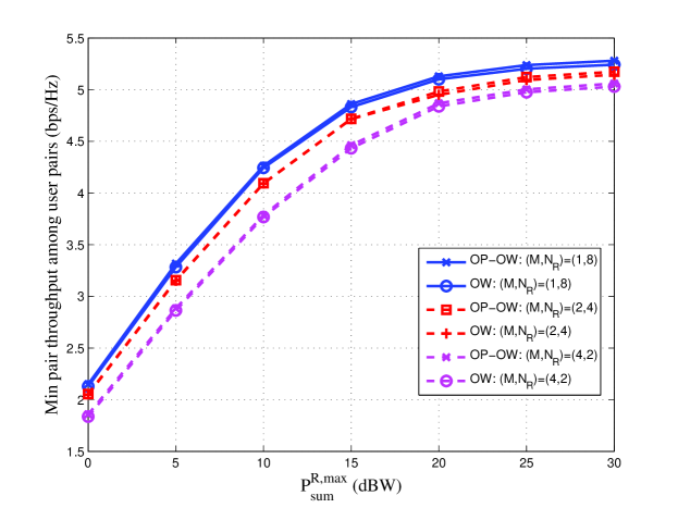
Figure 2: Minimum pair throughput among user pairs versus the relay power budget with $K=1$.

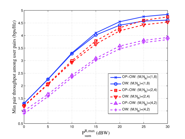
Figure 3: Minimum pair throughput among user pairs versus the relay power budget with $K=2$.

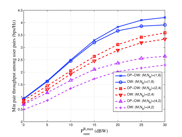
Figure 4: Minimum pair throughput among user pairs versus the relay power budget with $K=3$.

Table I provides the average number of iterations of Algorithm 1. As can be observed, Algorithm 1 converges in less than $24$ iterations in all considered scenarios.

TABLE I: Average number of iterations of Algorithm 1 with $K=2$.

$P_{\mathrm{sum}}^{R,\max}$ (dBW)	0	5	10	15	20	25	30
$(K,M,N_{R})=(2,1,8)$	15.47	12.02	9.72	8.05	11.10	18.45	15.60
$(K,M,N_{R})=(2,2,4)$	24.20	11.80	8.47	7.07	10.70	11.22	13.17
$(K,M,N_{R})=(2,4,2)$	22.47	22.95	13.72	12.07	7.90	10.40	11.97

V-B EE maximization

This subsection examines the performance of energy efficiency achieved by Algorithm 2. $r_{k}$ in (39) is set as the half of the optimal value obtained by Algorithm 1. Firstly, the simulation results presented in Fig. 5, 6 and 7 are for $K=2$ and $(M,N_{R})\in\{(1,8),(2,4),(4,2)\}$. Fig. 5 compares the EE performance achieved by TWR, one-way relaying and TWR with UE fixed equal power allocation, which is labelled as ”other method”. It is clear from Fig. 5 that TWR clearly and significantly outperforms one-way relaying and TWR UE equal power allocation.

Under small transmit power regime, the power consumption in the denominator is dominated by the circuit power and the EE is maximized by maximizing the sum throughput in the numerator. As such all the EE, the sum throughput and transmit power increase in Fig. 5, 6 and 7 in the relay power budget $P_{\mathrm{sum}}^{R,\max}$.

However, under larger transmit power regime, where the denominator of EE is dominated by the actual transmit power, the EE becomes to be maximized by minimizing the transmit power in the denominator, which saturates when beyond a threshold. When the transmit power saturates in Fig. 7, both the EE and the sum throughput accordingly saturate in Fig. 5 and 6. It is also observed that for a given relay power budget and a given number of total antennas in all relays, the configuration with less relays is superior to the ones with more relays. This is quite expected since the configuration with less relays achieves higher throughput than the ones with more relays. Table II shows that Algorithm 2 converges in less than $26$ iterations.

Similar comparisons are provided in Fig. 8 and 9 for $K=1$ and $K=3$, respectively with the superior EE performances of TWR over one-way relaying and TWR UE equal power allocation observed.

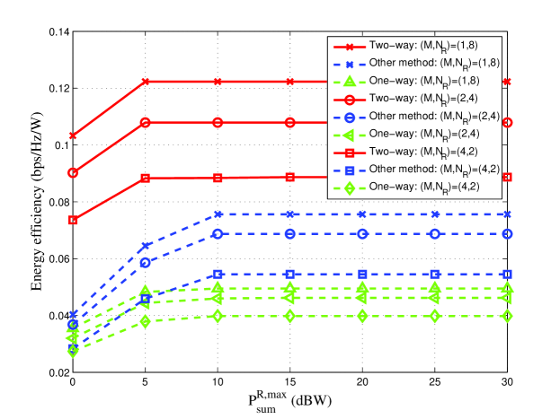
Figure 5: Energy efficiency versus the relay power budget with $K=2$

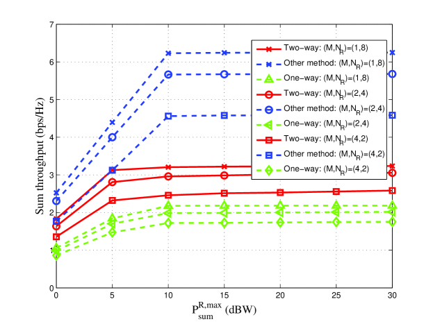
Figure 6: Sum rate versus the relay power budget with $K=2$

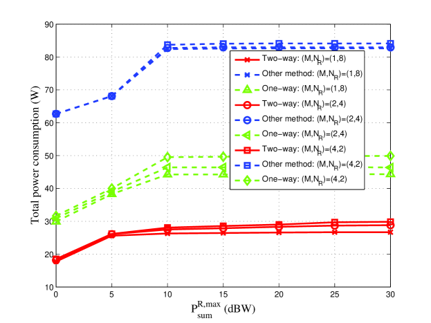
Figure 7: Total power versus the relay power budget with $K=2$

TABLE II: Average number of iterations of the proposed algorithm 2 for two-way with $K=2$.

$P_{\mathrm{sum}}^{R,\max}$ (dBW)	0	5	10	15	20	25	30
$(K,M,N_{R})=(2,1,8)$	23.21	23.08	5.85	12.65	14.06	14.98	15.53
$(K,M,N_{R})=(2,2,4)$	20.78	26.05	6.85	13.75	19.73	19.98	20.45
$(K,M,N_{R})=(2,4,2)$	21.11	22.95	8.03	9.61	17.41	19.96	21.46

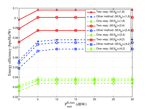
Figure 8: Energy efficiency versus the relay power budget with $K=1$

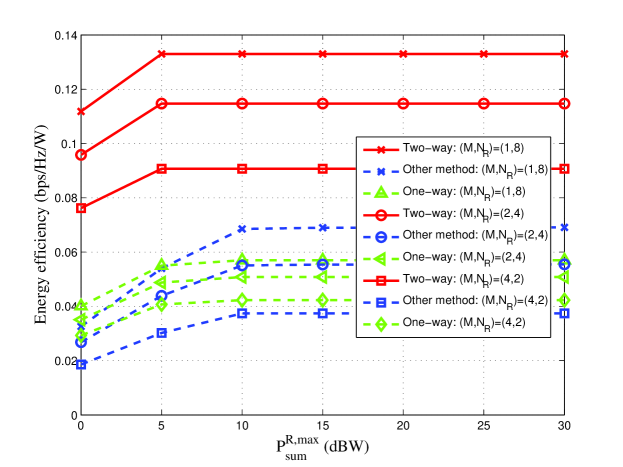
Figure 9: Energy efficiency versus the relay power budget with $K=3$

VI Conclusions

Joint UE power allocation and relay beamforming to either satisfy a UE’s QoS requirement or maximize the energy efficiency of TWR serving multiple UEs is a very difficult nonconvex optimization problem. This paper has developed two path-following computational procedures for their solutions, which invoke a simple convex quadratic program of low computational complexity at each iteration. Simulation results have confirmed their rapid convergence. We have shown that TWR achieves much higher energy-efficiency than its one-way relaying counterpart in all considered scenarios.

Appendix: proof for inequalities (27), (28) and (IV)

The function $\psi_{1}(z)=\ln(1+z^{-1})$ is convex on the domain $z>0$ [34]. Therefore [12]

$$\psi_{1}(z)\geq\psi(\bar{z})+\nabla\psi_{1}(\bar{z})(z-\bar{z})\ \quad\forall\ z>0,\bar{z}>0,$$

which is seen as

$$\ln(1+z^{-1})\geq\ln(1+\bar{z}^{-1})+\frac{1}{\bar{z}+1}-\frac{z}{(\bar{z}+1)\bar{z}}\quad\forall z>0,\bar{z}>0.$$ (46)

The inequality (27) is obtained by substituting $x=z^{-1}$ and $\bar{x}=\bar{z}^{-1}$ into (46).

Next, the function $\psi_{2}(x,\alpha,\beta)=|x|^{2}/\sqrt{\alpha\beta}$ is convex on the domain $z\in\mathbb{C},\alpha>0$ and $\beta>0$ [31], so again

$$\psi_{2}(x,\alpha,\beta)\geq\psi_{2}(\bar{x},\bar{\alpha},\bar{\beta})+\langle\nabla\psi_{2}(\bar{x},\bar{\alpha},\bar{\beta}),(x,\alpha,\beta)-(\bar{x},\bar{\alpha},\bar{\beta})\rangle,$$

which is seen as (28).

Finally, by checking its Hessian, the function $\psi_{3}(z,t)=(\ln(1+z^{-1}))/t$ is seen to be convex on the interior of ${\cal R}^{2}_{+}$. Therefore,

$$\psi_{3}(z,t)\geq\psi_{2}(\bar{z},\bar{t})+\langle\nabla\psi_{3}(\bar{z},\bar{t}),(z,t)-(\bar{z},\bar{t})\rangle\quad\forall\ z>0,\bar{z}>0,t>0,\bar{t}>0,$$

which is seen as

$$\frac{\ln(1+z^{-1})}{t}\geq 2\frac{\ln(1+\bar{z}^{-1})}{\bar{t}}+\frac{1}{(\bar{z}+1)\bar{t}}-\frac{z}{(\bar{z}+1)\bar{z}\bar{t}}-\frac{\ln(1+\bar{z})}{\bar{t}^{2}}t.$$

The inequality (IV) follows by substituting $x=z^{-1}$ and $\bar{x}=\bar{z}^{-1}$ into the last inequality.

References

• [1] G. Amarasuriya, C. Tellambura, and M. Ardakani, “Two-way amplify-and-forward multiple-input multiple-output relay networks with antenna selection,” IEEE J. Sel. Areas Commun., vol. 30, pp. 1513–1529, Sep. 2012.
• [2] H. Chung, N. Lee, B. Shim, and T. Oh, “On the beamforming design for MIMO multipair two-way relay channels,” IEEE Trans. Vehicular Technology, vol. 16, pp. 3301–3306, Sep. 2012.
• [3] D. Gunduz, A. Yener, A. Goldsmith, and H. V. Poor, “The multiway relay channel,” IEEE Trans. Inf. Theory, vol. 59, pp. 51–63, Jan 2013.
• [4] A. Asadi, Q. Wang, and V. Mancuso, “A survey device-to-device communication in cellular networks,” IEEE Commun. Surveys & Tut., vol. 16, pp. 1801–1819, 4th Qart. 2014.
• [5] J. Liu, N. Kato, J. Ma, and N. Kadowaki, “Device-to-device communication in LTE-advanced networks: A survey,” IEEE Commun. Surveys Tuts., vol. 17, pp. 1923–1940, 4th Quart. 2015.
• [6] R. Zhang, Y.-C. Liang, C. C. Chai, and S. Cui, “Optimal beamforming for two-way multi-antenna relay channel with analogue network coding,” IEEE J. Sel. Areas Commun., vol. 27, pp. 699–712, Jul. 2009.
• [7] M. Zeng, R. Zhang, and S. Cui, “On design of collaborative beamforming for two-way relay networks,” IEEE Trans. Signal Prosess., vol. 59, pp. 2284–2295, May 2011.
• [8] B. K. Chalise and L. Vandendorpe, “Optimization of MIMO relays for multipoint-to-multipoint communications: Nonrobust and robust designs,” IEEE Trans. Signal Prosess., vol. 58, pp. 6355–6368, Dec. 2010.
• [9] A. H. Phan, H. D. Tuan, H. H. Kha, and H. H. Nguyen, “Iterative D.C. optimization of precoding in wireless MIMO relaying,” IEEE Trans. Wireless Commun., vol. 12, pp. 1617–1627, Apr. 2013.
• [10] W. Cheng, M. Ghogho, Q. Huang, D. Ma, and J. Wei, “Maximizing the sum-rate of amplify-and-forward two-way relaying networks,” IEEE Signal Prosess. Lett., vol. 18, pp. 635–638, Nov. 2011.
• [11] M. Zaeri-Amirani, S. Shahbazpanahi, T. Mirfakhraie, and K. Ozdemir, “Performance tradeoffs in amplify-and-forward bidirectional network beamforming,” IEEE Trans. Signal Prosess., vol. 60, pp. 4196–7209, Aug. 2012.
• [12] H. Tuy, Convex Analysis and Global Optimization (second edition). Springer, 2016.
• [13] J. Zhang, F. Roemer, M. Haardt, A. Khabbazibasmenj, and S. A. Vorobyov, “Sum rate maximixation for multi-pair two-way relaying single-antenna amplify and forward relays,” in Proc. IEEE Int. Conf. Acoust Speech Signal Prosess. (ICASSP), Mar. 2012.
• [14] M. Tao and R. Wang, “Linear precoding for multi-pair two-way MIMO relay systems with max-min fairness,” IEEE Trans. Signal Prosess., vol. 60, pp. 5361–5370, Oct. 2012.
• [15] R. Wang, M. Tao, and Y. Huang, “Linear precoding designs for amplify-and-forward multiuser two-way relay systems,” IEEE Trans. Wireless Commun., vol. 11, pp. 4457–4469, Dec. 2012.
• [16] A. Khabbazibasmenj, F. Roemer, S. A. Vorobyov, and M. Haardt, “Sum-rate maximization in two-way AF MIMO relaying: Polynomial time solutions to a class of DC programming problems,” IEEE Trans. Signal Prosess., vol. 60, pp. 5478–5493, Dec. 2012.
• [17] M. R. A. Khandaker and Y. Rong, “Joint power control and beamforming for peer-to-peer MIMO relay systems,” in Proc. IEEE Int. Conf. Wireless Commun. Signal Prosess. (WCSP), Nov. 2011.
• [18] Y. Cheng and M. Pesavento, “Joint optimization of source power allocation and distributed relay beamforming in multiuser peer-to-peer relay networks,” IEEE Trans. Signal Prosess., vol. 60, pp. 2962–2973, Jun. 2012.
• [19] Y. Jing and S. Shahbazpanahi, “Max-min optimal joint power control and distributed beamforming for two-way relay networks under per-node power constraints,” IEEE Trans. Signal Prosess., vol. 60, pp. 6576–6589, Dec. 2012.
• [20] U. Rashid, H. D. Tuan, H. H. Kha, and H. H. Nguyen, “Joint optimization of source precoding and relay beamforming in wireless MIMO relay networks,” IEEE Trans. Commun., vol. 62, no. 2, pp. 488–499, 2014.
• [21] H. H. Kha, H. D. Tuan, H. H. Nguyen, and H. H. M. Tam, “Joint design of user power allocation and relay beamforming in two-way mimo relay networks,” in Proc. 7th Inter. Conf. Signal Process. Commun. Syst. (ICSPCS), pp. 1–6, 2013.
• [22] H. D. Tuan, D. T. Ngo, and H. H. M. Tam, “Joint power allocation for MIMO-OFDM full-duplex relaying communications,” EURASIP J. Wireless Commun. Networking, 2017, DOI 10.1186/s13638-016-0800-4.
• [23] E. Bjornson, E. A. Jorswieck, M. Debbah, and B. Ottersten, “Multiobjective signal processing optimization: The way to balance conflicting metrics in 5G systems,” IEEE Signal Process. Mag., vol. 31, pp. 14–23, Nov. 2014.
• [24] A. Fehske, G. Fettweis, J. Malmodin, and G. Biczok, “The global footprint of mobile communications: The ecological and economic perspective,” IEEE Commun. Mag., vol. 49, pp. 55–72, Aug. 2011.
• [25] S. Buzzi, C.-L. I, T. E. Klein, H. V. Poor, C. Yang, and A. Zappone, “A survey of energy-efficient techniques for 5G networks and challenges ahead,” IEEE J. Select. Areas Commun., vol. 34, pp. 697–709, Apr. 2016.
• [26] C. Xiong, L. Lu, and G. Y. Li, “Energy-efficient OFDMA-based two-way relay,” IEEE Trans. Commun., vol. 63, pp. 3157–3169, Sep. 2015.
• [27] J. Zhang and M. Haardt, “Energy efficient two-way non-regenerative relaying for relays with multiple antennas,” IEEE Signal Process. Lett., vol. 22, pp. 1079–1083, Aug. 2015.
• [28] Z. Wang, L. Li, H. Tian, and A. Paulraj, “User-centric precoding designs for the non-regenerative MIMO two-way relay systems,” IEEE Commun. Lett., vol. 20, pp. 1935–1938, Oct. 2016.
• [29] A. H. Phan, H. D. Tuan, H. H. Kha, and D. T. Ngo, “Nonsmooth optimization for efficient beamforming in cognitive radio multicast transmission,” IEEE Trans. Signal Process., vol. 60, pp. 2941–2951, Jun. 2012.
• [30] H. H. Kha, H. D. Tuan, and H. H. Nguyen, “Fast global optimal power allocation in wireless networks by local D.C. programming,” IEEE Trans. on Wireless Commun., vol. 1, pp. 510–515, Feb. 2012.
• [31] B. Dacorogna and P. Marechal, “The role of perspective functions in convexity, polyconvexity, rank-one convexity and separate convexity,” J. of Convex Analysis, vol. 15, no. 2, pp. 271–284, 2008.
• [32] H. H. M. Tam, H. D. Tuan, and D. T. Ngo, “Successive convex quadratic programming for quality-of-service management in full-duplex MU-MIMO multicell networks,” IEEE Trans. Comm., vol. 64, pp. 2340–2353, Jun. 2016.
• [33] C. Xiong, G. Y. Li, S. Zhang, Y. Chen, and S. Xu, “Energy-efficient resource allocation in OFDMA networks,” IEEE Trans. Commun., vol. 60, pp. 3767–3778, Dec. 2012.
• [34] H. M. T. Ho, H. D. Tuan, D. Ngo, T. Q. Duong, and V. Poor, “Joint load balancing and interference management for small-cell heterogeneous networks with limited backhaul capacity,” IEEE Trans. Wireless Commun., vol. PP, no. 99, pp. 1–1, 2016.