The Gaussian Stiffness of Graphene
deduced from a Continuum Model
based on Molecular Dynamics Potentials

Abstract

We consider a discrete model of a graphene sheet with atomic interactions governed by a harmonic approximation of the 2nd-generation Brenner potential that depends on bond lengths, bond angles, and two types of dihedral angles. A continuum limit is then deduced that fully describes the bending behavior. In particular, we deduce for the first time an analytical expression of the Gaussian stiffness, a scarcely investigated parameter ruling the rippling of graphene, for which contradictory values have been proposed in the literature. We disclose the atomic-scale sources of both bending and Gaussian stiffnesses and provide for them quantitative evaluations.

Keywords: Graphene, Continuum Modeling, Gaussian stiffness.

Contents

1. 1 Introduction
2. 2 Description of kinematics and energetics of the graphene sheet
3. 3 Approximated strain measures
   1. 3.1 Change of the edge lengths
   2. 3.2 Change of the wedge angles
   3. 3.3 Change of the dihedral angles
4. 4 Splitting of the energy
5. 5 The continuum limit
6. 6 The equivalent plate equation
7. 7 Numerical results
8. 8 Conclusions
9. A Appendix
   1. A.1 Change of the bond angle
   2. A.2 Change of the dihedral angle
   3. A.3 Deduction of the continuum limits $\mathcal{U}^{\mathcal{C}}_{0}$ and $\mathcal{U}^{(s)}_{0}$

1 Introduction

Graphene has attracted increasing interest during the past few years, and is nowadays used in a great variety of applications, taking advantage of its extraordinary mechanical, electrical and thermal conductivity properties. Nevertheless, its potentialities, and those of graphene-based materials, are far from being fully explored and exploited, and many studies are carried out by the scientific community in order to develop new technological applications [17].

The understanding of the bending behavior of graphene is of paramount importance in several technological applications. It is exploited, for example, to predict the performance of graphene nano-electro-mechanical devices and ripple formation [21, 28, 41, 25, 35, 22, 34, 20, 19, 38, 30, 15], and it is proposed to be the key point to produce efficient hydrogen-storage devices [36, 18, 37]. A very recent review in Materials Today by Deng & Berry [12] gives an overview on the hot problem of wrinkling, rippling and crumpling of graphene, highlighting formation mechanism and applications. Indeed, these corrugations can modify its electronic structure, create polarized carrier puddles, induce pseudo-magnetic field in bilayers and alter surface properties. Although a great effort has been done on the experimental side, predictive models are still wanted. They are of crucial importance when these phenomena need to be controlled and designed.

In particular, since the bending stiffness and the Gaussian stiffness —that is the reluctance to form non-null Gaussian curvatures— are the two crucial parameters governing the rippling of graphene, it is necessary to accurately determine them for both the design and the manipulation of graphene morphology. Although several evaluations of the bending stiffness have been proposed in the literature, the Gaussian stiffness has not been object of an intensive study. Indeed, as pointed out in a very recent review on mechanical properties of graphene [1], only two conflicting evaluations have been proposed. In [23], periodic boundary conditions have been used within a quantum-mechanical framework, and the value $-0.7$ eV has been found. While in [38] the estimate of $-1.52$ eV has been obtained by combining the configurational energy of membranes determined by Helfrich Hamiltonian with energies of fullerenes and single wall carbon nanotubes calculated by Density Functional Theory (DFT). At a discrete level there are two main difficulties in the evaluation of the Gaussian stiffness: on the one hand, controlling a discrete double curvature surfaces is problematic, and on the other hand, a suitable notion of Gaussian curvature at the discrete level should be introduced. Instead, when well established continuum models are adopted, such as plate theory, one has the problem of determining the equivalent stiffnesses, letting alone the conceptual crux of giving a meaning to the notion of thickness (see [21], [5] and references therein).

In this paper we deduce a continuum 2-dimensional model of a graphene sheet inferred from Molecular Dynamics (MD). In particular, looking at the 2nd-generation reactive empirical bond-order (REBO) potential [6], we give a nano-scale description of the atomic interactions and then we deduce the continuum limit, avoiding the problem of postulating an “equivalent thickness” and circumventing artificial procedures to identify the material parameters that describe the mechanical response of a plate within the classical theory.

Our analysis of the atomic-scale interaction relies on the discrete mechanical model proposed in [14] and exploited in [16, 15, 2], whose results are also based on the 2nd-generation Brenner potential. This potential is largely used in MD simulations for carbon allotropes; for a detailed description of its general form and that adopted in our theory we refer the reader to Appendix B of [14]. Here, we recall the key ingredients needed:

1. the kinematic variables associated with the interatomic bonds involve first, second and third nearest neighbors of any given atom. In particular, the kinematical variables we consider are bond lengths, bond angles, and dihedral angles; from [6] it results that these latter are of two kinds, that we here term C and Z, as carefully described in Sec. 2.

2. graphene suffers an angular self-stress, and the self-energy associated with the self-stress (sometimes called cohesive energy in the literature) is quantitatively relevant;

3. the energetic contribution of dihedral interaction is very relevant in bending.

For the first time, we propose a continuum model able to predict both the bending and the Gaussian stiffnesses. The analytical formula we obtain for the former predicts exactly the same value as that computed with MD simulations of the last generation. The value of the Gaussian stiffness we obtain is in very good agreement with DFT computations proposed in [38].

For the modeling of graphene many different approaches at different scales can be found in the literature, ranging from first principle calculations [24, 26], atomistic calculations [40, 42, 31] and continuum mechanics [7, 39, 29, 33, 32, 9, 8]. Furthermore, mixed atomistic formulations with finite elements have been reported for graphene [3, 4].

The paper is organized as follows. In Sec. 2, we describe the kinematics and the energetic of the graphene sheet at the nano-scale. In Sec. 3, we deduce the strain measures for the change of edge lengths, wedge angles and dihedral angles, approximated to the lowest order that makes the energy quadratic in the displacement. In Sec. 4, the total energy is split in its in-plane and out-of-plane contributions, and focus is set on the latter, having the first already been considered in [10]. In Sec. 5, we deduce a continuous energy that approximates the discrete energy and in Sec. 6 the limit energy is rearranged in a more amenable form, able to put in evidence the equivalence with plate theory. In Sec. 7, quantitative results for the continuum material parameters are deduced, by means of the 2nd-generation Brenner potential, and compared with the literature. Appendix A, containing some computations ancillary to Sec. 3, completes the paper.

2 Description of kinematics and energetics of the graphene sheet

At the nano-scale a graphene sheet is a discrete set of carbon atoms that, in the absence of external forces, sit at the vertices of a periodic array of hexagonal cells. More specifically, atoms occupy the nodes of the $2$–lattice, see Figure 1, generated by two simple Bravais lattices

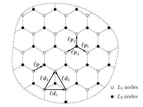
Figure 1: The hexagonal lattice

$$\begin{array}[]{l}L_{1}(\ell)=\{\mathbf{x}\in\mathbb{R}^{2}:\mathbf{x}=n^{1}\ell\mathbf{d}_{1}+n^{2}\ell\mathbf{d}_{2}\quad\mbox{with}\quad(n^{1},n^{2})\in\mathbb{Z}^{2}\},\\ L_{2}(\ell)=\ell\mathbf{p}+L_{1}(\ell),\end{array}$$ (1)

simply shifted with respect to one another. In (1), $\ell$ denotes the lattice size (the reference interatomic distance), while $\ell\mathbf{d}_{{{}\mathchoice{\mbox{\boldmath$\displaystyle\mathchar 267\relax$}}{\mbox{\boldmath$\textstyle\mathchar 267\relax$}}{\mbox{\boldmath$\scriptstyle\mathchar 267\relax$}}{\mbox{\boldmath$\scriptscriptstyle\mathchar 267\relax$}}}}$ and $\ell\mathbf{p}$ respectively are the lattice vectors and the shift vector, whose Cartesian components are given by

$$\mathbf{d}_{1}=(\sqrt{3},0),\quad\mathbf{d}_{2}=(\frac{\sqrt{3}}{2},\frac{3}{2})\quad\mbox{and}\quad\mathbf{p}=(\frac{\sqrt{3}}{2},\frac{1}{2}).$$ (2)

The sides of the hexagonal cells in Figure 1 stand for the bonds between pairs of next nearest neighbor atoms and are represented by the vectors

$$\mathbf{p}_{{}\mathchoice{\mbox{\boldmath$\displaystyle\mathchar 267\relax$}}{\mbox{\boldmath$\textstyle\mathchar 267\relax$}}{\mbox{\boldmath$\scriptstyle\mathchar 267\relax$}}{\mbox{\boldmath$\scriptscriptstyle\mathchar 267\relax$}}}=\mathbf{d}_{{}\mathchoice{\mbox{\boldmath$\displaystyle\mathchar 267\relax$}}{\mbox{\boldmath$\textstyle\mathchar 267\relax$}}{\mbox{\boldmath$\scriptstyle\mathchar 267\relax$}}{\mbox{\boldmath$\scriptscriptstyle\mathchar 267\relax$}}}-\mathbf{p}\ \ ({{}\mathchoice{\mbox{\boldmath$\displaystyle\mathchar 267\relax$}}{\mbox{\boldmath$\textstyle\mathchar 267\relax$}}{\mbox{\boldmath$\scriptstyle\mathchar 267\relax$}}{\mbox{\boldmath$\scriptscriptstyle\mathchar 267\relax$}}}=1,2)\quad\mbox{and}\quad\mathbf{p}_{3}=-\,\mathbf{p}.$$ (3)

For convenience we also set

$$\mathbf{d}_{3}=\mathbf{d}_{2}-\mathbf{d}_{1}.$$

As reference configuration we take the set of points $\mathbf{x}^{\ell}\in L^{1}(\ell)\cup L^{2}(\ell)$ contained in a bounded open set $\Omega\subset\mathbb{R}^{2}$.

Graphene mechanics is ruled by the interactions between the carbon atoms given by some suitable potential. According to the 2nd-generation Brenner potential [6], as detailed in [14, 16], in order to account properly for the mechanical behavior of a bended graphene sheet it is necessary to consider three types of energetic contributions, respectively coming from: binary interactions between next nearest atoms (edge bonds), three-bodies interactions between consecutive pairs of next nearest atoms (wedge bonds) and four-bodies interactions between three consecutive pairs of next nearest atoms (dihedral bonds). There are two types of relevant dihedral bonds: the Z-dihedra in which the edges connecting the four atoms form a z-shape and the C-dihedra in which the edges form a c-shape (see Fig. 2).

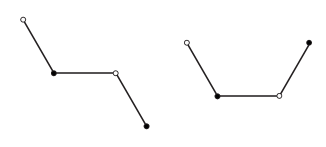
Figure 2: A Z-dihedral angle (left) and a C-dihedral angle (right).

We consider a harmonic approximation of the stored energy and assume that it is given by the sum of the following terms:

$$\begin{array}[]{l}\displaystyle\mathcal{U}_{\ell}^{l}=\frac{1}{2}\,\sum_{\mathcal{E}}k^{l}\,(l-l^{\mbox{\scriptsize nat}})^{2},\\ \displaystyle\mathcal{U}_{\ell}^{{}\mathchoice{\mbox{\boldmath$\displaystyle\mathchar 291\relax$}}{\mbox{\boldmath$\textstyle\mathchar 291\relax$}}{\mbox{\boldmath$\scriptstyle\mathchar 291\relax$}}{\mbox{\boldmath$\scriptscriptstyle\mathchar 291\relax$}}}=\frac{1}{2}\,\sum_{\mathcal{W}}k^{{}\mathchoice{\mbox{\boldmath$\displaystyle\mathchar 291\relax$}}{\mbox{\boldmath$\textstyle\mathchar 291\relax$}}{\mbox{\boldmath$\scriptstyle\mathchar 291\relax$}}{\mbox{\boldmath$\scriptscriptstyle\mathchar 291\relax$}}}\,({{}\mathchoice{\mbox{\boldmath$\displaystyle\mathchar 291\relax$}}{\mbox{\boldmath$\textstyle\mathchar 291\relax$}}{\mbox{\boldmath$\scriptstyle\mathchar 291\relax$}}{\mbox{\boldmath$\scriptscriptstyle\mathchar 291\relax$}}}\,-\,{{}\mathchoice{\mbox{\boldmath$\displaystyle\mathchar 291\relax$}}{\mbox{\boldmath$\textstyle\mathchar 291\relax$}}{\mbox{\boldmath$\scriptstyle\mathchar 291\relax$}}{\mbox{\boldmath$\scriptscriptstyle\mathchar 291\relax$}}}^{\mbox{\scriptsize nat}})^{2},\\ \displaystyle\mathcal{U}_{\ell}^{\Theta}=\frac{1}{2}\,\sum_{\mathcal{Z}}k^{\mathcal{Z}}\,(\operatorname{\overset{(z)}{\Theta}}\,-\,\Theta^{\mbox{\scriptsize nat}})^{2}+\frac{1}{2}\,\sum_{\mathcal{C}}k^{\mathcal{C}}\,(\operatorname{\overset{(c)}{\Theta}}\,-\,\Theta^{\mbox{\scriptsize nat}})^{2}\end{array}$$ (4)

$\mathcal{U}_{\ell}^{l}$, $\mathcal{U}_{\ell}^{{}\mathchoice{\mbox{\boldmath$\displaystyle\mathchar 291\relax$}}{\mbox{\boldmath$\textstyle\mathchar 291\relax$}}{\mbox{\boldmath$\scriptstyle\mathchar 291\relax$}}{\mbox{\boldmath$\scriptscriptstyle\mathchar 291\relax$}}}$ and $\mathcal{U}_{\ell}^{\Theta}$ are the energies of the edge bonds, the wedge bonds and the dihedral bonds, respectively; $l$ denotes the distance between nearest neighbor atoms, $\textstyle\mathchar 291\relax$ the angle between pairs of edges having a lattice point in common and $\operatorname{\overset{(z)}{\Theta}}$ and $\operatorname{\overset{(c)}{\Theta}}$ the Z- and C-dihedral angles between two consecutive wedges, to be defined later (see Fig. 3); $l^{\mbox{\scriptsize nat}}$ is the edge length at ease, ${{}\mathchoice{\mbox{\boldmath$\displaystyle\mathchar 291\relax$}}{\mbox{\boldmath$\textstyle\mathchar 291\relax$}}{\mbox{\boldmath$\scriptstyle\mathchar 291\relax$}}{\mbox{\boldmath$\scriptscriptstyle\mathchar 291\relax$}}}^{\mbox{\scriptsize nat}}$ the angle at ease between consecutive edges and $\Theta^{\mbox{\scriptsize nat}}$ the dihedral angle at ease.

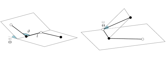
Figure 3: Kinematic variables: distance $l$, angle $\textstyle\mathchar 291\relax$, Z-dihedral angle $\operatorname{\overset{(z)}{\Theta}}$ and C-dihedral angle $\operatorname{\overset{(c)}{\Theta}}$.

The sums extend to all edges, $\mathcal{E}$, all wedges, $\mathcal{W}$, all Z-dihedra, $\mathcal{Z}$, and all C-dihedra, $\mathcal{C}$, contained in the set $\Omega$. The bond constants $k^{l}$, $k^{{}\mathchoice{\mbox{\boldmath$\displaystyle\mathchar 291\relax$}}{\mbox{\boldmath$\textstyle\mathchar 291\relax$}}{\mbox{\boldmath$\scriptstyle\mathchar 291\relax$}}{\mbox{\boldmath$\scriptscriptstyle\mathchar 291\relax$}}}$, $k^{\mathcal{Z}}$, and $k^{\mathcal{C}}$ will be deduced by making use of the 2nd-generation Brenner potential.

The graphene sheet does not have a configuration at ease (i.e. stress-free). Indeed, in [14] it has been shown that

$$\Theta^{\mbox{\scriptsize nat}}=0,\quad l^{\mbox{\scriptsize nat}}=\ell\quad\mbox{and}\quad{{}\mathchoice{\mbox{\boldmath$\displaystyle\mathchar 291\relax$}}{\mbox{\boldmath$\textstyle\mathchar 291\relax$}}{\mbox{\boldmath$\scriptstyle\mathchar 291\relax$}}{\mbox{\boldmath$\scriptscriptstyle\mathchar 291\relax$}}}^{\mbox{\scriptsize nat}}=\frac{2}{3}{{}\mathchoice{\mbox{\boldmath$\displaystyle\mathchar 281\relax$}}{\mbox{\boldmath$\textstyle\mathchar 281\relax$}}{\mbox{\boldmath$\scriptstyle\mathchar 281\relax$}}{\mbox{\boldmath$\scriptscriptstyle\mathchar 281\relax$}}}+{{}\mathchoice{\mbox{\boldmath$\displaystyle\mathchar 270\relax$}}{\mbox{\boldmath$\textstyle\mathchar 270\relax$}}{\mbox{\boldmath$\scriptstyle\mathchar 270\relax$}}{\mbox{\boldmath$\scriptscriptstyle\mathchar 270\relax$}}}{{}\mathchoice{\mbox{\boldmath$\displaystyle\mathchar 291\relax$}}{\mbox{\boldmath$\textstyle\mathchar 291\relax$}}{\mbox{\boldmath$\scriptstyle\mathchar 291\relax$}}{\mbox{\boldmath$\scriptscriptstyle\mathchar 291\relax$}}}_{0},$$

where ${{}\mathchoice{\mbox{\boldmath$\displaystyle\mathchar 270\relax$}}{\mbox{\boldmath$\textstyle\mathchar 270\relax$}}{\mbox{\boldmath$\scriptstyle\mathchar 270\relax$}}{\mbox{\boldmath$\scriptscriptstyle\mathchar 270\relax$}}}{{}\mathchoice{\mbox{\boldmath$\displaystyle\mathchar 291\relax$}}{\mbox{\boldmath$\textstyle\mathchar 291\relax$}}{\mbox{\boldmath$\scriptstyle\mathchar 291\relax$}}{\mbox{\boldmath$\scriptscriptstyle\mathchar 291\relax$}}}_{0}\neq 0$. We set ${{}\mathchoice{\mbox{\boldmath$\displaystyle\mathchar 270\relax$}}{\mbox{\boldmath$\textstyle\mathchar 270\relax$}}{\mbox{\boldmath$\scriptstyle\mathchar 270\relax$}}{\mbox{\boldmath$\scriptscriptstyle\mathchar 270\relax$}}}\Theta:=\Theta$, $l=\ell+{{}\mathchoice{\mbox{\boldmath$\displaystyle\mathchar 270\relax$}}{\mbox{\boldmath$\textstyle\mathchar 270\relax$}}{\mbox{\boldmath$\scriptstyle\mathchar 270\relax$}}{\mbox{\boldmath$\scriptscriptstyle\mathchar 270\relax$}}}l$ and ${{}\mathchoice{\mbox{\boldmath$\displaystyle\mathchar 291\relax$}}{\mbox{\boldmath$\textstyle\mathchar 291\relax$}}{\mbox{\boldmath$\scriptstyle\mathchar 291\relax$}}{\mbox{\boldmath$\scriptscriptstyle\mathchar 291\relax$}}}=\frac{2}{3}{{}\mathchoice{\mbox{\boldmath$\displaystyle\mathchar 281\relax$}}{\mbox{\boldmath$\textstyle\mathchar 281\relax$}}{\mbox{\boldmath$\scriptstyle\mathchar 281\relax$}}{\mbox{\boldmath$\scriptscriptstyle\mathchar 281\relax$}}}+{{}\mathchoice{\mbox{\boldmath$\displaystyle\mathchar 270\relax$}}{\mbox{\boldmath$\textstyle\mathchar 270\relax$}}{\mbox{\boldmath$\scriptstyle\mathchar 270\relax$}}{\mbox{\boldmath$\scriptscriptstyle\mathchar 270\relax$}}}{{}\mathchoice{\mbox{\boldmath$\displaystyle\mathchar 291\relax$}}{\mbox{\boldmath$\textstyle\mathchar 291\relax$}}{\mbox{\boldmath$\scriptstyle\mathchar 291\relax$}}{\mbox{\boldmath$\scriptscriptstyle\mathchar 291\relax$}}}$ and write (4) as

$$\begin{array}[]{l}\displaystyle\mathcal{U}_{\ell}^{l}=\frac{1}{2}\,\sum_{\mathcal{E}}k^{l}\,({{}\mathchoice{\mbox{\boldmath$\displaystyle\mathchar 270\relax$}}{\mbox{\boldmath$\textstyle\mathchar 270\relax$}}{\mbox{\boldmath$\scriptstyle\mathchar 270\relax$}}{\mbox{\boldmath$\scriptscriptstyle\mathchar 270\relax$}}}l)^{2},\\ \displaystyle\mathcal{U}_{\ell}^{{}\mathchoice{\mbox{\boldmath$\displaystyle\mathchar 291\relax$}}{\mbox{\boldmath$\textstyle\mathchar 291\relax$}}{\mbox{\boldmath$\scriptstyle\mathchar 291\relax$}}{\mbox{\boldmath$\scriptscriptstyle\mathchar 291\relax$}}}=\frac{1}{2}\,\sum_{\mathcal{W}}k^{{}\mathchoice{\mbox{\boldmath$\displaystyle\mathchar 291\relax$}}{\mbox{\boldmath$\textstyle\mathchar 291\relax$}}{\mbox{\boldmath$\scriptstyle\mathchar 291\relax$}}{\mbox{\boldmath$\scriptscriptstyle\mathchar 291\relax$}}}\,({{}\mathchoice{\mbox{\boldmath$\displaystyle\mathchar 270\relax$}}{\mbox{\boldmath$\textstyle\mathchar 270\relax$}}{\mbox{\boldmath$\scriptstyle\mathchar 270\relax$}}{\mbox{\boldmath$\scriptscriptstyle\mathchar 270\relax$}}}{{}\mathchoice{\mbox{\boldmath$\displaystyle\mathchar 291\relax$}}{\mbox{\boldmath$\textstyle\mathchar 291\relax$}}{\mbox{\boldmath$\scriptstyle\mathchar 291\relax$}}{\mbox{\boldmath$\scriptscriptstyle\mathchar 291\relax$}}}\,-\,{{}\mathchoice{\mbox{\boldmath$\displaystyle\mathchar 270\relax$}}{\mbox{\boldmath$\textstyle\mathchar 270\relax$}}{\mbox{\boldmath$\scriptstyle\mathchar 270\relax$}}{\mbox{\boldmath$\scriptscriptstyle\mathchar 270\relax$}}}{{}\mathchoice{\mbox{\boldmath$\displaystyle\mathchar 291\relax$}}{\mbox{\boldmath$\textstyle\mathchar 291\relax$}}{\mbox{\boldmath$\scriptstyle\mathchar 291\relax$}}{\mbox{\boldmath$\scriptscriptstyle\mathchar 291\relax$}}}_{0})^{2},\\ \displaystyle\mathcal{U}_{\ell}^{\Theta}=\frac{1}{2}\,\sum_{\mathcal{Z}}k^{\mathcal{Z}}\,({{}\mathchoice{\mbox{\boldmath$\displaystyle\mathchar 270\relax$}}{\mbox{\boldmath$\textstyle\mathchar 270\relax$}}{\mbox{\boldmath$\scriptstyle\mathchar 270\relax$}}{\mbox{\boldmath$\scriptscriptstyle\mathchar 270\relax$}}}\operatorname{\overset{(z)}{\Theta}})^{2}+\frac{1}{2}\,\sum_{\mathcal{C}}k^{\mathcal{C}}\,({{}\mathchoice{\mbox{\boldmath$\displaystyle\mathchar 270\relax$}}{\mbox{\boldmath$\textstyle\mathchar 270\relax$}}{\mbox{\boldmath$\scriptstyle\mathchar 270\relax$}}{\mbox{\boldmath$\scriptscriptstyle\mathchar 270\relax$}}}\operatorname{\overset{(c)}{\Theta}})^{2}\end{array}$$ (5)

In particular, up to a constant, the wedge energy takes the form

$$\mathcal{U}_{\ell}^{{}\mathchoice{\mbox{\boldmath$\displaystyle\mathchar 291\relax$}}{\mbox{\boldmath$\textstyle\mathchar 291\relax$}}{\mbox{\boldmath$\scriptstyle\mathchar 291\relax$}}{\mbox{\boldmath$\scriptscriptstyle\mathchar 291\relax$}}}={{}\mathchoice{\mbox{\boldmath$\displaystyle\mathchar 284\relax$}}{\mbox{\boldmath$\textstyle\mathchar 284\relax$}}{\mbox{\boldmath$\scriptstyle\mathchar 284\relax$}}{\mbox{\boldmath$\scriptscriptstyle\mathchar 284\relax$}}}_{0}\sum_{\mathcal{W}}{{}\mathchoice{\mbox{\boldmath$\displaystyle\mathchar 270\relax$}}{\mbox{\boldmath$\textstyle\mathchar 270\relax$}}{\mbox{\boldmath$\scriptstyle\mathchar 270\relax$}}{\mbox{\boldmath$\scriptscriptstyle\mathchar 270\relax$}}}{{}\mathchoice{\mbox{\boldmath$\displaystyle\mathchar 291\relax$}}{\mbox{\boldmath$\textstyle\mathchar 291\relax$}}{\mbox{\boldmath$\scriptstyle\mathchar 291\relax$}}{\mbox{\boldmath$\scriptscriptstyle\mathchar 291\relax$}}}+\frac{1}{2}\,\sum_{\mathcal{W}}k^{{}\mathchoice{\mbox{\boldmath$\displaystyle\mathchar 291\relax$}}{\mbox{\boldmath$\textstyle\mathchar 291\relax$}}{\mbox{\boldmath$\scriptstyle\mathchar 291\relax$}}{\mbox{\boldmath$\scriptscriptstyle\mathchar 291\relax$}}}\,({{}\mathchoice{\mbox{\boldmath$\displaystyle\mathchar 270\relax$}}{\mbox{\boldmath$\textstyle\mathchar 270\relax$}}{\mbox{\boldmath$\scriptstyle\mathchar 270\relax$}}{\mbox{\boldmath$\scriptscriptstyle\mathchar 270\relax$}}}{{}\mathchoice{\mbox{\boldmath$\displaystyle\mathchar 291\relax$}}{\mbox{\boldmath$\textstyle\mathchar 291\relax$}}{\mbox{\boldmath$\scriptstyle\mathchar 291\relax$}}{\mbox{\boldmath$\scriptscriptstyle\mathchar 291\relax$}}})^{2},$$ (6)

with

$${{}\mathchoice{\mbox{\boldmath$\displaystyle\mathchar 284\relax$}}{\mbox{\boldmath$\textstyle\mathchar 284\relax$}}{\mbox{\boldmath$\scriptstyle\mathchar 284\relax$}}{\mbox{\boldmath$\scriptscriptstyle\mathchar 284\relax$}}}_{0}:=-k^{{}\mathchoice{\mbox{\boldmath$\displaystyle\mathchar 291\relax$}}{\mbox{\boldmath$\textstyle\mathchar 291\relax$}}{\mbox{\boldmath$\scriptstyle\mathchar 291\relax$}}{\mbox{\boldmath$\scriptscriptstyle\mathchar 291\relax$}}}\,{{}\mathchoice{\mbox{\boldmath$\displaystyle\mathchar 270\relax$}}{\mbox{\boldmath$\textstyle\mathchar 270\relax$}}{\mbox{\boldmath$\scriptstyle\mathchar 270\relax$}}{\mbox{\boldmath$\scriptscriptstyle\mathchar 270\relax$}}}{{}\mathchoice{\mbox{\boldmath$\displaystyle\mathchar 291\relax$}}{\mbox{\boldmath$\textstyle\mathchar 291\relax$}}{\mbox{\boldmath$\scriptstyle\mathchar 291\relax$}}{\mbox{\boldmath$\scriptscriptstyle\mathchar 291\relax$}}}_{0}$$ (7)

the angle self-stress. The dihedral bonds play an important role because they contribute to the stored energy by about 50%, see [14, 15], the rest is due to the angle self-stress ${{}\mathchoice{\mbox{\boldmath$\displaystyle\mathchar 284\relax$}}{\mbox{\boldmath$\textstyle\mathchar 284\relax$}}{\mbox{\boldmath$\scriptstyle\mathchar 284\relax$}}{\mbox{\boldmath$\scriptscriptstyle\mathchar 284\relax$}}}_{0}$ associated to the wedge bonds.

The energy decomposition (5) is based on the choice of the set of kinematical variables $\{l,{{}\mathchoice{\mbox{\boldmath$\displaystyle\mathchar 291\relax$}}{\mbox{\boldmath$\textstyle\mathchar 291\relax$}}{\mbox{\boldmath$\scriptstyle\mathchar 291\relax$}}{\mbox{\boldmath$\scriptscriptstyle\mathchar 291\relax$}}},\operatorname{\overset{(z)}{\Theta}},\operatorname{\overset{(c)}{\Theta}}\}$. This choice is the most natural, if one considers the 2nd-generation Brenner potential, where all those variables appear in explicit manner. A harmonic approximation in each of those parameters is of course unique.

In the next section we shall make explicit the change of length ${{}\mathchoice{\mbox{\boldmath$\displaystyle\mathchar 270\relax$}}{\mbox{\boldmath$\textstyle\mathchar 270\relax$}}{\mbox{\boldmath$\scriptstyle\mathchar 270\relax$}}{\mbox{\boldmath$\scriptscriptstyle\mathchar 270\relax$}}}l$, the change of wedge angle $\textstyle\mathchar 270\relax$$\textstyle\mathchar 291\relax$, and the changes of the Z- and C-dihedral angles ${{}\mathchoice{\mbox{\boldmath$\displaystyle\mathchar 270\relax$}}{\mbox{\boldmath$\textstyle\mathchar 270\relax$}}{\mbox{\boldmath$\scriptstyle\mathchar 270\relax$}}{\mbox{\boldmath$\scriptscriptstyle\mathchar 270\relax$}}}\operatorname{\overset{(z)}{\Theta}}$ and ${{}\mathchoice{\mbox{\boldmath$\displaystyle\mathchar 270\relax$}}{\mbox{\boldmath$\textstyle\mathchar 270\relax$}}{\mbox{\boldmath$\scriptstyle\mathchar 270\relax$}}{\mbox{\boldmath$\scriptscriptstyle\mathchar 270\relax$}}}\operatorname{\overset{(c)}{\Theta}}$. In Section 4, with the notation introduced in the next section, we shall write the energies (5) more explicitly.

3 Approximated strain measures

In this section we calculate the strain measures associated to a change of configuration described by a displacement field $\mathbf{u}:(L_{1}(\ell)\cup L_{2}(\ell))\cap\Omega\to\mathbb{R}^{3}$, approximated to the lowest order that makes the energy quadratic in $\mathbf{u}$.

3.1 Change of the edge lengths

With ${{}\mathchoice{\mbox{\boldmath$\displaystyle\mathchar 270\relax$}}{\mbox{\boldmath$\textstyle\mathchar 270\relax$}}{\mbox{\boldmath$\scriptstyle\mathchar 270\relax$}}{\mbox{\boldmath$\scriptscriptstyle\mathchar 270\relax$}}}l_{i}(\mathbf{x}^{\ell})$ we denote the change in length of the edge parallel to $\mathbf{p}_{i}$ and starting from the lattice point $\mathbf{x}^{\ell}\in(L_{1}(\ell)\cup L_{2}(\ell))\cap\Omega$. Thus,

$${{}\mathchoice{\mbox{\boldmath$\displaystyle\mathchar 270\relax$}}{\mbox{\boldmath$\textstyle\mathchar 270\relax$}}{\mbox{\boldmath$\scriptstyle\mathchar 270\relax$}}{\mbox{\boldmath$\scriptscriptstyle\mathchar 270\relax$}}}l_{i}(\mathbf{x}^{\ell}) =|(\mathbf{x}^{\ell}+\ell\mathbf{p}_{i}+\mathbf{u}(\mathbf{x}^{\ell}+\ell\mathbf{p}_{i}))-(\mathbf{x}^{\ell}+\mathbf{u}(\mathbf{x}^{\ell}))|-\ell$$

$$=|\ell\mathbf{p}_{i}+(\mathbf{u}(\mathbf{x}^{\ell}+\ell\mathbf{p}_{i})-\mathbf{u}(\mathbf{x}^{\ell}))|-\ell,$$

and up to terms $o(|\mathbf{u}|)$ can be rewritten as

$${{}\mathchoice{\mbox{\boldmath$\displaystyle\mathchar 270\relax$}}{\mbox{\boldmath$\textstyle\mathchar 270\relax$}}{\mbox{\boldmath$\scriptstyle\mathchar 270\relax$}}{\mbox{\boldmath$\scriptscriptstyle\mathchar 270\relax$}}}l_{i}(\mathbf{x}^{\ell})=\frac{1}{\ell}\,(\mathbf{u}(\mathbf{x}^{\ell}+\ell\mathbf{p}_{i})-\mathbf{u}(\mathbf{x}^{\ell}))\cdot\mathbf{p}_{i}\qquad i=1,2,3.$$ (8)

In particular, the first order changes are determined by the in-plane components of $\mathbf{u}$ only.

3.2 Change of the wedge angles

For each fixed node $\mathbf{x}^{\ell}\in(L_{1}(\ell)\cup L_{2}(\ell))\cap\Omega$ we denote by ${{}\mathchoice{\mbox{\boldmath$\displaystyle\mathchar 291\relax$}}{\mbox{\boldmath$\textstyle\mathchar 291\relax$}}{\mbox{\boldmath$\scriptstyle\mathchar 291\relax$}}{\mbox{\boldmath$\scriptscriptstyle\mathchar 291\relax$}}}_{i}(\mathbf{x}^{\ell})$ the angle of the wedge delimited by the edges $\mathbf{p}_{i+1}$ and $\mathbf{p}_{i+2}$; that is, the wedge angle opposite to the $i$-th edge (see Fig. 4). Here, $i,i+1$, and $i+2$ take values in $\{1,2,3\}$ and the sums should be interpreted mod 3: for instance, if $i=2$ then $i+1=3$ and $i+2=1$.

Figure 4: The wedge angles ${{}\mathchoice{\mbox{\boldmath$\displaystyle\mathchar 291\relax$}}{\mbox{\boldmath$\textstyle\mathchar 291\relax$}}{\mbox{\boldmath$\scriptstyle\mathchar 291\relax$}}{\mbox{\boldmath$\scriptscriptstyle\mathchar 291\relax$}}}_{i}$.

From (6) we see that the change in the wedge angle enters into the energy not just quadratically but also linearly, therefore the variations of the wedge angle should be computed up to the second order approximation. To keep the notation compact, we set

$$\mathbf{u}_{i}:=\mathbf{u}(\mathbf{x}^{\ell}+\ell\mathbf{p}_{i}),\quad\mbox{and}\quad\mathbf{u}_{0}:=\mathbf{u}(\mathbf{x}^{\ell}).$$

Let

$$\mathbf{q}_{i+1} :=(\mathbf{x}^{\ell}+\ell\mathbf{p}_{i+1}+\mathbf{u}(\mathbf{x}^{\ell}+\ell\mathbf{p}_{i+1}))-(\mathbf{x}^{\ell}+\mathbf{u}(\mathbf{x}^{\ell}))$$

$$=\ell\mathbf{p}_{i+1}+(\mathbf{u}_{i+1}-\mathbf{u}_{0}),$$

and

$$\mathbf{q}_{i+2} :=(\mathbf{x}^{\ell}+\ell\mathbf{p}_{i+2}+\mathbf{u}(\mathbf{x}^{\ell}+\ell\mathbf{p}_{i+2}))-(\mathbf{x}^{\ell}+\mathbf{u}(\mathbf{x}^{\ell}))$$

$$=\ell\mathbf{p}_{i+2}+(\mathbf{u}_{i+2}-\mathbf{u}_{0}),$$

be the images of the edges parallel to $\mathbf{p}_{i+1}$ and $\mathbf{p}_{i+2}$ and starting at $\mathbf{x}^{\ell}$. Then, the angle ${{}\mathchoice{\mbox{\boldmath$\displaystyle\mathchar 291\relax$}}{\mbox{\boldmath$\textstyle\mathchar 291\relax$}}{\mbox{\boldmath$\scriptstyle\mathchar 291\relax$}}{\mbox{\boldmath$\scriptscriptstyle\mathchar 291\relax$}}}_{i}={{}\mathchoice{\mbox{\boldmath$\displaystyle\mathchar 291\relax$}}{\mbox{\boldmath$\textstyle\mathchar 291\relax$}}{\mbox{\boldmath$\scriptstyle\mathchar 291\relax$}}{\mbox{\boldmath$\scriptscriptstyle\mathchar 291\relax$}}}_{i}(\mathbf{x}^{\ell})$ is given by

$$\cos({{}\mathchoice{\mbox{\boldmath$\displaystyle\mathchar 291\relax$}}{\mbox{\boldmath$\textstyle\mathchar 291\relax$}}{\mbox{\boldmath$\scriptstyle\mathchar 291\relax$}}{\mbox{\boldmath$\scriptscriptstyle\mathchar 291\relax$}}}_{i})=\frac{{\mathbf{q}_{i+1}}\cdot{\mathbf{q}_{i+2}}}{|{\mathbf{q}_{i+1}}||{\mathbf{q}_{i+2}}|}.$$ (9)

Calculations given in Appendix A.1 yield that

$${{}\mathchoice{\mbox{\boldmath$\displaystyle\mathchar 291\relax$}}{\mbox{\boldmath$\textstyle\mathchar 291\relax$}}{\mbox{\boldmath$\scriptstyle\mathchar 291\relax$}}{\mbox{\boldmath$\scriptscriptstyle\mathchar 291\relax$}}}_{i}=\frac{2}{3}{{}\mathchoice{\mbox{\boldmath$\displaystyle\mathchar 281\relax$}}{\mbox{\boldmath$\textstyle\mathchar 281\relax$}}{\mbox{\boldmath$\scriptstyle\mathchar 281\relax$}}{\mbox{\boldmath$\scriptscriptstyle\mathchar 281\relax$}}}+{{}\mathchoice{\mbox{\boldmath$\displaystyle\mathchar 270\relax$}}{\mbox{\boldmath$\textstyle\mathchar 270\relax$}}{\mbox{\boldmath$\scriptstyle\mathchar 270\relax$}}{\mbox{\boldmath$\scriptscriptstyle\mathchar 270\relax$}}}{{}\mathchoice{\mbox{\boldmath$\displaystyle\mathchar 291\relax$}}{\mbox{\boldmath$\textstyle\mathchar 291\relax$}}{\mbox{\boldmath$\scriptstyle\mathchar 291\relax$}}{\mbox{\boldmath$\scriptscriptstyle\mathchar 291\relax$}}}_{i}^{(1)}+{{}\mathchoice{\mbox{\boldmath$\displaystyle\mathchar 270\relax$}}{\mbox{\boldmath$\textstyle\mathchar 270\relax$}}{\mbox{\boldmath$\scriptstyle\mathchar 270\relax$}}{\mbox{\boldmath$\scriptscriptstyle\mathchar 270\relax$}}}{{}\mathchoice{\mbox{\boldmath$\displaystyle\mathchar 291\relax$}}{\mbox{\boldmath$\textstyle\mathchar 291\relax$}}{\mbox{\boldmath$\scriptstyle\mathchar 291\relax$}}{\mbox{\boldmath$\scriptscriptstyle\mathchar 291\relax$}}}_{i}^{(2)}+o(|\mathbf{u}|^{2}),$$ (10)

where ${{}\mathchoice{\mbox{\boldmath$\displaystyle\mathchar 270\relax$}}{\mbox{\boldmath$\textstyle\mathchar 270\relax$}}{\mbox{\boldmath$\scriptstyle\mathchar 270\relax$}}{\mbox{\boldmath$\scriptscriptstyle\mathchar 270\relax$}}}{{}\mathchoice{\mbox{\boldmath$\displaystyle\mathchar 291\relax$}}{\mbox{\boldmath$\textstyle\mathchar 291\relax$}}{\mbox{\boldmath$\scriptstyle\mathchar 291\relax$}}{\mbox{\boldmath$\scriptscriptstyle\mathchar 291\relax$}}}_{i}^{(1)}$ and ${{}\mathchoice{\mbox{\boldmath$\displaystyle\mathchar 270\relax$}}{\mbox{\boldmath$\textstyle\mathchar 270\relax$}}{\mbox{\boldmath$\scriptstyle\mathchar 270\relax$}}{\mbox{\boldmath$\scriptscriptstyle\mathchar 270\relax$}}}{{}\mathchoice{\mbox{\boldmath$\displaystyle\mathchar 291\relax$}}{\mbox{\boldmath$\textstyle\mathchar 291\relax$}}{\mbox{\boldmath$\scriptstyle\mathchar 291\relax$}}{\mbox{\boldmath$\scriptscriptstyle\mathchar 291\relax$}}}_{i}^{(2)}$ are the first order and the second order variation, respectively, of the wedge angle with respect to the reference angle $\frac{2}{3}{{}\mathchoice{\mbox{\boldmath$\displaystyle\mathchar 281\relax$}}{\mbox{\boldmath$\textstyle\mathchar 281\relax$}}{\mbox{\boldmath$\scriptstyle\mathchar 281\relax$}}{\mbox{\boldmath$\scriptscriptstyle\mathchar 281\relax$}}}$. Therefore, keeping up to second order terms one has that

$${{}\mathchoice{\mbox{\boldmath$\displaystyle\mathchar 270\relax$}}{\mbox{\boldmath$\textstyle\mathchar 270\relax$}}{\mbox{\boldmath$\scriptstyle\mathchar 270\relax$}}{\mbox{\boldmath$\scriptscriptstyle\mathchar 270\relax$}}}{{}\mathchoice{\mbox{\boldmath$\displaystyle\mathchar 291\relax$}}{\mbox{\boldmath$\textstyle\mathchar 291\relax$}}{\mbox{\boldmath$\scriptstyle\mathchar 291\relax$}}{\mbox{\boldmath$\scriptscriptstyle\mathchar 291\relax$}}}_{i}={{}\mathchoice{\mbox{\boldmath$\displaystyle\mathchar 270\relax$}}{\mbox{\boldmath$\textstyle\mathchar 270\relax$}}{\mbox{\boldmath$\scriptstyle\mathchar 270\relax$}}{\mbox{\boldmath$\scriptscriptstyle\mathchar 270\relax$}}}{{}\mathchoice{\mbox{\boldmath$\displaystyle\mathchar 291\relax$}}{\mbox{\boldmath$\textstyle\mathchar 291\relax$}}{\mbox{\boldmath$\scriptstyle\mathchar 291\relax$}}{\mbox{\boldmath$\scriptscriptstyle\mathchar 291\relax$}}}_{i}^{(1)}+{{}\mathchoice{\mbox{\boldmath$\displaystyle\mathchar 270\relax$}}{\mbox{\boldmath$\textstyle\mathchar 270\relax$}}{\mbox{\boldmath$\scriptstyle\mathchar 270\relax$}}{\mbox{\boldmath$\scriptscriptstyle\mathchar 270\relax$}}}{{}\mathchoice{\mbox{\boldmath$\displaystyle\mathchar 291\relax$}}{\mbox{\boldmath$\textstyle\mathchar 291\relax$}}{\mbox{\boldmath$\scriptstyle\mathchar 291\relax$}}{\mbox{\boldmath$\scriptscriptstyle\mathchar 291\relax$}}}_{i}^{(2)}.$$ (11)

It turns out that the first order variation takes the form

$${{}\mathchoice{\mbox{\boldmath$\displaystyle\mathchar 270\relax$}}{\mbox{\boldmath$\textstyle\mathchar 270\relax$}}{\mbox{\boldmath$\scriptstyle\mathchar 270\relax$}}{\mbox{\boldmath$\scriptscriptstyle\mathchar 270\relax$}}}{{}\mathchoice{\mbox{\boldmath$\displaystyle\mathchar 291\relax$}}{\mbox{\boldmath$\textstyle\mathchar 291\relax$}}{\mbox{\boldmath$\scriptstyle\mathchar 291\relax$}}{\mbox{\boldmath$\scriptscriptstyle\mathchar 291\relax$}}}_{i}^{(1)}(\mathbf{x}^{\ell})=-\frac{1}{\ell}(\mathbf{u}_{i+1}-\mathbf{u}_{0})\cdot\mathbf{p}_{i+1}^{\perp}+\frac{1}{\ell}(\mathbf{u}_{i+2}-\mathbf{u}_{0})\cdot\mathbf{p}_{i+2}^{\perp},$$ (12)

with $\mathbf{p}_{i+1}^{\perp}$ defined by

$$\mathbf{p}_{i+1}^{\perp}:=\frac{\mathbf{p}_{i+2}+\frac{1}{2}\mathbf{p}_{i+1}}{|\mathbf{p}_{i+2}+\frac{1}{2}\mathbf{p}_{i+1}|}=\frac{2}{\sqrt{3}}(\mathbf{p}_{i+2}+\frac{1}{2}\mathbf{p}_{i+1})\qquad i=1,2,3,$$ (13)

that is, the unit vector orthogonal to $\mathbf{p}_{i+1}$, (cf. equation (19) in [13]).

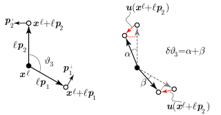
Figure 5: The first order approximation of the change in the wedge angle.

Figure 5 illustrates the geometrical meaning of formula (12). In particular,

$$\sum_{i=1}^{3}{{}\mathchoice{\mbox{\boldmath$\displaystyle\mathchar 270\relax$}}{\mbox{\boldmath$\textstyle\mathchar 270\relax$}}{\mbox{\boldmath$\scriptstyle\mathchar 270\relax$}}{\mbox{\boldmath$\scriptscriptstyle\mathchar 270\relax$}}}{{}\mathchoice{\mbox{\boldmath$\displaystyle\mathchar 291\relax$}}{\mbox{\boldmath$\textstyle\mathchar 291\relax$}}{\mbox{\boldmath$\scriptstyle\mathchar 291\relax$}}{\mbox{\boldmath$\scriptscriptstyle\mathchar 291\relax$}}}_{i}^{(1)}(\mathbf{x}^{\ell})=0,$$

as it could have been deduced from geometrical considerations.

The second order variation is given by, see Appendix A.1,

$${{}\mathchoice{\mbox{\boldmath$\displaystyle\mathchar 270\relax$}}{\mbox{\boldmath$\textstyle\mathchar 270\relax$}}{\mbox{\boldmath$\scriptstyle\mathchar 270\relax$}}{\mbox{\boldmath$\scriptscriptstyle\mathchar 270\relax$}}}{{}\mathchoice{\mbox{\boldmath$\displaystyle\mathchar 291\relax$}}{\mbox{\boldmath$\textstyle\mathchar 291\relax$}}{\mbox{\boldmath$\scriptstyle\mathchar 291\relax$}}{\mbox{\boldmath$\scriptscriptstyle\mathchar 291\relax$}}}_{i}^{(2)}(\mathbf{x}^{\ell})=-\frac{1}{\sqrt{3}}\Bigg{[} -\frac{1}{2}{({{}\mathchoice{\mbox{\boldmath$\displaystyle\mathchar 270\relax$}}{\mbox{\boldmath$\textstyle\mathchar 270\relax$}}{\mbox{\boldmath$\scriptstyle\mathchar 270\relax$}}{\mbox{\boldmath$\scriptscriptstyle\mathchar 270\relax$}}}{{}\mathchoice{\mbox{\boldmath$\displaystyle\mathchar 291\relax$}}{\mbox{\boldmath$\textstyle\mathchar 291\relax$}}{\mbox{\boldmath$\scriptstyle\mathchar 291\relax$}}{\mbox{\boldmath$\scriptscriptstyle\mathchar 291\relax$}}}_{i}^{(1)})}^{2}+\frac{2}{\ell^{2}}(\mathbf{u}_{i+1}-\mathbf{u}_{0})\cdot(\mathbf{u}_{i+2}-\mathbf{u}_{0})-$$ (14)

$$\left(\frac{(\mathbf{u}_{i+1}-\mathbf{u}_{0})}{\ell^{2}}\cdot\mathbf{p}_{i+1}+\frac{(\mathbf{u}_{i+2}-\mathbf{u}_{0})}{\ell^{2}}\cdot\mathbf{p}_{i+2}\right)\times$$

$$\times\left(\frac{(\mathbf{u}_{i+1}-\mathbf{u}_{0})}{\ell^{2}}\cdot\mathbf{p}_{i+2}+\frac{(\mathbf{u}_{i+2}-\mathbf{u}_{0})}{\ell^{2}}\cdot\mathbf{p}_{i+1}-\frac{\sqrt{3}}{2}{{}\mathchoice{\mbox{\boldmath$\displaystyle\mathchar 270\relax$}}{\mbox{\boldmath$\textstyle\mathchar 270\relax$}}{\mbox{\boldmath$\scriptstyle\mathchar 270\relax$}}{\mbox{\boldmath$\scriptscriptstyle\mathchar 270\relax$}}}{{}\mathchoice{\mbox{\boldmath$\displaystyle\mathchar 291\relax$}}{\mbox{\boldmath$\textstyle\mathchar 291\relax$}}{\mbox{\boldmath$\scriptstyle\mathchar 291\relax$}}{\mbox{\boldmath$\scriptscriptstyle\mathchar 291\relax$}}}_{i}^{(1)}\right)$$

$$-\frac{\mathbf{p}_{i+1}\cdot\mathbf{p}_{i+2}}{\ell^{4}}\Big{(}|\mathbf{u}_{i+1}-\mathbf{u}_{0}|^{2}-2\frac{1}{\ell^{2}}\big{(}\mathbf{p}_{i+1}\cdot(\mathbf{u}_{i+1}-\mathbf{u}_{0})\big{)}^{2}$$

$$+|\mathbf{u}_{i+2}-\mathbf{u}_{0}|^{2}-2\frac{1}{\ell^{2}}\big{(}\mathbf{p}_{i+2}\cdot(\mathbf{u}_{i+2}-\mathbf{u}_{0})\big{)}^{2}\Bigg{]}.$$

By algebric manipulation one finds that

$$\sum_{i=1}^{3}{{}\mathchoice{\mbox{\boldmath$\displaystyle\mathchar 270\relax$}}{\mbox{\boldmath$\textstyle\mathchar 270\relax$}}{\mbox{\boldmath$\scriptstyle\mathchar 270\relax$}}{\mbox{\boldmath$\scriptscriptstyle\mathchar 270\relax$}}}{{}\mathchoice{\mbox{\boldmath$\displaystyle\mathchar 291\relax$}}{\mbox{\boldmath$\textstyle\mathchar 291\relax$}}{\mbox{\boldmath$\scriptstyle\mathchar 291\relax$}}{\mbox{\boldmath$\scriptscriptstyle\mathchar 291\relax$}}}_{i}(\mathbf{x}^{\ell})=\sum_{i=1}^{3}{{}\mathchoice{\mbox{\boldmath$\displaystyle\mathchar 270\relax$}}{\mbox{\boldmath$\textstyle\mathchar 270\relax$}}{\mbox{\boldmath$\scriptstyle\mathchar 270\relax$}}{\mbox{\boldmath$\scriptscriptstyle\mathchar 270\relax$}}}{{}\mathchoice{\mbox{\boldmath$\displaystyle\mathchar 291\relax$}}{\mbox{\boldmath$\textstyle\mathchar 291\relax$}}{\mbox{\boldmath$\scriptstyle\mathchar 291\relax$}}{\mbox{\boldmath$\scriptscriptstyle\mathchar 291\relax$}}}_{i}^{(2)}(\mathbf{x}^{\ell})=-\frac{3\sqrt{3}}{\ell^{2}}\Bigg{(}\frac{1}{3}\sum_{i=1}^{3}w(\mathbf{x}^{\ell}+\ell\mathbf{p}_{i})-w(\mathbf{x}^{\ell})\Bigg{)}^{2},$$ (15)

where $w$ denotes the out-of-plane component of the displacement, that is

$$w:=\mathbf{u}\cdot\mathbf{e}_{3},$$

where $\mathbf{e}_{3}$ is the unit vector perpendicular to the undeformed sheet. Note that, by (15), the $\sum_{i}{{}\mathchoice{\mbox{\boldmath$\displaystyle\mathchar 270\relax$}}{\mbox{\boldmath$\textstyle\mathchar 270\relax$}}{\mbox{\boldmath$\scriptstyle\mathchar 270\relax$}}{\mbox{\boldmath$\scriptscriptstyle\mathchar 270\relax$}}}{{}\mathchoice{\mbox{\boldmath$\displaystyle\mathchar 291\relax$}}{\mbox{\boldmath$\textstyle\mathchar 291\relax$}}{\mbox{\boldmath$\scriptstyle\mathchar 291\relax$}}{\mbox{\boldmath$\scriptscriptstyle\mathchar 291\relax$}}}_{i}(\mathbf{x}^{\ell})$ is non-positive and hence the contribution of the self-stress to the strain energy is non-negative for ${{}\mathchoice{\mbox{\boldmath$\displaystyle\mathchar 284\relax$}}{\mbox{\boldmath$\textstyle\mathchar 284\relax$}}{\mbox{\boldmath$\scriptstyle\mathchar 284\relax$}}{\mbox{\boldmath$\scriptscriptstyle\mathchar 284\relax$}}}_{0}<0$, i.e., for ${{}\mathchoice{\mbox{\boldmath$\displaystyle\mathchar 270\relax$}}{\mbox{\boldmath$\textstyle\mathchar 270\relax$}}{\mbox{\boldmath$\scriptstyle\mathchar 270\relax$}}{\mbox{\boldmath$\scriptscriptstyle\mathchar 270\relax$}}}{{}\mathchoice{\mbox{\boldmath$\displaystyle\mathchar 291\relax$}}{\mbox{\boldmath$\textstyle\mathchar 291\relax$}}{\mbox{\boldmath$\scriptstyle\mathchar 291\relax$}}{\mbox{\boldmath$\scriptscriptstyle\mathchar 291\relax$}}}_{0}>0$, see (7).

3.3 Change of the dihedral angles

For each fixed node $\mathbf{x}^{\ell}\in L_{2}(\ell)\cap\Omega$ and for each edge parallel to $\mathbf{p}_{i}$ and starting at $\mathbf{x}^{\ell}$ we need to define four types of dihedral angles $\operatorname{\overset{(c)}{\Theta}}_{\mathbf{p}_{i}^{+}}(\mathbf{x}^{\ell}),\operatorname{\overset{(c)}{\Theta}}_{\mathbf{p}_{i}^{-}}(\mathbf{x}^{\ell}),\operatorname{\overset{(z)}{\Theta}}_{\mathbf{p}_{i}\mathbf{p}_{i+1}}(\mathbf{x}^{\ell})$ and $\operatorname{\overset{(z)}{\Theta}}_{\mathbf{p}_{i}\mathbf{p}_{i+2}}(\mathbf{x}^{\ell})$:

$$\cos\operatorname{\overset{(c)}{\Theta}}_{\mathbf{p}_{i}^{+}}=\frac{(\mathbf{q}_{i}\times\mathbf{q}_{i+1})\cdot(\mathbf{q}_{i}\times\mathbf{q}_{i^{+}})}{|\mathbf{q}_{i}\times\mathbf{q}_{i+1}||\mathbf{q}_{i}\times\mathbf{q}_{i^{+}}|},$$ (16)

$$\cos\operatorname{\overset{(c)}{\Theta}}_{\mathbf{p}_{i}^{-}}=\frac{(\mathbf{q}_{i+2}\times\mathbf{q}_{i})\cdot(\mathbf{q}_{i^{-}}\times\mathbf{q}_{i})}{|\mathbf{q}_{i+2}\times\mathbf{q}_{i}||\mathbf{q}_{i^{-}}\times\mathbf{q}_{i})|},$$

$$\cos\operatorname{\overset{(z)}{\Theta}}_{\mathbf{p}_{i}\mathbf{p}_{i+1}}=\frac{(\mathbf{q}_{i}\times\mathbf{q}_{i+1})\cdot(\mathbf{q}_{i^{-}}\times\mathbf{q}_{i})}{|\mathbf{q}_{i}\times\mathbf{q}_{i+1}||\mathbf{q}_{i^{-}}\times\mathbf{q}_{i}|},$$

$$\cos\operatorname{\overset{(z)}{\Theta}}_{\mathbf{p}_{i}\mathbf{p}_{i+2}}=\frac{(\mathbf{q}_{i+2}\times\mathbf{q}_{i})\cdot(\mathbf{q}_{i}\times\mathbf{q}_{i^{+}})}{|\mathbf{q}_{i+2}\times\mathbf{q}_{i}||\mathbf{q}_{i}\times\mathbf{q}_{i^{+}}|},$$

where

$$\mathbf{q}_{i^{+}}= \mathbf{x}^{\ell}+\ell\mathbf{p}_{i}-\ell\mathbf{p}_{i+2}+\mathbf{u}(\mathbf{x}^{\ell}+\ell\mathbf{p}_{i}-\ell\mathbf{p}_{i+2})-\big{(}\mathbf{x}^{\ell}+\ell\mathbf{p}_{i}+\mathbf{u}(\mathbf{x}^{\ell}+\ell\mathbf{p}_{i})\big{)}$$ (17)

$$= -\ell\mathbf{p}_{i+2}+\mathbf{u}_{i^{+}}-\mathbf{u}_{i},\qquad\qquad\mathbf{u}_{i^{+}}:=\mathbf{u}(\mathbf{x}^{\ell}+\ell\mathbf{p}_{i}-\ell\mathbf{p}_{i+2}),$$

$$\mathbf{q}_{i^{-}}= \mathbf{x}^{\ell}+\ell\mathbf{p}_{i}-\ell\mathbf{p}_{i+1}+\mathbf{u}(\mathbf{x}^{\ell}+\ell\mathbf{p}_{i}-\ell\mathbf{p}_{i+1})-\big{(}\mathbf{x}^{\ell}+\ell\mathbf{p}_{i}+\mathbf{u}(\mathbf{x}^{\ell}+\ell\mathbf{p}_{i})\big{)}$$

$$= -\ell\mathbf{p}_{i+1}+\mathbf{u}_{i^{-}}-\mathbf{u}_{i},\qquad\qquad\mathbf{u}_{i^{-}}:=\mathbf{u}(\mathbf{x}^{\ell}+\ell\mathbf{p}_{i}-\ell\mathbf{p}_{i+1})$$

are the images of vectors $\ell\mathbf{p}_{i^{+}}$ and $\ell\mathbf{p}_{i^{-}}$ (see Fig. 6, for $i=1$), parallel to $\mathbf{p}_{i+2}$ and $\mathbf{p}_{i+1}$ and starting at the image of the point $\mathbf{x}^{\ell}+\ell\mathbf{p}_{i}$.

Also here, $i,i+1$, and $i+2$ take values in $\{1,2,3\}$ and the sums should be interpreted mod 3: for instance, if $i=3$ then $i+1=1$ and $i+2=2$.

The C-dihedral angle $\operatorname{\overset{(c)}{\Theta}}_{\mathbf{p}_{i}^{+}}(\mathbf{x}^{\ell})$ is the angle corresponding to the C-dihedron with middle edge $\ell\mathbf{p}_{i}$ and oriented as $\mathbf{p}_{i}^{\perp}$, while $\operatorname{\overset{(c)}{\Theta}}_{\mathbf{p}_{i}^{-}}(\mathbf{x}^{\ell})$ is the angle corresponding to the C-dihedron oriented opposite to $\mathbf{p}_{i}^{\perp}$ (see Fig. 6 for $i=1$). The Z-dihedral angle $\operatorname{\overset{(z)}{\Theta}}_{\mathbf{p}_{i}\mathbf{p}_{i+1}}(\mathbf{x}^{\ell})$ corresponds to the Z-dihedron with middle edge $\ell\mathbf{p}_{i}$ and the other two edges parallel to $\mathbf{p}_{i+1}$ (see Fig. 6 for $i=1$).

Figure 6: Left: C-dihedral angles $\operatorname{\overset{(c)}{\Theta}}_{\mathbf{p}_{1}^{+}}$ (green) and Z-dihedral angle $\operatorname{\overset{(z)}{\Theta}}_{\mathbf{p}_{1}\mathbf{p}_{2}}$ (blue). Right: C-dihedral angles $\operatorname{\overset{(c)}{\Theta}}_{\mathbf{p}_{1}^{-}}$ (green) and Z-dihedral angle $\operatorname{\overset{(z)}{\Theta}}_{\mathbf{p}_{1}\mathbf{p}_{3}}$ (blue).

Then, recalling that ${{}\mathchoice{\mbox{\boldmath$\displaystyle\mathchar 270\relax$}}{\mbox{\boldmath$\textstyle\mathchar 270\relax$}}{\mbox{\boldmath$\scriptstyle\mathchar 270\relax$}}{\mbox{\boldmath$\scriptscriptstyle\mathchar 270\relax$}}}\Theta=\Theta$, calculations in Appendix A.2 yield that

$${{}\mathchoice{\mbox{\boldmath$\displaystyle\mathchar 270\relax$}}{\mbox{\boldmath$\textstyle\mathchar 270\relax$}}{\mbox{\boldmath$\scriptstyle\mathchar 270\relax$}}{\mbox{\boldmath$\scriptscriptstyle\mathchar 270\relax$}}}\operatorname{\overset{(c)}{\Theta}}_{\mathbf{p}_{i}^{+}}(\mathbf{x}^{\ell})=\frac{2\sqrt{3}}{3\ell}[2w(\mathbf{x}^{\ell})-w(\mathbf{x}^{\ell}+\ell\mathbf{p}_{i+1})+w(\mathbf{x}^{\ell}+\ell\mathbf{p}_{i}-\ell\mathbf{p}_{i+2})-2w(\mathbf{x}^{\ell}+\ell\mathbf{p}_{i})],$$ (18)

and

$${{}\mathchoice{\mbox{\boldmath$\displaystyle\mathchar 270\relax$}}{\mbox{\boldmath$\textstyle\mathchar 270\relax$}}{\mbox{\boldmath$\scriptstyle\mathchar 270\relax$}}{\mbox{\boldmath$\scriptscriptstyle\mathchar 270\relax$}}}\operatorname{\overset{(z)}{\Theta}}_{\mathbf{p}_{i}\mathbf{p}_{i+1}}(\mathbf{x}^{\ell})=\frac{2\sqrt{3}}{3\ell}[w(\mathbf{x}^{\ell}+\ell\mathbf{p}_{i}-\ell\mathbf{p}_{i+1})-w(\mathbf{x}^{\ell}+\ell\mathbf{p}_{i})+w(\mathbf{x}^{\ell}+\ell\mathbf{p}_{i+1})-w(\mathbf{x}^{\ell})].$$ (19)

Analogous formulas hold for ${{}\mathchoice{\mbox{\boldmath$\displaystyle\mathchar 270\relax$}}{\mbox{\boldmath$\textstyle\mathchar 270\relax$}}{\mbox{\boldmath$\scriptstyle\mathchar 270\relax$}}{\mbox{\boldmath$\scriptscriptstyle\mathchar 270\relax$}}}\operatorname{\overset{(c)}{\Theta}}_{\mathbf{p}_{i}^{-}}$ and ${{}\mathchoice{\mbox{\boldmath$\displaystyle\mathchar 270\relax$}}{\mbox{\boldmath$\textstyle\mathchar 270\relax$}}{\mbox{\boldmath$\scriptstyle\mathchar 270\relax$}}{\mbox{\boldmath$\scriptscriptstyle\mathchar 270\relax$}}}\operatorname{\overset{(z)}{\Theta}}_{\mathbf{p}_{i}\mathbf{p}_{i+2}}$:

$${{}\mathchoice{\mbox{\boldmath$\displaystyle\mathchar 270\relax$}}{\mbox{\boldmath$\textstyle\mathchar 270\relax$}}{\mbox{\boldmath$\scriptstyle\mathchar 270\relax$}}{\mbox{\boldmath$\scriptscriptstyle\mathchar 270\relax$}}}\operatorname{\overset{(c)}{\Theta}}_{\mathbf{p}_{i}^{-}}(\mathbf{x}^{\ell})=-\frac{2\sqrt{3}}{3\ell}[2w(\mathbf{x}^{\ell})-w(\mathbf{x}^{\ell}+\ell\mathbf{p}_{i+2})+w(\mathbf{x}^{\ell}+\ell\mathbf{p}_{i}-\ell\mathbf{p}_{i+1})-2w(\mathbf{x}^{\ell}+\ell\mathbf{p}_{i})],$$ (20)

$${{}\mathchoice{\mbox{\boldmath$\displaystyle\mathchar 270\relax$}}{\mbox{\boldmath$\textstyle\mathchar 270\relax$}}{\mbox{\boldmath$\scriptstyle\mathchar 270\relax$}}{\mbox{\boldmath$\scriptscriptstyle\mathchar 270\relax$}}}\operatorname{\overset{(z)}{\Theta}}_{\mathbf{p}_{i}\mathbf{p}_{i+2}}(\mathbf{x}^{\ell})=\frac{2\sqrt{3}}{3\ell}[w(\mathbf{x}^{\ell}+\ell\mathbf{p}_{i}-\ell\mathbf{p}_{i+2})-w(\mathbf{x}^{\ell}+\ell\mathbf{p}_{i})+w(\mathbf{x}^{\ell}+\ell\mathbf{p}_{i+2})-w(\mathbf{x}^{\ell})].$$

4 Splitting of the energy

The above calculations show that ${{}\mathchoice{\mbox{\boldmath$\displaystyle\mathchar 270\relax$}}{\mbox{\boldmath$\textstyle\mathchar 270\relax$}}{\mbox{\boldmath$\scriptstyle\mathchar 270\relax$}}{\mbox{\boldmath$\scriptscriptstyle\mathchar 270\relax$}}}{{}\mathchoice{\mbox{\boldmath$\displaystyle\mathchar 291\relax$}}{\mbox{\boldmath$\textstyle\mathchar 291\relax$}}{\mbox{\boldmath$\scriptstyle\mathchar 291\relax$}}{\mbox{\boldmath$\scriptscriptstyle\mathchar 291\relax$}}}_{i}^{(1)}$ as well as ${{}\mathchoice{\mbox{\boldmath$\displaystyle\mathchar 270\relax$}}{\mbox{\boldmath$\textstyle\mathchar 270\relax$}}{\mbox{\boldmath$\scriptstyle\mathchar 270\relax$}}{\mbox{\boldmath$\scriptscriptstyle\mathchar 270\relax$}}}l_{i}$ depend upon the in-plane components of $\mathbf{u}$, cf.  (8) and (12), while ${{}\mathchoice{\mbox{\boldmath$\displaystyle\mathchar 270\relax$}}{\mbox{\boldmath$\textstyle\mathchar 270\relax$}}{\mbox{\boldmath$\scriptstyle\mathchar 270\relax$}}{\mbox{\boldmath$\scriptscriptstyle\mathchar 270\relax$}}}{{}\mathchoice{\mbox{\boldmath$\displaystyle\mathchar 291\relax$}}{\mbox{\boldmath$\textstyle\mathchar 291\relax$}}{\mbox{\boldmath$\scriptstyle\mathchar 291\relax$}}{\mbox{\boldmath$\scriptscriptstyle\mathchar 291\relax$}}}_{i}^{(2)}$, ${{}\mathchoice{\mbox{\boldmath$\displaystyle\mathchar 270\relax$}}{\mbox{\boldmath$\textstyle\mathchar 270\relax$}}{\mbox{\boldmath$\scriptstyle\mathchar 270\relax$}}{\mbox{\boldmath$\scriptscriptstyle\mathchar 270\relax$}}}\operatorname{\overset{(c)}{\Theta}}$, and ${{}\mathchoice{\mbox{\boldmath$\displaystyle\mathchar 270\relax$}}{\mbox{\boldmath$\textstyle\mathchar 270\relax$}}{\mbox{\boldmath$\scriptstyle\mathchar 270\relax$}}{\mbox{\boldmath$\scriptscriptstyle\mathchar 270\relax$}}}\operatorname{\overset{(z)}{\Theta}}$ depend upon the out-of-plane component of $\mathbf{u}$, cf.  (15), (18), and (19). This yields a splitting of the energy into membrane and bending parts

$$\mathcal{U}_{\ell}=\mathcal{U}_{\ell}^{(m)}+\mathcal{U}_{\ell}^{(b)},\quad\mathcal{U}_{\ell}^{(b)}:=\mathcal{U}_{\ell}^{(s)}+\mathcal{U}_{\ell}^{(d)}$$

defined by

$$\mathcal{U}_{\ell}^{(m)}:=\frac{1}{2}\,\sum_{\mathcal{E}}k^{l}\,({{}\mathchoice{\mbox{\boldmath$\displaystyle\mathchar 270\relax$}}{\mbox{\boldmath$\textstyle\mathchar 270\relax$}}{\mbox{\boldmath$\scriptstyle\mathchar 270\relax$}}{\mbox{\boldmath$\scriptscriptstyle\mathchar 270\relax$}}}l)^{2}+\frac{1}{2}\,\sum_{\mathcal{W}}k^{{}\mathchoice{\mbox{\boldmath$\displaystyle\mathchar 291\relax$}}{\mbox{\boldmath$\textstyle\mathchar 291\relax$}}{\mbox{\boldmath$\scriptstyle\mathchar 291\relax$}}{\mbox{\boldmath$\scriptscriptstyle\mathchar 291\relax$}}}\,{({{}\mathchoice{\mbox{\boldmath$\displaystyle\mathchar 270\relax$}}{\mbox{\boldmath$\textstyle\mathchar 270\relax$}}{\mbox{\boldmath$\scriptstyle\mathchar 270\relax$}}{\mbox{\boldmath$\scriptscriptstyle\mathchar 270\relax$}}}{{}\mathchoice{\mbox{\boldmath$\displaystyle\mathchar 291\relax$}}{\mbox{\boldmath$\textstyle\mathchar 291\relax$}}{\mbox{\boldmath$\scriptstyle\mathchar 291\relax$}}{\mbox{\boldmath$\scriptscriptstyle\mathchar 291\relax$}}}^{(1)})}^{2}$$ (21)

$$\mathcal{U}_{\ell}^{(s)}:={{}\mathchoice{\mbox{\boldmath$\displaystyle\mathchar 284\relax$}}{\mbox{\boldmath$\textstyle\mathchar 284\relax$}}{\mbox{\boldmath$\scriptstyle\mathchar 284\relax$}}{\mbox{\boldmath$\scriptscriptstyle\mathchar 284\relax$}}}_{0}\sum_{\mathcal{W}}{{}\mathchoice{\mbox{\boldmath$\displaystyle\mathchar 270\relax$}}{\mbox{\boldmath$\textstyle\mathchar 270\relax$}}{\mbox{\boldmath$\scriptstyle\mathchar 270\relax$}}{\mbox{\boldmath$\scriptscriptstyle\mathchar 270\relax$}}}{{}\mathchoice{\mbox{\boldmath$\displaystyle\mathchar 291\relax$}}{\mbox{\boldmath$\textstyle\mathchar 291\relax$}}{\mbox{\boldmath$\scriptstyle\mathchar 291\relax$}}{\mbox{\boldmath$\scriptscriptstyle\mathchar 291\relax$}}}^{(2)},$$

$$\mathcal{U}_{\ell}^{(d)}:=\frac{1}{2}\,\sum_{\mathcal{Z}}k^{\mathcal{Z}}\,({{}\mathchoice{\mbox{\boldmath$\displaystyle\mathchar 270\relax$}}{\mbox{\boldmath$\textstyle\mathchar 270\relax$}}{\mbox{\boldmath$\scriptstyle\mathchar 270\relax$}}{\mbox{\boldmath$\scriptscriptstyle\mathchar 270\relax$}}}\operatorname{\overset{(z)}{\Theta}})^{2}+\frac{1}{2}\,\sum_{\mathcal{C}}k^{\mathcal{C}}\,({{}\mathchoice{\mbox{\boldmath$\displaystyle\mathchar 270\relax$}}{\mbox{\boldmath$\textstyle\mathchar 270\relax$}}{\mbox{\boldmath$\scriptstyle\mathchar 270\relax$}}{\mbox{\boldmath$\scriptscriptstyle\mathchar 270\relax$}}}\operatorname{\overset{(c)}{\Theta}})^{2},$$

where $\mathcal{U}_{\ell}^{(s)}$ is the self-energy (corresponding to the so-called cohesive energy in the literature) and $\mathcal{U}_{\ell}^{(d)}$ is the dihedral energy. The analysis in a paper by Davini [10] applies here to the in-plane deformations, providing a continuum model of the graphene sheet within the framework of $\Gamma$-convergence theory. Hereafter, we concentrate on the out-of-plane deformations. With the notation introduced in Section 3 we now write the bending energy more explicitly. The self-energy can be written as

$$\mathcal{U}^{(s)}_{\ell}=\sum_{\mathbf{x}^{\ell}\in(L_{1}(\ell)\cup L_{2}(\ell))\cap\Omega}{{}\mathchoice{\mbox{\boldmath$\displaystyle\mathchar 284\relax$}}{\mbox{\boldmath$\textstyle\mathchar 284\relax$}}{\mbox{\boldmath$\scriptstyle\mathchar 284\relax$}}{\mbox{\boldmath$\scriptscriptstyle\mathchar 284\relax$}}}_{0}\sum_{i=1}^{3}{{}\mathchoice{\mbox{\boldmath$\displaystyle\mathchar 270\relax$}}{\mbox{\boldmath$\textstyle\mathchar 270\relax$}}{\mbox{\boldmath$\scriptstyle\mathchar 270\relax$}}{\mbox{\boldmath$\scriptscriptstyle\mathchar 270\relax$}}}{{}\mathchoice{\mbox{\boldmath$\displaystyle\mathchar 291\relax$}}{\mbox{\boldmath$\textstyle\mathchar 291\relax$}}{\mbox{\boldmath$\scriptstyle\mathchar 291\relax$}}{\mbox{\boldmath$\scriptscriptstyle\mathchar 291\relax$}}}_{i}^{(2)}(\mathbf{x}^{\ell}),$$ (22)

where $\sum_{i=1}^{3}{{}\mathchoice{\mbox{\boldmath$\displaystyle\mathchar 270\relax$}}{\mbox{\boldmath$\textstyle\mathchar 270\relax$}}{\mbox{\boldmath$\scriptstyle\mathchar 270\relax$}}{\mbox{\boldmath$\scriptscriptstyle\mathchar 270\relax$}}}{{}\mathchoice{\mbox{\boldmath$\displaystyle\mathchar 291\relax$}}{\mbox{\boldmath$\textstyle\mathchar 291\relax$}}{\mbox{\boldmath$\scriptstyle\mathchar 291\relax$}}{\mbox{\boldmath$\scriptscriptstyle\mathchar 291\relax$}}}_{i}^{(2)}(\mathbf{x}^{\ell})$ is given in (15) in terms of the out-of-plane component of the displacement $w$. We further split the dihedral energy $\mathcal{U}_{\ell}^{(d)}$ in

$$\mathcal{U}_{\ell}^{(d)}:=\mathcal{U}^{\mathcal{Z}}_{\ell}+\mathcal{U}^{\mathcal{C}}_{\ell},$$

where

$$\mathcal{U}^{\mathcal{Z}}_{\ell}=\frac{1}{2}\,k^{\mathcal{Z}}\sum_{\mathbf{x}^{\ell}\in L_{2}(\ell)\cap\Omega}\sum_{i=1}^{3}\Bigg{(}{{}\mathchoice{\mbox{\boldmath$\displaystyle\mathchar 270\relax$}}{\mbox{\boldmath$\textstyle\mathchar 270\relax$}}{\mbox{\boldmath$\scriptstyle\mathchar 270\relax$}}{\mbox{\boldmath$\scriptscriptstyle\mathchar 270\relax$}}}\operatorname{\overset{(z)}{\Theta}}_{\mathbf{p}_{i}\mathbf{p}_{i+2}}(\mathbf{x}^{\ell})\Bigg{)}^{2}+\Bigg{(}{{}\mathchoice{\mbox{\boldmath$\displaystyle\mathchar 270\relax$}}{\mbox{\boldmath$\textstyle\mathchar 270\relax$}}{\mbox{\boldmath$\scriptstyle\mathchar 270\relax$}}{\mbox{\boldmath$\scriptscriptstyle\mathchar 270\relax$}}}\operatorname{\overset{(z)}{\Theta}}_{\mathbf{p}_{i}\mathbf{p}_{i+1}}(\mathbf{x}^{\ell})\Bigg{)}^{2}$$ (23)

is the contribution of the Z-dihedra, and

$$\mathcal{U}^{\mathcal{C}}_{\ell}=\frac{1}{2}k^{\mathcal{C}}\,\sum_{\mathbf{x}^{\ell}\in L_{2}(\ell)\cap\Omega}\sum_{i=1}^{3}\Bigg{(}{{}\mathchoice{\mbox{\boldmath$\displaystyle\mathchar 270\relax$}}{\mbox{\boldmath$\textstyle\mathchar 270\relax$}}{\mbox{\boldmath$\scriptstyle\mathchar 270\relax$}}{\mbox{\boldmath$\scriptscriptstyle\mathchar 270\relax$}}}\operatorname{\overset{(c)}{\Theta}}_{\mathbf{p}_{i}^{+}}(\mathbf{x}^{\ell})\Bigg{)}^{2}+\Bigg{(}{{}\mathchoice{\mbox{\boldmath$\displaystyle\mathchar 270\relax$}}{\mbox{\boldmath$\textstyle\mathchar 270\relax$}}{\mbox{\boldmath$\scriptstyle\mathchar 270\relax$}}{\mbox{\boldmath$\scriptscriptstyle\mathchar 270\relax$}}}\operatorname{\overset{(c)}{\Theta}}_{\mathbf{p}_{i}^{-}}(\mathbf{x}^{\ell})\Bigg{)}^{2}$$ (24)

is the contribution of the C-dihedra. The Z- and C-dihedral angles appearing in (38) and (37) are given in terms of $w$ in (18)-(20).

In the next section we deduce, by means of a formal analysis, a continuous version of the discrete bending energy

$$\mathcal{U}_{\ell}^{(b)}=\mathcal{U}_{\ell}^{(s)}+\mathcal{U}^{\mathcal{Z}}_{\ell}+\mathcal{U}^{\mathcal{C}}_{\ell},$$ (25)

from which we shall deduce expressions for the sheet’s bending stiffnesses. A rigorous analysis based on $\Gamma$-convergence theory will be done in a forthcoming paper [11].

5 The continuum limit

In this section we find a continuous energy, defined over the domain $\Omega$, that approximates the discrete bending energy $\mathcal{U}_{\ell}^{(b)}$ defined over the lattice $(L_{1}(\ell)\cup L_{2}(\ell))\cap\Omega$. This is achieved by letting the lattice size $\ell$ go to zero so that $(L_{1}(\ell)\cup L_{2}(\ell))\cap\Omega$ invades $\Omega$. With this in mind, in place of a function $w:(L_{1}(\ell)\cup L_{2}(\ell))\cap\Omega\to\mathbb{R}$, we consider a twice continuously differentiable function $w:\Omega\to\mathbb{R}$.

Given two vectors $\mathbf{a}$ and $\mathbf{b}$, with $\partial^{2}_{\mathbf{a}\mathbf{b}}w$ we denote the second partial derivative of $w$ in the directions $\mathbf{a}/|\mathbf{a}|$ and $\mathbf{b}/|\mathbf{b}|$, that is

$$\partial^{2}_{\mathbf{a}\mathbf{b}}w=\nabla^{2}w\frac{\mathbf{a}}{|\mathbf{a}|}\cdot\frac{\mathbf{b}}{|\mathbf{b}|},$$

where $\nabla^{2}w$ denotes the Hessian of $w$. Clearly, we also have

$$\partial^{2}_{\mathbf{a}\mathbf{b}}w(x_{0})=\lim_{\ell\to 0}\frac{w(x_{0}+\ell\mathbf{a}+\ell\mathbf{b})-w(x_{0}+\ell\mathbf{b})-w(x_{0}+\ell\mathbf{a})+w(x_{0})}{\ell^{2}|\mathbf{a}||\mathbf{b}|}.$$ (26)

The change of the Z-dihedra, see (20)₂, can be rewritten, after setting

$$\mathbf{a}_{i}:=\mathbf{p}_{i}-\mathbf{p}_{i+2},$$ (27)

as

$${{}\mathchoice{\mbox{\boldmath$\displaystyle\mathchar 270\relax$}}{\mbox{\boldmath$\textstyle\mathchar 270\relax$}}{\mbox{\boldmath$\scriptstyle\mathchar 270\relax$}}{\mbox{\boldmath$\scriptscriptstyle\mathchar 270\relax$}}}\operatorname{\overset{(z)}{\Theta}}_{\mathbf{p}_{i}\mathbf{p}_{i+2}}(\mathbf{x}^{\ell}) =\frac{2\sqrt{3}}{3\ell}[w(\mathbf{x}^{\ell}+\ell\mathbf{p}_{i}-\ell\mathbf{p}_{i+2})-w(\mathbf{x}^{\ell})-w(\mathbf{x}^{\ell}+\ell\mathbf{p}_{i})+w(\mathbf{x}^{\ell}+\ell\mathbf{p}_{i+2})]$$

$$=\frac{2\sqrt{3}}{3\ell}[w(\mathbf{x}^{\ell}+\ell\mathbf{a}_{i})-w(\mathbf{x}^{\ell})-w(\mathbf{x}^{\ell}+\ell\mathbf{a}_{i}+\ell\mathbf{p}_{i+2})+w(\mathbf{x}^{\ell}+\ell\mathbf{p}_{i+2})]$$

$$=\frac{2\sqrt{3}}{3\ell}[-\partial^{2}_{\mathbf{a}_{i}\mathbf{p}_{i+2}}w(\mathbf{x}^{\ell})\ell^{2}|\mathbf{a}_{i}||\mathbf{p}_{i+2}|+o(\ell^{2})]$$

$$=-2\ell\partial^{2}_{\mathbf{a}_{i}\mathbf{p}_{i+2}}w(\mathbf{x}^{\ell})+o(\ell),$$ (28)

where the third equality follows from (26). Similarly, setting

$$\mathbf{b}_{i}:=\mathbf{p}_{i}-\mathbf{p}_{i+1},$$ (29)

we have that

$${{}\mathchoice{\mbox{\boldmath$\displaystyle\mathchar 270\relax$}}{\mbox{\boldmath$\textstyle\mathchar 270\relax$}}{\mbox{\boldmath$\scriptstyle\mathchar 270\relax$}}{\mbox{\boldmath$\scriptscriptstyle\mathchar 270\relax$}}}\operatorname{\overset{(z)}{\Theta}}_{\mathbf{p}_{i}\mathbf{p}_{i+1}}(\mathbf{x}^{\ell}) =\frac{2\sqrt{3}}{3\ell}[w(\mathbf{x}^{\ell}+\ell\mathbf{p}_{i}-\ell\mathbf{p}_{i+1})-w(\mathbf{x}^{\ell}+\ell\mathbf{p}_{i})+w(\mathbf{x}^{\ell}+\ell\mathbf{p}_{i+1})-w(\mathbf{x}^{\ell})]$$

$$=\frac{2\sqrt{3}}{3\ell}[w(\mathbf{x}^{\ell}+\ell\mathbf{b}_{i})-w(\mathbf{x}^{\ell}+\ell\mathbf{b}_{i}+\ell\mathbf{p}_{i+1})+w(\mathbf{x}^{\ell}+\ell\mathbf{p}_{i+1})-w(\mathbf{x}^{\ell})]$$

$$=-2\ell\partial^{2}_{\mathbf{b}_{i}\mathbf{p}_{i+1}}w(\mathbf{x}^{\ell})+o(\ell).$$ (30)

Taking (3) into account, we may rewrite the vectors $\mathbf{a}_{i}$ and $\mathbf{b}_{i}$, defined in (27) and (29), in terms of $\mathbf{d}_{i}$, for instance $\mathbf{a}_{1}=\mathbf{d}_{1}$ and $\mathbf{b}_{1}=-\mathbf{d}_{3}$, and then rewrite the Z-dihedral energy, see (38) and rewritten below for the reader convenience, as

$$\mathcal{U}^{\mathcal{Z}}_{\ell} =\frac{1}{2}\,k^{\mathcal{Z}}\sum_{\mathbf{x}^{\ell}\in L_{2}(\ell)\cap\Omega}\sum_{i=1}^{3}\Bigg{(}{{}\mathchoice{\mbox{\boldmath$\displaystyle\mathchar 270\relax$}}{\mbox{\boldmath$\textstyle\mathchar 270\relax$}}{\mbox{\boldmath$\scriptstyle\mathchar 270\relax$}}{\mbox{\boldmath$\scriptscriptstyle\mathchar 270\relax$}}}\operatorname{\overset{(z)}{\Theta}}_{\mathbf{p}_{i}\mathbf{p}_{i+2}}(\mathbf{x}^{\ell})\Bigg{)}^{2}+\Bigg{(}{{}\mathchoice{\mbox{\boldmath$\displaystyle\mathchar 270\relax$}}{\mbox{\boldmath$\textstyle\mathchar 270\relax$}}{\mbox{\boldmath$\scriptstyle\mathchar 270\relax$}}{\mbox{\boldmath$\scriptscriptstyle\mathchar 270\relax$}}}\operatorname{\overset{(z)}{\Theta}}_{\mathbf{p}_{i}\mathbf{p}_{i+1}}(\mathbf{x}^{\ell})\Bigg{)}^{2}$$

$$=\frac{1}{2}{4}\ell^{2}k^{\mathcal{Z}}\sum_{\mathbf{x}^{\ell}\in L_{2}(\ell)\cap\Omega}(\partial^{2}_{\mathbf{d}_{1}\mathbf{p}_{3}}w(\mathbf{x}^{\ell}))^{2}+(\partial^{2}_{\mathbf{d}_{1}\mathbf{p}_{1}}w(\mathbf{x}^{\ell}))^{2}+(\partial^{2}_{\mathbf{d}_{2}\mathbf{p}_{2}}w(\mathbf{x}^{\ell}))^{2}$$

$$\hskip 85.35826pt+(\partial^{2}_{\mathbf{d}_{2}\mathbf{p}_{3}}w(\mathbf{x}^{\ell}))^{2}+(\partial^{2}_{\mathbf{d}_{3}\mathbf{p}_{1}}w(\mathbf{x}^{\ell}))^{2}+(\partial^{2}_{\mathbf{d}_{3}\mathbf{p}_{2}}w(\mathbf{x}^{\ell}))^{2}+o(\ell^{2}),$$

$$=\frac{1}{2}\frac{8\sqrt{3}}{9}k^{\mathcal{Z}}\sum_{\mathbf{x}^{\ell}\in L_{2}(\ell)\cap\Omega}\Bigg{(}\partial^{2}_{\mathbf{d}_{1}\mathbf{p}_{3}}w(\mathbf{x}^{\ell}))^{2}+(\partial^{2}_{\mathbf{d}_{1}\mathbf{p}_{1}}w(\mathbf{x}^{\ell}))^{2}+(\partial^{2}_{\mathbf{d}_{2}\mathbf{p}_{2}}w(\mathbf{x}^{\ell}))^{2}$$

$$\hskip 56.9055pt+(\partial^{2}_{\mathbf{d}_{2}\mathbf{p}_{3}}w(\mathbf{x}^{\ell}))^{2}+(\partial^{2}_{\mathbf{d}_{3}\mathbf{p}_{1}}w(\mathbf{x}^{\ell}))^{2}+(\partial^{2}_{\mathbf{d}_{3}\mathbf{p}_{2}}w(\mathbf{x}^{\ell}))^{2}\Bigg{)}|E^{\ell}(\mathbf{x}^{\ell})|+o(\ell^{2}),$$

where $|E^{\ell}(\mathbf{x}^{\ell})|=\ell^{2}3\sqrt{3}/2$ is the area of the hexagon $E^{\ell}(\mathbf{x}^{\ell})$ of side $\ell$ centred at $\mathbf{x}^{\ell}$ (see Fig. 7).

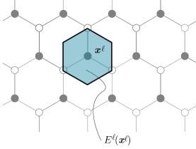
Figure 7: The hexagon $E^{\ell}(\mathbf{x}^{\ell})$.

Let ${{}\mathchoice{\mbox{\boldmath$\displaystyle\mathchar 287\relax$}}{\mbox{\boldmath$\textstyle\mathchar 287\relax$}}{\mbox{\boldmath$\scriptstyle\mathchar 287\relax$}}{\mbox{\boldmath$\scriptscriptstyle\mathchar 287\relax$}}}_{E^{\ell}(\mathbf{x}^{\ell})}(\mathbf{x})$ be the characteristic function of $E^{\ell}(\mathbf{x}^{\ell})$, i.e., it is equal to $1$ if $\mathbf{x}\in E^{\ell}(\mathbf{x}^{\ell})$ and $0$ otherwise, and let

$$W^{\mathcal{Z}}_{\ell}(\mathbf{x}):=\sum_{\mathbf{x}^{\ell}\in L_{2}(\ell)\cap\Omega} \Bigg{(}(\partial^{2}_{\mathbf{d}_{1}\mathbf{p}_{3}}w(\mathbf{x}^{\ell}))^{2}+(\partial^{2}_{\mathbf{d}_{1}\mathbf{p}_{1}}w(\mathbf{x}^{\ell}))^{2}+(\partial^{2}_{\mathbf{d}_{2}\mathbf{p}_{2}}w(\mathbf{x}^{\ell}))^{2}$$

$$+(\partial^{2}_{\mathbf{d}_{2}\mathbf{p}_{3}}w(\mathbf{x}^{\ell}))^{2}+(\partial^{2}_{\mathbf{d}_{3}\mathbf{p}_{1}}w(\mathbf{x}^{\ell}))^{2}+(\partial^{2}_{\mathbf{d}_{3}\mathbf{p}_{2}}w(\mathbf{x}^{\ell}))^{2}\Bigg{)}{{}\mathchoice{\mbox{\boldmath$\displaystyle\mathchar 287\relax$}}{\mbox{\boldmath$\textstyle\mathchar 287\relax$}}{\mbox{\boldmath$\scriptstyle\mathchar 287\relax$}}{\mbox{\boldmath$\scriptscriptstyle\mathchar 287\relax$}}}_{E^{\ell}(\mathbf{x}^{\ell})}(\mathbf{x}).$$

Then, we may simply write

$$\mathcal{U}^{\mathcal{Z}}_{\ell}=\frac{1}{2}\frac{8\sqrt{3}}{9}k^{\mathcal{Z}}\int_{\Omega}W^{\mathcal{Z}}_{\ell}(\mathbf{x})\,d\mathbf{x}+o(\ell^{2}),$$

and since $W^{\mathcal{Z}}_{\ell}$ converges, as $\ell$ goes to zero, to

$$(\partial^{2}_{\mathbf{d}_{1}\mathbf{p}_{3}}w)^{2}+(\partial^{2}_{\mathbf{d}_{1}\mathbf{p}_{1}}w)^{2}+(\partial^{2}_{\mathbf{d}_{2}\mathbf{p}_{2}}w)^{2}+(\partial^{2}_{\mathbf{d}_{2}\mathbf{p}_{3}}w)^{2}+(\partial^{2}_{\mathbf{d}_{3}\mathbf{p}_{1}}w)^{2}+(\partial^{2}_{\mathbf{d}_{3}\mathbf{p}_{2}}w)^{2},$$

we deduce that

$$\lim_{\ell\to 0}\mathcal{U}^{\mathcal{Z}}_{\ell}=\frac{1}{2}\frac{8\sqrt{3}}{9}k^{\mathcal{Z}}\int_{\Omega} (\partial^{2}_{\mathbf{d}_{1}\mathbf{p}_{3}}w)^{2}+(\partial^{2}_{\mathbf{d}_{1}\mathbf{p}_{1}}w)^{2}+(\partial^{2}_{\mathbf{d}_{2}\mathbf{p}_{2}}w)^{2}$$ (31)

$$+(\partial^{2}_{\mathbf{d}_{2}\mathbf{p}_{3}}w)^{2}+(\partial^{2}_{\mathbf{d}_{3}\mathbf{p}_{1}}w)^{2}+(\partial^{2}_{\mathbf{d}_{3}\mathbf{p}_{2}}w)^{2}\,d\mathbf{x}=:\mathcal{U}^{\mathcal{Z}}_{0}(w).$$

The functional $\mathcal{U}^{\mathcal{Z}}_{0}$, defined in (31), is the continuum limit of the Z-dihedral energy.

Working in a similar manner, we find the continuum limit of the C-dihedral energy:

$$\lim_{\ell\to 0}\mathcal{U}^{\mathcal{C}}_{\ell}=\frac{1}{2}\frac{16\sqrt{3}}{9}k^{\mathcal{C}}\int_{\Omega}\sum_{i=1}^{3}\Big{(}\partial^{2}_{\mathbf{p}_{i}\mathbf{p}_{i}^{\perp}}w\Big{)}^{2}\,d\mathbf{x}=:\mathcal{U}^{\mathcal{C}}_{0}(w),$$ (32)

and the continuum limit of the self-energy:

$$\lim_{\ell\to 0}\mathcal{U}^{(s)}_{\ell}=-\frac{4}{9}{{}\mathchoice{\mbox{\boldmath$\displaystyle\mathchar 284\relax$}}{\mbox{\boldmath$\textstyle\mathchar 284\relax$}}{\mbox{\boldmath$\scriptstyle\mathchar 284\relax$}}{\mbox{\boldmath$\scriptscriptstyle\mathchar 284\relax$}}}_{0}\int_{\Omega}(\partial^{2}_{\mathbf{p}_{1}\mathbf{p}_{1}}w+\partial^{2}_{\mathbf{p}_{2}\mathbf{p}_{2}}w+\partial^{2}_{\mathbf{p}_{1}\mathbf{p}_{2}}w\Big{)}^{2}\,d\mathbf{x}=:\mathcal{U}^{(s)}_{0}(w).$$ (33)

Detailed calculations leading to (32) and (33) are found in Appendix A.3.

The total bending limit energy is therefore

$$\mathcal{U}^{(b)}_{0}(w):=\mathcal{U}^{\mathcal{Z}}_{0}(w)+\mathcal{U}^{\mathcal{C}}_{0}(w)+\mathcal{U}^{(s)}_{0}(w).$$ (34)

6 The equivalent plate equation

In this section we rewrite the limit energies in a more amenable form. We start by manipulating the limit C-dihedral energy. We first note that

$$\partial^{2}_{\mathbf{p}_{2}\mathbf{p}_{2}^{\perp}}w =\nabla^{2}w\mathbf{p}_{2}\cdot\mathbf{p}_{2}^{\perp}=\nabla^{2}w(-\frac{1}{2}\mathbf{p}_{1}+\frac{\sqrt{3}}{2}\mathbf{p}_{1}^{\perp})\cdot(-\frac{\sqrt{3}}{2}\mathbf{p}_{1}-\frac{1}{2}\mathbf{p}_{1}^{\perp})$$

$$=\frac{\sqrt{3}}{4}\partial^{2}_{\mathbf{p}_{1}\mathbf{p}_{1}}w-\frac{\sqrt{3}}{4}\partial^{2}_{\mathbf{p}_{1}^{\perp}\mathbf{p}_{1}^{\perp}}w-\frac{1}{2}\partial^{2}_{\mathbf{p}_{1}\mathbf{p}_{1}^{\perp}}w,$$ (35)

and similarly

$$\partial^{2}_{\mathbf{p}_{3}\mathbf{p}_{3}^{\perp}}w=-\frac{\sqrt{3}}{4}\partial^{2}_{\mathbf{p}_{1}\mathbf{p}_{1}}w+\frac{\sqrt{3}}{4}\partial^{2}_{\mathbf{p}_{1}^{\perp}\mathbf{p}_{1}^{\perp}}w-\frac{1}{2}\partial^{2}_{\mathbf{p}_{1}\mathbf{p}_{1}^{\perp}}w,$$

from which we find that

$$\sum_{i=1}^{3}\Big{(}\partial^{2}_{\mathbf{p}_{i}\mathbf{p}_{i}^{\perp}}w\Big{)}^{2} =(\partial^{2}_{\mathbf{p}_{1}\mathbf{p}_{1}^{\perp}}w)^{2}+\Big{(}\frac{\sqrt{3}}{4}\partial^{2}_{\mathbf{p}_{1}\mathbf{p}_{1}}w-\frac{\sqrt{3}}{4}\partial^{2}_{\mathbf{p}_{1}^{\perp}\mathbf{p}_{1}^{\perp}}w-\frac{1}{2}\partial^{2}_{\mathbf{p}_{1}\mathbf{p}_{1}^{\perp}}w\Big{)}^{2}$$

$$\quad+\Big{(}-\frac{\sqrt{3}}{4}\partial^{2}_{\mathbf{p}_{1}\mathbf{p}_{1}}w+\frac{\sqrt{3}}{4}\partial^{2}_{\mathbf{p}_{1}^{\perp}\mathbf{p}_{1}^{\perp}}w-\frac{1}{2}\partial^{2}_{\mathbf{p}_{1}\mathbf{p}_{1}^{\perp}}w)^{2}$$

$$=\frac{3}{2}(\partial^{2}_{\mathbf{p}_{1}\mathbf{p}_{1}^{\perp}}w)^{2}+\frac{3}{8}\Big{(}\partial^{2}_{\mathbf{p}_{1}\mathbf{p}_{1}}w-\partial^{2}_{\mathbf{p}_{1}^{\perp}\mathbf{p}_{1}^{\perp}}w\Big{)}^{2}$$

$$=\frac{3}{2}(\partial^{2}_{\mathbf{p}_{1}\mathbf{p}_{1}^{\perp}}w)^{2}+\frac{3}{8}\Big{(}\partial^{2}_{\mathbf{p}_{1}\mathbf{p}_{1}}w+\partial^{2}_{\mathbf{p}_{1}^{\perp}\mathbf{p}_{1}^{\perp}}w\Big{)}^{2}-\frac{3}{2}\partial^{2}_{\mathbf{p}_{1}\mathbf{p}_{1}}w\partial^{2}_{\mathbf{p}_{1}^{\perp}\mathbf{p}_{1}^{\perp}}w$$

$$=\frac{3}{8}(\Delta w)^{2}-\frac{3}{2}\det\nabla^{2}w,$$ (36)

where $\Delta w$ denotes the Laplacian of $w$. Hence, the C-dihedral energy defined in (32) rewrites as

$$\mathcal{U}^{\mathcal{C}}_{0}(w) =\frac{1}{2}\frac{16\sqrt{3}}{9}k^{\mathcal{C}}\int_{\Omega}\sum_{i=1}^{3}\Big{(}\partial^{2}_{\mathbf{p}_{i}\mathbf{p}_{i}^{\perp}}w\Big{)}^{2}\,d\mathbf{x}=\frac{1}{2}\frac{2\sqrt{3}}{3}k^{\mathcal{C}}\int_{\Omega}(\Delta w)^{2}-4\det\nabla^{2}w\,d\mathbf{x}.$$ (37)

We now tackle the Z-dihedral energy. Recalling (31), by a calculation similar to that carried on in (35) we find

$$\partial^{2}_{\mathbf{d}_{1}\mathbf{p}_{3}}w=-\frac{\sqrt{3}}{2}\partial^{2}_{\mathbf{d}_{1}\mathbf{d}_{1}}w-\frac{1}{2}\partial^{2}_{\mathbf{d}_{1}\mathbf{d}_{1}^{\perp}}w\quad\mbox{and}\quad\partial^{2}_{\mathbf{d}_{1}\mathbf{p}_{1}}w=+\frac{\sqrt{3}}{2}\partial^{2}_{\mathbf{d}_{1}\mathbf{d}_{1}}w-\frac{1}{2}\partial^{2}_{\mathbf{d}_{1}\mathbf{d}_{1}^{\perp}}w,$$

where $\mathbf{d}_{i}^{\perp}=\mathbf{e}_{3}\times\mathbf{d}_{i}$, and from these equations we deduce that

$$(\partial^{2}_{\mathbf{d}_{1}\mathbf{p}_{1}}w)^{2}+(\partial^{2}_{\mathbf{d}_{1}\mathbf{p}_{3}}w)^{2}=\frac{3}{2}(\partial^{2}_{\mathbf{d}_{1}\mathbf{d}_{1}}w)^{2}+\frac{1}{2}(\partial^{2}_{\mathbf{d}_{1}\mathbf{d}_{1}^{\perp}}w)^{2}.$$

Similar identities hold for $\mathbf{d}_{2}$ and $\mathbf{d}_{3}$. Thence, we find that the Z-dihedral energy takes the form

$$\mathcal{U}^{\mathcal{Z}}_{0}(w) =\frac{1}{2}\frac{8\sqrt{3}}{9}k^{\mathcal{Z}}\int_{\Omega}(\partial^{2}_{\mathbf{d}_{1}\mathbf{p}_{3}}w)^{2}+(\partial^{2}_{\mathbf{d}_{1}\mathbf{p}_{1}}w)^{2}+(\partial^{2}_{\mathbf{d}_{2}\mathbf{p}_{2}}w)^{2}$$

$$\hskip 85.35826pt+(\partial^{2}_{\mathbf{d}_{2}\mathbf{p}_{3}}w)^{2}+(\partial^{2}_{\mathbf{d}_{3}\mathbf{p}_{1}}w)^{2}+(\partial^{2}_{\mathbf{d}_{3}\mathbf{p}_{2}}w)^{2}\,d\mathbf{x}$$

$$=\frac{1}{2}\frac{8\sqrt{3}}{9}k^{\mathcal{Z}}\int_{\Omega}\frac{3}{2}\sum_{i=1}^{3}(\partial^{2}_{\mathbf{d}_{i}\mathbf{d}_{i}}w)^{2}+\frac{1}{2}\sum_{i=1}^{3}(\partial^{2}_{\mathbf{d}_{i}\mathbf{d}_{i}^{\perp}}w)^{2}\,d\mathbf{x}.$$

The second sum is equal, as it can be checked, to the last line of (36), and with a similar calculation we also find that

$$\sum_{i=1}^{3}(\partial^{2}_{\mathbf{d}_{i}\mathbf{d}_{i}}w)^{2}=\frac{9}{8}(\Delta w)^{2}-\frac{3}{2}\det\nabla^{2}w,$$

and hence

$$\mathcal{U}^{\mathcal{Z}}_{0}(w) =\frac{1}{2}\frac{8\sqrt{3}}{9}k^{\mathcal{Z}}\int_{\Omega}\frac{3}{2}\Bigg{(}\frac{9}{8}(\Delta w)^{2}-\frac{3}{2}\det\nabla^{2}w\Bigg{)}+\frac{1}{2}\Bigg{(}\frac{3}{8}(\Delta w)^{2}-\frac{3}{2}\det\nabla^{2}w\Bigg{)}\,d\mathbf{x}$$

$$=\frac{1}{2}\frac{8\sqrt{3}}{9}k^{\mathcal{Z}}\int_{\Omega}\frac{15}{8}(\Delta w)^{2}-3\det\nabla^{2}w\,d\mathbf{x}$$

$$=\frac{1}{2}\frac{5\sqrt{3}}{3}k^{\mathcal{Z}}\int_{\Omega}(\Delta w)^{2}-\frac{8}{5}\det\nabla^{2}w\,d\mathbf{x}.$$ (38)

We now deal with the self-energy. Again with a calculation similar to that carried on in (35) we find

$$\partial^{2}_{\mathbf{p}_{1}\mathbf{p}_{2}}w =-\frac{1}{2}\partial^{2}_{\mathbf{p}_{1}\mathbf{p}_{1}}w+\frac{\sqrt{3}}{2}\partial^{2}_{\mathbf{p}_{1}\mathbf{p}_{1}^{\perp}}w$$

$$\partial^{2}_{\mathbf{p}_{2}\mathbf{p}_{2}}w =\frac{1}{4}\partial^{2}_{\mathbf{p}_{1}\mathbf{p}_{1}}w+\frac{{3}}{4}\partial^{2}_{\mathbf{p}_{1}^{\perp}\mathbf{p}_{1}^{\perp}}w-\frac{\sqrt{3}}{2}\partial^{2}_{\mathbf{p}_{1}\mathbf{p}_{1}^{\perp}}w,$$

and hence

$$\mathcal{U}^{(s)}_{0}(w) =-\frac{4}{9}{{}\mathchoice{\mbox{\boldmath$\displaystyle\mathchar 284\relax$}}{\mbox{\boldmath$\textstyle\mathchar 284\relax$}}{\mbox{\boldmath$\scriptstyle\mathchar 284\relax$}}{\mbox{\boldmath$\scriptscriptstyle\mathchar 284\relax$}}}_{0}\int_{\Omega}(\partial^{2}_{\mathbf{p}_{1}\mathbf{p}_{1}}w+\partial^{2}_{\mathbf{p}_{2}\mathbf{p}_{2}}w+\partial^{2}_{\mathbf{p}_{1}\mathbf{p}_{2}}w\Big{)}^{2}\,d\mathbf{x}$$

$$=-\frac{4}{9}{{}\mathchoice{\mbox{\boldmath$\displaystyle\mathchar 284\relax$}}{\mbox{\boldmath$\textstyle\mathchar 284\relax$}}{\mbox{\boldmath$\scriptstyle\mathchar 284\relax$}}{\mbox{\boldmath$\scriptscriptstyle\mathchar 284\relax$}}}_{0}\int_{\Omega}(\frac{3}{4}\partial^{2}_{\mathbf{p}_{1}\mathbf{p}_{1}}w+\frac{3}{4}\partial^{2}_{\mathbf{p}_{1}^{\perp}\mathbf{p}_{1}^{\perp}}w\Big{)}^{2}\,d\mathbf{x}$$

$$=-\frac{1}{2}\frac{{{}\mathchoice{\mbox{\boldmath$\displaystyle\mathchar 284\relax$}}{\mbox{\boldmath$\textstyle\mathchar 284\relax$}}{\mbox{\boldmath$\scriptstyle\mathchar 284\relax$}}{\mbox{\boldmath$\scriptscriptstyle\mathchar 284\relax$}}}_{0}}{2}\int_{\Omega}(\Delta w)^{2}\,d\mathbf{x}.$$ (39)

By summing (37), (38), and (39), we find the total bending energy, defined in (34):

$$\mathcal{U}^{(b)}_{0}(w)= \frac{1}{2}\int_{\Omega}\Bigg{(}\frac{5\sqrt{3}}{3}k^{\mathcal{Z}}+\frac{2\sqrt{3}}{3}k^{\mathcal{C}}-\frac{{{}\mathchoice{\mbox{\boldmath$\displaystyle\mathchar 284\relax$}}{\mbox{\boldmath$\textstyle\mathchar 284\relax$}}{\mbox{\boldmath$\scriptstyle\mathchar 284\relax$}}{\mbox{\boldmath$\scriptscriptstyle\mathchar 284\relax$}}}_{0}}{2}\Bigg{)}(\Delta w)^{2}$$

$$\hskip 85.35826pt+\Bigg{(}-\frac{8}{5}\frac{5\sqrt{3}}{3}k^{\mathcal{Z}}-4\frac{2\sqrt{3}}{3}k^{\mathcal{C}}\Bigg{)}\det\nabla^{2}w\,d\mathbf{x},$$ (40)

$$=\frac{1}{2}\int_{\Omega}\mathcal{D}(\Delta w)^{2}+\mathcal{D}_{G}\det\nabla^{2}w\,d\mathbf{x},$$ (41)

where

$$\mathcal{D}:=\frac{5\sqrt{3}}{3}k^{\mathcal{Z}}+\frac{2\sqrt{3}}{3}k^{\mathcal{C}}-\frac{{{}\mathchoice{\mbox{\boldmath$\displaystyle\mathchar 284\relax$}}{\mbox{\boldmath$\textstyle\mathchar 284\relax$}}{\mbox{\boldmath$\scriptstyle\mathchar 284\relax$}}{\mbox{\boldmath$\scriptscriptstyle\mathchar 284\relax$}}}_{0}}{2},\qquad\mathcal{D}_{G}:=-\frac{8}{5}\frac{5\sqrt{3}}{3}k^{\mathcal{Z}}-4\frac{2\sqrt{3}}{3}k^{\mathcal{C}}.$$ (42)

are the bending and the Gaussian stiffnesses, respectively. $\mathcal{D}_{G}$ is called Gaussian because it multiplies the Gaussian curvature $\det\nabla^{2}w$, while $\Delta w$ is twice the mean curvature. The analytical expression for the bending stiffness (42)₁ coincides with the one deduced in [28, 15], within a discrete mechanical framework, if one assumes that $k^{\mathcal{Z}}\equiv k^{\mathcal{C}}$. It clearly shows that the origin of the bending stiffness is twofold: a part depends on the dihedral contribution, and a part on the self-stress. Quite surprisingly, the self-stress has no role in the Gaussian stiffness. It is worth noticing that in the above approach there is no need of introducing any questionable effective thickness parameter.

7 Numerical results

In this section, we adopt the 2nd-generation Brenner potential [6] to obtain quantitative results for the continuum material parameters deduced in Sec. 6.

The 2nd-generation REBO potentials developed for hydrocarbons by Brenner et al. in [6] accommodate up to third-nearest-neighbor interactions through a bond-order function depending, in particular, on dihedral angles. Following Appendix B of [14], we here give a short account of the form of this potential.

The binding energy $V$ of an atomic aggregate is given as a sum over nearest neighbors:

$$V=\sum_{i}\sum_{j<i}V_{ij}\,;$$ (43)

the interatomic potential $V_{ij}$ is given by

$$V_{ij}=V_{R}(r_{ij})+b_{ij}V_{A}(r_{ij}),$$ (44)

where the individual effects of the repulsion and attraction functions $V_{R}(r_{ij})$ and $V_{A}(r_{ij})$, which model pair-wise interactions of atoms $i$ and $j$ depending on their distance $r_{ij}$, are modulated by the bond-order function $b_{ij}$. The repulsion and attraction functions have the following forms:

$$V_{A}(r) =-f^{C}(r)\sum_{n=1}^{3}B_{n}e^{-{{}\mathchoice{\mbox{\boldmath$\displaystyle\mathchar 268\relax$}}{\mbox{\boldmath$\textstyle\mathchar 268\relax$}}{\mbox{\boldmath$\scriptstyle\mathchar 268\relax$}}{\mbox{\boldmath$\scriptscriptstyle\mathchar 268\relax$}}}_{n}r}\,,$$ (45)

$$V_{R}(r) =f^{C}(r)\left(1+\frac{Q}{r}\right)Ae^{-{{}\mathchoice{\mbox{\boldmath$\displaystyle\mathchar 267\relax$}}{\mbox{\boldmath$\textstyle\mathchar 267\relax$}}{\mbox{\boldmath$\scriptstyle\mathchar 267\relax$}}{\mbox{\boldmath$\scriptscriptstyle\mathchar 267\relax$}}}r}\,,$$

where $f^{C}(r)$ is a cutoff function limiting the range of covalent interactions, and where $Q$, $A$, $B_{n}$, $\textstyle\mathchar 267\relax$, and $\textstyle\mathchar 268\relax$, are parameters to be chosen fit to some material-specific dataset. The remaining ingredient in (44) is the bond-order function:

$$b_{ij}=\frac{1}{2}(b_{ij}^{{{}\mathchoice{\mbox{\boldmath$\displaystyle\mathchar 283\relax$}}{\mbox{\boldmath$\textstyle\mathchar 283\relax$}}{\mbox{\boldmath$\scriptstyle\mathchar 283\relax$}}{\mbox{\boldmath$\scriptscriptstyle\mathchar 283\relax$}}}-{{}\mathchoice{\mbox{\boldmath$\displaystyle\mathchar 281\relax$}}{\mbox{\boldmath$\textstyle\mathchar 281\relax$}}{\mbox{\boldmath$\scriptstyle\mathchar 281\relax$}}{\mbox{\boldmath$\scriptscriptstyle\mathchar 281\relax$}}}}+b_{ji}^{{{}\mathchoice{\mbox{\boldmath$\displaystyle\mathchar 283\relax$}}{\mbox{\boldmath$\textstyle\mathchar 283\relax$}}{\mbox{\boldmath$\scriptstyle\mathchar 283\relax$}}{\mbox{\boldmath$\scriptscriptstyle\mathchar 283\relax$}}}-{{}\mathchoice{\mbox{\boldmath$\displaystyle\mathchar 281\relax$}}{\mbox{\boldmath$\textstyle\mathchar 281\relax$}}{\mbox{\boldmath$\scriptstyle\mathchar 281\relax$}}{\mbox{\boldmath$\scriptscriptstyle\mathchar 281\relax$}}}})+b_{ij}^{{}\mathchoice{\mbox{\boldmath$\displaystyle\mathchar 281\relax$}}{\mbox{\boldmath$\textstyle\mathchar 281\relax$}}{\mbox{\boldmath$\scriptstyle\mathchar 281\relax$}}{\mbox{\boldmath$\scriptscriptstyle\mathchar 281\relax$}}}\,,$$ (46)

where apexes $\textstyle\mathchar 283\relax$ and $\textstyle\mathchar 281\relax$ refer to two types of bonds: the strong covalent $\textstyle\mathchar 283\relax$-bonds between atoms in one and the same given plane, and the $\textstyle\mathchar 281\relax$-bonds responsible for interlayer interactions, which are perpendicular to the plane of $\textstyle\mathchar 283\relax$-bonds. The role of function $b_{ij}^{{{}\mathchoice{\mbox{\boldmath$\displaystyle\mathchar 283\relax$}}{\mbox{\boldmath$\textstyle\mathchar 283\relax$}}{\mbox{\boldmath$\scriptstyle\mathchar 283\relax$}}{\mbox{\boldmath$\scriptscriptstyle\mathchar 283\relax$}}}-{{}\mathchoice{\mbox{\boldmath$\displaystyle\mathchar 281\relax$}}{\mbox{\boldmath$\textstyle\mathchar 281\relax$}}{\mbox{\boldmath$\scriptstyle\mathchar 281\relax$}}{\mbox{\boldmath$\scriptscriptstyle\mathchar 281\relax$}}}}$ is to account for the local coordination of, and the bond angles relative to, atoms $i$ and $j$; its form is:

$$b_{ij}^{{{}\mathchoice{\mbox{\boldmath$\displaystyle\mathchar 283\relax$}}{\mbox{\boldmath$\textstyle\mathchar 283\relax$}}{\mbox{\boldmath$\scriptstyle\mathchar 283\relax$}}{\mbox{\boldmath$\scriptscriptstyle\mathchar 283\relax$}}}-{{}\mathchoice{\mbox{\boldmath$\displaystyle\mathchar 281\relax$}}{\mbox{\boldmath$\textstyle\mathchar 281\relax$}}{\mbox{\boldmath$\scriptstyle\mathchar 281\relax$}}{\mbox{\boldmath$\scriptscriptstyle\mathchar 281\relax$}}}}=\left(1+\sum_{k\neq i,j}f_{ik}^{C}(r_{ik})G(\cos{{}\mathchoice{\mbox{\boldmath$\displaystyle\mathchar 274\relax$}}{\mbox{\boldmath$\textstyle\mathchar 274\relax$}}{\mbox{\boldmath$\scriptstyle\mathchar 274\relax$}}{\mbox{\boldmath$\scriptscriptstyle\mathchar 274\relax$}}}_{ijk})\,e^{{{}\mathchoice{\mbox{\boldmath$\displaystyle\mathchar 277\relax$}}{\mbox{\boldmath$\textstyle\mathchar 277\relax$}}{\mbox{\boldmath$\scriptstyle\mathchar 277\relax$}}{\mbox{\boldmath$\scriptscriptstyle\mathchar 277\relax$}}}_{ijk}}+P_{ij}(N_{i}^{C},N_{i}^{H})\right)^{-1/2}\,.$$ (47)

Here, for each fixed pair of indices $(i,j)$, (a) the cutoff function $f_{ik}^{C}$ limits the interactions of atom $i$ to those with its nearest neighbors; (b) ${{}\mathchoice{\mbox{\boldmath$\displaystyle\mathchar 277\relax$}}{\mbox{\boldmath$\textstyle\mathchar 277\relax$}}{\mbox{\boldmath$\scriptstyle\mathchar 277\relax$}}{\mbox{\boldmath$\scriptscriptstyle\mathchar 277\relax$}}}_{ijk}$ is a string of parameters designed to prevent attraction in some specific situations; (c) function $P_{ij}$ depends on $N_{i}^{C}$ and $N_{i}^{H}$, the numbers of $C$ and $H$ atoms that are nearest neighbors of atom $i$; it is meant to adjust the bond-order function according to the environment of the C atoms in one or another molecule; (d) for solid-state carbon, the values of both the string ${{}\mathchoice{\mbox{\boldmath$\displaystyle\mathchar 277\relax$}}{\mbox{\boldmath$\textstyle\mathchar 277\relax$}}{\mbox{\boldmath$\scriptstyle\mathchar 277\relax$}}{\mbox{\boldmath$\scriptscriptstyle\mathchar 277\relax$}}}_{ijk}$ and the function $P_{ij}$ are taken null; (e) function $G$ modulates the contribution of each nearest neighbour of atom $i$ in terms of the cosine of the angle between the $ij$ and $ik$ bonds; its analytic form is given by three sixth-order polynomial splines. Function $b_{ij}^{{}\mathchoice{\mbox{\boldmath$\displaystyle\mathchar 281\relax$}}{\mbox{\boldmath$\textstyle\mathchar 281\relax$}}{\mbox{\boldmath$\scriptstyle\mathchar 281\relax$}}{\mbox{\boldmath$\scriptscriptstyle\mathchar 281\relax$}}}$ is given a split representation:

$$b_{ij}^{{}\mathchoice{\mbox{\boldmath$\displaystyle\mathchar 281\relax$}}{\mbox{\boldmath$\textstyle\mathchar 281\relax$}}{\mbox{\boldmath$\scriptstyle\mathchar 281\relax$}}{\mbox{\boldmath$\scriptscriptstyle\mathchar 281\relax$}}}=\Pi_{ij}^{RC}+b_{ij}^{DH},$$ (48)

where the first addendum $\Pi_{ij}^{RC}$ depends on whether the bond between atoms $i$ and $j$ has a radical character and on whether it is part of a conjugated system, while the second addendum $b_{ij}^{DH}$ depends on dihedral angles and has the following form:

$$b_{ij}^{DH}=T_{ij}(N_{i}^{t},N_{j}^{t},N_{ij}^{\rm conj})\left(\sum_{k(\neq i,j)}\sum_{k(\neq i,j)}\big{(}1-\cos^{2}\Theta_{ijkl}\big{)}f_{ik}^{C}(r_{ik})f_{jl}^{C}(r_{jl})\right)\,,$$ (49)

where function $T_{ij}$ is a tricubic spline depending on $N_{i}^{t}=N_{i}^{C}+N_{i}^{H}$, $N_{j}^{t}$, and $N_{ij}^{\rm conj}$, a function of local conjugation, and the dihedral angle is defined as

$$\cos\Theta_{ijkl}=\mathbf{n}_{jik}\cdot\mathbf{n}_{ijl},\quad\mathbf{n}_{jik}=\frac{\mathbf{r}_{ji}\times\mathbf{r}_{ik}}{|\mathbf{r}_{ji}\times\mathbf{r}_{ik}|},\;\mathbf{n}_{jil}=\frac{\mathbf{r}_{ij}\times\mathbf{r}_{il}}{|\mathbf{r}_{ij}\times\mathbf{r}_{jl}|}.$$ (50)

The values of the constant $k^{\mathcal{Z}}$ and $k^{\mathcal{C}}$ can be deduced by deriving twice of the potential, and computing the result in the ground state (GS): $r_{ij}=\ell$, ${{}\mathchoice{\mbox{\boldmath$\displaystyle\mathchar 274\relax$}}{\mbox{\boldmath$\textstyle\mathchar 274\relax$}}{\mbox{\boldmath$\scriptstyle\mathchar 274\relax$}}{\mbox{\boldmath$\scriptscriptstyle\mathchar 274\relax$}}}_{ijk}=2/3{{}\mathchoice{\mbox{\boldmath$\displaystyle\mathchar 281\relax$}}{\mbox{\boldmath$\textstyle\mathchar 281\relax$}}{\mbox{\boldmath$\scriptstyle\mathchar 281\relax$}}{\mbox{\boldmath$\scriptscriptstyle\mathchar 281\relax$}}}$, $\Theta_{ijkl}=0$. In particular, we find:

$$k^{\Theta}:=k^{\mathcal{Z}}=k^{\mathcal{C}}=\partial^{2}_{\Theta_{ijkl}}V_{ij}|_{GS}=2TV_{A}(\ell),$$ (51)

where $T$ is the value of $T_{ij}$ in the GS.

Remark 1

With this notation the bending stiffness becomes:

$$\mathcal{D}=\frac{7\sqrt{3}}{3}k^{\Theta}-\frac{{{}\mathchoice{\mbox{\boldmath$\displaystyle\mathchar 284\relax$}}{\mbox{\boldmath$\textstyle\mathchar 284\relax$}}{\mbox{\boldmath$\scriptstyle\mathchar 284\relax$}}{\mbox{\boldmath$\scriptscriptstyle\mathchar 284\relax$}}}_{0}}{2}.$$

This expression coincides with that given in [28]:

$$\mathcal{D}=\frac{V_{A}(r_{0})}{2}\left((b_{0}^{{{}\mathchoice{\mbox{\boldmath$\displaystyle\mathchar 283\relax$}}{\mbox{\boldmath$\textstyle\mathchar 283\relax$}}{\mbox{\boldmath$\scriptstyle\mathchar 283\relax$}}{\mbox{\boldmath$\scriptscriptstyle\mathchar 283\relax$}}}-{{}\mathchoice{\mbox{\boldmath$\displaystyle\mathchar 281\relax$}}{\mbox{\boldmath$\textstyle\mathchar 281\relax$}}{\mbox{\boldmath$\scriptstyle\mathchar 281\relax$}}{\mbox{\boldmath$\scriptscriptstyle\mathchar 281\relax$}}}})^{\prime}-\frac{14T_{0}}{\sqrt{3}}\right),$$

after noticing that

$$V_{A}(r_{0})(b_{0}^{{{}\mathchoice{\mbox{\boldmath$\displaystyle\mathchar 283\relax$}}{\mbox{\boldmath$\textstyle\mathchar 283\relax$}}{\mbox{\boldmath$\scriptstyle\mathchar 283\relax$}}{\mbox{\boldmath$\scriptscriptstyle\mathchar 283\relax$}}}-{{}\mathchoice{\mbox{\boldmath$\displaystyle\mathchar 281\relax$}}{\mbox{\boldmath$\textstyle\mathchar 281\relax$}}{\mbox{\boldmath$\scriptstyle\mathchar 281\relax$}}{\mbox{\boldmath$\scriptscriptstyle\mathchar 281\relax$}}}})^{\prime}\equiv-{{}\mathchoice{\mbox{\boldmath$\displaystyle\mathchar 284\relax$}}{\mbox{\boldmath$\textstyle\mathchar 284\relax$}}{\mbox{\boldmath$\scriptstyle\mathchar 284\relax$}}{\mbox{\boldmath$\scriptscriptstyle\mathchar 284\relax$}}}_{0},\quad-V_{A}(r_{0})\left(\frac{7T_{0}}{\sqrt{3}}\right)\equiv 2TV_{A}(\ell)\frac{7}{\sqrt{3}}=\frac{7}{\sqrt{3}}k^{\Theta}.$$

Instead, in references [4] and [21] the dihedral energies are not contemplated and the bending stiffness found, up to notational differences, coincides with ours after setting $k^{\Theta}=0$.

With the values reported in [6], we get:

$$k^{\Theta}=0.0282\;\textrm{nN nm}=0.1764\;\textrm{eV}.$$ (52)

From [14], we take the value of the selfstress ${{}\mathchoice{\mbox{\boldmath$\displaystyle\mathchar 284\relax$}}{\mbox{\boldmath$\textstyle\mathchar 284\relax$}}{\mbox{\boldmath$\scriptstyle\mathchar 284\relax$}}{\mbox{\boldmath$\scriptscriptstyle\mathchar 284\relax$}}}_{0}$:

$${{}\mathchoice{\mbox{\boldmath$\displaystyle\mathchar 284\relax$}}{\mbox{\boldmath$\textstyle\mathchar 284\relax$}}{\mbox{\boldmath$\scriptstyle\mathchar 284\relax$}}{\mbox{\boldmath$\scriptscriptstyle\mathchar 284\relax$}}}_{0}=-0.2209\;\textrm{nN nm}=-1.3787\;\textrm{eV}.$$ (53)

With (52) and (53), we obtain:

$$\mathcal{D}=\frac{7\sqrt{3}}{3}k^{\Theta}-\frac{{{}\mathchoice{\mbox{\boldmath$\displaystyle\mathchar 284\relax$}}{\mbox{\boldmath$\textstyle\mathchar 284\relax$}}{\mbox{\boldmath$\scriptstyle\mathchar 284\relax$}}{\mbox{\boldmath$\scriptscriptstyle\mathchar 284\relax$}}}_{0}}{2}=0.2247\;\textrm{nN nm}=1.4022\;\textrm{eV},$$ (54)

$$\mathcal{D}_{G}=-16\frac{\sqrt{3}}{3}k^{\Theta}=-0.2610\;\textrm{nN nm}=-1.6293\;\textrm{eV}.$$

The value of $\mathcal{D}$ is in complete agreement with the literature [27, 38]; from (52) and (53) it is possible to check that the contribution of the self-stress and the dihedral stiffness amounts to about $49.16$% and $50.84$% of the total, respectively. Neither analytical evaluation of $\mathcal{D}_{G}$, nor MD computations, have been proposed so far. The value we obtain is in good agreement with the value of $-1.52$ eV, reported in [38] and determined by means of DFT.

8 Conclusions

Starting form a discrete model inferred from MD, we have deduced a continuum theory describing the bending behavior of a graphene sheet. Atomic interactions have been modeled by exploiting the main features of the 2nd-generation Brenner potential and adopting a quadratic approximation of the energy. The deduced continuum limit fully describes the bending behavior of graphene. To our knowledge, it is the first time that an analytical expression of the Gaussian stiffness is given and an explanation of its origins at the atomistic scale is provided. We also derived a quantitative evaluation of the related constitutive parameters.

Appendix A Appendix

In order to compute the strain measures for small changes of configuration of the graphene foil, we write the displacements of the nodes in the form

$${\bf u}(\mathbf{x}^{\ell})={{}\mathchoice{\mbox{\boldmath$\displaystyle\mathchar 280\relax$}}{\mbox{\boldmath$\textstyle\mathchar 280\relax$}}{\mbox{\boldmath$\scriptstyle\mathchar 280\relax$}}{\mbox{\boldmath$\scriptscriptstyle\mathchar 280\relax$}}}\operatorname{\boldsymbol{\mathfrak{u}}}(\mathbf{x}^{\ell}),$$

where $\textstyle\mathchar 280\relax$ is a positive scalar measuring smallness and $\operatorname{\boldsymbol{\mathfrak{u}}}:=\frac{\bf u}{{{}\mathchoice{\mbox{\boldmath$\displaystyle\mathchar 280\relax$}}{\mbox{\boldmath$\textstyle\mathchar 280\relax$}}{\mbox{\boldmath$\scriptstyle\mathchar 280\relax$}}{\mbox{\boldmath$\scriptscriptstyle\mathchar 280\relax$}}}}$ stands for the displacement distribution normalized accordingly.

A.1 Change of the bond angle

Let us define the bond angle as

$$\cos({{}\mathchoice{\mbox{\boldmath$\displaystyle\mathchar 291\relax$}}{\mbox{\boldmath$\textstyle\mathchar 291\relax$}}{\mbox{\boldmath$\scriptstyle\mathchar 291\relax$}}{\mbox{\boldmath$\scriptscriptstyle\mathchar 291\relax$}}}_{i}({{}\mathchoice{\mbox{\boldmath$\displaystyle\mathchar 280\relax$}}{\mbox{\boldmath$\textstyle\mathchar 280\relax$}}{\mbox{\boldmath$\scriptstyle\mathchar 280\relax$}}{\mbox{\boldmath$\scriptscriptstyle\mathchar 280\relax$}}}))=\left(\frac{\mathbf{m}({{}\mathchoice{\mbox{\boldmath$\displaystyle\mathchar 280\relax$}}{\mbox{\boldmath$\textstyle\mathchar 280\relax$}}{\mbox{\boldmath$\scriptstyle\mathchar 280\relax$}}{\mbox{\boldmath$\scriptscriptstyle\mathchar 280\relax$}}})\cdot\mathbf{n}({{}\mathchoice{\mbox{\boldmath$\displaystyle\mathchar 280\relax$}}{\mbox{\boldmath$\textstyle\mathchar 280\relax$}}{\mbox{\boldmath$\scriptstyle\mathchar 280\relax$}}{\mbox{\boldmath$\scriptscriptstyle\mathchar 280\relax$}}})}{|\mathbf{m}({{}\mathchoice{\mbox{\boldmath$\displaystyle\mathchar 280\relax$}}{\mbox{\boldmath$\textstyle\mathchar 280\relax$}}{\mbox{\boldmath$\scriptstyle\mathchar 280\relax$}}{\mbox{\boldmath$\scriptscriptstyle\mathchar 280\relax$}}})||\mathbf{n}({{}\mathchoice{\mbox{\boldmath$\displaystyle\mathchar 280\relax$}}{\mbox{\boldmath$\textstyle\mathchar 280\relax$}}{\mbox{\boldmath$\scriptstyle\mathchar 280\relax$}}{\mbox{\boldmath$\scriptscriptstyle\mathchar 280\relax$}}})|}\right),$$ (55)

with

$$\mathbf{m}({{}\mathchoice{\mbox{\boldmath$\displaystyle\mathchar 280\relax$}}{\mbox{\boldmath$\textstyle\mathchar 280\relax$}}{\mbox{\boldmath$\scriptstyle\mathchar 280\relax$}}{\mbox{\boldmath$\scriptscriptstyle\mathchar 280\relax$}}}):=\ell\mathbf{p}_{i+1}+{{}\mathchoice{\mbox{\boldmath$\displaystyle\mathchar 280\relax$}}{\mbox{\boldmath$\textstyle\mathchar 280\relax$}}{\mbox{\boldmath$\scriptstyle\mathchar 280\relax$}}{\mbox{\boldmath$\scriptscriptstyle\mathchar 280\relax$}}}(\operatorname{\boldsymbol{\mathfrak{u}}}_{i+1}-\operatorname{\boldsymbol{\mathfrak{u}}}_{0})\quad\mbox{and}\quad\mathbf{n}({{}\mathchoice{\mbox{\boldmath$\displaystyle\mathchar 280\relax$}}{\mbox{\boldmath$\textstyle\mathchar 280\relax$}}{\mbox{\boldmath$\scriptstyle\mathchar 280\relax$}}{\mbox{\boldmath$\scriptscriptstyle\mathchar 280\relax$}}}):=\ell\mathbf{p}_{i+2}+{{}\mathchoice{\mbox{\boldmath$\displaystyle\mathchar 280\relax$}}{\mbox{\boldmath$\textstyle\mathchar 280\relax$}}{\mbox{\boldmath$\scriptstyle\mathchar 280\relax$}}{\mbox{\boldmath$\scriptscriptstyle\mathchar 280\relax$}}}(\operatorname{\boldsymbol{\mathfrak{u}}}_{i+2}-\operatorname{\boldsymbol{\mathfrak{u}}}_{0}),$$

where we have set

$$\operatorname{\boldsymbol{\mathfrak{u}}}_{0}:=\operatorname{\boldsymbol{\mathfrak{u}}}(\mathbf{x}^{\ell}),\quad\operatorname{\boldsymbol{\mathfrak{u}}}_{i}:=\operatorname{\boldsymbol{\mathfrak{u}}}(\mathbf{x}^{\ell}+\ell\mathbf{p}_{i}).$$ (56)

Then, from Taylor’s expansion we get

$${{}\mathchoice{\mbox{\boldmath$\displaystyle\mathchar 291\relax$}}{\mbox{\boldmath$\textstyle\mathchar 291\relax$}}{\mbox{\boldmath$\scriptstyle\mathchar 291\relax$}}{\mbox{\boldmath$\scriptscriptstyle\mathchar 291\relax$}}}_{i}({{}\mathchoice{\mbox{\boldmath$\displaystyle\mathchar 280\relax$}}{\mbox{\boldmath$\textstyle\mathchar 280\relax$}}{\mbox{\boldmath$\scriptstyle\mathchar 280\relax$}}{\mbox{\boldmath$\scriptscriptstyle\mathchar 280\relax$}}})={{}\mathchoice{\mbox{\boldmath$\displaystyle\mathchar 291\relax$}}{\mbox{\boldmath$\textstyle\mathchar 291\relax$}}{\mbox{\boldmath$\scriptstyle\mathchar 291\relax$}}{\mbox{\boldmath$\scriptscriptstyle\mathchar 291\relax$}}}_{i}(0)+{{}\mathchoice{\mbox{\boldmath$\displaystyle\mathchar 291\relax$}}{\mbox{\boldmath$\textstyle\mathchar 291\relax$}}{\mbox{\boldmath$\scriptstyle\mathchar 291\relax$}}{\mbox{\boldmath$\scriptscriptstyle\mathchar 291\relax$}}}_{i}^{\prime}(0)\,{{}\mathchoice{\mbox{\boldmath$\displaystyle\mathchar 280\relax$}}{\mbox{\boldmath$\textstyle\mathchar 280\relax$}}{\mbox{\boldmath$\scriptstyle\mathchar 280\relax$}}{\mbox{\boldmath$\scriptscriptstyle\mathchar 280\relax$}}}+\frac{1}{2}\,{{}\mathchoice{\mbox{\boldmath$\displaystyle\mathchar 291\relax$}}{\mbox{\boldmath$\textstyle\mathchar 291\relax$}}{\mbox{\boldmath$\scriptstyle\mathchar 291\relax$}}{\mbox{\boldmath$\scriptscriptstyle\mathchar 291\relax$}}}_{i}^{\prime\prime}(0){{}\mathchoice{\mbox{\boldmath$\displaystyle\mathchar 280\relax$}}{\mbox{\boldmath$\textstyle\mathchar 280\relax$}}{\mbox{\boldmath$\scriptstyle\mathchar 280\relax$}}{\mbox{\boldmath$\scriptscriptstyle\mathchar 280\relax$}}}^{2}+O({{}\mathchoice{\mbox{\boldmath$\displaystyle\mathchar 280\relax$}}{\mbox{\boldmath$\textstyle\mathchar 280\relax$}}{\mbox{\boldmath$\scriptstyle\mathchar 280\relax$}}{\mbox{\boldmath$\scriptscriptstyle\mathchar 280\relax$}}}^{3}),$$ (57)

where the various terms can be calculated by successive differentiations of Eq. (55). Thus,

$$-\sin({{}\mathchoice{\mbox{\boldmath$\displaystyle\mathchar 291\relax$}}{\mbox{\boldmath$\textstyle\mathchar 291\relax$}}{\mbox{\boldmath$\scriptstyle\mathchar 291\relax$}}{\mbox{\boldmath$\scriptscriptstyle\mathchar 291\relax$}}}_{i}(0)) {{}\mathchoice{\mbox{\boldmath$\displaystyle\mathchar 291\relax$}}{\mbox{\boldmath$\textstyle\mathchar 291\relax$}}{\mbox{\boldmath$\scriptstyle\mathchar 291\relax$}}{\mbox{\boldmath$\scriptscriptstyle\mathchar 291\relax$}}}_{i}^{\prime}(0)=\left.\left(\frac{\mathbf{m}({{}\mathchoice{\mbox{\boldmath$\displaystyle\mathchar 280\relax$}}{\mbox{\boldmath$\textstyle\mathchar 280\relax$}}{\mbox{\boldmath$\scriptstyle\mathchar 280\relax$}}{\mbox{\boldmath$\scriptscriptstyle\mathchar 280\relax$}}})\cdot\mathbf{n}({{}\mathchoice{\mbox{\boldmath$\displaystyle\mathchar 280\relax$}}{\mbox{\boldmath$\textstyle\mathchar 280\relax$}}{\mbox{\boldmath$\scriptstyle\mathchar 280\relax$}}{\mbox{\boldmath$\scriptscriptstyle\mathchar 280\relax$}}})}{|\mathbf{m}({{}\mathchoice{\mbox{\boldmath$\displaystyle\mathchar 280\relax$}}{\mbox{\boldmath$\textstyle\mathchar 280\relax$}}{\mbox{\boldmath$\scriptstyle\mathchar 280\relax$}}{\mbox{\boldmath$\scriptscriptstyle\mathchar 280\relax$}}})||\mathbf{n}({{}\mathchoice{\mbox{\boldmath$\displaystyle\mathchar 280\relax$}}{\mbox{\boldmath$\textstyle\mathchar 280\relax$}}{\mbox{\boldmath$\scriptstyle\mathchar 280\relax$}}{\mbox{\boldmath$\scriptscriptstyle\mathchar 280\relax$}}})|}\right)^{\prime}\right|_{{{}\mathchoice{\mbox{\boldmath$\displaystyle\mathchar 280\relax$}}{\mbox{\boldmath$\textstyle\mathchar 280\relax$}}{\mbox{\boldmath$\scriptstyle\mathchar 280\relax$}}{\mbox{\boldmath$\scriptscriptstyle\mathchar 280\relax$}}}=0}$$ (58)

$$=\frac{\mathbf{m}^{\prime}({{}\mathchoice{\mbox{\boldmath$\displaystyle\mathchar 280\relax$}}{\mbox{\boldmath$\textstyle\mathchar 280\relax$}}{\mbox{\boldmath$\scriptstyle\mathchar 280\relax$}}{\mbox{\boldmath$\scriptscriptstyle\mathchar 280\relax$}}})\cdot\mathbf{n}({{}\mathchoice{\mbox{\boldmath$\displaystyle\mathchar 280\relax$}}{\mbox{\boldmath$\textstyle\mathchar 280\relax$}}{\mbox{\boldmath$\scriptstyle\mathchar 280\relax$}}{\mbox{\boldmath$\scriptscriptstyle\mathchar 280\relax$}}})+\mathbf{m}({{}\mathchoice{\mbox{\boldmath$\displaystyle\mathchar 280\relax$}}{\mbox{\boldmath$\textstyle\mathchar 280\relax$}}{\mbox{\boldmath$\scriptstyle\mathchar 280\relax$}}{\mbox{\boldmath$\scriptscriptstyle\mathchar 280\relax$}}})\cdot\mathbf{n}^{\prime}({{}\mathchoice{\mbox{\boldmath$\displaystyle\mathchar 280\relax$}}{\mbox{\boldmath$\textstyle\mathchar 280\relax$}}{\mbox{\boldmath$\scriptstyle\mathchar 280\relax$}}{\mbox{\boldmath$\scriptscriptstyle\mathchar 280\relax$}}})}{|\mathbf{m}({{}\mathchoice{\mbox{\boldmath$\displaystyle\mathchar 280\relax$}}{\mbox{\boldmath$\textstyle\mathchar 280\relax$}}{\mbox{\boldmath$\scriptstyle\mathchar 280\relax$}}{\mbox{\boldmath$\scriptscriptstyle\mathchar 280\relax$}}})||\mathbf{n}({{}\mathchoice{\mbox{\boldmath$\displaystyle\mathchar 280\relax$}}{\mbox{\boldmath$\textstyle\mathchar 280\relax$}}{\mbox{\boldmath$\scriptstyle\mathchar 280\relax$}}{\mbox{\boldmath$\scriptscriptstyle\mathchar 280\relax$}}})|}-\frac{\mathbf{m}({{}\mathchoice{\mbox{\boldmath$\displaystyle\mathchar 280\relax$}}{\mbox{\boldmath$\textstyle\mathchar 280\relax$}}{\mbox{\boldmath$\scriptstyle\mathchar 280\relax$}}{\mbox{\boldmath$\scriptscriptstyle\mathchar 280\relax$}}})\cdot\mathbf{n}({{}\mathchoice{\mbox{\boldmath$\displaystyle\mathchar 280\relax$}}{\mbox{\boldmath$\textstyle\mathchar 280\relax$}}{\mbox{\boldmath$\scriptstyle\mathchar 280\relax$}}{\mbox{\boldmath$\scriptscriptstyle\mathchar 280\relax$}}})}{|\mathbf{m}({{}\mathchoice{\mbox{\boldmath$\displaystyle\mathchar 280\relax$}}{\mbox{\boldmath$\textstyle\mathchar 280\relax$}}{\mbox{\boldmath$\scriptstyle\mathchar 280\relax$}}{\mbox{\boldmath$\scriptscriptstyle\mathchar 280\relax$}}})||\mathbf{n}({{}\mathchoice{\mbox{\boldmath$\displaystyle\mathchar 280\relax$}}{\mbox{\boldmath$\textstyle\mathchar 280\relax$}}{\mbox{\boldmath$\scriptstyle\mathchar 280\relax$}}{\mbox{\boldmath$\scriptscriptstyle\mathchar 280\relax$}}})|}\left.\left(\frac{\mathbf{m}({{}\mathchoice{\mbox{\boldmath$\displaystyle\mathchar 280\relax$}}{\mbox{\boldmath$\textstyle\mathchar 280\relax$}}{\mbox{\boldmath$\scriptstyle\mathchar 280\relax$}}{\mbox{\boldmath$\scriptscriptstyle\mathchar 280\relax$}}})\cdot\mathbf{m}^{\prime}({{}\mathchoice{\mbox{\boldmath$\displaystyle\mathchar 280\relax$}}{\mbox{\boldmath$\textstyle\mathchar 280\relax$}}{\mbox{\boldmath$\scriptstyle\mathchar 280\relax$}}{\mbox{\boldmath$\scriptscriptstyle\mathchar 280\relax$}}})}{|\mathbf{m}({{}\mathchoice{\mbox{\boldmath$\displaystyle\mathchar 280\relax$}}{\mbox{\boldmath$\textstyle\mathchar 280\relax$}}{\mbox{\boldmath$\scriptstyle\mathchar 280\relax$}}{\mbox{\boldmath$\scriptscriptstyle\mathchar 280\relax$}}})|^{2}}+\frac{\mathbf{n}({{}\mathchoice{\mbox{\boldmath$\displaystyle\mathchar 280\relax$}}{\mbox{\boldmath$\textstyle\mathchar 280\relax$}}{\mbox{\boldmath$\scriptstyle\mathchar 280\relax$}}{\mbox{\boldmath$\scriptscriptstyle\mathchar 280\relax$}}})\cdot\mathbf{n}^{\prime}({{}\mathchoice{\mbox{\boldmath$\displaystyle\mathchar 280\relax$}}{\mbox{\boldmath$\textstyle\mathchar 280\relax$}}{\mbox{\boldmath$\scriptstyle\mathchar 280\relax$}}{\mbox{\boldmath$\scriptscriptstyle\mathchar 280\relax$}}})}{|\mathbf{n}({{}\mathchoice{\mbox{\boldmath$\displaystyle\mathchar 280\relax$}}{\mbox{\boldmath$\textstyle\mathchar 280\relax$}}{\mbox{\boldmath$\scriptstyle\mathchar 280\relax$}}{\mbox{\boldmath$\scriptscriptstyle\mathchar 280\relax$}}})|^{2}}\right)\right|_{{{}\mathchoice{\mbox{\boldmath$\displaystyle\mathchar 280\relax$}}{\mbox{\boldmath$\textstyle\mathchar 280\relax$}}{\mbox{\boldmath$\scriptstyle\mathchar 280\relax$}}{\mbox{\boldmath$\scriptscriptstyle\mathchar 280\relax$}}}=0},$$

which yields

$${{}\mathchoice{\mbox{\boldmath$\displaystyle\mathchar 291\relax$}}{\mbox{\boldmath$\textstyle\mathchar 291\relax$}}{\mbox{\boldmath$\scriptstyle\mathchar 291\relax$}}{\mbox{\boldmath$\scriptscriptstyle\mathchar 291\relax$}}}_{i}^{\prime}(0)=-\frac{\mathbf{p}_{i+2}+\frac{1}{2}\mathbf{p}_{i+1}}{|\mathbf{p}_{i+2}+\frac{1}{2}\mathbf{p}_{i+1}|}\cdot(\operatorname{\boldsymbol{\mathfrak{u}}}_{i+1}-\operatorname{\boldsymbol{\mathfrak{u}}}_{0})-\frac{\mathbf{p}_{i+1}+\frac{1}{2}\mathbf{p}_{i+2}}{|\mathbf{p}_{i+1}+\frac{1}{2}\mathbf{p}_{i+2}|}\cdot(\operatorname{\boldsymbol{\mathfrak{u}}}_{i+2}-\operatorname{\boldsymbol{\mathfrak{u}}}_{0}),$$ (59)

where we take into account that $\sin({{}\mathchoice{\mbox{\boldmath$\displaystyle\mathchar 291\relax$}}{\mbox{\boldmath$\textstyle\mathchar 291\relax$}}{\mbox{\boldmath$\scriptstyle\mathchar 291\relax$}}{\mbox{\boldmath$\scriptscriptstyle\mathchar 291\relax$}}}_{i}(0))=\frac{\sqrt{3}}{2}$, $|\mathbf{m}(0)|=|\mathbf{n}(0)|=\ell$, $|\mathbf{p}_{i+1}+\frac{1}{2}\mathbf{p}_{i+2}|=|\mathbf{p}_{i+2}+\frac{1}{2}\mathbf{p}_{i+1}|=\sqrt{3}/2$ and $\mathbf{p}_{i}\cdot\mathbf{p}_{i+1}=-1/2$.

Moreover, by differentiating Eq. (55) twice, we get

$$-\cos({{}\mathchoice{\mbox{\boldmath$\displaystyle\mathchar 291\relax$}}{\mbox{\boldmath$\textstyle\mathchar 291\relax$}}{\mbox{\boldmath$\scriptstyle\mathchar 291\relax$}}{\mbox{\boldmath$\scriptscriptstyle\mathchar 291\relax$}}}_{i}(0))\,{{}\mathchoice{\mbox{\boldmath$\displaystyle\mathchar 291\relax$}}{\mbox{\boldmath$\textstyle\mathchar 291\relax$}}{\mbox{\boldmath$\scriptstyle\mathchar 291\relax$}}{\mbox{\boldmath$\scriptscriptstyle\mathchar 291\relax$}}}^{\prime}_{i}(0)^{2}-\sin({{}\mathchoice{\mbox{\boldmath$\displaystyle\mathchar 291\relax$}}{\mbox{\boldmath$\textstyle\mathchar 291\relax$}}{\mbox{\boldmath$\scriptstyle\mathchar 291\relax$}}{\mbox{\boldmath$\scriptscriptstyle\mathchar 291\relax$}}}_{i}(0))\,{{}\mathchoice{\mbox{\boldmath$\displaystyle\mathchar 291\relax$}}{\mbox{\boldmath$\textstyle\mathchar 291\relax$}}{\mbox{\boldmath$\scriptstyle\mathchar 291\relax$}}{\mbox{\boldmath$\scriptscriptstyle\mathchar 291\relax$}}}_{i}^{\prime\prime}(0)=\left.\left(\frac{\mathbf{m}({{}\mathchoice{\mbox{\boldmath$\displaystyle\mathchar 280\relax$}}{\mbox{\boldmath$\textstyle\mathchar 280\relax$}}{\mbox{\boldmath$\scriptstyle\mathchar 280\relax$}}{\mbox{\boldmath$\scriptscriptstyle\mathchar 280\relax$}}})\cdot\mathbf{n}({{}\mathchoice{\mbox{\boldmath$\displaystyle\mathchar 280\relax$}}{\mbox{\boldmath$\textstyle\mathchar 280\relax$}}{\mbox{\boldmath$\scriptstyle\mathchar 280\relax$}}{\mbox{\boldmath$\scriptscriptstyle\mathchar 280\relax$}}})}{|\mathbf{m}({{}\mathchoice{\mbox{\boldmath$\displaystyle\mathchar 280\relax$}}{\mbox{\boldmath$\textstyle\mathchar 280\relax$}}{\mbox{\boldmath$\scriptstyle\mathchar 280\relax$}}{\mbox{\boldmath$\scriptscriptstyle\mathchar 280\relax$}}})||\mathbf{n}({{}\mathchoice{\mbox{\boldmath$\displaystyle\mathchar 280\relax$}}{\mbox{\boldmath$\textstyle\mathchar 280\relax$}}{\mbox{\boldmath$\scriptstyle\mathchar 280\relax$}}{\mbox{\boldmath$\scriptscriptstyle\mathchar 280\relax$}}})|}\right)^{\prime\prime}\right|_{{{}\mathchoice{\mbox{\boldmath$\displaystyle\mathchar 280\relax$}}{\mbox{\boldmath$\textstyle\mathchar 280\relax$}}{\mbox{\boldmath$\scriptstyle\mathchar 280\relax$}}{\mbox{\boldmath$\scriptscriptstyle\mathchar 280\relax$}}}=0},$$ (60)

which gives

$${{}\mathchoice{\mbox{\boldmath$\displaystyle\mathchar 291\relax$}}{\mbox{\boldmath$\textstyle\mathchar 291\relax$}}{\mbox{\boldmath$\scriptstyle\mathchar 291\relax$}}{\mbox{\boldmath$\scriptscriptstyle\mathchar 291\relax$}}}_{i}^{\prime\prime}(0)=-\frac{1}{\sin{{}\mathchoice{\mbox{\boldmath$\displaystyle\mathchar 291\relax$}}{\mbox{\boldmath$\textstyle\mathchar 291\relax$}}{\mbox{\boldmath$\scriptstyle\mathchar 291\relax$}}{\mbox{\boldmath$\scriptscriptstyle\mathchar 291\relax$}}}_{i}(0)}\left(\cos{{}\mathchoice{\mbox{\boldmath$\displaystyle\mathchar 291\relax$}}{\mbox{\boldmath$\textstyle\mathchar 291\relax$}}{\mbox{\boldmath$\scriptstyle\mathchar 291\relax$}}{\mbox{\boldmath$\scriptscriptstyle\mathchar 291\relax$}}}_{i}(0){{}\mathchoice{\mbox{\boldmath$\displaystyle\mathchar 291\relax$}}{\mbox{\boldmath$\textstyle\mathchar 291\relax$}}{\mbox{\boldmath$\scriptstyle\mathchar 291\relax$}}{\mbox{\boldmath$\scriptscriptstyle\mathchar 291\relax$}}}^{\prime}_{i}(0)^{2}+\left.\left(\frac{\mathbf{m}({{}\mathchoice{\mbox{\boldmath$\displaystyle\mathchar 280\relax$}}{\mbox{\boldmath$\textstyle\mathchar 280\relax$}}{\mbox{\boldmath$\scriptstyle\mathchar 280\relax$}}{\mbox{\boldmath$\scriptscriptstyle\mathchar 280\relax$}}})\cdot\mathbf{n}({{}\mathchoice{\mbox{\boldmath$\displaystyle\mathchar 280\relax$}}{\mbox{\boldmath$\textstyle\mathchar 280\relax$}}{\mbox{\boldmath$\scriptstyle\mathchar 280\relax$}}{\mbox{\boldmath$\scriptscriptstyle\mathchar 280\relax$}}})}{|\mathbf{m}({{}\mathchoice{\mbox{\boldmath$\displaystyle\mathchar 280\relax$}}{\mbox{\boldmath$\textstyle\mathchar 280\relax$}}{\mbox{\boldmath$\scriptstyle\mathchar 280\relax$}}{\mbox{\boldmath$\scriptscriptstyle\mathchar 280\relax$}}})||\mathbf{n}({{}\mathchoice{\mbox{\boldmath$\displaystyle\mathchar 280\relax$}}{\mbox{\boldmath$\textstyle\mathchar 280\relax$}}{\mbox{\boldmath$\scriptstyle\mathchar 280\relax$}}{\mbox{\boldmath$\scriptscriptstyle\mathchar 280\relax$}}})|}\right)^{\prime\prime}\right|_{{{}\mathchoice{\mbox{\boldmath$\displaystyle\mathchar 280\relax$}}{\mbox{\boldmath$\textstyle\mathchar 280\relax$}}{\mbox{\boldmath$\scriptstyle\mathchar 280\relax$}}{\mbox{\boldmath$\scriptscriptstyle\mathchar 280\relax$}}}=0}\right).$$ (61)

Computations yield that

$$\left(\frac{\mathbf{m}\cdot\mathbf{n}}{|\mathbf{m}||\mathbf{n}|}\right)^{\prime\prime} =\frac{\mathbf{m}^{\prime\prime}}{|\mathbf{m}|}\cdot\frac{\mathbf{n}}{|\mathbf{n}|}+2\,\frac{\mathbf{m}^{\prime}}{|\mathbf{m}|}\cdot\frac{\mathbf{n}^{\prime}}{|\mathbf{n}|}+\frac{\mathbf{m}}{|\mathbf{m}|}\cdot\frac{\mathbf{n}^{\prime\prime}}{|\mathbf{n}|}$$ (62)

$$-\left[\frac{\mathbf{m}^{\prime}}{|\mathbf{m}|}\cdot\frac{\mathbf{n}}{|\mathbf{n}|}+\frac{\mathbf{m}}{|\mathbf{m}|}\cdot\frac{\mathbf{n}^{\prime}}{|\mathbf{n}|}+\left(\frac{\mathbf{m}}{|\mathbf{m}|}\cdot\frac{\mathbf{n}}{|\mathbf{n}|}\right)^{\prime}\right]\left(\frac{\mathbf{m}^{\prime}}{|\mathbf{m}|}\cdot\frac{\mathbf{m}}{|\mathbf{m}|}+\frac{\mathbf{n}^{\prime}}{|\mathbf{n}|}\cdot\frac{\mathbf{n}}{|\mathbf{n}|}\right)$$

$$-\frac{\mathbf{m}}{|\mathbf{m}|}\cdot\frac{\mathbf{n}}{|\mathbf{n}|}\left[\left(\frac{|\mathbf{m}^{\prime}|}{|\mathbf{m}|}\right)^{2}+\frac{\mathbf{m}}{|\mathbf{m}|}\cdot\frac{\mathbf{m}^{\prime\prime}}{|\mathbf{m}|}-2\left(\frac{\mathbf{m}^{\prime}}{|\mathbf{m}|}\cdot\frac{\mathbf{m}}{|\mathbf{m}|}\right)^{2}\right.$$

$$\left.+\left(\frac{|\mathbf{n}^{\prime}|}{|\mathbf{n}|}\right)^{2}+\frac{\mathbf{n}}{|\mathbf{n}|}\cdot\frac{\mathbf{n}^{\prime\prime}}{|\mathbf{n}|}-2\left(\frac{\mathbf{n}^{\prime}}{|\mathbf{n}|}\cdot\frac{\mathbf{n}}{|\mathbf{n}|}\right)^{2}\right]\,.$$

Since $\mathbf{m}^{\prime\prime}(0)=\mathbf{n}^{\prime\prime}(0)=\mathbf{0}$ and $\left(\frac{\mathbf{m}\cdot\mathbf{n}}{|\mathbf{m}||\mathbf{n}|}\right)^{\prime}\Big{|}_{{{}\mathchoice{\mbox{\boldmath$\displaystyle\mathchar 280\relax$}}{\mbox{\boldmath$\textstyle\mathchar 280\relax$}}{\mbox{\boldmath$\scriptstyle\mathchar 280\relax$}}{\mbox{\boldmath$\scriptscriptstyle\mathchar 280\relax$}}}=0}=-\sin{{}\mathchoice{\mbox{\boldmath$\displaystyle\mathchar 291\relax$}}{\mbox{\boldmath$\textstyle\mathchar 291\relax$}}{\mbox{\boldmath$\scriptstyle\mathchar 291\relax$}}{\mbox{\boldmath$\scriptscriptstyle\mathchar 291\relax$}}}_{i}(0){{}\mathchoice{\mbox{\boldmath$\displaystyle\mathchar 291\relax$}}{\mbox{\boldmath$\textstyle\mathchar 291\relax$}}{\mbox{\boldmath$\scriptstyle\mathchar 291\relax$}}{\mbox{\boldmath$\scriptscriptstyle\mathchar 291\relax$}}}_{i}^{\prime}(0)$, we finally have that

$$\left.\left(\frac{\mathbf{m}\cdot\mathbf{n}}{|\mathbf{m}||\mathbf{n}|}\right)^{\prime\prime}\right|_{{{}\mathchoice{\mbox{\boldmath$\displaystyle\mathchar 280\relax$}}{\mbox{\boldmath$\textstyle\mathchar 280\relax$}}{\mbox{\boldmath$\scriptstyle\mathchar 280\relax$}}{\mbox{\boldmath$\scriptscriptstyle\mathchar 280\relax$}}}=0} =\frac{2}{\ell^{2}}(\operatorname{\boldsymbol{\mathfrak{u}}}_{i+1}-\operatorname{\boldsymbol{\mathfrak{u}}}_{0})\cdot(\operatorname{\boldsymbol{\mathfrak{u}}}_{i+2}-\operatorname{\boldsymbol{\mathfrak{u}}}_{0})-\left(\frac{(\operatorname{\boldsymbol{\mathfrak{u}}}_{i+1}-\operatorname{\boldsymbol{\mathfrak{u}}}_{0})}{\ell}\cdot\mathbf{p}_{i+1}+\frac{(\operatorname{\boldsymbol{\mathfrak{u}}}_{i+2}-\operatorname{\boldsymbol{\mathfrak{u}}}_{0})}{\ell}\cdot\mathbf{p}_{i+2}\right)\times$$ (63)

$$\times\left(\frac{(\operatorname{\boldsymbol{\mathfrak{u}}}_{i+1}-\operatorname{\boldsymbol{\mathfrak{u}}}_{0})}{\ell}\cdot\mathbf{p}_{i+2}+\frac{(\operatorname{\boldsymbol{\mathfrak{u}}}_{i+2}-\operatorname{\boldsymbol{\mathfrak{u}}}_{0})}{\ell}\cdot\mathbf{p}_{i+1}-\sin{{}\mathchoice{\mbox{\boldmath$\displaystyle\mathchar 291\relax$}}{\mbox{\boldmath$\textstyle\mathchar 291\relax$}}{\mbox{\boldmath$\scriptstyle\mathchar 291\relax$}}{\mbox{\boldmath$\scriptscriptstyle\mathchar 291\relax$}}}_{i}(0){{}\mathchoice{\mbox{\boldmath$\displaystyle\mathchar 291\relax$}}{\mbox{\boldmath$\textstyle\mathchar 291\relax$}}{\mbox{\boldmath$\scriptstyle\mathchar 291\relax$}}{\mbox{\boldmath$\scriptscriptstyle\mathchar 291\relax$}}}_{i}^{\prime}(0)\right)$$

$$-(\mathbf{p}_{i+1}\cdot\mathbf{p}_{i+2})\left(\frac{1}{\ell^{2}}|\operatorname{\boldsymbol{\mathfrak{u}}}_{i+1}-\operatorname{\boldsymbol{\mathfrak{u}}}_{0}|^{2}-2\frac{1}{\ell^{2}}\Big{(}\mathbf{p}_{i+1}\cdot(\operatorname{\boldsymbol{\mathfrak{u}}}_{i+1}-\operatorname{\boldsymbol{\mathfrak{u}}}_{0})\Big{)}^{2}+\frac{1}{\ell^{2}}|\operatorname{\boldsymbol{\mathfrak{u}}}_{i+2}-\operatorname{\boldsymbol{\mathfrak{u}}}_{0}|^{2}\right.$$

$$\left.-2\frac{1}{\ell^{2}}\Big{(}\mathbf{p}_{i+2}\cdot(\operatorname{\boldsymbol{\mathfrak{u}}}_{i+2}-\operatorname{\boldsymbol{\mathfrak{u}}}_{0})\Big{)}^{2}\right).$$

All in all, we have that:

$${{}\mathchoice{\mbox{\boldmath$\displaystyle\mathchar 291\relax$}}{\mbox{\boldmath$\textstyle\mathchar 291\relax$}}{\mbox{\boldmath$\scriptstyle\mathchar 291\relax$}}{\mbox{\boldmath$\scriptscriptstyle\mathchar 291\relax$}}}_{i}^{\prime\prime}(0)=-\frac{2}{\sqrt{3}}\Bigg{[}-\frac{1}{2}{{}\mathchoice{\mbox{\boldmath$\displaystyle\mathchar 291\relax$}}{\mbox{\boldmath$\textstyle\mathchar 291\relax$}}{\mbox{\boldmath$\scriptstyle\mathchar 291\relax$}}{\mbox{\boldmath$\scriptscriptstyle\mathchar 291\relax$}}}_{i}^{\prime}(0){{}^{2}}+\frac{2}{\ell^{2}}(\operatorname{\boldsymbol{\mathfrak{u}}}_{i+1}-\operatorname{\boldsymbol{\mathfrak{u}}}_{0})\cdot(\operatorname{\boldsymbol{\mathfrak{u}}}_{i+2}-\operatorname{\boldsymbol{\mathfrak{u}}}_{0})-$$ (64)

$$\left(\frac{(\operatorname{\boldsymbol{\mathfrak{u}}}_{i+1}-\operatorname{\boldsymbol{\mathfrak{u}}}_{0})}{\ell}\cdot\mathbf{p}_{i+1}+\frac{(\operatorname{\boldsymbol{\mathfrak{u}}}_{i+2}-\operatorname{\boldsymbol{\mathfrak{u}}}_{0})}{\ell}\cdot\mathbf{p}_{i+2}\right)\times$$

$$\times\left(\frac{(\operatorname{\boldsymbol{\mathfrak{u}}}_{i+1}-\operatorname{\boldsymbol{\mathfrak{u}}}_{0})}{\ell}\cdot\mathbf{p}_{i+2}+\frac{(\operatorname{\boldsymbol{\mathfrak{u}}}_{i+2}-\mathfrak{u}_{0})}{\ell}\cdot\mathbf{p}_{i+1}-\frac{\sqrt{3}}{2}{{}\mathchoice{\mbox{\boldmath$\displaystyle\mathchar 291\relax$}}{\mbox{\boldmath$\textstyle\mathchar 291\relax$}}{\mbox{\boldmath$\scriptstyle\mathchar 291\relax$}}{\mbox{\boldmath$\scriptscriptstyle\mathchar 291\relax$}}}_{i}^{\prime}(0)\right)$$

$$-\frac{\mathbf{p}_{i+1}\cdot\mathbf{p}_{i+2}}{\ell^{2}}\Big{(}|\operatorname{\boldsymbol{\mathfrak{u}}}_{i+1}-\operatorname{\boldsymbol{\mathfrak{u}}}_{0}|^{2}-2\big{(}\mathbf{p}_{i+1}\cdot(\operatorname{\boldsymbol{\mathfrak{u}}}_{i+1}-\operatorname{\boldsymbol{\mathfrak{u}}}_{0})\big{)}^{2}+|\operatorname{\boldsymbol{\mathfrak{u}}}_{i+2}-\operatorname{\boldsymbol{\mathfrak{u}}}_{0}|^{2}$$

$$-2\big{(}\mathbf{p}_{i+2}\cdot(\operatorname{\boldsymbol{\mathfrak{u}}}_{i+2}-\operatorname{\boldsymbol{\mathfrak{u}}}_{0})\big{)}^{2}\Bigg{]}\,.$$

Recalling that ${{}\mathchoice{\mbox{\boldmath$\displaystyle\mathchar 270\relax$}}{\mbox{\boldmath$\textstyle\mathchar 270\relax$}}{\mbox{\boldmath$\scriptstyle\mathchar 270\relax$}}{\mbox{\boldmath$\scriptscriptstyle\mathchar 270\relax$}}}{{}\mathchoice{\mbox{\boldmath$\displaystyle\mathchar 291\relax$}}{\mbox{\boldmath$\textstyle\mathchar 291\relax$}}{\mbox{\boldmath$\scriptstyle\mathchar 291\relax$}}{\mbox{\boldmath$\scriptscriptstyle\mathchar 291\relax$}}}_{i}={{}\mathchoice{\mbox{\boldmath$\displaystyle\mathchar 291\relax$}}{\mbox{\boldmath$\textstyle\mathchar 291\relax$}}{\mbox{\boldmath$\scriptstyle\mathchar 291\relax$}}{\mbox{\boldmath$\scriptscriptstyle\mathchar 291\relax$}}}_{i}^{\prime}(0)\,{{}\mathchoice{\mbox{\boldmath$\displaystyle\mathchar 280\relax$}}{\mbox{\boldmath$\textstyle\mathchar 280\relax$}}{\mbox{\boldmath$\scriptstyle\mathchar 280\relax$}}{\mbox{\boldmath$\scriptscriptstyle\mathchar 280\relax$}}}+\frac{1}{2}\,{{}\mathchoice{\mbox{\boldmath$\displaystyle\mathchar 291\relax$}}{\mbox{\boldmath$\textstyle\mathchar 291\relax$}}{\mbox{\boldmath$\scriptstyle\mathchar 291\relax$}}{\mbox{\boldmath$\scriptscriptstyle\mathchar 291\relax$}}}_{i}^{\prime\prime}(0){{}\mathchoice{\mbox{\boldmath$\displaystyle\mathchar 280\relax$}}{\mbox{\boldmath$\textstyle\mathchar 280\relax$}}{\mbox{\boldmath$\scriptstyle\mathchar 280\relax$}}{\mbox{\boldmath$\scriptscriptstyle\mathchar 280\relax$}}}^{2}+O({{}\mathchoice{\mbox{\boldmath$\displaystyle\mathchar 280\relax$}}{\mbox{\boldmath$\textstyle\mathchar 280\relax$}}{\mbox{\boldmath$\scriptstyle\mathchar 280\relax$}}{\mbox{\boldmath$\scriptscriptstyle\mathchar 280\relax$}}}^{3})$ and that $\mathbf{u}={{}\mathchoice{\mbox{\boldmath$\displaystyle\mathchar 280\relax$}}{\mbox{\boldmath$\textstyle\mathchar 280\relax$}}{\mbox{\boldmath$\scriptstyle\mathchar 280\relax$}}{\mbox{\boldmath$\scriptscriptstyle\mathchar 280\relax$}}}\operatorname{\boldsymbol{\mathfrak{u}}}$, we get:

$${{}\mathchoice{\mbox{\boldmath$\displaystyle\mathchar 270\relax$}}{\mbox{\boldmath$\textstyle\mathchar 270\relax$}}{\mbox{\boldmath$\scriptstyle\mathchar 270\relax$}}{\mbox{\boldmath$\scriptscriptstyle\mathchar 270\relax$}}}{{}\mathchoice{\mbox{\boldmath$\displaystyle\mathchar 291\relax$}}{\mbox{\boldmath$\textstyle\mathchar 291\relax$}}{\mbox{\boldmath$\scriptstyle\mathchar 291\relax$}}{\mbox{\boldmath$\scriptscriptstyle\mathchar 291\relax$}}}_{i}={{}\mathchoice{\mbox{\boldmath$\displaystyle\mathchar 270\relax$}}{\mbox{\boldmath$\textstyle\mathchar 270\relax$}}{\mbox{\boldmath$\scriptstyle\mathchar 270\relax$}}{\mbox{\boldmath$\scriptscriptstyle\mathchar 270\relax$}}}{{}\mathchoice{\mbox{\boldmath$\displaystyle\mathchar 291\relax$}}{\mbox{\boldmath$\textstyle\mathchar 291\relax$}}{\mbox{\boldmath$\scriptstyle\mathchar 291\relax$}}{\mbox{\boldmath$\scriptscriptstyle\mathchar 291\relax$}}}_{i}^{(1)}+{{}\mathchoice{\mbox{\boldmath$\displaystyle\mathchar 270\relax$}}{\mbox{\boldmath$\textstyle\mathchar 270\relax$}}{\mbox{\boldmath$\scriptstyle\mathchar 270\relax$}}{\mbox{\boldmath$\scriptscriptstyle\mathchar 270\relax$}}}{{}\mathchoice{\mbox{\boldmath$\displaystyle\mathchar 291\relax$}}{\mbox{\boldmath$\textstyle\mathchar 291\relax$}}{\mbox{\boldmath$\scriptstyle\mathchar 291\relax$}}{\mbox{\boldmath$\scriptscriptstyle\mathchar 291\relax$}}}_{i}^{(2)}+O({{}\mathchoice{\mbox{\boldmath$\displaystyle\mathchar 280\relax$}}{\mbox{\boldmath$\textstyle\mathchar 280\relax$}}{\mbox{\boldmath$\scriptstyle\mathchar 280\relax$}}{\mbox{\boldmath$\scriptscriptstyle\mathchar 280\relax$}}}^{3}),$$ (65)

with

$${{}\mathchoice{\mbox{\boldmath$\displaystyle\mathchar 270\relax$}}{\mbox{\boldmath$\textstyle\mathchar 270\relax$}}{\mbox{\boldmath$\scriptstyle\mathchar 270\relax$}}{\mbox{\boldmath$\scriptscriptstyle\mathchar 270\relax$}}}{{}\mathchoice{\mbox{\boldmath$\displaystyle\mathchar 291\relax$}}{\mbox{\boldmath$\textstyle\mathchar 291\relax$}}{\mbox{\boldmath$\scriptstyle\mathchar 291\relax$}}{\mbox{\boldmath$\scriptscriptstyle\mathchar 291\relax$}}}_{i}^{(1)}={{}\mathchoice{\mbox{\boldmath$\displaystyle\mathchar 291\relax$}}{\mbox{\boldmath$\textstyle\mathchar 291\relax$}}{\mbox{\boldmath$\scriptstyle\mathchar 291\relax$}}{\mbox{\boldmath$\scriptscriptstyle\mathchar 291\relax$}}}_{i}^{\prime}(0){{}\mathchoice{\mbox{\boldmath$\displaystyle\mathchar 280\relax$}}{\mbox{\boldmath$\textstyle\mathchar 280\relax$}}{\mbox{\boldmath$\scriptstyle\mathchar 280\relax$}}{\mbox{\boldmath$\scriptscriptstyle\mathchar 280\relax$}}}=-\frac{1}{\ell}\frac{\mathbf{p}_{i+2}+\frac{1}{2}\mathbf{p}_{i+1}}{|\mathbf{p}_{i+2}+\frac{1}{2}\mathbf{p}_{i+1}|}\cdot(\mathbf{u}_{i+1}-\mathbf{u}_{0})-\frac{1}{\ell}\frac{\mathbf{p}_{i+1}+\frac{1}{2}\mathbf{p}_{i+2}}{|\mathbf{p}_{i+1}+\frac{1}{2}\mathbf{p}_{i+2}|}\cdot(\mathbf{u}_{i+2}-\mathbf{u}_{0}).$$ (66)

and

$${{}\mathchoice{\mbox{\boldmath$\displaystyle\mathchar 270\relax$}}{\mbox{\boldmath$\textstyle\mathchar 270\relax$}}{\mbox{\boldmath$\scriptstyle\mathchar 270\relax$}}{\mbox{\boldmath$\scriptscriptstyle\mathchar 270\relax$}}}{{}\mathchoice{\mbox{\boldmath$\displaystyle\mathchar 291\relax$}}{\mbox{\boldmath$\textstyle\mathchar 291\relax$}}{\mbox{\boldmath$\scriptstyle\mathchar 291\relax$}}{\mbox{\boldmath$\scriptscriptstyle\mathchar 291\relax$}}}_{i}^{(2)}=\frac{1}{2}{{}\mathchoice{\mbox{\boldmath$\displaystyle\mathchar 291\relax$}}{\mbox{\boldmath$\textstyle\mathchar 291\relax$}}{\mbox{\boldmath$\scriptstyle\mathchar 291\relax$}}{\mbox{\boldmath$\scriptscriptstyle\mathchar 291\relax$}}}_{i}^{\prime\prime}(0){{}\mathchoice{\mbox{\boldmath$\displaystyle\mathchar 280\relax$}}{\mbox{\boldmath$\textstyle\mathchar 280\relax$}}{\mbox{\boldmath$\scriptstyle\mathchar 280\relax$}}{\mbox{\boldmath$\scriptscriptstyle\mathchar 280\relax$}}}^{2}=-\frac{1}{\sqrt{3}}\Bigg{[}-\frac{1}{2}{({{}\mathchoice{\mbox{\boldmath$\displaystyle\mathchar 280\relax$}}{\mbox{\boldmath$\textstyle\mathchar 280\relax$}}{\mbox{\boldmath$\scriptstyle\mathchar 280\relax$}}{\mbox{\boldmath$\scriptscriptstyle\mathchar 280\relax$}}}{{}\mathchoice{\mbox{\boldmath$\displaystyle\mathchar 291\relax$}}{\mbox{\boldmath$\textstyle\mathchar 291\relax$}}{\mbox{\boldmath$\scriptstyle\mathchar 291\relax$}}{\mbox{\boldmath$\scriptscriptstyle\mathchar 291\relax$}}}_{i}^{\prime}(0))^{2}}+\frac{2}{\ell^{2}}(\mathbf{u}_{i+1}-\mathbf{u}_{0})\cdot(\mathbf{u}_{i+2}-\mathbf{u}_{0})-$$ (67)

$$\left(\frac{(\mathbf{u}_{i+1}-\mathbf{u}_{0})}{\ell^{2}}\cdot\mathbf{p}_{i+1}+\frac{(\mathbf{u}_{i+2}-\mathbf{u}_{0})}{\ell^{2}}\cdot\mathbf{p}_{i+2}\right)\times$$

$$\times\left(\frac{(\mathbf{u}_{i+1}-\mathbf{u}_{0})}{\ell^{2}}\cdot\mathbf{p}_{i+2}+\frac{(\mathbf{u}_{i+2}-\mathbf{u}_{0})}{\ell^{2}}\cdot\mathbf{p}_{i+1}-\frac{\sqrt{3}}{2}{{{}\mathchoice{\mbox{\boldmath$\displaystyle\mathchar 280\relax$}}{\mbox{\boldmath$\textstyle\mathchar 280\relax$}}{\mbox{\boldmath$\scriptstyle\mathchar 280\relax$}}{\mbox{\boldmath$\scriptscriptstyle\mathchar 280\relax$}}}}{{}\mathchoice{\mbox{\boldmath$\displaystyle\mathchar 291\relax$}}{\mbox{\boldmath$\textstyle\mathchar 291\relax$}}{\mbox{\boldmath$\scriptstyle\mathchar 291\relax$}}{\mbox{\boldmath$\scriptscriptstyle\mathchar 291\relax$}}}_{i}^{\prime}(0)\right)$$

$$-\frac{\mathbf{p}_{i+1}\cdot\mathbf{p}_{i+2}}{\ell^{4}}\Big{(}|\mathbf{u}_{i+1}-\mathbf{u}_{0}|^{2}-2\frac{1}{\ell^{2}}\big{(}\mathbf{p}_{i+1}\cdot(\mathbf{u}_{i+1}-\mathbf{u}_{0})\big{)}^{2}+|\mathbf{u}_{i+2}-\mathbf{u}_{0}|^{2}$$

$$-2\frac{1}{\ell^{2}}\big{(}\mathbf{p}_{i+2}\cdot(\mathbf{u}_{i+2}-\mathbf{u}_{0})\big{)}^{2}\Bigg{]}.$$

We write (66) in the simpler form

$${{}\mathchoice{\mbox{\boldmath$\displaystyle\mathchar 270\relax$}}{\mbox{\boldmath$\textstyle\mathchar 270\relax$}}{\mbox{\boldmath$\scriptstyle\mathchar 270\relax$}}{\mbox{\boldmath$\scriptscriptstyle\mathchar 270\relax$}}}{{}\mathchoice{\mbox{\boldmath$\displaystyle\mathchar 291\relax$}}{\mbox{\boldmath$\textstyle\mathchar 291\relax$}}{\mbox{\boldmath$\scriptstyle\mathchar 291\relax$}}{\mbox{\boldmath$\scriptscriptstyle\mathchar 291\relax$}}}_{i}^{(1)}=-\frac{1}{\ell}(\mathbf{u}_{i+1}-\mathbf{u}_{0})\cdot\mathbf{p}^{\perp}_{i+1}+\frac{1}{\ell}(\mathbf{u}_{i+2}-\mathbf{u}_{0})\cdot\mathbf{p}^{\perp}_{i+2},$$ (68)

where the unit vectors $\mathbf{p}^{\perp}_{i+1}$’s are defined by (13).

A.2 Change of the dihedral angle

To fix the ideas, we focus on the dihedral angles ${{}\mathchoice{\mbox{\boldmath$\displaystyle\mathchar 270\relax$}}{\mbox{\boldmath$\textstyle\mathchar 270\relax$}}{\mbox{\boldmath$\scriptstyle\mathchar 270\relax$}}{\mbox{\boldmath$\scriptscriptstyle\mathchar 270\relax$}}}\operatorname{\overset{(c)}{\Theta}}_{\mathbf{p}_{1}^{+}}$, and ${{}\mathchoice{\mbox{\boldmath$\displaystyle\mathchar 270\relax$}}{\mbox{\boldmath$\textstyle\mathchar 270\relax$}}{\mbox{\boldmath$\scriptstyle\mathchar 270\relax$}}{\mbox{\boldmath$\scriptscriptstyle\mathchar 270\relax$}}}\operatorname{\overset{(z)}{\Theta}}_{\mathbf{p}_{1}\mathbf{p}_{2}}$, sketched in Fig. 8; the other strains can be obtained in analogous manner.

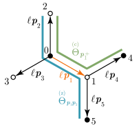
Figure 8: C-dihedral angle $\operatorname{\overset{(c)}{\Theta}}_{\mathbf{p}_{1}^{+}}$ (green) and Z-dihedral angle $\operatorname{\overset{(z)}{\Theta}}_{\mathbf{p}_{1}\mathbf{p}_{2}}$ (blue).

The first order approximation of the dihedral angle is all we need to evaluate the corresponding energy contribution.

Let us denote by

$$\mathbf{q}_{1}=\ell\mathbf{p}_{1}+(\operatorname{\boldsymbol{\mathfrak{u}}}_{1}-\operatorname{\boldsymbol{\mathfrak{u}}}_{0}){{}\mathchoice{\mbox{\boldmath$\displaystyle\mathchar 280\relax$}}{\mbox{\boldmath$\textstyle\mathchar 280\relax$}}{\mbox{\boldmath$\scriptstyle\mathchar 280\relax$}}{\mbox{\boldmath$\scriptscriptstyle\mathchar 280\relax$}}},\quad\mathbf{q}_{2}=\ell\mathbf{p}_{2}+(\operatorname{\boldsymbol{\mathfrak{u}}}_{2}-\operatorname{\boldsymbol{\mathfrak{u}}}_{0}){{}\mathchoice{\mbox{\boldmath$\displaystyle\mathchar 280\relax$}}{\mbox{\boldmath$\textstyle\mathchar 280\relax$}}{\mbox{\boldmath$\scriptstyle\mathchar 280\relax$}}{\mbox{\boldmath$\scriptscriptstyle\mathchar 280\relax$}}},\quad\mathbf{q}_{4}=\ell\mathbf{p}_{4}+(\operatorname{\boldsymbol{\mathfrak{u}}}_{4}-\operatorname{\boldsymbol{\mathfrak{u}}}_{1}){{}\mathchoice{\mbox{\boldmath$\displaystyle\mathchar 280\relax$}}{\mbox{\boldmath$\textstyle\mathchar 280\relax$}}{\mbox{\boldmath$\scriptstyle\mathchar 280\relax$}}{\mbox{\boldmath$\scriptscriptstyle\mathchar 280\relax$}}}$$ (69)

the edge vectors after the deformation. We have that

$$|\sin\Big{(}\operatorname{\overset{(c)}{\Theta}}_{\mathbf{p}_{1}^{+}}({{}\mathchoice{\mbox{\boldmath$\displaystyle\mathchar 280\relax$}}{\mbox{\boldmath$\textstyle\mathchar 280\relax$}}{\mbox{\boldmath$\scriptstyle\mathchar 280\relax$}}{\mbox{\boldmath$\scriptscriptstyle\mathchar 280\relax$}}})\Big{)}|=\frac{|(\mathbf{q}_{1}\times\mathbf{q}_{2})\times(\mathbf{q}_{1}\times\mathbf{q}_{4})|}{|\mathbf{q}_{1}\times\mathbf{q}_{2}||\mathbf{q}_{1}\times\mathbf{q}_{4}|};$$ (70)

it is easy to see that

$$\mathbf{q}_{1}\times\mathbf{q}_{2}=\frac{\sqrt{3}}{2}\ell^{2}\mathbf{e}_{3}+\Big{(}\ell\mathbf{p}_{1}\times(\operatorname{\boldsymbol{\mathfrak{u}}}_{2}-\operatorname{\boldsymbol{\mathfrak{u}}}_{0})-\ell\mathbf{p}_{2}\times(\operatorname{\boldsymbol{\mathfrak{u}}}_{1}-\operatorname{\boldsymbol{\mathfrak{u}}}_{0})\Big{)}{{}\mathchoice{\mbox{\boldmath$\displaystyle\mathchar 280\relax$}}{\mbox{\boldmath$\textstyle\mathchar 280\relax$}}{\mbox{\boldmath$\scriptstyle\mathchar 280\relax$}}{\mbox{\boldmath$\scriptscriptstyle\mathchar 280\relax$}}}+O({{}\mathchoice{\mbox{\boldmath$\displaystyle\mathchar 280\relax$}}{\mbox{\boldmath$\textstyle\mathchar 280\relax$}}{\mbox{\boldmath$\scriptstyle\mathchar 280\relax$}}{\mbox{\boldmath$\scriptscriptstyle\mathchar 280\relax$}}}^{2}),$$ (71)

$$\mathbf{q}_{1}\times\mathbf{q}_{4}=\frac{\sqrt{3}}{2}\ell^{2}\mathbf{e}_{3}+\Big{(}\ell\mathbf{p}_{1}\times(\operatorname{\boldsymbol{\mathfrak{u}}}_{4}-\operatorname{\boldsymbol{\mathfrak{u}}}_{1})-\ell\mathbf{p}_{4}\times(\operatorname{\boldsymbol{\mathfrak{u}}}_{1}-\operatorname{\boldsymbol{\mathfrak{u}}}_{0})\Big{)}{{}\mathchoice{\mbox{\boldmath$\displaystyle\mathchar 280\relax$}}{\mbox{\boldmath$\textstyle\mathchar 280\relax$}}{\mbox{\boldmath$\scriptstyle\mathchar 280\relax$}}{\mbox{\boldmath$\scriptscriptstyle\mathchar 280\relax$}}}+O({{}\mathchoice{\mbox{\boldmath$\displaystyle\mathchar 280\relax$}}{\mbox{\boldmath$\textstyle\mathchar 280\relax$}}{\mbox{\boldmath$\scriptstyle\mathchar 280\relax$}}{\mbox{\boldmath$\scriptscriptstyle\mathchar 280\relax$}}}^{2}),$$

whence

$$(\mathbf{q}_{1}\times\mathbf{q}_{2})\times(\mathbf{q}_{1}\times\mathbf{q}_{4})=\frac{\sqrt{3}}{2}\mathbf{e}_{3} \times\Big{(}\ell\mathbf{p}_{1}\times(\operatorname{\boldsymbol{\mathfrak{u}}}_{4}-\operatorname{\boldsymbol{\mathfrak{u}}}_{1})-\ell\mathbf{p}_{4}\times(\operatorname{\boldsymbol{\mathfrak{u}}}_{1}-\operatorname{\boldsymbol{\mathfrak{u}}}_{0})+$$ (72)

$$+\ell\mathbf{p}_{2}\times(\operatorname{\boldsymbol{\mathfrak{u}}}_{1}-\operatorname{\boldsymbol{\mathfrak{u}}}_{0})-\ell\mathbf{p}_{1}\times(\operatorname{\boldsymbol{\mathfrak{u}}}_{2}-\operatorname{\boldsymbol{\mathfrak{u}}}_{0})\Big{)}{{}\mathchoice{\mbox{\boldmath$\displaystyle\mathchar 280\relax$}}{\mbox{\boldmath$\textstyle\mathchar 280\relax$}}{\mbox{\boldmath$\scriptstyle\mathchar 280\relax$}}{\mbox{\boldmath$\scriptscriptstyle\mathchar 280\relax$}}}+O({{}\mathchoice{\mbox{\boldmath$\displaystyle\mathchar 280\relax$}}{\mbox{\boldmath$\textstyle\mathchar 280\relax$}}{\mbox{\boldmath$\scriptstyle\mathchar 280\relax$}}{\mbox{\boldmath$\scriptscriptstyle\mathchar 280\relax$}}}^{2}).$$

On recalling the identity

$$\mathbf{a}\times(\mathbf{b}\times\mathbf{c})=(\mathbf{a}\cdot\mathbf{b})\mathbf{c}-(\mathbf{a}\cdot\mathbf{c})\mathbf{b},$$ (73)

we obtain:

$$(\mathbf{q}_{1}\times\mathbf{q}_{2})\times(\mathbf{q}_{1}\times\mathbf{q}_{4})=\frac{\sqrt{3}}{2}\ell^{2}\Big{(}2\mathfrak{w}_{1}-\mathfrak{w}_{4}+\mathfrak{w}_{2}-2\mathfrak{w}_{0}\Big{)}\ell\mathbf{p}_{1}{{}\mathchoice{\mbox{\boldmath$\displaystyle\mathchar 280\relax$}}{\mbox{\boldmath$\textstyle\mathchar 280\relax$}}{\mbox{\boldmath$\scriptstyle\mathchar 280\relax$}}{\mbox{\boldmath$\scriptscriptstyle\mathchar 280\relax$}}}+O({{}\mathchoice{\mbox{\boldmath$\displaystyle\mathchar 280\relax$}}{\mbox{\boldmath$\textstyle\mathchar 280\relax$}}{\mbox{\boldmath$\scriptstyle\mathchar 280\relax$}}{\mbox{\boldmath$\scriptscriptstyle\mathchar 280\relax$}}}^{2}),$$ (74)

where we have used the fact that $\mathbf{p}_{4}-\mathbf{p}_{2}(=-\mathbf{p}_{3}-\mathbf{p}_{2})=\mathbf{p}_{1}$ and set $\mathfrak{w}=\operatorname{\boldsymbol{\mathfrak{u}}}\cdot\mathbf{e}_{3}$. Now,

$$|\mathbf{q}_{1}\times\mathbf{q}_{2}|=|\mathbf{q}_{1}\times\mathbf{q}_{2}|=\frac{\sqrt{3}}{2}\ell^{2}+O({{}\mathchoice{\mbox{\boldmath$\displaystyle\mathchar 280\relax$}}{\mbox{\boldmath$\textstyle\mathchar 280\relax$}}{\mbox{\boldmath$\scriptstyle\mathchar 280\relax$}}{\mbox{\boldmath$\scriptscriptstyle\mathchar 280\relax$}}}^{2}),$$ (75)

whence

$$|\sin\Big{(}\operatorname{\overset{(c)}{\Theta}}_{\mathbf{p}_{1}^{+}}({{}\mathchoice{\mbox{\boldmath$\displaystyle\mathchar 280\relax$}}{\mbox{\boldmath$\textstyle\mathchar 280\relax$}}{\mbox{\boldmath$\scriptstyle\mathchar 280\relax$}}{\mbox{\boldmath$\scriptscriptstyle\mathchar 280\relax$}}})\Big{)}|=|{{}\mathchoice{\mbox{\boldmath$\displaystyle\mathchar 270\relax$}}{\mbox{\boldmath$\textstyle\mathchar 270\relax$}}{\mbox{\boldmath$\scriptstyle\mathchar 270\relax$}}{\mbox{\boldmath$\scriptscriptstyle\mathchar 270\relax$}}}\operatorname{\overset{(c)}{\Theta}}_{\mathbf{p}_{1}^{+}}|{{}\mathchoice{\mbox{\boldmath$\displaystyle\mathchar 280\relax$}}{\mbox{\boldmath$\textstyle\mathchar 280\relax$}}{\mbox{\boldmath$\scriptstyle\mathchar 280\relax$}}{\mbox{\boldmath$\scriptscriptstyle\mathchar 280\relax$}}}+O({{}\mathchoice{\mbox{\boldmath$\displaystyle\mathchar 280\relax$}}{\mbox{\boldmath$\textstyle\mathchar 280\relax$}}{\mbox{\boldmath$\scriptstyle\mathchar 280\relax$}}{\mbox{\boldmath$\scriptscriptstyle\mathchar 280\relax$}}}^{2})=\frac{2\sqrt{3}}{3\ell}\Big{|}2\mathfrak{w}_{1}-\mathfrak{w}_{4}+\mathfrak{w}_{2}-2\mathfrak{w}_{0}\Big{|}{{}\mathchoice{\mbox{\boldmath$\displaystyle\mathchar 280\relax$}}{\mbox{\boldmath$\textstyle\mathchar 280\relax$}}{\mbox{\boldmath$\scriptstyle\mathchar 280\relax$}}{\mbox{\boldmath$\scriptscriptstyle\mathchar 280\relax$}}}+O({{}\mathchoice{\mbox{\boldmath$\displaystyle\mathchar 280\relax$}}{\mbox{\boldmath$\textstyle\mathchar 280\relax$}}{\mbox{\boldmath$\scriptstyle\mathchar 280\relax$}}{\mbox{\boldmath$\scriptscriptstyle\mathchar 280\relax$}}}^{2}).$$ (76)

Thus, on recalling that $w=\mathfrak{w}{{}\mathchoice{\mbox{\boldmath$\displaystyle\mathchar 280\relax$}}{\mbox{\boldmath$\textstyle\mathchar 280\relax$}}{\mbox{\boldmath$\scriptstyle\mathchar 280\relax$}}{\mbox{\boldmath$\scriptscriptstyle\mathchar 280\relax$}}}$, we conclude that

$${{}\mathchoice{\mbox{\boldmath$\displaystyle\mathchar 270\relax$}}{\mbox{\boldmath$\textstyle\mathchar 270\relax$}}{\mbox{\boldmath$\scriptstyle\mathchar 270\relax$}}{\mbox{\boldmath$\scriptscriptstyle\mathchar 270\relax$}}}\operatorname{\overset{(c)}{\Theta}}_{\mathbf{p}_{1}^{+}}=\frac{2\sqrt{3}}{3\ell}\Big{(}2w_{1}-w_{4}+w_{2}-2w_{0}\Big{)}.$$ (77)

For a generic C-dihedral angle centered in $\mathbf{p}_{i}$, we get

$${{}\mathchoice{\mbox{\boldmath$\displaystyle\mathchar 270\relax$}}{\mbox{\boldmath$\textstyle\mathchar 270\relax$}}{\mbox{\boldmath$\scriptstyle\mathchar 270\relax$}}{\mbox{\boldmath$\scriptscriptstyle\mathchar 270\relax$}}}\operatorname{\overset{(c)}{\Theta}}_{\mathbf{p}_{i}^{+}}(\mathbf{x}^{\ell})=\frac{2\sqrt{3}}{3\ell}[2w(\mathbf{x}^{\ell})-w(\mathbf{x}^{\ell}+\ell\mathbf{p}_{i+1})+w(\mathbf{x}^{\ell}+\ell\mathbf{p}_{i}-\ell\mathbf{p}_{i+2})-2w(\mathbf{x}^{\ell}+\ell\mathbf{p}_{i})],$$ (78)

$${{}\mathchoice{\mbox{\boldmath$\displaystyle\mathchar 270\relax$}}{\mbox{\boldmath$\textstyle\mathchar 270\relax$}}{\mbox{\boldmath$\scriptstyle\mathchar 270\relax$}}{\mbox{\boldmath$\scriptscriptstyle\mathchar 270\relax$}}}\operatorname{\overset{(c)}{\Theta}}_{\mathbf{p}_{i}^{-}}(\mathbf{x}^{\ell})=-\frac{2\sqrt{3}}{3\ell}[2w(\mathbf{x}^{\ell})-w(\mathbf{x}^{\ell}+\ell\mathbf{p}_{i+2})+w(\mathbf{x}^{\ell}+\ell\mathbf{p}_{i}-\ell\mathbf{p}_{i+1})-2w(\mathbf{x}^{\ell}+\ell\mathbf{p}_{i})].$$

For the Z-dihedral angle $\operatorname{\overset{(z)}{\Theta}}_{\mathbf{p}_{1}\mathbf{p}_{2}}$, we introduce the vector

$$\mathbf{q}_{5}=\ell\mathbf{p}_{5}+(\operatorname{\boldsymbol{\mathfrak{u}}}_{5}-\operatorname{\boldsymbol{\mathfrak{u}}}_{1}){{}\mathchoice{\mbox{\boldmath$\displaystyle\mathchar 280\relax$}}{\mbox{\boldmath$\textstyle\mathchar 280\relax$}}{\mbox{\boldmath$\scriptstyle\mathchar 280\relax$}}{\mbox{\boldmath$\scriptscriptstyle\mathchar 280\relax$}}},$$

image of $\mathbf{p}_{5}$ under the deformation. We have that

$$|\sin\operatorname{\overset{(z)}{\Theta}}_{\mathbf{p}_{1}\mathbf{p}_{2}}|=\frac{|(\mathbf{q}_{1}\times\mathbf{q}_{2})\times(\mathbf{q}_{5}\times\mathbf{q}_{1})|}{|\mathbf{q}_{1}\times\mathbf{q}_{2}||\mathbf{q}_{5}\times\mathbf{q}_{1}|},$$ (79)

and

$$\mathbf{q}_{5}\times\mathbf{q}_{1}=\frac{\sqrt{3}}{2}\ell^{2}\mathbf{e}_{3}+\Big{(}\ell\mathbf{p}_{5}\times(\operatorname{\boldsymbol{\mathfrak{u}}}_{1}-\operatorname{\boldsymbol{\mathfrak{u}}}_{0})-\ell\mathbf{p}_{1}\times(\operatorname{\boldsymbol{\mathfrak{u}}}_{5}-\operatorname{\boldsymbol{\mathfrak{u}}}_{1})\Big{)}{{}\mathchoice{\mbox{\boldmath$\displaystyle\mathchar 280\relax$}}{\mbox{\boldmath$\textstyle\mathchar 280\relax$}}{\mbox{\boldmath$\scriptstyle\mathchar 280\relax$}}{\mbox{\boldmath$\scriptscriptstyle\mathchar 280\relax$}}}+O({{}\mathchoice{\mbox{\boldmath$\displaystyle\mathchar 280\relax$}}{\mbox{\boldmath$\textstyle\mathchar 280\relax$}}{\mbox{\boldmath$\scriptstyle\mathchar 280\relax$}}{\mbox{\boldmath$\scriptscriptstyle\mathchar 280\relax$}}}^{2}),$$ (80)

whence

$$(\mathbf{q}_{1}\times\mathbf{q}_{2})\times(\mathbf{q}_{5}\times\mathbf{q}_{1})=\frac{\sqrt{3}}{2}\ell^{2}\mathbf{e}_{3} \times\Big{(}\ell\mathbf{p}_{5}\times(\operatorname{\boldsymbol{\mathfrak{u}}}_{1}-\operatorname{\boldsymbol{\mathfrak{u}}}_{0})-\ell\mathbf{p}_{1}\times(\operatorname{\boldsymbol{\mathfrak{u}}}_{5}-\operatorname{\boldsymbol{\mathfrak{u}}}_{1})$$ (81)

$$+\ell\mathbf{p}_{2}\times(\operatorname{\boldsymbol{\mathfrak{u}}}_{1}-\operatorname{\boldsymbol{\mathfrak{u}}}_{0})-\ell\mathbf{p}_{1}\times(\operatorname{\boldsymbol{\mathfrak{u}}}_{2}-\operatorname{\boldsymbol{\mathfrak{u}}}_{0})\Big{)}{{}\mathchoice{\mbox{\boldmath$\displaystyle\mathchar 280\relax$}}{\mbox{\boldmath$\textstyle\mathchar 280\relax$}}{\mbox{\boldmath$\scriptstyle\mathchar 280\relax$}}{\mbox{\boldmath$\scriptscriptstyle\mathchar 280\relax$}}}+O({{}\mathchoice{\mbox{\boldmath$\displaystyle\mathchar 280\relax$}}{\mbox{\boldmath$\textstyle\mathchar 280\relax$}}{\mbox{\boldmath$\scriptstyle\mathchar 280\relax$}}{\mbox{\boldmath$\scriptscriptstyle\mathchar 280\relax$}}}^{2}).$$

Again, on making use of (73) and recalling that $\mathbf{p}_{5}=-\mathbf{p}_{2}$, we obtain:

$$(\mathbf{q}_{1}\times\mathbf{q}_{2})\times(\mathbf{q}_{5}\times\mathbf{q}_{1})=\frac{\sqrt{3}}{2}\ell^{2}(\mathfrak{w}_{5}-\mathfrak{w}_{1}+\mathfrak{w}_{2}-\mathfrak{w}_{0}){{}\mathchoice{\mbox{\boldmath$\displaystyle\mathchar 280\relax$}}{\mbox{\boldmath$\textstyle\mathchar 280\relax$}}{\mbox{\boldmath$\scriptstyle\mathchar 280\relax$}}{\mbox{\boldmath$\scriptscriptstyle\mathchar 280\relax$}}}+O({{}\mathchoice{\mbox{\boldmath$\displaystyle\mathchar 280\relax$}}{\mbox{\boldmath$\textstyle\mathchar 280\relax$}}{\mbox{\boldmath$\scriptstyle\mathchar 280\relax$}}{\mbox{\boldmath$\scriptscriptstyle\mathchar 280\relax$}}}^{2}).$$ (82)

On noticing that $|\mathbf{q}_{5}\times\mathbf{q}_{1}|=\frac{\sqrt{3}}{2}\ell^{2}+O({{}\mathchoice{\mbox{\boldmath$\displaystyle\mathchar 280\relax$}}{\mbox{\boldmath$\textstyle\mathchar 280\relax$}}{\mbox{\boldmath$\scriptstyle\mathchar 280\relax$}}{\mbox{\boldmath$\scriptscriptstyle\mathchar 280\relax$}}}^{2})$, we get

$$|\sin\operatorname{\overset{(z)}{\Theta}}_{\mathbf{p}_{1}\mathbf{p}_{2}}|=|{{}\mathchoice{\mbox{\boldmath$\displaystyle\mathchar 270\relax$}}{\mbox{\boldmath$\textstyle\mathchar 270\relax$}}{\mbox{\boldmath$\scriptstyle\mathchar 270\relax$}}{\mbox{\boldmath$\scriptscriptstyle\mathchar 270\relax$}}}\operatorname{\overset{(z)}{\Theta}}_{\mathbf{p}_{1}\mathbf{p}_{2}}|{{}\mathchoice{\mbox{\boldmath$\displaystyle\mathchar 280\relax$}}{\mbox{\boldmath$\textstyle\mathchar 280\relax$}}{\mbox{\boldmath$\scriptstyle\mathchar 280\relax$}}{\mbox{\boldmath$\scriptscriptstyle\mathchar 280\relax$}}}+O({{}\mathchoice{\mbox{\boldmath$\displaystyle\mathchar 280\relax$}}{\mbox{\boldmath$\textstyle\mathchar 280\relax$}}{\mbox{\boldmath$\scriptstyle\mathchar 280\relax$}}{\mbox{\boldmath$\scriptscriptstyle\mathchar 280\relax$}}}^{2})=\frac{2\sqrt{3}}{3\ell}\Big{|}\mathfrak{w}_{5}-\mathfrak{w}_{1}+\mathfrak{w}_{2}-\mathfrak{w}_{0}\Big{|}{{}\mathchoice{\mbox{\boldmath$\displaystyle\mathchar 280\relax$}}{\mbox{\boldmath$\textstyle\mathchar 280\relax$}}{\mbox{\boldmath$\scriptstyle\mathchar 280\relax$}}{\mbox{\boldmath$\scriptscriptstyle\mathchar 280\relax$}}}+O({{}\mathchoice{\mbox{\boldmath$\displaystyle\mathchar 280\relax$}}{\mbox{\boldmath$\textstyle\mathchar 280\relax$}}{\mbox{\boldmath$\scriptstyle\mathchar 280\relax$}}{\mbox{\boldmath$\scriptscriptstyle\mathchar 280\relax$}}}^{2}),$$ (83)

whence

$${{}\mathchoice{\mbox{\boldmath$\displaystyle\mathchar 270\relax$}}{\mbox{\boldmath$\textstyle\mathchar 270\relax$}}{\mbox{\boldmath$\scriptstyle\mathchar 270\relax$}}{\mbox{\boldmath$\scriptscriptstyle\mathchar 270\relax$}}}\operatorname{\overset{(z)}{\Theta}}_{\mathbf{p}_{1}\mathbf{p}_{2}}=\frac{2\sqrt{3}}{3\ell}\Big{(}w_{5}-w_{1}+w_{2}-w_{0}\Big{)}.$$ (84)

For a generic Z-dihedral angle centered in $\mathbf{p}_{i}$, we get

$${{}\mathchoice{\mbox{\boldmath$\displaystyle\mathchar 270\relax$}}{\mbox{\boldmath$\textstyle\mathchar 270\relax$}}{\mbox{\boldmath$\scriptstyle\mathchar 270\relax$}}{\mbox{\boldmath$\scriptscriptstyle\mathchar 270\relax$}}}\operatorname{\overset{(z)}{\Theta}}_{\mathbf{p}_{i}\mathbf{p}_{i+1}}(\mathbf{x}^{\ell})=\frac{2\sqrt{3}}{3\ell}[w(\mathbf{x}^{\ell}+\ell\mathbf{p}_{i}-\ell\mathbf{p}_{i+1})-w(\mathbf{x}^{\ell}+\ell\mathbf{p}_{i})+w(\mathbf{x}^{\ell}+\ell\mathbf{p}_{i+1})-w(\mathbf{x}^{\ell})],$$ (85)

$${{}\mathchoice{\mbox{\boldmath$\displaystyle\mathchar 270\relax$}}{\mbox{\boldmath$\textstyle\mathchar 270\relax$}}{\mbox{\boldmath$\scriptstyle\mathchar 270\relax$}}{\mbox{\boldmath$\scriptscriptstyle\mathchar 270\relax$}}}\operatorname{\overset{(z)}{\Theta}}_{\mathbf{p}_{i}\mathbf{p}_{i+2}}(\mathbf{x}^{\ell})=\frac{2\sqrt{3}}{3\ell}[w(\mathbf{x}^{\ell}+\ell\mathbf{p}_{i}-\ell\mathbf{p}_{i+2})-w(\mathbf{x}^{\ell}+\ell\mathbf{p}_{i})+w(\mathbf{x}^{\ell}+\ell\mathbf{p}_{i+2})-w(\mathbf{x}^{\ell})].$$

A.3 Deduction of the continuum limits $\mathcal{U}^{\mathcal{C}}_{0}$ and $\mathcal{U}^{(s)}_{0}$

In this Appendix we give a justification of (32) and (33) following the lines outlined in Section 5 for the derivation of the continuum limit of the Z-dihedral energy.

As in Section 5, in place of a function $w:(L_{1}(\ell)\cup L_{2}(\ell))\cap\Omega\to\mathbb{R}$, we consider a twice continuously differentiable function $w:\Omega\to\mathbb{R}$. We first consider the contribution due to the C-dihedra. Momentarily, to keep the notation compact, we set

$$\mathbf{g}:=\nabla w(\mathbf{x}^{\ell}),\qquad\mathbf{H}:=\nabla^{2}w(\mathbf{x}^{\ell}).$$ (86)

By Taylor’s expansion we have

$$-w(\mathbf{x}^{\ell}+\ell\mathbf{p}_{i+1}) =-w(\mathbf{x}^{\ell})-\ell\mathbf{g}\cdot\mathbf{p}_{i+1}-\frac{1}{2}\ell^{2}\mathbf{H}\mathbf{p}_{i+1}\cdot\mathbf{p}_{i+1}+o(\ell^{2})$$

$$w(\mathbf{x}^{\ell}+\ell\mathbf{p}_{i}-\ell\mathbf{p}_{i+2}) =w(\mathbf{x}^{\ell})+\ell\mathbf{g}\cdot(\mathbf{p}_{i}-\mathbf{p}_{i+2})+\frac{1}{2}\ell^{2}\mathbf{H}(\mathbf{p}_{i}-\mathbf{p}_{i+2})\cdot(\mathbf{p}_{i}-\mathbf{p}_{i+2})+o(\ell^{2})$$

$$-2w(\mathbf{x}^{\ell}+\ell\mathbf{p}_{i}) =-2w(\mathbf{x}^{\ell})-2\ell\mathbf{g}\cdot\mathbf{p}_{i}-\ell^{2}\mathbf{H}\mathbf{p}_{i}\cdot\mathbf{p}_{i}+o(\ell^{2}).$$

Thence, since $\mathbf{p}_{1}+\mathbf{p}_{2}+\mathbf{p}_{3}=\mathbf{0}$, we find from (18) that

$${{}\mathchoice{\mbox{\boldmath$\displaystyle\mathchar 270\relax$}}{\mbox{\boldmath$\textstyle\mathchar 270\relax$}}{\mbox{\boldmath$\scriptstyle\mathchar 270\relax$}}{\mbox{\boldmath$\scriptscriptstyle\mathchar 270\relax$}}}\operatorname{\overset{(c)}{\Theta}}_{\mathbf{p}_{i}^{+}}(\mathbf{x}^{\ell}) =\frac{2\sqrt{3}}{3\ell}[2w(\mathbf{x}^{\ell})-w(\mathbf{x}^{\ell}+\ell\mathbf{p}_{i+1})+w(\mathbf{x}^{\ell}+\ell\mathbf{p}_{i}-\ell\mathbf{p}_{i+2})-2w(\mathbf{x}^{\ell}+\ell\mathbf{p}_{i})]$$

$$=\frac{\sqrt{3}\ell}{3}[-\mathbf{H}\mathbf{p}_{i+1}\cdot\mathbf{p}_{i+1}+\mathbf{H}(\mathbf{p}_{i}-\mathbf{p}_{i+2})\cdot(\mathbf{p}_{i}-\mathbf{p}_{i+2})-2\mathbf{H}\mathbf{p}_{i}\cdot\mathbf{p}_{i})]+o(\ell)$$

and, by substituting $\mathbf{p}_{i+2}=-(\mathbf{p}_{i}+\mathbf{p}_{i+1})$, we eventually get

$${{}\mathchoice{\mbox{\boldmath$\displaystyle\mathchar 270\relax$}}{\mbox{\boldmath$\textstyle\mathchar 270\relax$}}{\mbox{\boldmath$\scriptstyle\mathchar 270\relax$}}{\mbox{\boldmath$\scriptscriptstyle\mathchar 270\relax$}}}\operatorname{\overset{(c)}{\Theta}}_{\mathbf{p}_{i}^{+}}(\mathbf{x}^{\ell}) =\frac{\sqrt{3}\ell}{3}[-\mathbf{H}\mathbf{p}_{i+1}\cdot\mathbf{p}_{i+1}+\mathbf{H}(2\mathbf{p}_{i}+\mathbf{p}_{i+1})\cdot(2\mathbf{p}_{i}+\mathbf{p}_{i+1})-2\mathbf{H}\mathbf{p}_{i}\cdot\mathbf{p}_{i}]+o(\ell)$$

$$=\frac{4\sqrt{3}\ell}{3}[\mathbf{H}\mathbf{p}_{i}\cdot(\frac{1}{2}\mathbf{p}_{i}+\mathbf{p}_{i+1})]+o(\ell)$$

$$={2\ell}\mathbf{H}\mathbf{p}_{i}\cdot\mathbf{p}_{i}^{\perp}+o(\ell)={2\ell}\partial^{2}_{\mathbf{p}_{i}\mathbf{p}_{i}^{\perp}}w(\mathbf{x}^{\ell})+o(\ell).$$ (87)

where $\mathbf{p}_{i}^{\perp}$ is defined in (13). Similarly, we also find that

$${{}\mathchoice{\mbox{\boldmath$\displaystyle\mathchar 270\relax$}}{\mbox{\boldmath$\textstyle\mathchar 270\relax$}}{\mbox{\boldmath$\scriptstyle\mathchar 270\relax$}}{\mbox{\boldmath$\scriptscriptstyle\mathchar 270\relax$}}}\operatorname{\overset{(c)}{\Theta}}_{\mathbf{p}_{i}^{-}}(\mathbf{x}^{\ell})={2\ell}\partial^{2}_{\mathbf{p}_{i}\mathbf{p}_{i}^{\perp}}w(\mathbf{x}^{\ell})+o(\ell).$$ (88)

With the same steps taken in the study of the Z-dihedral energy we now derive the limit of the C-dihedral energy. With the expressions of the change of the C-dihedra (87) and (88), we can rewrite the C-dihedral energy, see (37), as

$$\mathcal{U}^{\mathcal{C}}_{\ell} =\frac{1}{2}k^{\mathcal{C}}\,\sum_{\mathbf{x}^{\ell}\in L_{2}(\ell)\cap\Omega}\sum_{i=1}^{3}\Bigg{(}{{}\mathchoice{\mbox{\boldmath$\displaystyle\mathchar 270\relax$}}{\mbox{\boldmath$\textstyle\mathchar 270\relax$}}{\mbox{\boldmath$\scriptstyle\mathchar 270\relax$}}{\mbox{\boldmath$\scriptscriptstyle\mathchar 270\relax$}}}\operatorname{\overset{(c)}{\Theta}}_{\mathbf{p}_{i}^{+}}(\mathbf{x}^{\ell})\Bigg{)}^{2}+\Bigg{(}{{}\mathchoice{\mbox{\boldmath$\displaystyle\mathchar 270\relax$}}{\mbox{\boldmath$\textstyle\mathchar 270\relax$}}{\mbox{\boldmath$\scriptstyle\mathchar 270\relax$}}{\mbox{\boldmath$\scriptscriptstyle\mathchar 270\relax$}}}\operatorname{\overset{(c)}{\Theta}}_{\mathbf{p}_{i}^{-}}(\mathbf{x}^{\ell})\Bigg{)}^{2}$$

$$=\frac{1}{2}8\ell^{2}k^{\mathcal{C}}\,\sum_{\mathbf{x}^{\ell}\in L_{2}(\ell)\cap\Omega}\sum_{i=1}^{3}\Big{(}\partial^{2}_{\mathbf{p}_{i}\mathbf{p}_{i}^{\perp}}w(\mathbf{x}^{\ell})\Big{)}^{2}+o(\ell^{2})$$

$$=\frac{1}{2}\frac{16\sqrt{3}}{9}k^{\mathcal{C}}\,\sum_{\mathbf{x}^{\ell}\in L_{2}(\ell)\cap\Omega}\sum_{i=1}^{3}\Big{(}\partial^{2}_{\mathbf{p}_{i}\mathbf{p}_{i}^{\perp}}w(\mathbf{x}^{\ell})\Big{)}^{2}|E^{\ell}(\mathbf{x}^{\ell})|+o(\ell^{2})$$

$$=\frac{1}{2}\frac{16\sqrt{3}}{9}k^{\mathcal{C}}\int_{\Omega}W^{\mathcal{C}}_{\ell}(\mathbf{x})\,d\mathbf{x}+o(\ell^{2}),$$

where the function

$$W^{\mathcal{C}}_{\ell}(\mathbf{x}):=\sum_{\mathbf{x}^{\ell}\in L_{2}(\ell)\cap\Omega}\sum_{i=1}^{3}\Big{(}\partial^{2}_{\mathbf{p}_{i}\mathbf{p}_{i}^{\perp}}w(\mathbf{x}^{\ell})\Big{)}^{2}{{}\mathchoice{\mbox{\boldmath$\displaystyle\mathchar 287\relax$}}{\mbox{\boldmath$\textstyle\mathchar 287\relax$}}{\mbox{\boldmath$\scriptstyle\mathchar 287\relax$}}{\mbox{\boldmath$\scriptscriptstyle\mathchar 287\relax$}}}_{E^{\ell}(\mathbf{x}^{\ell})}(\mathbf{x})$$

converges to $\sum_{i=1}^{3}\Big{(}\partial^{2}_{\mathbf{p}_{i}\mathbf{p}_{i}^{\perp}}w\Big{)}^{2}$, as $\ell$ goes to zero. Thus,

$$\lim_{\ell\to 0}\mathcal{U}^{\mathcal{C}}_{\ell}=\frac{1}{2}\frac{16\sqrt{3}}{9}k^{\mathcal{C}}\int_{\Omega}\sum_{i=1}^{3}\Big{(}\partial^{2}_{\mathbf{p}_{i}\mathbf{p}_{i}^{\perp}}w\Big{)}^{2}\,d\mathbf{x}=:\mathcal{U}^{\mathcal{C}}_{0}(w),$$ (89)

which is (32).

We now compute the limit of the self-energy. By Taylor’s expansion, with the notation introduced in (86), and taking into account that $\mathbf{p}_{1}+\mathbf{p}_{2}+\mathbf{p}_{3}=\mathbf{0}$, we find

$$\sum_{i}{{}\mathchoice{\mbox{\boldmath$\displaystyle\mathchar 270\relax$}}{\mbox{\boldmath$\textstyle\mathchar 270\relax$}}{\mbox{\boldmath$\scriptstyle\mathchar 270\relax$}}{\mbox{\boldmath$\scriptscriptstyle\mathchar 270\relax$}}}{{}\mathchoice{\mbox{\boldmath$\displaystyle\mathchar 291\relax$}}{\mbox{\boldmath$\textstyle\mathchar 291\relax$}}{\mbox{\boldmath$\scriptstyle\mathchar 291\relax$}}{\mbox{\boldmath$\scriptscriptstyle\mathchar 291\relax$}}}_{i}(\mathbf{x}^{\ell}) =-\frac{3\sqrt{3}}{\ell^{2}}[\frac{1}{3}\sum_{i=1}^{3}w(\mathbf{x}^{\ell}+\ell\mathbf{p}_{i})-w(\mathbf{x}^{\ell})]^{2}$$

$$=-\frac{3\sqrt{3}}{\ell^{2}}\frac{\ell^{4}}{36}(\mathbf{H}\mathbf{p}_{1}\cdot\mathbf{p}_{1}+\mathbf{H}\mathbf{p}_{2}\cdot\mathbf{p}_{2}+\mathbf{H}\mathbf{p}_{3}\cdot\mathbf{p}_{3})^{2}+o(\ell^{2})$$

$$=-\frac{3\sqrt{3}}{\ell^{2}}\frac{\ell^{4}}{9}(\mathbf{H}\mathbf{p}_{1}\cdot\mathbf{p}_{1}+\mathbf{H}\mathbf{p}_{2}\cdot\mathbf{p}_{2}+\mathbf{H}\mathbf{p}_{1}\cdot\mathbf{p}_{2})^{2}+o(\ell^{2})$$

$$=-\frac{\sqrt{3}}{3}{\ell^{2}}\Big{(}\partial^{2}_{\mathbf{p}_{1}\mathbf{p}_{1}}w(\mathbf{x}^{\ell})+\partial^{2}_{\mathbf{p}_{2}\mathbf{p}_{2}}w(\mathbf{x}^{\ell})+\partial^{2}_{\mathbf{p}_{1}\mathbf{p}_{2}}w(\mathbf{x}^{\ell})\Big{)}^{2}+o(\ell^{2}).$$ (90)

With this expression the self-energy (22) takes the form

$$\mathcal{U}^{(s)}_{\ell} =\sum_{\mathbf{x}^{\ell}\in(L_{1}(\ell)\cup L_{2}(\ell))\cap\Omega}{{}\mathchoice{\mbox{\boldmath$\displaystyle\mathchar 284\relax$}}{\mbox{\boldmath$\textstyle\mathchar 284\relax$}}{\mbox{\boldmath$\scriptstyle\mathchar 284\relax$}}{\mbox{\boldmath$\scriptscriptstyle\mathchar 284\relax$}}}_{0}\sum_{i=1}^{3}{{}\mathchoice{\mbox{\boldmath$\displaystyle\mathchar 270\relax$}}{\mbox{\boldmath$\textstyle\mathchar 270\relax$}}{\mbox{\boldmath$\scriptstyle\mathchar 270\relax$}}{\mbox{\boldmath$\scriptscriptstyle\mathchar 270\relax$}}}{{}\mathchoice{\mbox{\boldmath$\displaystyle\mathchar 291\relax$}}{\mbox{\boldmath$\textstyle\mathchar 291\relax$}}{\mbox{\boldmath$\scriptstyle\mathchar 291\relax$}}{\mbox{\boldmath$\scriptscriptstyle\mathchar 291\relax$}}}_{i}(\mathbf{x}^{\ell})$$

$$=-\frac{\sqrt{3}}{3}{{}\mathchoice{\mbox{\boldmath$\displaystyle\mathchar 284\relax$}}{\mbox{\boldmath$\textstyle\mathchar 284\relax$}}{\mbox{\boldmath$\scriptstyle\mathchar 284\relax$}}{\mbox{\boldmath$\scriptscriptstyle\mathchar 284\relax$}}}_{0}{\ell^{2}}\sum_{\mathbf{x}^{\ell}\in(L_{1}(\ell)\cup L_{2}(\ell))\cap\Omega}\Big{(}\partial^{2}_{\mathbf{p}_{1}\mathbf{p}_{1}}w(\mathbf{x}^{\ell})+\partial^{2}_{\mathbf{p}_{2}\mathbf{p}_{2}}w(\mathbf{x}^{\ell})+\partial^{2}_{\mathbf{p}_{1}\mathbf{p}_{2}}w(\mathbf{x}^{\ell})\Big{)}^{2}+o(\ell^{2}).$$

Since the sum is over the points of both lattices, whereas in the previous cases the sum was only over the nodes of $L_{2}(\ell)$, we cannot use the hexagons $E^{\ell}(\mathbf{x}^{\ell})$ earlier introduced. Let $T^{\ell}(\mathbf{x}^{\ell})$ be the triangle centered at $\mathbf{x}^{\ell}$ of side $\sqrt{3}\ell$ as depicted in Figure 9.

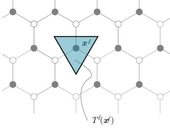
Figure 9: Triangulation $T^{\ell}(\mathbf{x}^{\ell})$

Let

$$W^{{}\mathchoice{\mbox{\boldmath$\displaystyle\mathchar 291\relax$}}{\mbox{\boldmath$\textstyle\mathchar 291\relax$}}{\mbox{\boldmath$\scriptstyle\mathchar 291\relax$}}{\mbox{\boldmath$\scriptscriptstyle\mathchar 291\relax$}}}_{\ell}(\mathbf{x}):=\sum_{\mathbf{x}^{\ell}\in(L_{1}(\ell)\cup L_{2}(\ell))\cap\Omega}\Big{(}\partial^{2}_{\mathbf{p}_{1}\mathbf{p}_{1}}w(\mathbf{x}^{\ell})+\partial^{2}_{\mathbf{p}_{2}\mathbf{p}_{2}}w(\mathbf{x}^{\ell})+\partial^{2}_{\mathbf{p}_{1}\mathbf{p}_{2}}w(\mathbf{x}^{\ell})\Big{)}^{2}{{}\mathchoice{\mbox{\boldmath$\displaystyle\mathchar 287\relax$}}{\mbox{\boldmath$\textstyle\mathchar 287\relax$}}{\mbox{\boldmath$\scriptstyle\mathchar 287\relax$}}{\mbox{\boldmath$\scriptscriptstyle\mathchar 287\relax$}}}_{T^{\ell}(\mathbf{x}^{\ell})}(\mathbf{x})$$

and note that the area of $T^{\ell}(\mathbf{x}^{\ell})$ is $|T^{\ell}(\mathbf{x}^{\ell})|=\frac{3\sqrt{3}}{4}\ell^{2}$. The self-energy rewrites as

$$\mathcal{U}^{(s)}_{\ell} =-\frac{4}{9}{{}\mathchoice{\mbox{\boldmath$\displaystyle\mathchar 284\relax$}}{\mbox{\boldmath$\textstyle\mathchar 284\relax$}}{\mbox{\boldmath$\scriptstyle\mathchar 284\relax$}}{\mbox{\boldmath$\scriptscriptstyle\mathchar 284\relax$}}}_{0}\sum_{\mathbf{x}^{\ell}\in(L_{1}(\ell)\cup L_{2}(\ell))\cap\Omega}\Big{(}\partial^{2}_{\mathbf{p}_{1}\mathbf{p}_{1}}w(\mathbf{x}^{\ell})+\partial^{2}_{\mathbf{p}_{2}\mathbf{p}_{2}}w(\mathbf{x}^{\ell})+\partial^{2}_{\mathbf{p}_{1}\mathbf{p}_{2}}w(\mathbf{x}^{\ell})\Big{)}^{2}|T^{\ell}(\mathbf{x}^{\ell})|$$

$$\quad+o(\ell^{2})$$

$$=-\frac{4}{9}{{}\mathchoice{\mbox{\boldmath$\displaystyle\mathchar 284\relax$}}{\mbox{\boldmath$\textstyle\mathchar 284\relax$}}{\mbox{\boldmath$\scriptstyle\mathchar 284\relax$}}{\mbox{\boldmath$\scriptscriptstyle\mathchar 284\relax$}}}_{0}\int_{\Omega}W^{{}\mathchoice{\mbox{\boldmath$\displaystyle\mathchar 291\relax$}}{\mbox{\boldmath$\textstyle\mathchar 291\relax$}}{\mbox{\boldmath$\scriptstyle\mathchar 291\relax$}}{\mbox{\boldmath$\scriptscriptstyle\mathchar 291\relax$}}}_{\ell}(\mathbf{x})\,d\mathbf{x}+o(\ell^{2}).$$

Since $W^{{}\mathchoice{\mbox{\boldmath$\displaystyle\mathchar 291\relax$}}{\mbox{\boldmath$\textstyle\mathchar 291\relax$}}{\mbox{\boldmath$\scriptstyle\mathchar 291\relax$}}{\mbox{\boldmath$\scriptscriptstyle\mathchar 291\relax$}}}_{\ell}$ converges to $(\partial^{2}_{\mathbf{p}_{1}\mathbf{p}_{1}}w+\partial^{2}_{\mathbf{p}_{2}\mathbf{p}_{2}}w+\partial^{2}_{\mathbf{p}_{1}\mathbf{p}_{2}}w\Big{)}^{2}$ as $\ell$ goes to zero, we find

$$\lim_{\ell\to 0}\mathcal{U}^{(s)}_{\ell}=-\frac{4}{9}{{}\mathchoice{\mbox{\boldmath$\displaystyle\mathchar 284\relax$}}{\mbox{\boldmath$\textstyle\mathchar 284\relax$}}{\mbox{\boldmath$\scriptstyle\mathchar 284\relax$}}{\mbox{\boldmath$\scriptscriptstyle\mathchar 284\relax$}}}_{0}\int_{\Omega}(\partial^{2}_{\mathbf{p}_{1}\mathbf{p}_{1}}w+\partial^{2}_{\mathbf{p}_{2}\mathbf{p}_{2}}w+\partial^{2}_{\mathbf{p}_{1}\mathbf{p}_{2}}w\Big{)}^{2}\,d\mathbf{x}=:\mathcal{U}^{(s)}_{0}(w),$$ (91)

which is (33).

References

- [1] D. Akinwande, C.J. Brennan, J.S. Bunch, P. Egberts, J.R. Felts, H. Gao, R. Huang, J.-S. Kim, T. Li, Y. Li, K.M. Liechti, N. Lu, H.S. Park, E.J. Reed, P. Wang, B.I. Yakobson, T. Zhang, Y.-W. Zhang, Y. Zhou, and Zhu Y. A review on mechanics and mechanical properties of 2d materials - graphene and beyond. Preprint at arXiv:1609.07187.
- [2] R. Alessi, A. Favata, and A. Micheletti. Pressurized CNTs under tension: A finite-deformation lattice model. Compos. Part B Eng., in press, http://dx.doi.org/10.1016/j.compositesb.2016.10.006.
- [3] M. Arroyo and T. Belytschko. An atomistic-based finite deformation membrane for single layer crystalline films. J. Mech. Phys. Solids, 50(9):1941 – 1977, 2002.
- [4] M. Arroyo and T. Belytschko. Finite crystal elasticity of carbon nanotubes based on the exponential cauchy-born rule. Phys. Rev. B, 69:115415, 2004.
- [5] C. Bajaj, A. Favata, and P. Podio-Guidugli. On a nanoscopically-informed shell theory of carbon nanotubes. Europ. J. Mech. A/Solids, 42:137–157, 2013.
- [6] D.W. Brenner, O.A. Shenderova, J.A. Harrison, S.J. Stuart, B. Ni, and S.B. Sinnott. A second-generation reactive empirical bond order (REBO) potential energy expression for hydrocarbons. J. Phys. Cond. Mat., 14(4):783, 2002.
- [7] E. Cadelano, P.L. Palla, S. Giordano, and L. Colombo. Nonlinear elasticity of monolayer graphene. Phys. Rev. Lett., 102:235502, 2009.
- [8] C. Galiotis D. Sfyris, G.I. Sfyris. Curvature dependent surface energy for a free standing monolayer graphene: Some closed form solutions of the non-linear theory. Int. J. nonl. Mech., 67:186–197, 2014.
- [9] C. Galiotis D. Sfyris, G.I. Sfyris. Curvature dependent surface energy for free standing monolayer graphene: Geometrical and material linearization with closed form solutions. Int. J. Engineering Science, 85:224–233, 2014.
- [10] C. Davini. Homogenization of a graphene sheet. Cont. Mech. Thermod., 26(1):95–113, 2014.
- [11] C. Davini, A. Favata, and R. Paroni. A homogenized continuum theory for graphene bending. Forthcoming, 2017.
- [12] S. Deng and V. Berry. Wrinkled, rippled and crumpled graphene: an overview of formation mechanism, electronic properties, and applications. Materials Today, 19(4):197 – 212, 2016.
- [13] A. Favata, A. Micheletti, and P. Podio-Guidugli. A nonlinear theory of prestressed elastic stick-and-spring structures. Int. J. Eng. Sci., 80:4–20, 2014.
- [14] A. Favata, A. Micheletti, P. Podio-Guidugli, and N.M. Pugno. Geometry and self-stress of single-wall carbon nanotubes and graphene via a discrete model based on a 2nd-generation REBO potential. J. Elasticity, 125:1–37, 2016.
- [15] A. Favata, A. Micheletti, P. Podio-Guidugli, and N.M. Pugno. How graphene flexes and stretches under concomitant bending couples and tractions. Meccanica, in press, 2016.
- [16] A. Favata, A. Micheletti, S. Ryu, and N.M. Pugno. An analytical benchmark and a Mathematica program for MD codes: testing LAMMPS on the 2nd generation Brenner potential. Comput. Phys. Commun., 207:426–431, 2016.
- [17] A.C. Ferrari, F. Bonaccorso, V. Fal’ko, K.S. Novoselov, S. Roche, P. Bøggild, S. Borini, F.H.L. Koppens, V. Palermo, N.M. Pugno, J.A. Garrido, R. Sordan, A. Bianco, L. Ballerini, M. Prato, E. Lidorikis, J. Kivioja, C. Marinelli, T. Ryhänen, A. Morpurgo, J.N. Coleman, V. Nicolosi, L. Colombo, A. Fert, M. Garcia-Hernandez, A. Bachtold, G.F. Schneider, F. Guinea, C. Dekker, M. Barbone, Z. Sun, C. Galiotis, A.N. Grigorenko, G. Konstantatos, A. Kis, M. Katsnelson, L. Vandersypen, A. Loiseau, V. Morandi, D. Neumaier, E. Treossi, V. Pellegrini, M. Polini, A. Tredicucci, G.M. Williams, B. Hee Hong, J.-H. Ahn, J. Min Kim, H. Zirath, B.J. van Wees, H. van der Zant, L. Occhipinti, A. Di Matteo, I.A. Kinloch, T. Seyller, E. Quesnel, K. Feng, X.and Teo, N. Rupesinghe, P. Hakonen, S. R.T. Neil, Q. Tannock, T. Löfwander, and J. Kinaret. Science and technology roadmap for graphene, related two-dimensional crystals, and hybrid systems. Nanoscale, 7(11):4587–5062, 2015.
- [18] S. Goler, C. Coletti, V. Tozzini, V. Piazza, T. Mashoff, F. Beltram, V. Pellegrini, and S. Heun. Influence of graphene curvature on hydrogen adsorption: Toward hydrogen storage devices. Phys. Chem. C, 117(22):11506–11513, 2013.
- [19] B. Hajgató, S. Güryel, Y. Dauphin, J.-M. Blairon, H.E. Miltner, G. Van Lier, F. De Proft, and P. Geerlings. Theoretical investigation of the intrinsic mechanical properties of single- and double-layer graphene. J. Phys. Chem. C, 116(42):22608–22618, 2012.
- [20] M.A. Hartmann, M. Todt, F.G. Rammerstorfer, F.D. Fischer, and O. Paris. Elastic properties of graphene obtained by computational mechanical tests. Europhys. Lett., 103(6):68004, 2013.
- [21] Y. Huang, J. Wu, and K. C. Hwang. Thickness of graphene and single-wall carbon nanotubes. Phys. Rev. B, 74:245413, 2006.
- [22] S.M. Kim, E.B. Song, S. Lee, J. Zhu, D.H. Seo, M. Mecklenburg, S. Seo, and K.L. Wang. Transparent and flexible graphene charge-trap memory. ACS Nano, 6(9):7879–7884, 2012.
- [23] P. Koskinen and O.O. Kit. Approximate modeling of spherical membranes. Phys. Rev. B, 82:235420, 2010.
- [24] K.N. Kudin, G.E. Scuseria, and B.I. Yakobson. BN, and C nanoshell elasticity from ab initio computations. Phys. Rev. B, 64:235406, 2001.
- [25] N. Lindahl, D. Midtvedt, J. Svensson, O.A. Nerushev, N. Lindvall, A. Isacsson, and E.E. B. Campbell. Determination of the bending rigidity of graphene via electrostatic actuation of buckled membranes. Nano Lett., 12(7):3526–3531, 2012.
- [26] F. Liu, P. Ming, and J. Li. Ab initio calculation of ideal strength and phonon instability of graphene under tension. Phys. Rev. B, 76:064120, 2007.
- [27] J.P. Lu. Elastic properties of carbon nanotubes and nanoropes. Phys. Rev. Lett., 79:1297–1300, 1997.
- [28] Q. Lu, M. Arroyo, and R. Huang. Elastic bending modulus of monolayer graphene. J. Phys. D, 42(10):102002, 2009.
- [29] Q. Lu and R. Huang. Nonlinear mechanics of single-atomic-layer graphene sheets. Int. J. Appl. Mech., 01(03):443–467, 2009.
- [30] A.A. Pacheco Sanjuan, Z. Wang, H.P. Imani, M. Vanević, and S. Barraza-Lopez. Graphene’s morphology and electronic properties from discrete differential geometry. Phys. Rev. B, 89:121403, 2014.
- [31] A. Sakhaee-Pour. Elastic properties of single-layered graphene sheet. Sol. St. Comm., 149(1–2):91 – 95, 2009.
- [32] F. Scarpa, S. Adhikari, A.J. Gil, and C. Remillat. The bending of single layer graphene sheets: the lattice versus continuum approach. Nanotech., 21(12):125702, 2010.
- [33] F. Scarpa, S. Adhikari, and A. Srikantha Phani. Effective elastic mechanical properties of single layer graphene sheets. Nanotech., 20(6):065709, 2009.
- [34] X. Shi, B. Peng, N.M. Pugno, and H. Gao. Stretch-induced softening of bending rigidity in graphene. Appl. Phys. Let., 100(19), 2012.
- [35] L. Tapaszto, T. Dumitrica, S.J. Kim, P. Nemes-Incze, C. Hwang, and L.P. Biro. Breakdown of continuum mechanics for nanometre-wavelength rippling of graphene. Nat. Phys., 8(10):739–742, 2012.
- [36] V. Tozzini and V. Pellegrini. Reversible hydrogen storage by controlled buckling of graphene layers. Phys. Chem. C, 115(51):25523–25528, 2011.
- [37] V. Tozzini and V. Pellegrini. Prospects for hydrogen storage in graphene. Phys. Chem., 15:80–89, 2013.
- [38] Y. Wei, B. Wang, J. Wu, R. Yang, and M.L. Dunn. Bending rigidity and Gaussian bending stiffness of single-layered graphene. Nano Lett., 13(1):26–30, 2013.
- [39] B. I. Yakobson, C. J. Brabec, and J. Bernholc. Nanomechanics of carbon tubes: Instabilities beyond linear response. Phys. Rev. Lett., 76:2511–2514, Apr 1996.
- [40] K. V. Zakharchenko, M. I. Katsnelson, and A. Fasolino. Finite temperature lattice properties of graphene beyond the quasiharmonic approximation. Phys. Rev. Lett., 102:046808, 2009.
- [41] D.-B. Zhang, E. Akatyeva, and T. Dumitrică. Bending ultrathin graphene at the margins of continuum mechanics. Phys. Rev. Lett., 106:255503, 2011.
- [42] H. Zhao, K. Min, and N. R. Aluru. Size and chirality dependent elastic properties of graphene nanoribbons under uniaxial tension. Nano Lett., 9(8):3012–3015, 2009.